Distance-Based Formation Control for Fixed-Wing UAVs with Input Constraints: A Low Gain Method

Abstract

Due to the nonlinear and asymmetric input constraints of the fixed-wing UAVs, it is a challenging task to design controllers for the fixed-wing UAV formation control. Distance-based formation control does not require global positions as well as the alignment of coordinates, which brings in great convenience for designing a distributed control law. Motivated by the facts mentioned above, in this paper, the problem of distance-based formation of fixed-wing UAVs with input constraints is studied. A low-gain formation controller, which is a generalized gradient controller of the potential function, is proposed. The desired formation can be achieved by the designed controller under the input constraints of the fixed-wing UAVs with proven stability. Finally, the effectiveness of the proposed method is verified by the numerical simulation and the semi-physical simulation.

1. Introduction

Compared with the single unmanned aerial vehicle (UAV), multiple unmanned aerial vehicle (multi-UAV) formations have several advantages, including improved execution efficiency and capability, better fault tolerance and robustness and etc. [1,2,3]. In reality, the multi-UAV formations have been frequently used in light shows, disaster relief, and communication maintenance [4,5]. Thus, the study of multi-UAV formation has arisen much attention in recent years.

To achieve the multi-UAV formation, a variety of control methods have been proposed. The survey [6] classified the formation control from perception capabilities into position-based [7,8], displacement-based [9,10], and distance-based [11,12]. Among them, the distance-based formation control requires less individual perception capability. More concretely, it can help design formation control laws in agents’ local coordinate frames, which neither requires global position measurements nor the alignment of agents’ local coordinate frames [11]. In practical applications the global coordinates are sometimes not available (GPS-denied) and the alignment of coordinates is difficult for the multi-UAV system. Due to the facts mentioned above, the distance-based formation control problem has become a research hotpot recently. Reference [12] derived a gradient controller from the potential function based on an undirected infinitesimal rigidity graph. Then the work [12] proved that the infinitesimal rigidity is a sufficient condition for the local asymptotic stability of the equilibrium manifold. Based on the work of reference [12], a new design strategy for formation control was proposed in reference [13], which can achieve the local asymptotic stability for general infinitesimal rigid formations and the global asymptotic stability for triangular infinitesimal formations. Reference [14] investigated the local asymptotic stability of n-dimensional undirected formations with single and double integrator models, and revealed that a rigid formation is locally asymptotically stable even though the formation is not infinitesimally rigid. Reference [15] integrated the different formation control laws proposed by the previous works into a unified convergence analysis framework, and considered the case of minimally rigid target formation as well as non-minimally rigid target formation. Then the authors of [15] proved the exponential stability of the formation system under a generalized controller. Besides the work mentioned above, different cases were studied for specific considerations, such as control with disturbances [11,16,17,18], optimal formation control [19,20], and the formation control combined with flocking [21,22,23].

Although a variety of distance-based formation control methods have been proposed in many studies including the works mentioned above, most of them model the dynamics of the agents in the system as a single integrator or double integrator. As a consequence, when applying to the UAV system, the control method proposed in these works is unsuitable because the UAV cannot move in any direction and the velocity in the head direction must be greater than zero. More specifically, the dynamics of the UAVs are under-actuated and input-constrained. In the current study of the formation control for the fixed-wing UAVs, the kinematics of the fixed-wing UAV are modeled as a unicycle model, which is a nonholonomic system. Thus, the study of formation control with nonholonomic constraints and input saturation is of full meaning in practice. Existing nonholonomic constraint studies can be found in references [23,24,25,26], whereas input saturation studies can be found in references [27,28,29,30,31]. It is worth mentioning that the robust backstepping approach or the sliding mode approach is a powerful approach for controlling the nonholonomic system with input constraints [32,33,34]. However, there may be some problems such as introducing more complex structures, relying on more system information, etc. Most of them are based on the leader-follower structure, which is a simple and clear control architecture but highly dependent on the motion of the leader agent. Reference [31] solved the distance-based formation control problem under the nonholonomic constraint and the velocity saturation constraints by employing the time-varying projection matrix and time-varying scalar. However, the approach in reference [31] requires a minimum linear velocity to be less than zero, which is unsuitable for the fixed-wing UAVs. Therefore, the problem of the distance-based formation control for the fixed-wing UAVs is still an open problem.

The low gain design technique has been proved to be an effective idea in coping with input-constrained problems of linear systems [35,36,37,38]. Although distance-based formation control is considered a complex nonlinear problem, the idea of low gain techniques can still bring new perspectives or new thinking. Meanwhile, for the multi-agent formation control problem, it is usually a popular approach to design a controller based on the constructed potential function [13,14,15].

Different from the previous works on the formation control problem, in this paper, the dynamics of the UAV is modeled as a unicycle model with linear and angular velocity constraints while the coordinates of the UAVs are not required to be aligned. Due to the dynamic property of the fixed-wing UAV [28,30], the angular velocity is saturated while its linear velocity is bounded within a positive interval. Taking both the linear and the angular velocity constraints into consideration, the distance-based formation problem for fixed-wing UAVs becomes more challenging. A potential-function-based controller is then designed by utilizing the low gain design technique. Stability analysis is also provided. Finally, the effectiveness of the proposed method is verified by using both the numerical and the semi-physical simulations.

In summary, the main contributions of this article are as follows.

(1)

We present a novel problem formulation for distance-based formation control of fixed-wing UAVs. For fixed-wing UAVs with minimum forward velocity, we modify the problem description of the general unicycle model, i.e., the formation is required to keep moving at a uniform velocity simultaneously.

(2)

We design a low-gain formation controller, which can keep the input of the system from saturation. The proposed controller is a general gradient controller with a low gain coefficient, which is designed based on the distance-based potential function. Furthermore, we give the complete stability analysis to prove that the desired distance-based formation can be achieved while the input constraints of each UAV are satisfied.

(3)

We simulate our proposed controller, including numerical simulation and semi-physical simulation, and verify that the proposed method can effectively solve the distance-based formation control problem under the input constraints of fixed-wing UAVs.

The rest of the paper is organized as follows. In Section 2, the problem of distance-based formation control of fixed-wing UAVs is formulated. Section 3 proposes the control law with input constraints and gives the stability analysis. The simulation results are presented in Section 4, followed by a conclusion of the paper in Section 5.

2. Problem Formulation

2.1. UAV Modeling

Consider a formation of N fixed-wing UAVs. For $i=1,\dots ,N$, the kinematic model of UAV i is described by

$$\begin{array}{c}{\dot{x}}_i=v_{i}cos{\theta }_i,\hfill \\ {\dot{y}}_i=v_{i}sin{\theta }_i,\hfill \\ {\dot{\theta }}_i=w_i,\hfill \end{array}$$

(1)

where ${[x_i,y_i]}^T\in {\mathbb{R}}^2$ and ${\theta }_i\in (-\pi ,\pi ]$ are the position and orientation of the i-th UAV in the inertial Cartesian frame, respectively. In this paper, the linear velocity $v_i\in \mathbb{R}$ and the angular velocity $w_i\in \mathbb{R}$ are the control inputs of system (1).

Remark 1.

It is worth noting that the models of UAVs are described in 2D instead of 3D. It is based on the fact that when the fixed-wing UAVs are performing formations, the UAVs usually fly at constant altitudes [16,17,20,23]. For example, in practical implementations, the UAVs are usually controlled to fly at different altitudes to avoid collisions. In this sense, by setting a given altitude, each UAV performs a fixed altitude flight.

Suppose that the UAV i is subject to the following velocity constraints:

$$\begin{array}{c}0<v_{i,min}\le v_i\le v_{i,max},\hfill \\ -w_{i,max}^l\le w_i\le w_{i,max}^r,\hfill \end{array}$$

(2)

where $v_{i,min}$ and $v_{i,max}$ are the minimum and maximum forward linear velocities of the i-th UAV, respectively, and $w_{i,max}^l$ and $w_{i,max}^r$ are the maximum left-turn and right-turn angular velocities, respectively.

Remark 2.

Although there are some existing works that address the distance-based formation control problem of the unicycle model, they do not consider the velocity constraints of fixed-wing UAVs. That is, the velocity constraints (2) are not present in the general unicycle model [23,24,25,26]. To tackle this challenge, a novel controller is designed to implement distance-based formation control of the fixed-wing UAVs in this paper.

Remark 3.

It is worth noting that the velocity constraints can be different for each UAV, which relaxes the requirement to use the same type of the UAV in the formation [30].

2.2. Desired Formation

In this paper, the undirected graph $\mathcal{G}\stackrel{\Delta }{=}(\mathcal{V},\mathcal{E})$ is used to represent the interaction of UAVs, where $\mathcal{V}=\{1,2,\dots ,N\}$ is the set of N vertices and $\mathcal{E}\subset \mathcal{V}\times \mathcal{V}$ is the set of m edges. Each vertex represents a UAV and the neighbor set of vertex i is defined as ${\mathcal{N}}_i\left(\mathcal{E}\right)=\{j\in \mathcal{V}|(i,j)\in \mathcal{E}\}$. The edge $(i,j)\in \mathcal{E}$ means that the UAV $i,j$ can sense the relative position with respect to each other. Then, let $p_i\stackrel{\Delta }{=}{[x_i,y_i]}^T\in {\mathbb{R}}^2$, and denote $p_{ij}\stackrel{\Delta }{=}{p}_i-p_j$ as the relative position between the UAV i and j. The distance and the desired distance between the UAV i and j are denoted by $d_{ij}\stackrel{\Delta }{=}\parallel p_{ij}\parallel$ and $d_{ij}^{\ast }$, respectively.

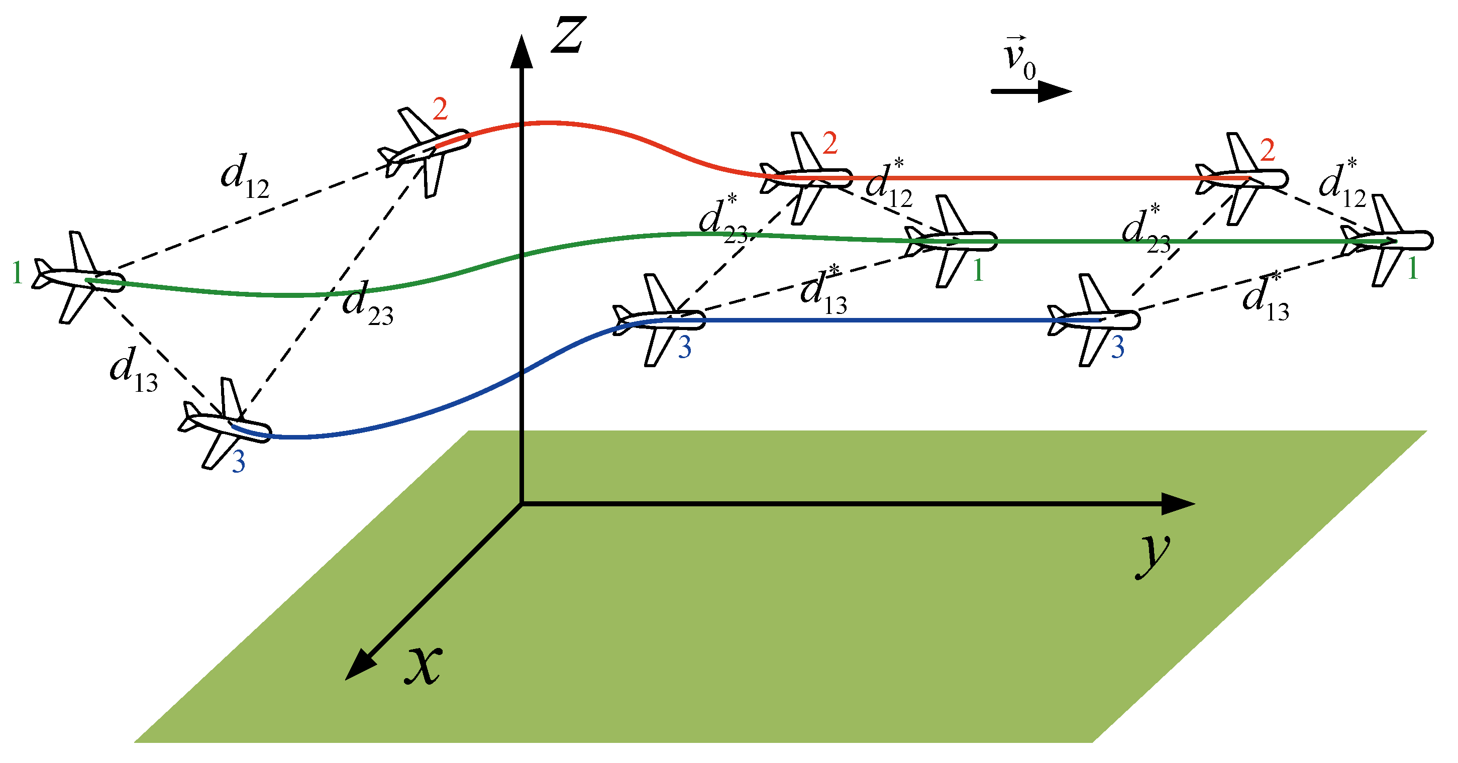
The distance-based formation usually defines the desired formation based on the distances among the UAVs. When the distance between the UAVs reaches the desired distance, the formation goal will be considered to be achieved. However, fixed-wing UAVs cannot stay still after reaching the desired distance and usually have to keep flying at a uniform velocity. Therefore, different from the distance-based formation control in reference [31], the desired formation requires not only that the desired distance between the UAVs be maintained, but also that the UAVs keep moving at a preset uniform velocity.

Therefore, the desired formation control objective can be described as follows:

$$\begin{array}{c}∥p_i\left(t\right)-p_j\left(t\right)∥\to d_{ij}^{\ast }\mathrm{as}t\to \infty ,\forall (i,j)\in \mathcal{E},\hfill \\ {\dot{p}}_i\left(t\right)-{\overrightarrow{v}}_0\to 0\mathrm{as}t\to \infty ,i=1,\dots ,N,\hfill \end{array}$$

(3)

where ${\overrightarrow{v}}_0\in {\mathbb{R}}^2$ is a constant vector.

Figure 1 illustrates the process of achieving the desired formation consisting of three fixed-wing UAVs. It can be observed that the three UAVs maintain the desired distance from their neighbors while moving at the same velocity ${\overrightarrow{v}}_0$.

2.3. Problem Statement

Two assumptions are posed before the problem statement.

Assumption 1.

The velocity constraints of all UAVs have a common range and the uniform velocity ${\overrightarrow{v}}_0$ lies within this velocity range, i.e., $\exists v_{min},v_{max},w_{max}^r,w_{max}^l\in {\mathbb{R}}^{+}$, for $\forall i\in \{0,1,...,N\}$ it holds that

$$\begin{array}{c}0<v_{i,min}\le v_{min}<\parallel {\overrightarrow{v}}_0\parallel <v_{max}\le v_{i,max},\hfill \\ -w_{i,max}^l\le -w_{max}^l<0<w_{max}^r\le w_{i,max}^r.\hfill \end{array}$$

(4)

Assumption 2.

The distances between all UAVs are bounded, and they are all less than a known constant $d_M$, i.e.,

$$d_{ij}\le d_M,\forall (i,j)\in \mathcal{E}.$$

(5)

Thus, the formation problem is described as follows.

Problem 1.

Under Assumptions 1 and 2, the control inputs $v_i$ and $w_i$ are designed so that each UAV reaches the desired distance from its neighbors while the entire formation maneuvers at a consistent velocity, i.e., Equation (3) holds while the velocity constraint of Equation (2) is satisfied.

Remark 4.

It is obvious that Assumption 1 is a prerequisite for a formation mission to be achievable. Only if assumption 1 is satisfied, it is possible for all UAVs to be in formation at a uniform velocity.

Remark 5.

Assumption 2 is reasonable since the communication range of UAVs in reality is usually limited, and once the distance between UAVs is farther than their communication range, their interaction topology will be broken and the formation will not be implemented.

3. Controller Design

In this section, the concept of distance-based potential function is first proposed, then the designed potential function is used to design the low-gain-based controller so that the velocity constraints can be satisfied. Finally, the stability analysis of the proposed controller is presented.

3.1. Distance-Based Potential Function

Let $e_{ij}=d_{ij}-d_{ij}^{\ast }$. Then, the vector $e=[...,e_{ij},...]\in {\mathbb{R}}^m$ consists of all $e_{ij}$ where $(i,j)\in \mathcal{E}$.

Definition 1.

For each UAV i, define a distance-based potential function $F_i:{\mathbb{R}}^{2\left|{\mathcal{N}}_i\right|+1}\to \left[0,\infty \right)$ as follows:

$$F_i(p_i,\cdots ,p_j,\cdots )\stackrel{\Delta }{=}\gamma \sum _{j\in {\mathcal{N}}_i}G\left(∥p_i-p_j∥\right),$$

(6)

where $\gamma >0$ and the function G is to be determined such that $F_i$ satisfies the following assumption:

Assumption 3.

The funtion $F_i$ satisfies the following conditions:

• $F_i\ge 0$ always holds, where $F_i=0$ if and only if $∥p_i-p_j∥=d_{ij}^{\ast }$ for all $j\in {\mathcal{N}}_i$;
• For the function $g\left(x\right)\stackrel{\Delta }{=}\frac{\dot{G}\left(x\right)}{x}$, if $∥x∥\le x_M$, it holds that $∥g\left(x\right)∥\le g_M$, where $\dot{G}\left(x\right)$ denotes differentiation of the function G;
• Denote

  $$f_i\stackrel{\Delta }{=}-{\nabla }_{p_i}{F}_i=-\gamma \sum _{j\in {\mathcal{N}}_i}g\left(∥p_{ij}∥\right)p_{ij},$$

  (7)

  and there exists $r_0$ such that $f_i=0\iff F_i=0$ in $\{p:F_i\left(p\right)\le r_0\}$.

In this paper, the function $G(·)$ is designed as

$$G\left(∥p_{ij}∥\right)=\frac{1}{2}\left[\left({∥p_{ij}∥}^2+\frac{d_{ij}^{\ast 4}}{{∥p_{ij}∥}^2}\right)-d_{ij}^{\ast 2}\right].$$

(8)

Correspondingly, the function $g(·)$ is

$$g\left(∥p_{ij}∥\right)=1-\frac{d_{ij}^{\ast 4}}{{∥p_{ij}∥}^4}.$$

(9)

Remark 6.

The second term of Assumption 3 implicitly implies that the function G is differentiable. Further, the properties of the function $F_i$ are related to the ones of the function G, which means that the function G needs to be suitably selected. In fact, the function G can take many forms which were summarized in reference [15]. Furthermore, similar to Assumption 1 of reference [31], Assumption 3 is satisfied by most of the cooperative control laws including the distance-based formation control law. In addition, $r_0$ indicates the size of the attraction domain. In other words, it determines whether the system is globally or locally stable.

Remark 7.

The distance-based potential function is a cornerstone of the controller proposed in this paper. On the one hand, the distance-based potential function can be used as the Lyapunov function candidate for proving the stability of the closed-loop system, as the Lyapunov functions are usually difficult to find for nonlinear systems. On the other hand, for the multi-agent formation control problem, distance-based potential function is more visual and intuitive, which makes it easier to understand the action of the controller. In fact, it is a popular approach to design a controller based on the constructed potential function [13,14,15]. In addition, it has been pointed out by reference [15] that the attractive property of ensuring collision avoidance for the formation system can be obtained by choosing a suitable potential function.

3.2. Low-Gain-Based Controller

On the basis of the distance-based potential function $F_i$, the controller for UAV i without velocity constraints is designed as

$$\left[\begin{array}{c}{v}_i\\ w_i\end{array}\right]=\left[\begin{array}{cc}cos{\theta }_i& sin{\theta }_i\\ -sin{\theta }_i& cos{\theta }_i\end{array}\right](f_i\left(\gamma \right)+{\overrightarrow{v}}_0),$$

(10)

where $f_i\left(\gamma \right)$ is defined in Equation (7) and indicates that $f_i$ is related to the low gain coefficient $\gamma$.

For the convenience of notation, let

$$h_i={\left[\begin{array}{cc}cos{\theta }_i& sin{\theta }_i\end{array}\right]}^T, h_i^{\perp }={\left[\begin{array}{cc}-sin{\theta }_i& cos{\theta }_i\end{array}\right]}^T, h_0={\left[\begin{array}{cc}cos{\theta }_0& sin{\theta }_0\end{array}\right]}^T.$$

(11)

Thus, Equation (10) can be rewritten as

$$\begin{array}{c}{v}_i=h_i^T(f_i\left(\gamma \right)+{\overrightarrow{v}}_0),\\ w_i=h{{}_i^{\perp }}^T(f_i\left(\gamma \right)+{\overrightarrow{v}}_0).\end{array}$$

(12)

Remark 8.

$h_i$ and $h_i^{\perp }$ are widely used in reference [31,39,40], where $h_i$ is the unit vector in the heading direction of the UAV i and $h_i^{\perp }$ is the unit vector pointing to the vertical heading direction to the right. A graphical explanation for $h_i$ and $h_i^{\perp }$ is shown in Figure 2.

Then, based on Equation (12), the low-gain-based controller with velocity constraints is designed as

$$\begin{array}{c}{v}_i=sa{t}_{v_i}(h_i^T(f_i\left(\gamma \right)+{\overrightarrow{v}}_0)),\hfill \\ w_i=sa{t}_{w_i}\left(sa{t}_{w_{1i}}({(h_i^{\perp })}^T{f}_i\left(\gamma \right))+{(h_i^{\perp })}^T{\overrightarrow{v}}_0\right),\hfill \end{array}$$

(13)

where

$$\begin{array}{c}sa{t}_{v_i}\left(x\right)=\left\{\begin{array}{cc}{v}_{i,min},\hfill & x\in (-\infty ,v_{i,min})\hfill \\ x,\hfill & x\in [v_{i,min},v_{i,max}]\hfill \\ v_{i,max},\hfill & x\in (v_{i,max},+\infty )\hfill \end{array}\right.,\hfill \\ sa{t}_{w_i}\left(x\right)=\left\{\begin{array}{cc}-w_{i,max}^l,\hfill & x\in (-\infty ,-w_{i,max}^l)\hfill \\ x,\hfill & x\in [-w_{i,max}^l,w_{i,max}^r]\hfill \\ w_{i,max}^r,\hfill & x\in (w_{i,max}^r,+\infty )\hfill \end{array}\right.,\hfill \\ sa{t}_{w_{1i}}\left(x\right)=\left\{\begin{array}{cc}-w_{i,1max}^l,\hfill & x\in (-\infty ,-w_{i,1max}^l)\hfill \\ x,\hfill & x\in [-w_{i,1max}^l,w_{i,1max}^r]\hfill \\ w_{i,1max}^r,\hfill & x\in (w_{i,1max}^r,+\infty )\hfill \end{array}\right.,\hfill \end{array}$$

(14)

and the function $f_i\left(\gamma \right)$ is defined in Equation (7) while $h_i$ and $h_i^{\perp }$ are defined in Equation (11). The variables $w_{i,1max}^l$ and $w_{i,1max}^r$ are the controller parameters satisfying

$$-w_{i,max}^l\le -w_{i,1max}^l<0<w_{i,1max}^r\le w_{i,max}^r.$$

(15)

Remark 9.

On the basis of Equation (12), Equation (13) is designed to incorporate the saturation function to accommodate the input constraints. Furthermore, in the later analysis, Equation (13) will degenerate to Equation (12) when the gain γ is small enough, which is why the controller is called “low-gain-based”.

3.3. Stability Analysis

In this part, the stability of the system with the designed controller will be analyzed.

Theorem 1.

Consider a formation of N fixed-wing UAVs with unicycle dynamics (1) and input constraints (2). Suppose that Assumption 3 holds. Then, Problem 1 can be tackled with the contol inputs given by Equation (13). That is, for all init angle ${\theta }_{i0}\in (-\pi +{\theta }_0+arcsin\frac{w_{i,1max}^r}{\parallel {\overrightarrow{v}}_0\parallel },\pi +{\theta }_0-arcsin\frac{w_{i,1max}^l}{\parallel {\overrightarrow{v}}_0\parallel })$, there exists a constant ${\gamma }^{\ast }>0$ such that, for each given $\gamma \in \left(0,{\gamma }^{\ast }\right]$, the following equalities hold

$$\begin{array}{c}∥p_i\left(t\right)-p_j\left(t\right)∥\to d_{ij}^{\ast }\mathit{as}t\to \infty ,\forall (i,j)\in \mathcal{E},\hfill \\ {\dot{p}}_i\left(t\right)-{\overrightarrow{v}}_0\to 0\mathit{as}t\to \infty ,i=1,\dots ,N,\hfill \end{array}$$

(16)

where both the linear and the angular velocity constraints are satisfied.

Proof. 

The proof can be divided into three parts.

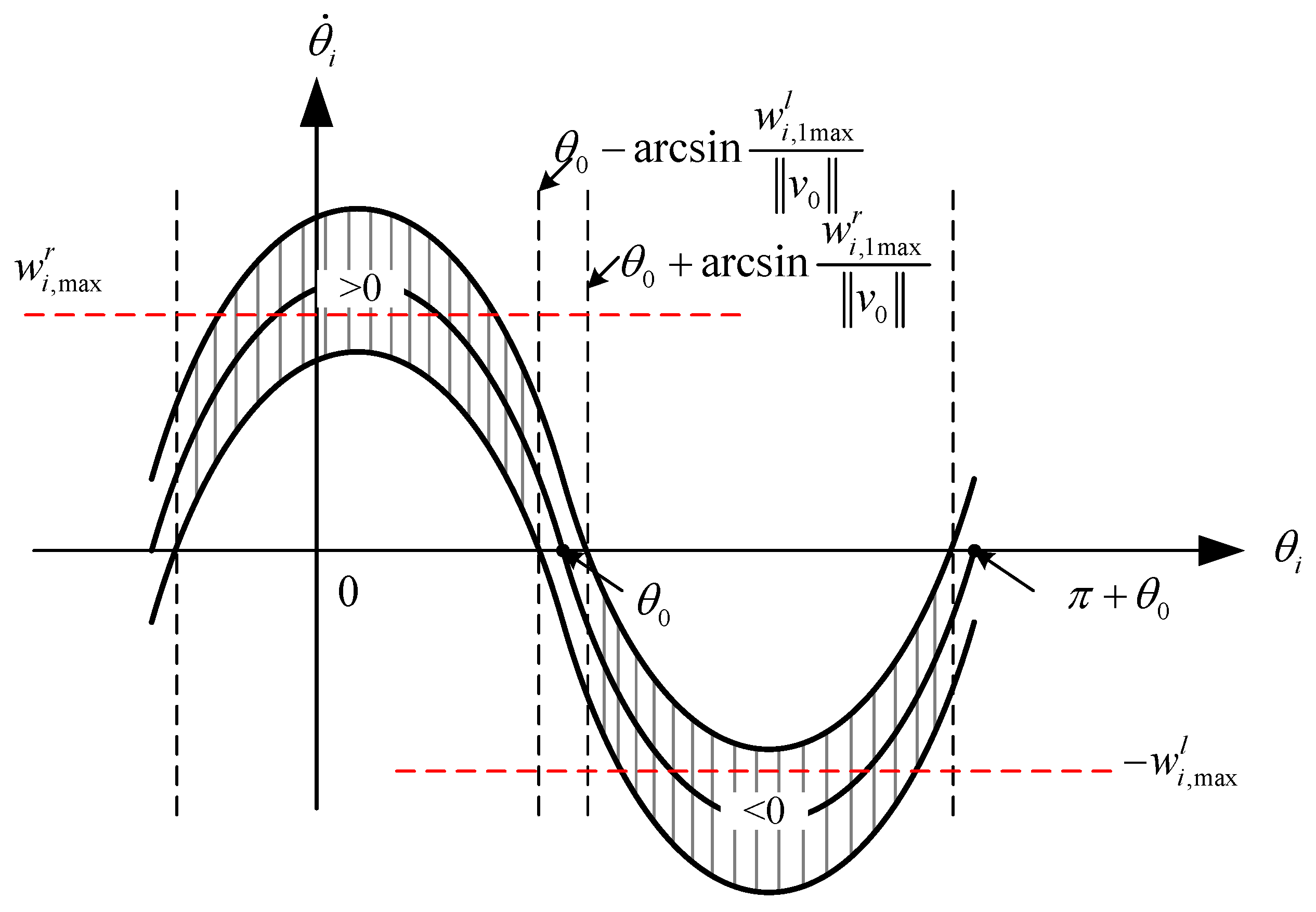
Firstly, it will be proved that the angle of each UAV under the angular velocity controller in Equation (13) will converge to a certain region. Consider the derivative of the heading angle of the UAV i

$$\begin{array}{cc}\hfill {\dot{\theta }}_i=w_i& =sa{t}_{w_i}\left(sa{t}_{w_{1i}}({(h_i^{\perp })}^T{f}_i)+{\left(h_i^{\perp }\right)}^T{\overrightarrow{v}}_0\right)\hfill \\ & =sa{t}_{w_i}\left(sa{t}_{w_{1i}}({(h_i^{\perp })}^T{f}_i)-\parallel {\overrightarrow{v}}_0\parallel sin({\theta }_i-{\theta }_0)\right)\hfill \end{array}.$$

(17)

Let $w_{i\delta }=sa{t}_{w_{1i}}({(h_i^{\perp })}^T{f}_i)\in [-w_{i,1max}^l,w_{i,1max}^r]$, then

$$\begin{array}{c}\hfill {\dot{\theta }}_i=w_i=sa{t}_{w_i}(-\parallel {\overrightarrow{v}}_0\parallel sin({\theta }_i-{\theta }_0)+w_{i\delta })\end{array}.$$

(18)

The right-hand side of Equation (18) is regarded as a function of angle ${\theta }_i$ and its graphical explanation is shown in Figure 3.

Without loss of generality, consider ${\theta }_i\in [-\pi +{\theta }_0,\pi +{\theta }_0]$. Then it holds that

$${\dot{\theta }}_i=\left\{\begin{array}{cc}>0,\hfill & {\theta }_i\in [-\pi +{\theta }_0+arcsin\frac{w_{i,1max}^r}{\parallel {\overrightarrow{v}}_0\parallel }, {\theta }_0-arcsin\frac{w_{i,1max}^l}{\parallel {\overrightarrow{v}}_0\parallel })\\ --,\hfill & {\theta }_i\in [{\theta }_0-arcsin\frac{w_{i,1max}^l}{\parallel {\overrightarrow{v}}_0\parallel }, {\theta }_0+arcsin\frac{w_{i,1max}^r}{\parallel {\overrightarrow{v}}_0\parallel }]\\ <0,\hfill & {\theta }_i\in ({\theta }_0+arcsin\frac{w_{i,1max}^r}{\parallel {\overrightarrow{v}}_0\parallel }, \pi +{\theta }_0-arcsin\frac{w_{i,1max}^l}{\parallel {\overrightarrow{v}}_0\parallel }]\end{array}\right.,$$

(19)

which means that $[{\theta }_0-arcsin\frac{w_{i,1max}^l}{\parallel {\overrightarrow{v}}_0\parallel }, {\theta }_0+arcsin\frac{w_{i,1max}^r}{\parallel {\overrightarrow{v}}_0\parallel }]$ is an atracting set for $(-\pi +{\theta }_0+arcsin\frac{w_{i,1max}^r}{\parallel {\overrightarrow{v}}_0\parallel }, \pi +{\theta }_0-arcsin\frac{w_{i,1max}^l}{\parallel {\overrightarrow{v}}_0\parallel })$, i.e., ${\theta }_i\to [{\theta }_0-arcsin\frac{w_{i,1max}^l}{\parallel {\overrightarrow{v}}_0\parallel }, {\theta }_0+arcsin\frac{w_{i,1max}^r}{\parallel {\overrightarrow{v}}_0\parallel }]\mathrm{as}t\to \infty$ while the symbol “$--$” denotes that the positive or negative sign is uncertain.

Then, the existence of $\gamma$ which makes the velocity of the UAVs unsaturated is discussed, when the angle ${\theta }_i$ converges to a certain region.

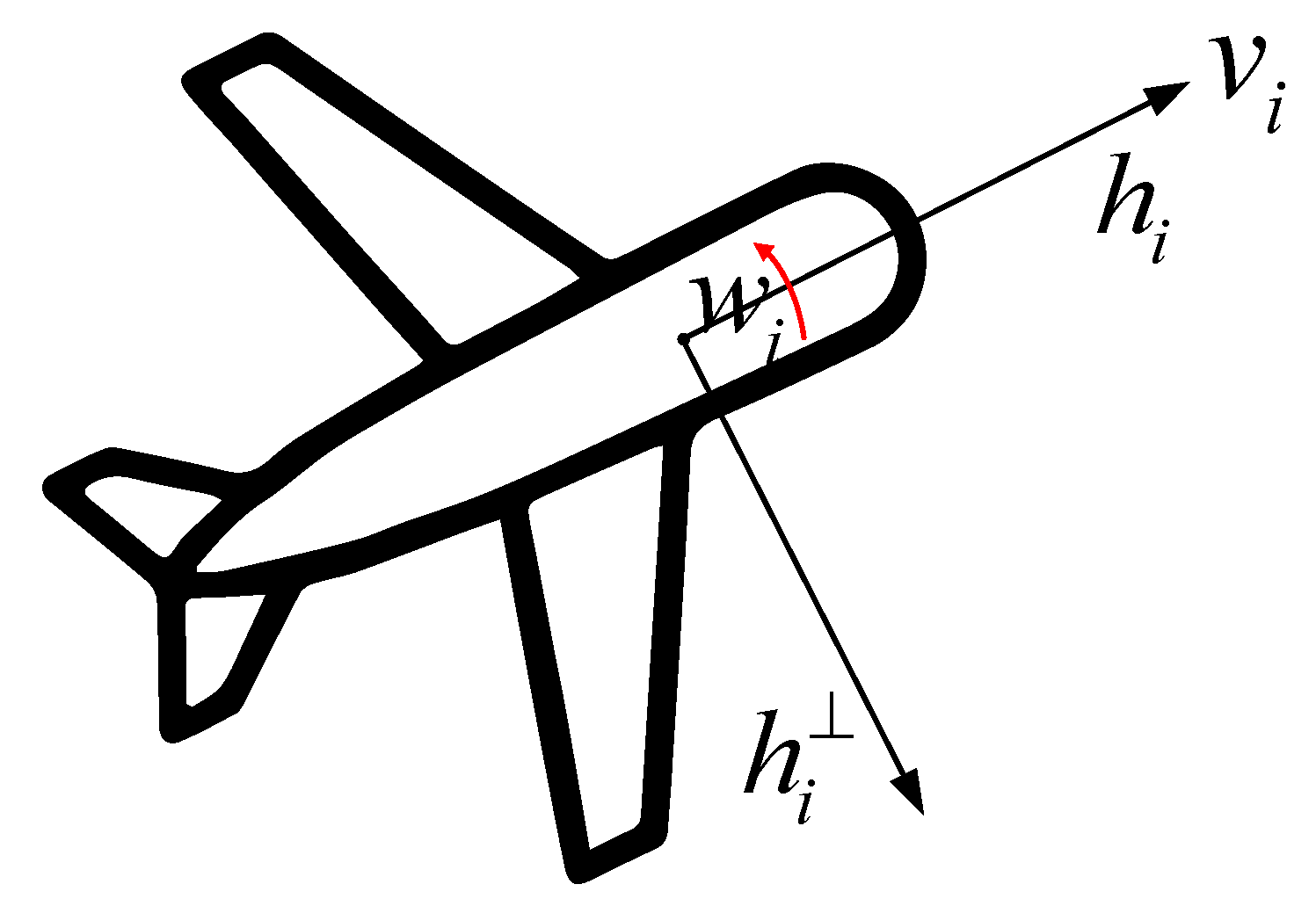
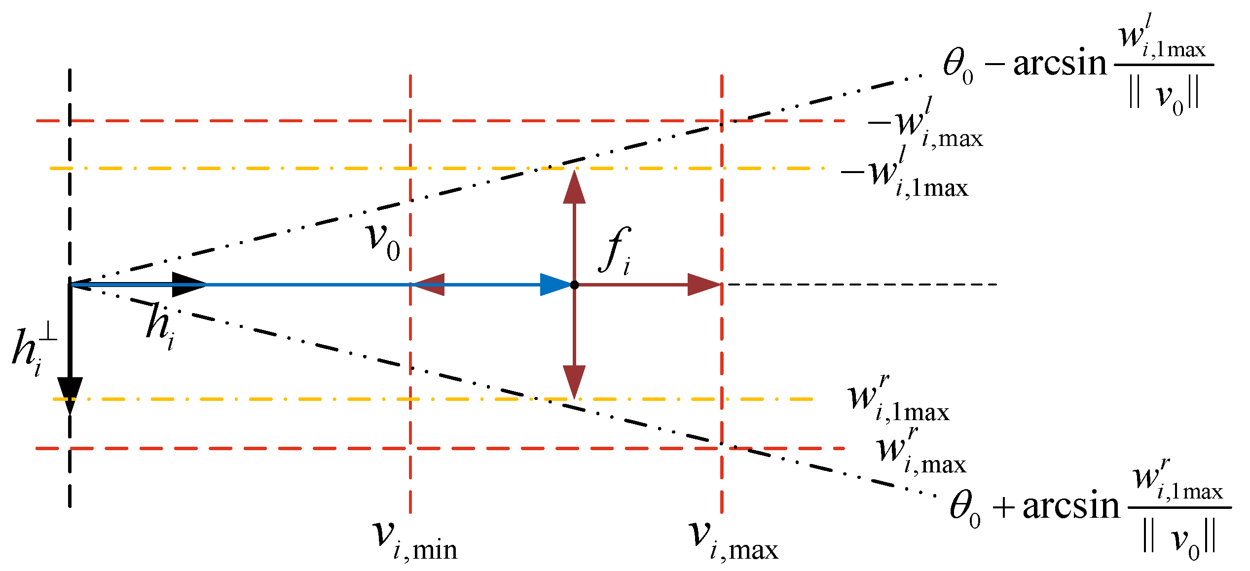
It can be observed that the linear and angular velocity controllers are the projections of vector ${\overrightarrow{v}}_0$ and vector $f_i\left(\gamma \right)$ in the direction of $h_i$ and $h_i^{\perp }$, respectively, with the saturation function added. More intuitively, a scheme of the controller is drawn as Figure 4 for the i-th UAV in the local coordinate frame.

As shown in Figure 4, the two red vertical dashed lines represent the linear velocity constraints in the forward direction, while the two red horizontal dashed lines and the two yellow horizontal dashed lines represent the maximum angular velocity constraints for $\{w_{i,max}^l,w_{i,max}^r\}$ and $\{w_{i,1max}^l,w_{i,1max}^r\}$, respectively. The blue arrow shows the vector ${\overrightarrow{v}}_0$, and the dark red arrows in four directions show the “shortest” vector $f_i\left(\gamma \right)$ that reaches the saturation condition. That is, if the “shortest” vector exists in all four directions, there exists $\gamma$ that makes all the saturation functions in Equation (13) not work due to the fact that ${lim}_{\gamma \to 0}{f}_i\left(\gamma \right)=0$.

Let the “shortest” vectors in the four directions be $f_i^{up}$, $f_i^{down}$, $f_i^{left}$, and $f_i^{right}$, respectively. Clearly as shown in Figure 4, $f_i^{right}$ reaches a minimum when the vector ${\overrightarrow{v}}_0$ and the vector $h_i$ are in the same direction, i.e.,

$${∥f_i^{right}∥}_{min}=v_{i,max}-∥{\overrightarrow{v}}_0∥.$$

(20)

Obviously, as the angle between the vector ${\overrightarrow{v}}_0$ and the vector $h_i$ changes, the “shortest” vector $f_i$ in each of the four directions changes. Consider the two extreme cases (i.e., the angle reaches its maximum) as shown in Figure 5a,b below:

From Figure 5a, the length of $f_i^{up}$ and $f_i^{left}$ in this case reaches the minimum, respectively. Further, the minimum can be obtained by the following equations, respectively:

$$\begin{array}{c}{∥f_i^{up}∥}_{min}=w_{i,max}^l-w_{i,1max}^l,\hfill \\ {∥f_i^{left}∥}_{1min}=∥{\overrightarrow{v}}_0∥cos(arcsin\frac{w_{i,1max}^l}{∥{\overrightarrow{v}}_0∥})-v_{i,min}.\hfill \end{array}$$

(21)

Furthermore, from Figure 5b, the length of $f_i^{down}$ and $f_i^{left}$ in this case reaches the minimum, respectively. Further, the minimum can be obtained by the following equations, respectively:

$$\begin{array}{c}{∥f_i^{down}∥}_{min}=w_{i,max}^r-w_{i,1max}^r,\hfill \\ {∥f_i^{left}∥}_{2min}=v_{i,max}-∥{\overrightarrow{v}}_0∥cos(arcsin\frac{w_{i,1max}^r}{∥{\overrightarrow{v}}_0∥}).\hfill \end{array}$$

(22)

Now, let $M_i=min\{{∥f_i^{up}∥}_{min},{∥f_i^{down}∥}_{min},{∥f_i^{left}∥}_{min},{∥f_i^{right}∥}_{min}\}$, where ${∥f_i^{left}∥}_{min}=min\{{∥f_i^{left}∥}_{1min},{∥f_i^{left}∥}_{2min}\}$. Then $M=\min \{\cdots ,M_i,\cdots \}$. Obviously $M>0$. Furthermore, for $f_i$, since the distance between the UAVs is bounded combined with Assumption 3, it follows that ${\displaystyle \sum _{j\in {\mathcal{N}}_i}}g\left(∥p_{ij}∥\right)$ is bounded, so there exists a sufficiently small $\gamma$ such that $f_i\left(\gamma \right)<M$ always holds.

Since $f_i\left(\gamma \right)<M$ always holds, the following inequality will hold for each UAV i

$$\begin{array}{cc}\hfill v_{i,min}& <h_i^T(f_i+{\overrightarrow{v}}_0)<v_{i,max},\hfill \\ \hfill -w_{i,1max}^l& <{\left(h_i^{\perp }\right)}^T{f}_i<w_{i,1max}^r,\hfill \\ \hfill -w_{i,max}^l& <{\left(h_i^{\perp }\right)}^T{f}_i+{\left(h_i^{\perp }\right)}^T{\overrightarrow{v}}_0<w_{i,max}^r,\hfill \end{array}$$

(23)

where Equation (13) degenerates into Equation (12) which does not involve the saturation function. This means that all velocity constraints are satisfied.

Finally, consider the Lyapunov function candidate

$$V=\frac{1}{2}\sum _{i\in \mathcal{V}}{F}_i+\sum _{i\in \mathcal{V}}∥{\overrightarrow{v}}_0∥(1-cos({\theta }_i-{\theta }_0)).$$

(24)

Taking the differential of Equation (24) yields

$$\begin{array}{cc}\hfill \dot{V}& =\frac{1}{2}\sum _{i\in \mathcal{V}}\left[\gamma \sum _{j\in {\mathcal{N}}_i}g\left(∥p_{ij}∥\right)p_{ij}^T({\dot{p}}_i-{\dot{p}}_j)\right]+\sum _{i\in \mathcal{V}}∥{\overrightarrow{v}}_0∥sin({\theta }_i-{\theta }_0)w_i\hfill \\ \hfill & =\sum _{i\in \mathcal{V}}\left[\gamma \sum _{j\in {\mathcal{N}}_i}g\left(∥p_{ij}∥\right)p_{ij}^T{\dot{p}}_i\right]-\sum _{i\in \mathcal{V}}∥{\overrightarrow{v}}_0∥h{{}_i^{\perp }}^T{h}_0{w}_i\hfill \\ \hfill & =\sum _{i\in \mathcal{V}}\left[\gamma \sum _{j\in {\mathcal{N}}_i}g\left(∥p_{ij}∥\right)p_{ij}^T{\dot{p}}_i-∥{\overrightarrow{v}}_0∥h{{}_i^{\perp }}^T{h}_0{w}_i\right]\hfill \\ \hfill & =\sum _{i\in \mathcal{V}}\left[-f_i^T{\dot{p}}_i-∥{\overrightarrow{v}}_0∥h{{}_i^{\perp }}^T{h}_0{w}_i\right]\hfill \\ \hfill & =\sum _{i\in \mathcal{V}}\left[-f_i^T{h}_i{h}_i^T(f_i+{\overrightarrow{v}}_0)-∥{\overrightarrow{v}}_0∥h{{}_i^{\perp }}^T{h}_{0}h{{}_i^{\perp }}^T(f_i+{\overrightarrow{v}}_0)\right]\hfill \\ \hfill & =\sum _{i\in \mathcal{V}}\left[-f_i^T{h}_i{h}_i^T{f}_i-f_i^T{h}_i{h}_i^T{\overrightarrow{v}}_0-h{{}_i^{\perp }}^T{\overrightarrow{v}}_{0}h{{}_i^{\perp }}^T{f}_i-h{{}_i^{\perp }}^T{\overrightarrow{v}}_{0}h{{}_i^{\perp }}^T{\overrightarrow{v}}_0\right]\hfill \\ \hfill & =\sum _{i\in \mathcal{V}}\left[-f_i^T{h}_i{h}_i^T{f}_i-f_i^T{h}_i{h}_i^T{\overrightarrow{v}}_0-f_i^T{h}_i^{\perp }h{{}_i^{\perp }}^T{\overrightarrow{v}}_0-h{{}_i^{\perp }}^T{\overrightarrow{v}}_{0}h{{}_i^{\perp }}^T{\overrightarrow{v}}_0\right]\hfill \\ \hfill & =\sum _{i\in \mathcal{V}}\left[-{\left(h_i^T{f}_i\right)}^2-{(h{{}_i^{\perp }}^T{\overrightarrow{v}}_0)}^2-f_i^T{\overrightarrow{v}}_0\right]\hfill \\ \hfill & =\sum _{i\in \mathcal{V}}\left[-{\left(h_i^T{f}_i\right)}^2-{(h{{}_i^{\perp }}^T{\overrightarrow{v}}_0)}^2+\gamma \sum _{j\in {\mathcal{N}}_i}g\left(∥p_{ij}∥\right)p_{ij}^T{\overrightarrow{v}}_0+\right]\hfill \\ \hfill & =\sum _{i\in \mathcal{V}}\left[-{\left(h_i^T{f}_i\right)}^2-{(h{{}_i^{\perp }}^T{\overrightarrow{v}}_0)}^2\right]\le 0,\hfill \end{array}$$

(25)

which implies that the system is stable. The equality $\dot{V}=0$ yields that $h_i^T{f}_i=0$ and $h{{}_i^{\perp }}^T{\overrightarrow{v}}_0=0$, which further implies that ${\theta }_i={\theta }_0$ or ${\theta }_i={\theta }_0+\pi$. However, ${\theta }_i={\theta }_0+\pi$ is impossible because the first part proves that the angle ${\theta }_i$ will converge to a certain region near ${\theta }_0$. On the other hand, the former can be considered in the following two cases:

• $f_i=0$;
• $h_i^T{f}_i=0$ but $f_i\ne 0$.

For the case 1, the desired formation is obviously achieved. The case 2 is discussed below. Consider the dynamics of UAV i’s position:

$$\begin{array}{cc}\hfill {\dot{p}}_i& =h_i{v}_i\hfill \\ \hfill & =h_{i}sat\left(h_i^T{f}_i\left(\gamma \right)+h_i^T{\overrightarrow{v}}_0\right)\hfill \\ \hfill & =h_i{h}_i^T{f}_i\left(\gamma \right)+h_i{h}_i^T{\overrightarrow{v}}_0\hfill \\ \hfill & =h_i{h}_i^T{f}_i\left(\gamma \right)+{\overrightarrow{v}}_0-h_i^{\perp }{h}_i^{\perp T}{\overrightarrow{v}}_0\hfill \\ \hfill & ={\overrightarrow{v}}_0\hfill \end{array},$$

(26)

which means that ${\theta }_i={\theta }_0$, i.e., the vector $h_i$ is invariant. Whereas considering the dynamics of the UAV i’s angle, it holds that

$$\begin{array}{cc}\hfill {\dot{\theta }}_i& =sa{t}_{w_i}\left(sa{t}_{w_{1i}}\left({\left(h_i^{\perp }\right)}^T{f}_i\left(\gamma \right)\right)+{\left(h_i^{\perp }\right)}^T{\overrightarrow{v}}_0\right)\hfill \\ \hfill & ={\left(h_i^{\perp }\right)}^T{f}_i\left(\gamma \right)+{\left(h_i^{\perp }\right)}^T{\overrightarrow{v}}_0\hfill \\ \hfill & ={\left(h_i^{\perp }\right)}^T{f}_i\left(\gamma \right)\hfill \\ \hfill & \ne 0\hfill \end{array},$$

(27)

which means that ${\theta }_i$ is always changing, so the contradiction arises and the case 2 is not valid.

With the discussion mentioned above, the system will converge to the desired formation, i.e., Equation (3) holds and the proof is complete. □

Remark 10.

The effect of low gain γ is to disable all saturation in the controller given by Equation (13). In practice, it works well to protect the fixed-wing UAV from being saturated all the time. Note that all saturation functions will not work after the angle ${\theta }_i$ converges to a certain region.

Remark 11.

Although Theorem 1 requires the initial angle of all UAVs to be within a certain region, in practice the angle is usually unstable outside of that range, and it has a tendency to enter a certain region. Therefore practically the initial angle can be arbitrary, as can be verified in the experimental results in the following part.

4. Simulations

In this section, the effectiveness of the proposed low-gain-based controller is verified in numerical and semi-physical simulations, while the corresponding simulation results are analyzed as well.

4.1. Simulation Setup

In the simulation, a formation of five fixed-wing UAVs is considered. Furthermore, the desired formation shape is a regular pentagon whose underlying graph as shown in Figure 6a where $d_{12}^{\ast }=d_{23}^{\ast }=d_{34}^{\ast }=d_{45}^{\ast }=d_{15}^{\ast }=2r_{d}sin(\pi /5)$ and $d_{25}^{\ast }=d_{35}^{\ast }=2r_{d}sin(2\pi /5)$. Additionally, the velocity constraints for each UAV i are given as follows:

$$\begin{array}{c}{v}_{i,max}=16(\mathrm{m}/\mathrm{s}),\hfill \\ v_{i,min}=10(\mathrm{m}/\mathrm{s}),\hfill \\ w_{i,max}^l=\pi /3(\mathrm{rad}/\mathrm{s}),\hfill \\ w_{i,max}^r=\pi /3(\mathrm{rad}/\mathrm{s}).\hfill \end{array}$$

(28)

Meanwhile, the direction of the uniform velocity ${\overrightarrow{v}}_0$ is shown by the arrows in Figure 6b with constant magnitude 13 m/s. In Figure 6b, the total time is divided equally into five periods, $(t_0,t_1)$, $(t_1,t_2)$, $(t_2,t_3)$, $(t_3,t_4)$ and $(t_4,t_5)$, and the desired uniform velocity ${\overrightarrow{v}}_0$ during these five periods are ${\overrightarrow{v}}_0^{\left(0\right)}$, ${\overrightarrow{v}}_0^{\left(1\right)}$, ${\overrightarrow{v}}_0^{\left(2\right)}$, ${\overrightarrow{v}}_0^{\left(3\right)}$, and ${\overrightarrow{v}}_0^{\left(4\right)}$, respectively.

Next, for each UAV i, choose the following potential function:

$$F_i=\gamma \sum _{j\in {\mathcal{N}}_i}\frac{1}{2}\left[\left({∥p_{ij}∥}^2+\frac{d_{ij}^{\ast 4}}{{∥p_{ij}∥}^2}\right)-d_{ij}^{\ast 2}\right].$$

(29)

Then

$$f_i=-{\nabla }_{p_i}{F}_i=-\gamma \sum _{j\in {\mathcal{N}}_i}\left(1-\frac{d_{ij}^{\ast 4}}{{∥p_{ij}∥}^4}\right)p_{ij}.$$

(30)

Let $w_{i,1max}^l=w_{i,1max}^r=\pi /4$ for each UAV i. It is then easy to obtain ${∥f_i^{up}∥}_{min}=0.2618$, ${∥f_i^{down}∥}_{min}=0.2618$, ${∥f_i^{left}∥}_{min}=1.9807$, ${∥f_i^{right}∥}_{min}=4$. Furthermore, note that

$$\sum _{j\in {\mathcal{N}}_i}\left(1-\frac{d_{ij}^{\ast 4}}{{∥p_{ij}∥}^4}\right)\le 4\left(1-\frac{d_{ij}^{\ast 4}}{d_M^4}\right)<4.$$

(31)

Assuming that $d_M=10$, then $\gamma$ is set as $0.0064$.

4.2. Numerical Simulation

In the numerical simulation, the initial positions of the five UAVs are ${[20,8]}^T$, ${[8,8]}^T$, ${[4,0]}^T$, ${[14,-10]}^T$, ${[24,0]}^T\left(m\right)$, and heading angles are $0\left(rad\right)$, respectively. The parameter $r_d$ is set to be 10.

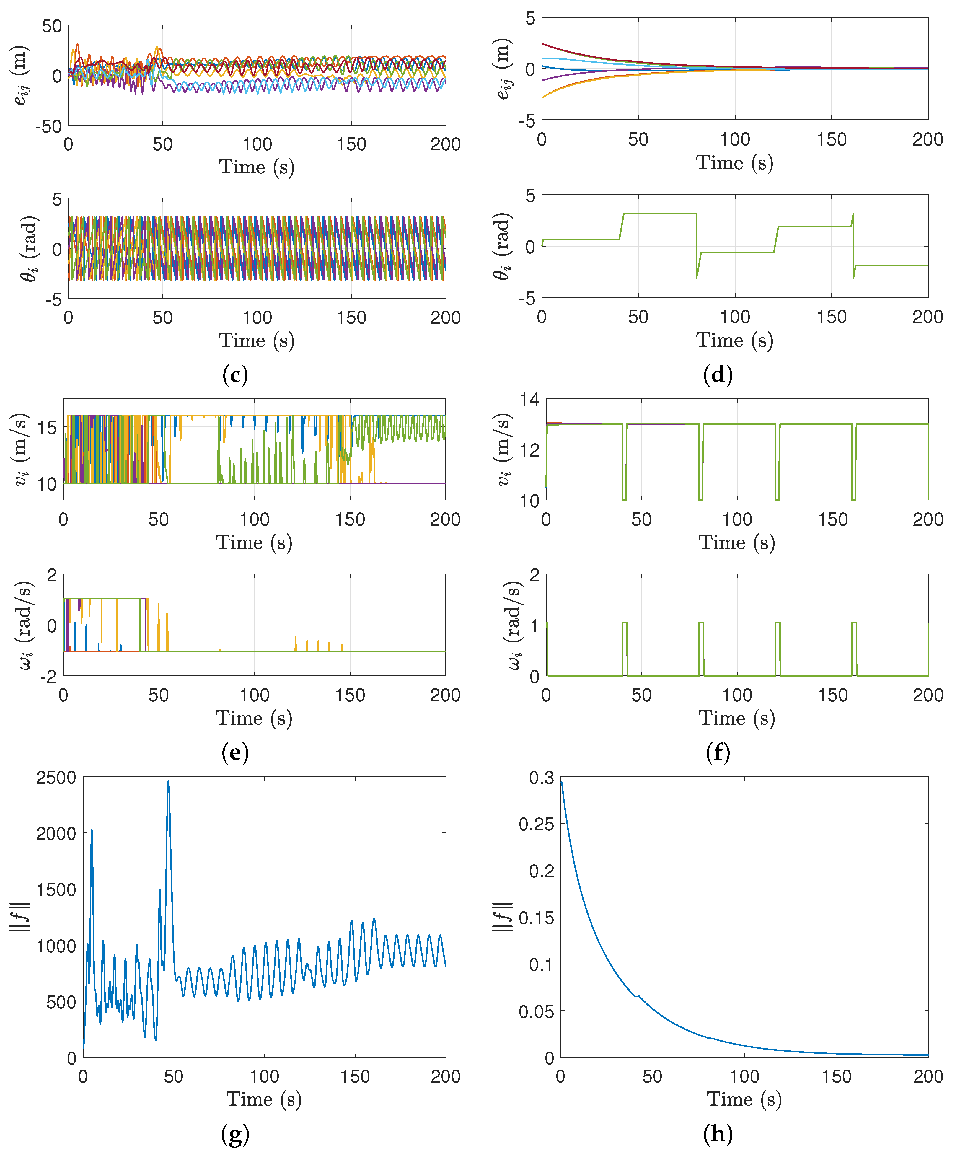
To better illustrate the impact of the input constraints on the controller design, we simulate the control algorithm proposed in the reference [23], where the controller parameters are given in the simulation part of reference [23]. It should be noted that reference [23] does not perform stability analysis of the control algorithm in the case of the presence of input constraints. Figure 7c,d illustrate the control inputs $v_i$ and $w_i$ of the algorithm proposed in reference [23] without the velocity constraints. Although the angular velocities can satisfy the constraints after saturating all velocities, it can be observed that the linear velocities still exceed the input constraints defined in Equation (2).

Then, to verify the effectiveness of the control algorithm proposed in this paper, we simulate the method proposed in [23] and our algorithm in the same situation where the constraints (2) are enforced on the UAVs. Figure 8 illustrates the numerical simulation results of the two methods. It can be seen that although the algorithm proposed in reference [23] performs well when there exists no input constraints as shown in Figure 7, the control algorithm fails when the constraints (2) are enforced on the UAVs, as shown in Figure 8. Instead, under the control of our method, the input constraints of each UAV are satisfied while the desired distance-based formation is achieved.

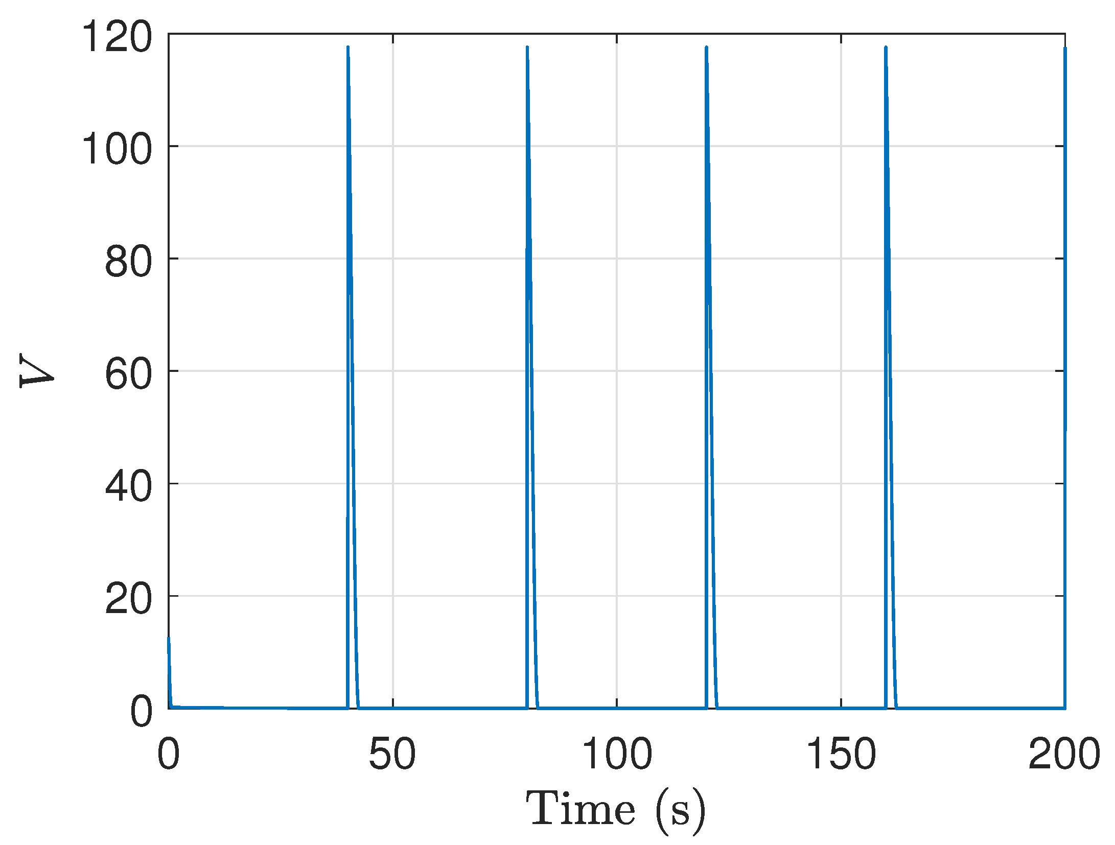
Figure 9 illustrates that the value of the Lyapunov function converges to zero. It can also be seen that there is a sharp peak in its Lyapunov function when the uniform velocity ${\overrightarrow{v}}_0$ changes. The reason for this phonomenon is that it is the uniform linear velocity rather than the uniform angular velocity that is considered in this paper.

To further illustrate that our algorithm can tackle the case of non-identical input constraints, we modify the velocity constraints of each UAV as

$$\begin{array}{cc}9\le v_1\le 15,& \left|w_1\right|\le 0.95,\\ 9.5\le v_2\le 15.5,& \left|w_2\right|\le 1,\\ 10\le v_3\le 16,& \left|w_3\right|\le 1.05,\\ 10.5\le v_4\le 16.5,& \left|w_4\right|\le 1.1,\\ 11\le v_5\le 17,& \left|w_5\right|\le 1.15,\end{array}$$

(32)

where the units of velocity and angular velocity are $m/s$ and $rad/s$, respectively.

Figure 10 and Figure 11 show the simulation results for the case of non-identical input constraints. It can be seen that the input constraints are still satisfied although the convergence time becomes longer. This is the result of a trade-off in the control algorithm.

4.3. Semi-Physical Simulation

To prove that our method can be apllied to the physical UAV system, the proposed formation controller is further validated in a semi-physical simulation system.

4.3.1. Semi-Physical Simulation System

The semi-physical simulation system consists of four main parts: onboard computer, autopilot, ground station, and switch. The relationships among them are shown in Figure 12. The functional details of each component are introduced in references [41,42].

In this simulation system, the software X-plane is used to simulate the dynamics of UAVs as well as the flight environment, which is a professional flight simulation software with powerful features, providing high precision dynamics models of UAVs and realistic 3D simulation scenarios. Meanwhile, the autopilot is used for the hardware-in-the-loop (HIL) experiment, which will further narrow the gap between the simulation and the physical reality.

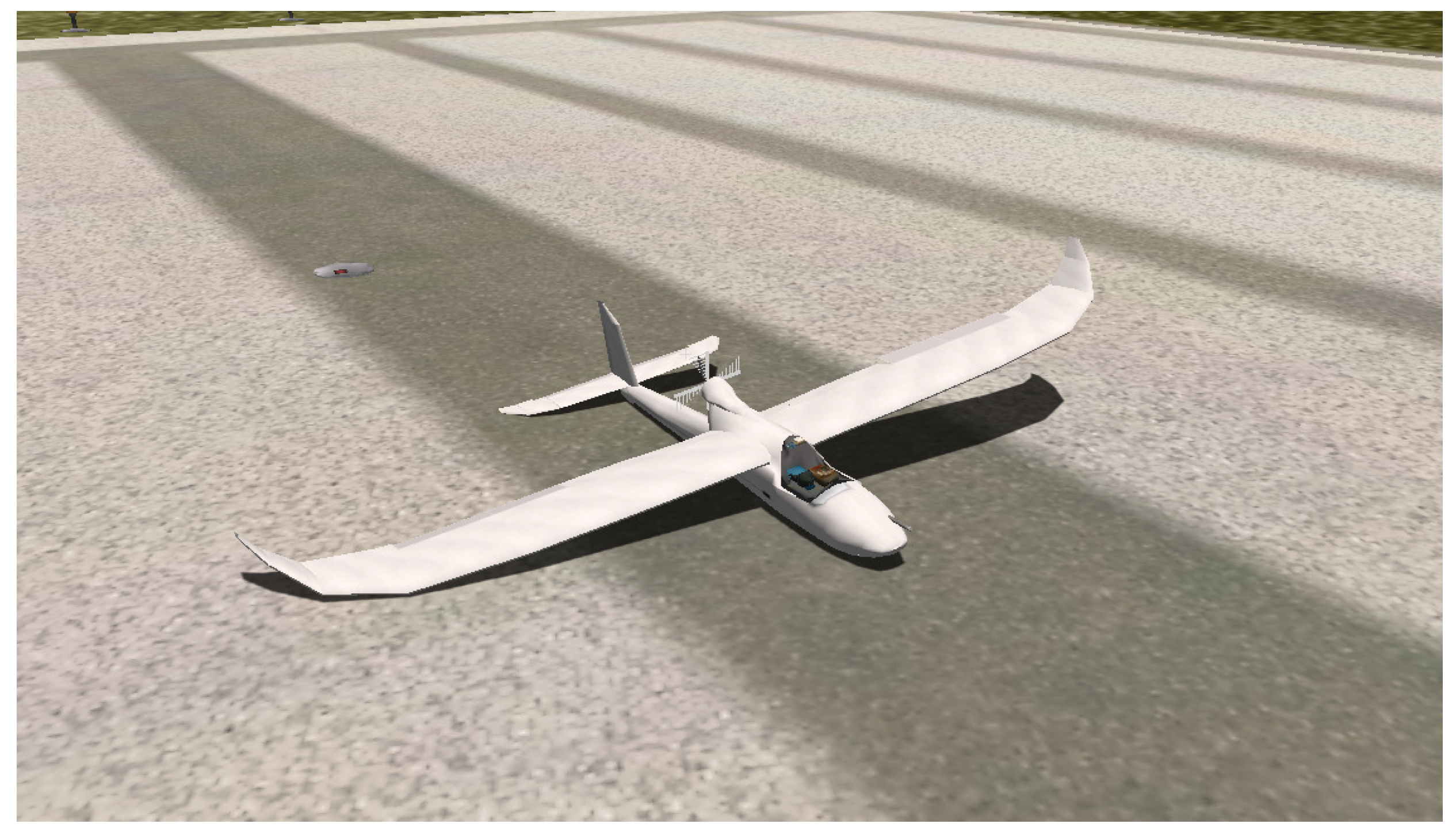
In this paper, we select the HiLStar17 as the model for the semi-physical simulation as shown in Figure 13.

4.3.2. Semi-Physical Simulation Results

In the semi-physical simulation, the parameter $r_d$ will be adjusted to 100 to accommodate the realistic formation formation flight. Then, the semi-physical simulation results are shown as follows.

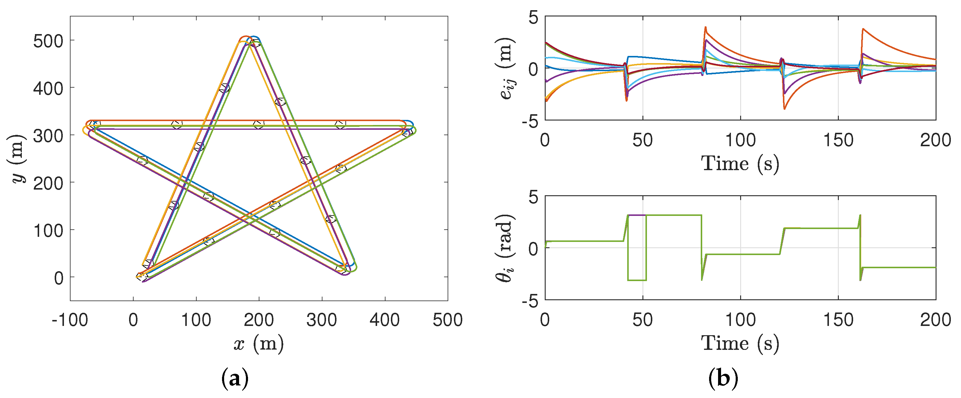
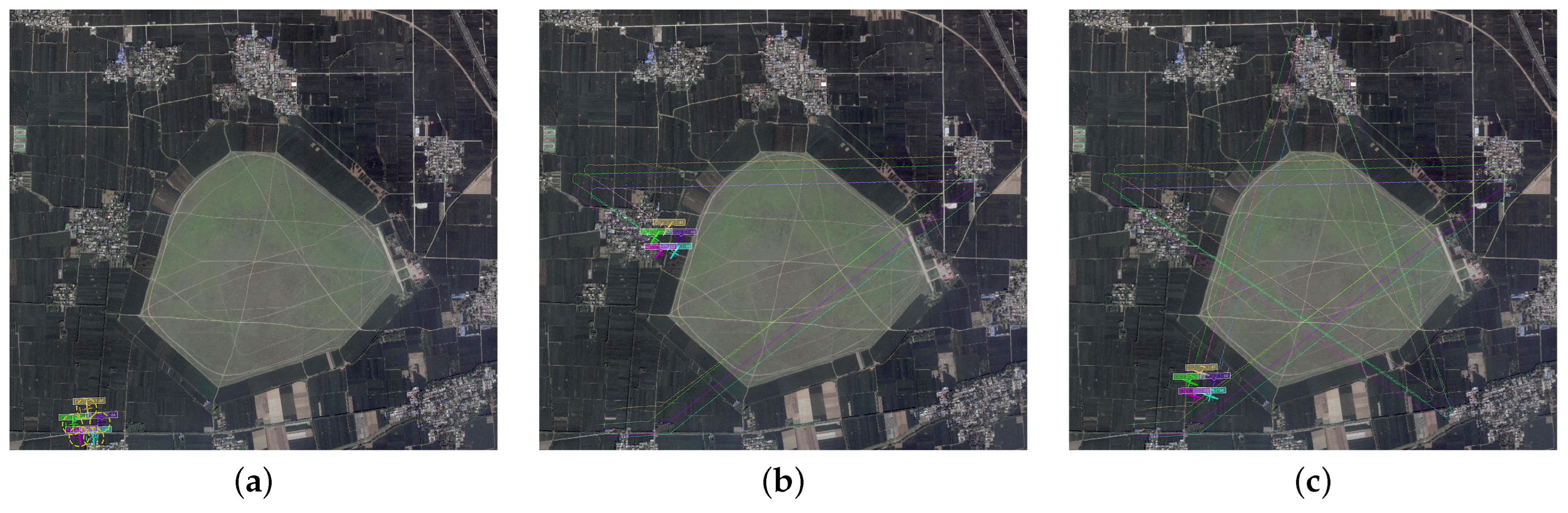
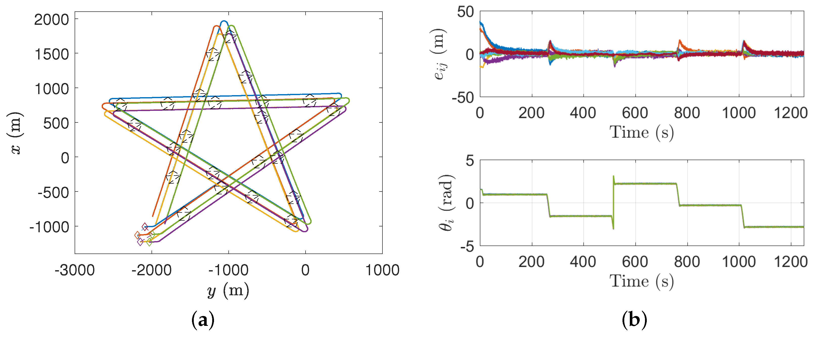
Figure 14 shows the initial position of the UAV displayed in the ground station and the evolution of the trajectory, and a more detailed trajectory is shown in Figure 15a.

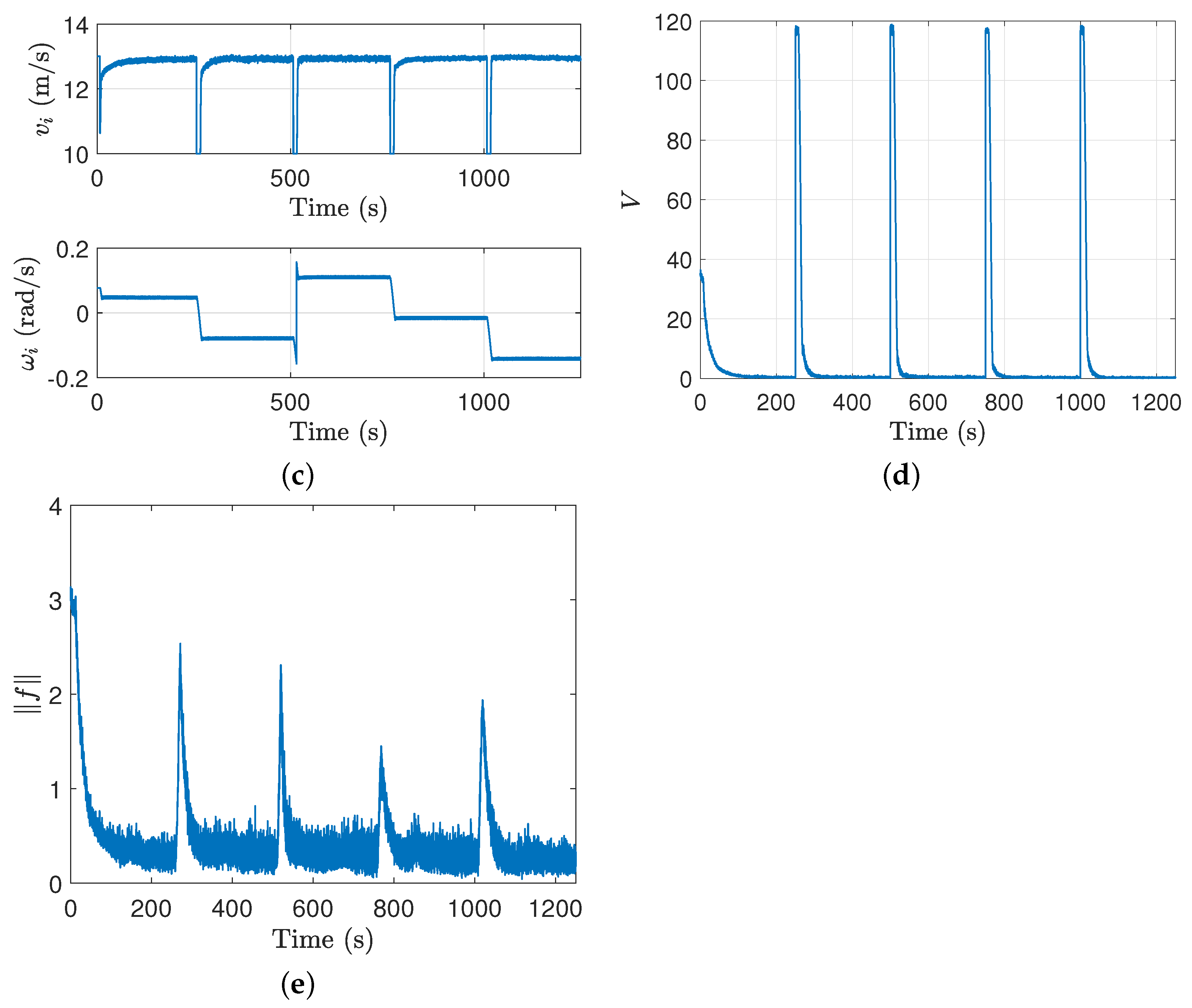
Figure 15b shows the distance error and the angle of the UAVs, which converge to the desired values. Figure 15c illustrates the variation of the control input of the UAV labeled by the number 1 during the simulation. Figure 15d then indicates that the value of Lyapunov function converges to zero. Finally Figure 15e indicates that the norm of f is gradually decreasing, which means that the control input energy of the formation is reduced.

5. Conclusions

With the idea of the low gain technique, this paper proposes a low-gain formation controller to solve the formation control problem of distance-based fixed-wing UAVs subject to the input constraints. The proposed controller is designed based on the potential function and can achieve the formation of fixed-wing UAVs while satisfying the velocity constraints. The numerical simulations and the semi-physical simulations are carried out to vefify the effectiveness of the proposed algorithm.

In the future, the formation with the uniform angular velocity will be further considered, and the obstacle avoidance algorithm will also be incorporated to consider the formation and obstacle avoidance problem as a whole.

References

- Chung, S.J.; Paranjape, A.A.; Dames, P.; Shen, S.; Kumar, V. A survey on aerial swarm robotics. IEEE Trans. Robot. 2018, 34, 837–855. [Google Scholar] [CrossRef] [Green Version]
- Chen, S.; Wu, F.; Shen, L.; Chen, J.; Ramchurn, S.D. Decentralized patrolling under constraints in dynamic environments. IEEE Trans. Cybern. 2015, 46, 3364–3376. [Google Scholar] [CrossRef] [PubMed]
- Fathian, K.; Safaoui, S.; Summers, T.H.; Gans, N.R. Robust distributed planar formation control for higher order holonomic and nonholonomic agents. IEEE Trans. Robot. 2020, 37, 185–205. [Google Scholar] [CrossRef]
- Scherer, J.; Yahyanejad, S.; Hayat, S.; Yanmaz, E.; Andre, T.; Khan, A.; Vukadinovic, V.; Bettstetter, C.; Hellwagner, H.; Rinner, B. An autonomous multi-UAV system for search and rescue. In Proceedings of the First Workshop on Micro Aerial Vehicle Networks, Systems, and Applications for Civilian Use, Florence, Italy, 18 May 2015; pp. 33–38. [Google Scholar]
- Liu, Z.; Wang, X.; Shen, L.; Zhao, S.; Cong, Y.; Li, J.; Yin, D.; Jia, S.; Xiang, X. Mission-oriented miniature fixed-wing UAV swarms: A multilayered and distributed architecture. IEEE Trans. Syst. Man Cybern. Syst. 2022, 52, 1588–1602. [Google Scholar] [CrossRef]
- Oh, K.K.; Park, M.C.; Ahn, H.S. A survey of multi-agent formation control. Automatica 2015, 53, 424–440. [Google Scholar] [CrossRef]
- Nuno, E.; Loria, A.; Hernández, T.; Maghenem, M.; Panteley, E. Distributed consensus-formation of force-controlled nonholonomic robots with time-varying delays. Automatica 2020, 120, 109114. [Google Scholar] [CrossRef]
- Maghenem, M.; Bautista, A.; Nuño, E.; Loría, A.; Panteley, E. Consensus of multi-agent systems with nonholonomic restrictions via Lyapunov’s direct method. IEEE Control Syst. Lett. 2018, 3, 344–349. [Google Scholar] [CrossRef] [Green Version]
- Babazadeh, R.; Selmic, R. Anoptimal displacement-based leader-follower formation control for multi-agent systems with energy consumption constraints. In Proceedings of the 26th Mediterranean Conference on Control and Automation, Zadar, Croatia, 19–22 June 2018; pp. 179–184. [Google Scholar]
- de Marina, H.G. Maneuvering and robustness issues in undirected displacement-consensus-based formation control. IEEE Trans. Autom. Control 2020, 66, 3370–3377. [Google Scholar] [CrossRef]
- Mehdifar, F.; Bechlioulis, C.P.; Hashemzadeh, F.; Baradarannia, M. Prescribed performance distance-based formation control of multi-agent systems. Automatica 2020, 119, 109086. [Google Scholar] [CrossRef]
- Krick, L.; Broucke, M.E.; Francis, B.A. Stabilisation of infinitesimally rigid formations of multi-robot networks. Int. J. Control 2009, 82, 423–439. [Google Scholar] [CrossRef]
- Oh, K.K.; Ahn, H.S. Formation control of mobile agents based on inter-agent distance dynamics. Automatica 2011, 47, 2306–2312. [Google Scholar] [CrossRef]
- Oh, K.K.; Ahn, H.S. Distance-based undirected formations of single-integrator and double-integrator modeled agents in n-dimensional space. Int. J. Robust. Nonlinear Control 2014, 24, 1809–1820. [Google Scholar] [CrossRef]
- Sun, Z.; Mou, S.; Anderson, B.D.; Cao, M. Exponential stability for formation control systems with generalized controllers: A unified approach. Syst. Control Lett. 2016, 93, 50–57. [Google Scholar] [CrossRef]
- Van Vu, D.; Trinh, M.H.; Nguyen, P.D.; Ahn, H.S. Distance-based formation control with bounded disturbances. IEEE Control Syst. Lett. 2020, 5, 451–456. [Google Scholar] [CrossRef]
- Mou, S.; Belabbas, M.A.; Morse, A.S.; Sun, Z.; Anderson, B.D. Undirected rigid formations are problematic. IEEE Trans. Autom. Control 2015, 61, 2821–2836. [Google Scholar] [CrossRef]
- Bae, Y.B.; Lim, Y.H.; Ahn, H.S. Distributed robust adaptive gradient controller in distance-based formation control with exogenous disturbance. IEEE Trans. Autom. Control 2020, 66, 2868–2874. [Google Scholar] [CrossRef]
- Babazadeh, R.; Selmic, R. Optimal distance-based formation producing control of multi-agent systems with energy constraints and collision avoidance. In Proceedings of the 59th IEEE Conference on Decision and Control, Nice, France, 11–13 December 2019; pp. 3847–3853. [Google Scholar]
- Wang, Y.; Cheng, L.; Hou, Z.G.; Yu, J.; Tan, M. Optimal formation of multirobot systems based on a recurrent neural network. IEEE Trans. Neural Netw. Learn. Syst. 2015, 27, 322–333. [Google Scholar] [CrossRef]
- Sun, Z.; Mou, S.; Deghat, M.; Anderson, B.D.; Morse, A.S. Finite time distance-based rigid formation stabilization and flocking. IFAC Proc. Vol. 2014, 47, 9183–9189. [Google Scholar] [CrossRef] [Green Version]
- Deghat, M.; Anderson, B.D.; Lin, Z. Combined flocking and distance-based shape control of multi-agent formations. IEEE Trans. Autom. Control 2015, 61, 1824–1837. [Google Scholar] [CrossRef] [Green Version]
- Khaledyan, M.; Liu, T.; Fernandez-Kim, V.; de Queiroz, M. Flocking and target interception control for formations of nonholonomic kinematic agents. IEEE Trans. Control Syst. Technol. 2019, 28, 1603–1610. [Google Scholar] [CrossRef] [Green Version]
- Chen, J.; Sun, D.; Yang, J.; Chen, H. Leader-follower formation control of multiple non-holonomic mobile robots incorporating a receding-horizon scheme. Int. J. Robot. Res. 2010, 29, 727–747. [Google Scholar] [CrossRef]
- Dong, W.; Farrell, J.A. Decentralized cooperative control of multiple nonholonomic dynamic systems with uncertainty. Automatica 2009, 45, 706–710. [Google Scholar] [CrossRef]
- Gazi, V.; Fidan, B.; Ordonez, R.; İlter Köksal, M. A target tracking approach for nonholonomic agents based on artificial potentials and sliding mode control. J. Dyn. Syst. Meas. Control 2012, 134, 061004. [Google Scholar] [CrossRef]
- Consolini, L.; Morbidi, F.; Prattichizzo, D.; Tosques, M. Leader–follower formation control of nonholonomic mobile robots with input constraints. Automatica 2008, 44, 1343–1349. [Google Scholar] [CrossRef]
- Yu, X.; Liu, L. Distributed formation control of nonholonomic vehicles subject to velocity constraints. IEEE Trans. Ind. Electron. 2015, 63, 1289–1298. [Google Scholar] [CrossRef]
- Meng, Z.; Zhao, Z.; Lin, Z. On global leader-following consensus of identical linear dynamic systems subject to actuator saturation. Syst. Control Lett. 2013, 62, 132–142. [Google Scholar] [CrossRef]
- Wang, X.; Yu, Y.; Li, Z. Distributed sliding mode control for leader-follower formation flight of fixed-wing unmanned aerial vehicles subject to velocity constraints. Int. J. Robust. Nonlinear Control 2021, 31, 2110–2125. [Google Scholar] [CrossRef]
- Zhao, S.; Dimarogonas, D.V.; Sun, Z.; Bauso, D. A general approach to coordination control of mobile agents with motion constraints. IEEE Trans. Autom. Control 2017, 63, 1509–1516. [Google Scholar] [CrossRef] [Green Version]
- Zheng, Z.; Yi, H. Backstepping control design for UAV formation with input saturation constraint and model uncertainty. In Proceedings of the 36th Chinese Control Conference, Dalian, China, 26–28 July 2017; pp. 6056–6060. [Google Scholar]
- Wei, J.; Li, H.; Guo, M.; Li, J.; Huang, H. Backstepping control based on constrained command filter for hypersonic flight vehicles with AOA and actuator constraints. Int. J. Aerosp. Eng. 2021, 2021, 8620873. [Google Scholar] [CrossRef]
- Zhao, M.; Peng, Y.; Wang, Y.; Zhang, D.; Luo, J.; Pu, H. Concise leader-follower formation control of underactuated unmanned surface vehicle with output error constraints. Meas. Control 2022, 44, 1081–1094. [Google Scholar] [CrossRef]
- Su, H.; Chen, M.Z.; Lam, J.; Lin, Z. Semi-global leader-following consensus of linear multi-agent systems with input saturation via low gain feedback. IEEE Trans. Circuits Syst. I Regul. Pap. 2013, 60, 1881–1889. [Google Scholar] [CrossRef] [Green Version]
- Chang, J.L. Robust low gain output feedback sliding mode control design against actuator saturation. IMA J. Math. Control Inf. 2019, 36, 1237–1253. [Google Scholar]
- Xu, J.; Lin, Z. Low gain feedback for fractional-order linear systems and semi-global stabilization in the presence of actuator saturation. Nonlinear Dyn. 2022, 107, 3485–3504. [Google Scholar] [CrossRef]
- Zhao, G.; Wang, Z.; Fu, X. Fully distributed dynamic event-triggered semiglobal consensus of multi-agent uncertain systems with input saturation via low-gain feedback. Int. J. Control Autom. Syst. 2021, 19, 1451–1460. [Google Scholar] [CrossRef]
- Li, H.; Chen, H.; Yang, S.; Wang, X. Standard formation generation and keeping of unmanned aerial vehicles through a potential functional approach. In Proceedings of the 39th Chinese Control Conference, Shenyang, China, 27–29 July 2020; pp. 4771–4776. [Google Scholar]
- Li, H.; Chen, H.; Wang, X. Affine formation tracking control of unmanned aerial vehicles. Front. Inf. Technol. Electron. Eng. 2022, 1–11. [Google Scholar] [CrossRef]
- Yan, C.; Xiang, X.; Wang, C.; Lan, Z. Flocking and collision avoidance for a dynamic squad of fixed-wing UAVs using deep reinforcement learning. In Proceedings of the 2021 IEEE/RSJ International Conference on Intelligent Robots and Systems, Prague, Czech Republic, 27 September 2021; pp. 4738–4744. [Google Scholar]
- Chen, H.; Wang, X.; Shen, L.; Yu, Y. Coordinated path following control of fixed-wing unmanned aerial vehicles in wind. ISA Trans. 2022, 122, 260–270. [Google Scholar] [CrossRef]
Figure 1.
The desired formation of three UAVs.
Figure 2.
The illustrations of and .
Figure 3.
The explanation of Equation (18).
Figure 4.
An intuitive presentation about the proposed controller with input constraints.
Figure 5.
Two extreme cases where the angle reaches its maximum. (a) An extreme case where is equal to . (b) Another extreme case where is equal to .
Figure 6.
The illustration of some simulation settings. (a) The underlying graph of five fixed-wing UAVs. (b) The setting of .
Figure 7.
Numerical simulation results of the method proposed in [23] without input constraints. (a) The illustration of trajectory of the five UAVs controlled by the method proposed in [23] without input constraints. (b) The illustration of distance errors and controlled by the method proposed in [23] without input constraints. (c) The linear velocity inputs of the five UAVs controlled by the method proposed in [23] without input constraints. (d) The angular velocity inputs of the five UAVs controlled by the method proposed in [23] without input constraints.
Figure 8.
The method in reference [23] vs. our method. (a) The illustration of trajectory of the five UAVs controlled by the method proposed in [23]. (b) The illustration of trajectory of the five UAVs controlled by our method. (c) The illustration of distance errors and controlled by the method proposed in [23]. (d) The illustration of distance errors and controlled by our method. (e) The illustration of control input and controlled by the method proposed in [23]. (f) The illustration of control input and controlled by our method. (g) The illustration of the norm of f controlled by the method proposed in [23]. (h) The illustration of the norm of f controlled by our method.
Figure 9.
The illustration of Lyapunov function controlled by our method.
Figure 10.
Numerical simulation results for the case of non-identical input constraints. (a) The illustration of trajectory of the five UAVs controlled by our method with non-identical input constraints. (b) The illustration of distance errors and controlled by our method with non-identical input constraints.
Figure 11.
Numerical simulation results for the case of non-identical input constraints. (a) The illustration of control input and controlled by our method with non-identical input constraints. (b) The illustration of Lyapunov function controlled by our method with non-identical input constraints.
Figure 12.
The components of semi-physical simulation system.
Figure 13.
The UAV model used in this paper.
Figure 14.
The evolution of the trajectory. (a) Initial positions. (b) Positions at 583 s. (c) Positions at 1248 s.
Figure 15.
Semi-physical simulation results. (a) The illustration of trajectory of the five UAVs in the semi-physical simulation. (b) The illustration of distance errors and in the semi-physical simulation. (c) The illustration of control input and in the semi-physical simulation. (d) The illustration of Lyapunov function in the semi-physical simulation. (e) The illustration of the norm of f in the semi-physical simulation.
Publisher’s Note: MDPI stays neutral with regard to jurisdictional claims in published maps and institutional affiliations. |
© 2022 by the authors. Licensee MDPI, Basel, Switzerland. This article is an open access article distributed under the terms and conditions of the Creative Commons Attribution (CC BY) license (https://creativecommons.org/licenses/by/4.0/).
Share and Cite
MDPI and ACS Style
Yan, J.; Yu, Y.; Wang, X. Distance-Based Formation Control for Fixed-Wing UAVs with Input Constraints: A Low Gain Method. Drones 2022, 6, 159. https://0-doi-org.brum.beds.ac.uk/10.3390/drones6070159
AMA Style
Yan J, Yu Y, Wang X. Distance-Based Formation Control for Fixed-Wing UAVs with Input Constraints: A Low Gain Method. Drones. 2022; 6(7):159. https://0-doi-org.brum.beds.ac.uk/10.3390/drones6070159
Chicago/Turabian StyleYan, Jiarun, Yangguang Yu, and Xiangke Wang. 2022. "Distance-Based Formation Control for Fixed-Wing UAVs with Input Constraints: A Low Gain Method" Drones 6, no. 7: 159. https://0-doi-org.brum.beds.ac.uk/10.3390/drones6070159