
LiDAR Based Detect and Avoid System for UAV Navigation in UAM Corridors

Engineering Physics Group, School of Aerospace Engineering, University of Vigo, Campus Ourense, 32004 Ourense, Spain
*
Author to whom correspondence should be addressed.
Drones 2022, 6(8), 185; https://0-doi-org.brum.beds.ac.uk/10.3390/drones6080185
Submission received: 29 June 2022
/
Revised: 20 July 2022
/
Accepted: 21 July 2022
/
Published: 22 July 2022
Abstract
:In this work, a Detect and Avoid system is presented for the autonomous navigation of Unmanned Aerial Vehicles (UAVs) in Urban Air Mobility (UAM) applications. The current implementation is designed for the operation of multirotor UAVs in UAM corridors. During the operations, unauthorized flying objects may penetrate the corridor airspace posing a risk to the aircraft. In this article, the feasibility of using a solid-state LiDAR (Light Detecting and Ranging) sensor for detecting and positioning these objects was evaluated. For that purpose, a commercial model was simulated using the specifications of the manufacturer along with empirical measurements to determine the scanning pattern of the device. With the point clouds generated by the sensor, the system detects the presence of intruders and estimates their motion to finally compute avoidance trajectories using a Second Order Cone Program (SOCP) in real time. The method was tested in different scenarios, offering robust results. Execution times were of the order of 50 milliseconds, allowing the implementation in real time on modern onboard computers.
1. Introduction
Urban Air Mobility (UAM) is a concept that aims to improve the efficiency of the urban and interurban system through the use of UAVs (Unmanned Aerial Vehicles) for the transport of people and goods. At the European level, it is important to highlight the U-Space project, coordinated by Single European Sky ATM (Air Traffic Management) Research (SESAR), and in which different public and private entities collaborate for the progressive implementation of the UAM [1]. The U-Space Blueprint [2] defines the main technological challenges for the implementation of the UAM, as well as the future objectives to be achieved. The aim is to progressively increase the automation of UAV operations, so that in the future high volumes of air traffic can be managed in complex navigation environments such as a city [3,4].
For the development of these operations, in accordance with the FAA (Federal Aviation Administration) Concept of Operations [5], new infrastructures will be necessary, the so called UAM corridors, which are aerial highways free from obstacles that connect several landmarks of a city. These air spaces would be adapted dynamically based on factors such as the weather, traffic congestion and time of day [6]. Nowadays, countries such as South Korea are already testing this concept and they intend to have several UAM corridors operational by 2025 [7].
Currently, most UAV flights are carried out in VLOS (Visual Line of Sight), that is, operations in which there is a person who maintains unaided visual contact with the aircraft to ensure the safety of operations. However, in the future, with the development of the UAM, new operations are expected, involving BVLOS (Beyond Visual Line of Sight) flights or even autonomous ones. For this purpose, according to U-Space, it is necessary to develop aircraft with a higher level of autonomy. Security and social acceptance are key factors for the definitive implementation of the UAM [8,9], and there are still multiple technological and legal challenges to overcome.
In the future, it is planned to use active surveillance protocols such as ADS-B (Automatic Dependent Surveillance Broadcast) to obtain the position of the aircraft operating in the urban environment [10]. In this way, from a ground station, air traffic can be managed to guarantee the safety of operations. However, at low altitudes, flying objects such as unauthorized UAVs or birds may penetrate the airspace of the UAM corridors, posing a risk to the aircraft. In addition, during the operations, failures in the communication protocols may occur, leaving the aircraft unattended during the flight with the associated risk [11]. Therefore, for these reasons, it is necessary for aircraft to have Detect and Avoid systems to solve these contingencies.
Detect and Avoid systems are based on the use of sensors to detect and position obstacles to subsequently establish maneuvers to guarantee the safety of the aircraft [12]. One of the main candidate technologies are solid-state LiDAR (Light Detecting And Ranging) sensors. These devices emit infrared light beams in different directions to measure the time of flight and obtain three-dimensional reconstructions of the navigation environment [13]. It is an active technology that does not depend on lighting conditions for its operation, which provides a greater robustness in night situations. In addition, by obtaining the distance measurements through the time of flight, they do not require processing to generate the 3D scene [14]. Furthermore, thanks to the development of robotics and autonomous driving [15], the cost of this technology has declined considerably, and nowadays there are light (about 500 g) and precise commercial sensors for prices below 1000 US dollars.
In this work, the feasibility of using a Livox Avia sensor for the detection of aerial obstacles was evaluated. For this purpose, the behavior of the sensor was simulated using Ray Tracing techniques [16]. Besides, experimental measurements were carried out to determine the scanning pattern and the technical specifications were considered to model the measurement errors of the device. Artificial point clouds of dynamic environments were generated to assess the capabilities of the sensor to detect moving obstacles.
With these point clouds, the geospatial information was processed to determine the position and velocity of the obstacles of the navigation environment. The trajectory and the equations of motion of the UAV were discretized to obtain a Second Order Cone Program (SOCP), with which avoidance trajectories were calculated in real time. SOCP is a particular type of Non-Linear Program (NLP) in which a linear objective function is minimized subject to linear and second order constraints [17].
Previous works have used NLPs for the development of obstacle avoidance solutions, but they obtained computation times of up to several seconds [18,19]. NLP problems, in their general case, are of the NP-Hard type, that is, the computation time increases exponentially with the number of variables. To address this problem, recent obstacle avoidance solutions based on NLPs limited the use of non-linear constraints to only equality relations, reducing the complexity of these non-convex problems and obtaining affordable computation times using quasi-Newton numerical methods [20,21]. In this work, instead of limiting the constraints to equality relations, an equivalent methodology is proposed through inequality conic constraints, converting the problem into a convex SOCP. Convergence times of SOCPs are generally lower than for NLPs in their generic form as they are convex problems. In fact, with numerical schemes based on interior-point methods and other techniques [22,23,24] computation times of the order of 0.1 s can be obtained [17].
The main advantage of SOCPs and NLPs over state-of-the-art obstacle avoidance is their ability to adapt to the characteristics of the detection system and the UAV and anticipate the motion of the obstacles no matter how far they are. Other proposals such as those based on geometric relationships [25,26], fuzzy logic [27,28] or potential fields [29,30,31] only apply corrections to the trajectory when the UAV is at a distance less than a threshold value from the obstacle. When the distance is greater, the algorithms do not act, and the UAV continues with its original trajectory. This can be a problem if the obstacles are moving at a considerable speed, since the minimum distance considered by these methods could be insufficient and the UAV would not be able to react in time. In SOCP methods this does not happen, as since the moment the detection system anticipates a risk of collision, an avoidance path is automatically calculated considering the performances of the UAV. In addition, unlike other methods such as those based on neural networks [32,33], no training is required, nor the generation of study cases for the implementation.
For these reasons, SOCPs are commonly used in guidance and control applications to calculate actions that optimize a certain objective. Previous works [34,35,36] developed SOCP path planning algorithms for UAV navigation between waypoints in a scenario with multiple fixed obstacles. The previous implementations allowed the calculation of routes in real time, with computation times of the order of 100 ms, according to the authors. Zhang et al. presented an algorithm for the calculation of landing trajectories of multirotor UAVs on mobile platforms [37]. Based on a prediction of the movement of the platform, the algorithm estimates a trajectory that minimizes the flight time and the actions necessary for landing on the platform.
Other applications in the field of trajectory calculation in aerospace engineering are the calculation of actions in atmospheric re-entry maneuvers or the guidance of Air-to-Ground Missiles [38,39,40,41]. They are also used in other applications, where computing time is critical, such as attitude control and space landing maneuvers [41,42,43,44]. These methods are very flexible and can be adapted for the modelling of multiple physical systems. In this work, considering the detection capabilities of LiDAR technology and the operational characteristics of a typical multirotor UAV, a dynamic obstacle avoidance algorithm based on SOCP was implemented, which allows the calculation of avoidance trajectories that minimize the flight time between different points in an UAM corridor.
The manuscript is organized as follows: Section 2 presents the methodology, introducing the simulation environment and the trajectory computation algorithm. In Section 3, different study cases are analyzed to assess the performance of the implementation and the computational cost. In Section 4 the final conclusions are presented as well as future works and improvements.
2. Methodology
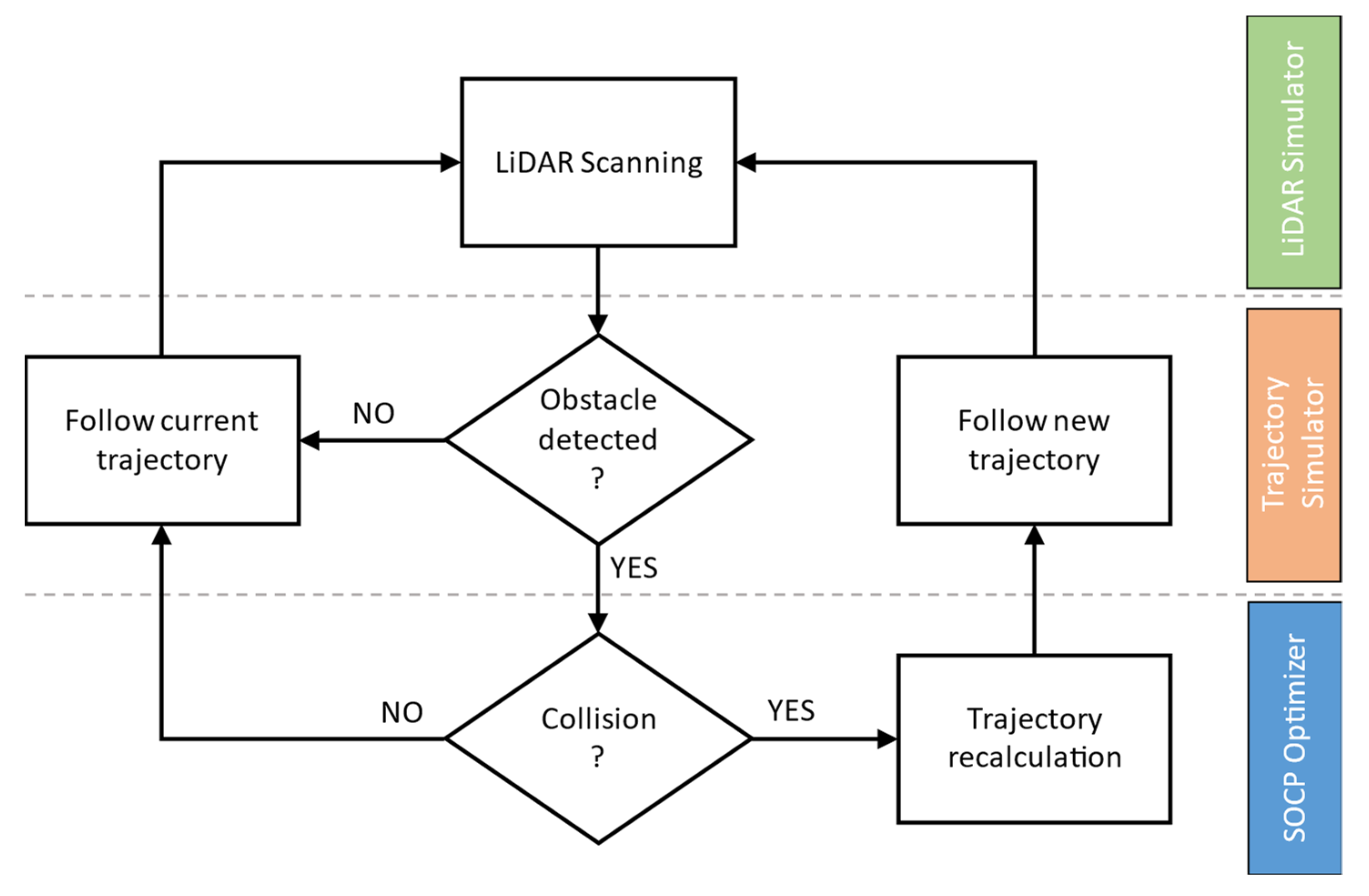
Figure 1 presents the implementation scheme of this work. For the validation of the Detect and Avoid system, three clearly differentiated blocks were developed, as it is depicted in the figure. The first one is the Trajectory Simulator, which generates the trajectories of the UAV, as well as the different obstacles in the navigation environment. During the flight, the LiDAR Simulator replicates in real time the point clouds that would be obtained when using a real onboard sensor. With this information, the Detect and Avoid system identifies the different obstacles in the environment and estimates their trajectory to check if there is a possible risk of collision. Based on this prediction, the aircraft will follow the current trajectory or activate the obstacle avoidance system based on the SOCP Optimizer to guarantee the safety of operations.
2.1. LiDAR Simulation
In this work, a Livox Avia was simulated. It is a solid-state LiDAR sensor manufactured by Livox Technology, that it is mainly oriented to robotics, mapping, and position awareness applications. Table 1 shows the sensor’s specifications, according to the manufacturer [45].
In this case, this LiDAR sensor is a time-of-flight device whose operating principle is based on sending pulses of infrared light to measure the distance in different directions. These kind of LiDAR sensors typically have one or more light beams that can be directed forming scanning patterns to obtain 3D point clouds of the sensor environment. These scanning patterns are specific of each model and may vary depending on the field of view and point rate of the sensor. Livox Avia has an elliptic petal scan pattern composed of six light beams. These rays are synchronized with the internal clock of the sensor and rotate to form the scanning pattern.
In this work, the scanning pattern of the device was determined experimentally. For this purpose, a flat wall with good reflectivity was scanned and a point cloud was sampled during an acquisition time of three seconds. With the points of the cloud, the directions of the rays were projected on a plane located one meter away from the sensor (plane X = 1). To recover possible rays that did not return to the sensor correctly, a linear interpolation was implemented to approximate these values through the measurements of contiguous rays. Figure 2 represents the scanning pattern obtained for a time of 0.08 s. As it can be appreciated, the sensor periodically phases out the petals of the pattern to progressively cover the field of view.
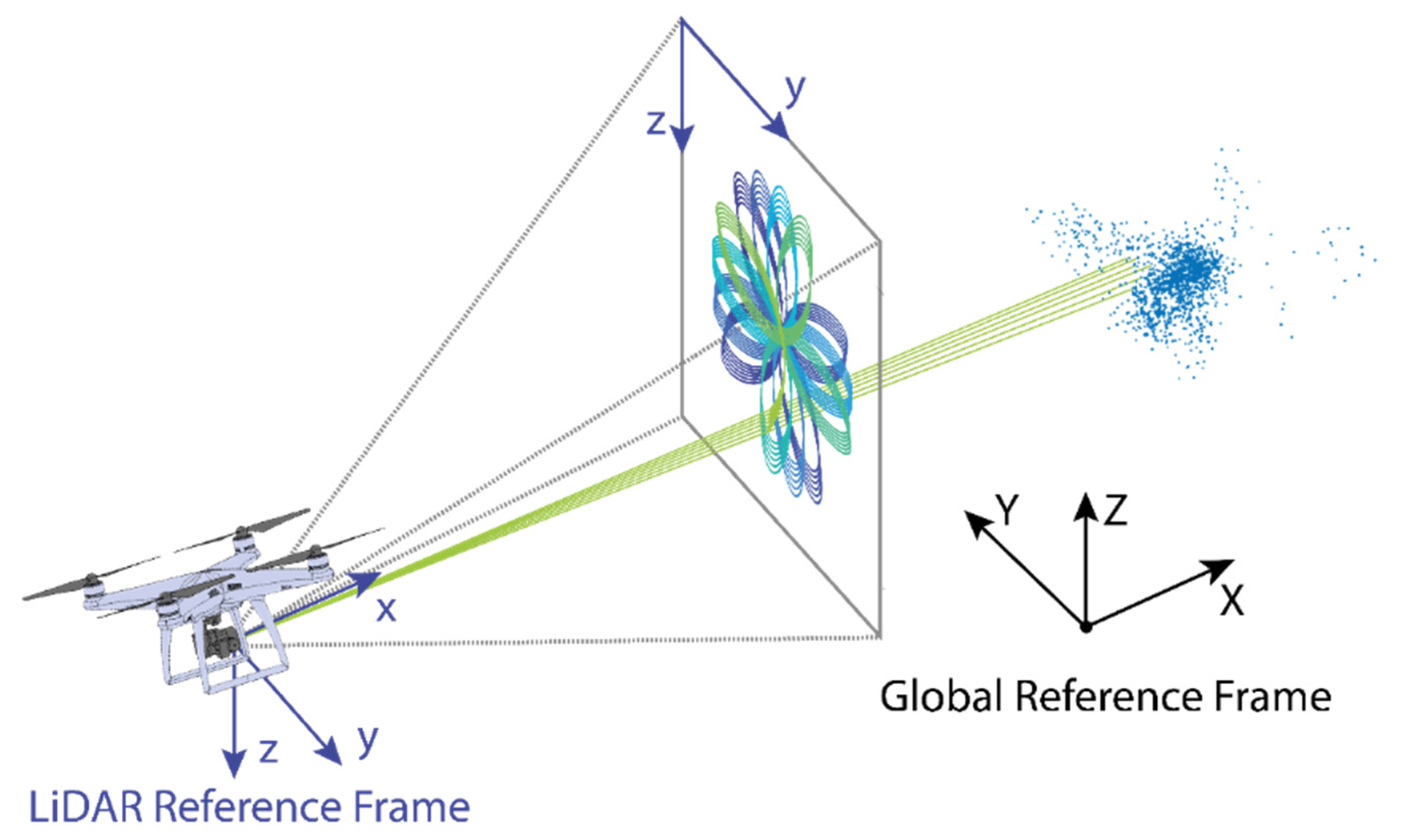
With this scanning pattern, the propagation of rays within the UAV operating scenario was simulated. Two reference frames were defined as it is depicted in Figure 3: The LiDAR reference frame, which has the origin at the center of the LiDAR sensor and whose x axis is aligned with the perpendicular axis to the device; and the Global reference frame, a Cartesian coordinate axis corresponding to the UAV’s navigation environment. The LiDAR sensor model was integrated into the trajectory simulator considering the relative pose of the UAV. For this, the translations and rotation matrices corresponding to each instant of time were applied during the execution of the trajectories to consider the orientation of the sensor in the ray propagation.
For generating the point clouds, the LiDAR simulator uses stl models. They are triangular meshes that connect a series of points of a 3D geometry. These models can be translated and rotated to replicate the movement of different obstacles or UAV intruders that may penetrate the UAM corridor. Once the rays were generated, the intersections with the triangulations of the stl model were calculated using a Triangle Ray Intersection method [16]. To accelerate the calculations, the stl meshes were sorted according to their distance to the sensor. Then, following this order, the algorithm checks for each ray if it intersects with any of the triangles. As the meshes are sorted, when the algorithm detects the intersection with one of the triangles, the routine stops since this is the closest to the sensor, and in which the real ray would be reflected. This process is repeated at each instant of the simulation considering the scanning pattern obtained experimentally.
Finally, to represent a more realistic behavior of the sensor, the distance errors were modelled adding Gaussian noise to the distance values of the sensor. The value of 1σ provided by the manufacturer was employed as the Gaussian typical deviation. This value may differ depending on the distance and the optical properties of the target. Besides, other factors such as for instance the rotation of the propellers or the differences from the real UAV and the geometry of the stl model were not considered.
There are probably differences of the order of a few centimeters between the measurements of the real sensor and the simulator. However, for the calculation of the position of the obstacles, this is not very relevant, since the main function of the sensor is not to obtain an accurate three-dimensional reconstruction of the surface of the obstacles, but to estimate their position through distance measurements. Considering that in this work the detection distance magnitudes are of the order of 30 m and the flight speeds around 5 m/s, the differences between synthetic and real clouds are not relevant. The most important aspects to detect obstacles are the density of points, which limits the size of obstacles that can be detected, as well as the field of view, which determines the region in which obstacles are detected. Both factors were determined from experimental measurements and with this information in the Results section, an assessment of the detecting capabilities will be carried out.
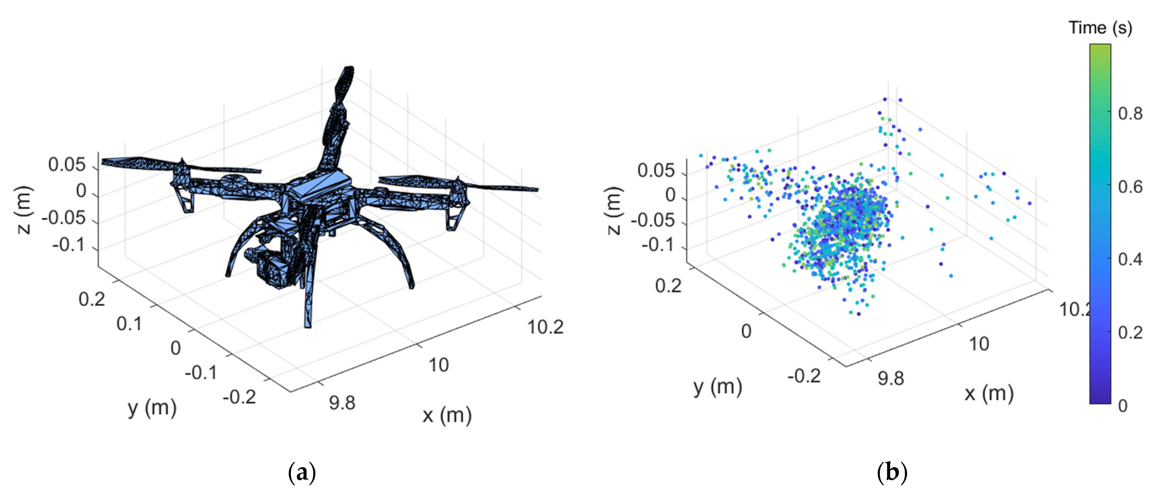
Figure 4 represents a stl model of a DJI F450 (Figure 4a), as well as a simulated point cloud at 10 m from the sensor for a sampling period of 1 s (Figure 4b). The points of the cloud are referenced with respect to the internal clock of the sensor, as can be seen in Figure 4b.
To estimate the position and speed of the obstacles in the scene, the on-board computer uses these distance measurements synchronized with the internal clock of the LiDAR and performs a linear regression to determine the position and speed of the obstacles (Equation (1)). They are samples taken randomly from different points on the surface of the stl model, so there will be a certain deviation in the measurements the sensor is measuring distances to different points of the surface. However, with a sample with enough points, this error can be eliminated statistically and positioning with centimeter precision can be achieved.
2.2. SOCP Collision Avoidance Algorithm
2.2.1. Navigation Environment of the UAV
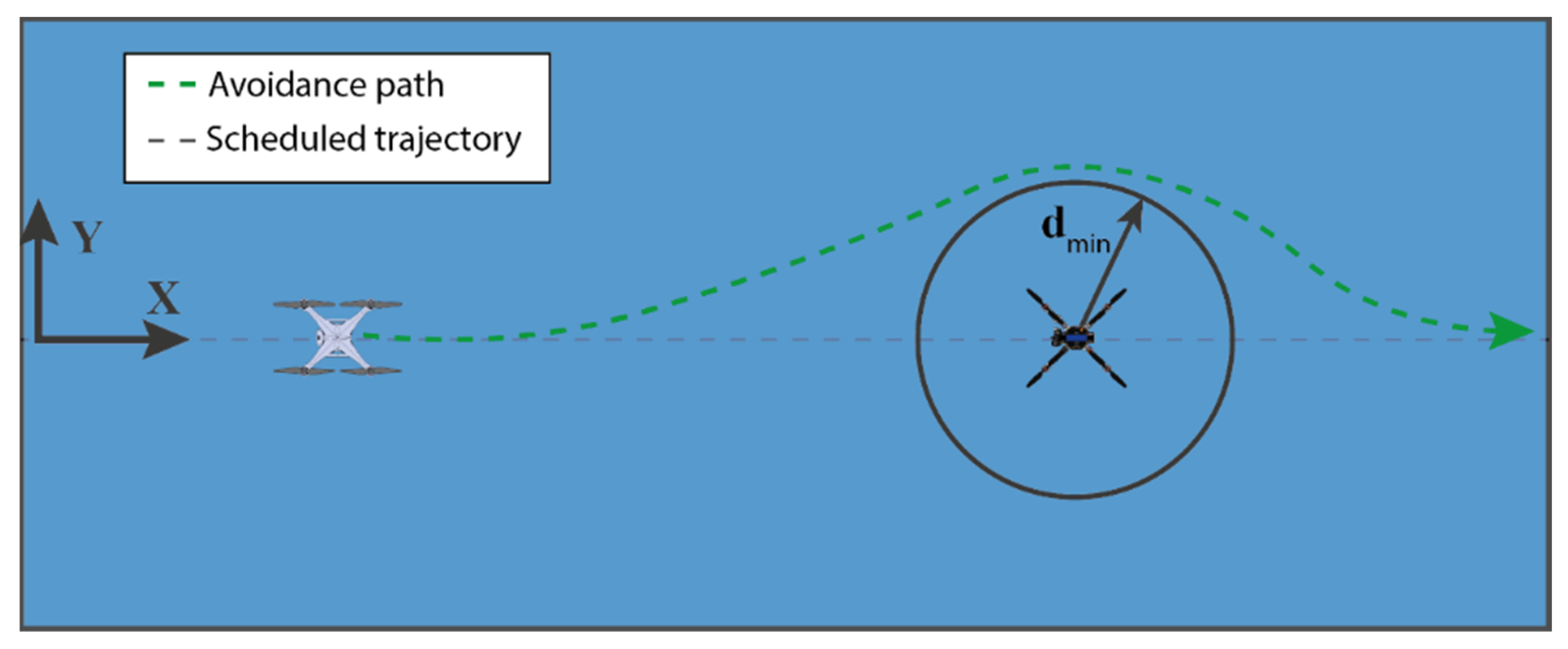
As aforementioned, the UAV’s navigation environment is a UAM corridor, which according to existing design concepts would be practically straight air highways free of obstacles. Nevertheless, it is likely that eventually flying objects such as unauthorized UAVs or birds will enter this airspace. To avoid the risk of collision, the aircraft must always maintain a lateral safety distance as shown in Figure 5. For this reason, the onboard computer computes in real time the probability of violating this distance restriction. It employs the predictions given by Equation (1) and activates the avoidance algorithm if necessary.
As was mentioned in the previous section, two reference frames were defined: the LiDAR and the global reference frame, being the latter the one used for the collision avoidance system. The position of the UAV in the UAM corridor is defined by a set of cartesian coordinates as can be seen in Figure 5. The X axis is aligned with the direction of the UAM corridor, while the Z coordinate represents the height of the aircraft. On the other hand, the Y coordinate measures the deviation with respect to the central line of the UAM corridor.
For the implementation of the obstacle avoidance algorithm based on SOCP (Second Order Cone Programming), the position of the UAV was discretized temporally and spatially. In this way, for a given number of discretization steps, the UAV state variables are defined through an array for the different instants of time (Equation (2)):
The execution of the maneuvers is executed in a period , which will depend on the distance travelled, as well as the complexity of the maneuver to be carried out. In this way the temporary array is defined as a function of . Thus, the vector t is defined as an array of equally spaced points by a time (Equation (3)):
To simplify the notation, from now on we will denote by the position of the aircraft in the Global Reference System at each time discretization step, according to Equation (4):
It is important to note that in this implementation, the position of the UAV was considered as the only state variable of the aircraft, which reduces the complexity of the problem and improves the SOCP computation times. To approximate the values of velocity and acceleration, first and second order finite differences were used, respectively, as described in Equation (5):
2.2.2. SOCP Formulation
SOCPs (Second Order Cone Programs) are convex optimization problems of a linear functional, in which the optimization variable is restricted to the region bounded by m cones in an Euclidean space (Equation (6)). Besides, there can also exist linear equalities among the components of the optimization variable, which are typically expressed in a matrix form.
where ∈ is the optimization variable. , , , , and are the optimization parameters. indicates the Euclidean norm.
The variable includes all the unknowns of the optimization problem. In the case of this obstacle avoidance algorithm, it will be equal to the UAV’s position vector at each discretization step, as well as the execution time of the maneuver () (Equation (7)). The variable is not included in the unknowns since it is not independent and can be calculated using Equation (3).
In the case of this obstacle avoidance problem, the function that was decided to be optimized is the flight time , in this way efficient routes are obtained that minimize the delay with respect to the originally planned route.
Regarding the equality constraints, the position and initial speed of the UAV are defined as the starting point of the algorithm. For the position, the numerical value is directly assigned to the optimization variables (Equation (8)), while for the velocity, finite differences (Equation (5)) were used to approximate the derivatives and operations were performed to obtain a linear system of equations (Equation (9)):
The final position of the UAV is defined through a quadratic inequality constraint (Equation (10)). The final position of the UAV is constrained to a sphere of radius , centered on the final point of the trajectory; this is to give some slack distance to the problem and speed up the convergence of the algorithm. In this way, the final position of the UAV is defined as:
The flight domain must be restricted to the limits of the UAM corridor. For this reason, to avoid that the UAV may escape from this region, linear inequality constraints are defined to establish the limits of the domain (Equation (11)). These constraints are applied in all the temporal steps of the maneuver, therefore:
For the correct execution of the maneuvers, the calculated routes must consider the operational characteristics of the aircraft. Additional constraints were added at each discretization step () to limit the maximum velocity and acceleration of the UAV. Regarding the speed limitation, as aforementioned, this quantity was approximated using finite differences. Deriving Equation (5), a conic inequality constrained was obtained to limit the maximum speed (Equation (12)).
Equivalently, for the acceleration, the same procedure was followed to obtain Equation (13). However, this expression is not conic, as a appears outside the Euclidean norm term:
In order to obtain a conic constraint, the right-hand side of Equation (13) was linearized with a Taylor expansion (Equation (14)) to obtain an expression in the standard form of a SOCP. The linearization was carried out around a reference value (. This quantity is equal to the expected time of flight for a straight path between the start and end points, divided by . Finally, after this relaxation, Equation (15) was obtained:
The last restriction for calculating trajectories is the minimum lateral safety distance with respect to the different obstacles in the navigation environment (. To introduce the position of the obstacles to the SOCP algorithm, Equation (1) was discretized in the temporal array obtaining Equation (16):
Thus, with this discretization and the position of the UAV, the minimum lateral separation is defined in Equation (17):
Finally, all these equations are converted into the standard form of a SOCP and solved using a large-scale optimizer. To accelerate the convergence of the calculations, a straight trajectory at the maximum possible speed between the initial and final point of the UAV’s trajectory is introduced as an initial guess to the solver. In this work, three large-scale optimizers were used to compare their relative performance: SNOPT [23], IPOPT [22], and KNITRO [24].
3. Results
3.1. LiDAR System Detection Capabilities
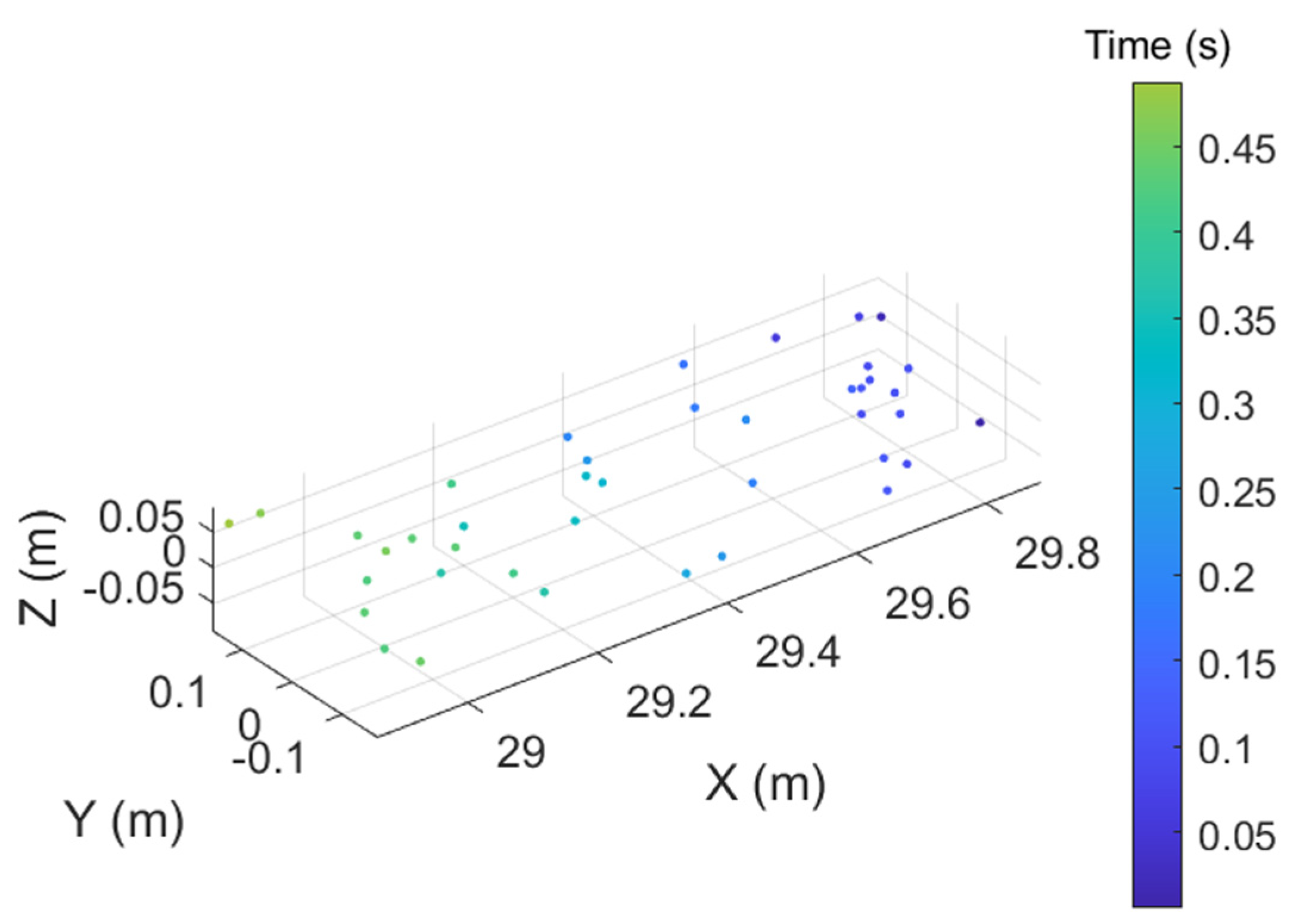
To validate the positioning capabilities of the linear regression method presented in Equation (1), several scenarios of a target approaching the sensor at different speeds and from different distances were simulated. To do this, a stl model of a DJI F450 was sampled for 0.5 s and point clouds such as the one represented in Figure 6 were obtained. As can be seen, the point density of this cloud is much lower than the one of Figure 4b since it was acquired at a greater distance and with a shorter sampling period. The device works as if it were a rangefinder, that takes random points from the surface of a body to make estimations of its position.
Table 2 shows the results of the regression along with the 95% confidence interval for the different scenarios. As can be seen, the errors are of the order of cm for both the speed and the ordinate at the origin. It is an acceptable result considering the precision of the instrument and the low density of points. For the distance of 30 m, the precision was slightly lower since fewer points were obtained. It can also be seen that the sensor tends to position the target slightly closer to its actual center of mass position. This is because most of the captured points, due to the sensor’s field of view, correspond to the front of the DJI F450.
3.2. Avoidance Maneuvers
To study the capabilities of the Detect and Avoid algorithm, several test cases were defined for a quadcopter with a maximum speed limited to 5 m/s and a maximum acceleration of 2 m/s. This UAV flies between two waypoints of the UAM corridor, being the start point (0, 0) and the end point (50, 50). During the trajectory, different invading aircraft penetrate the airspace and violate the minimum separation distance restrictions. The UAV must first detect these aircraft, to later estimate their position and make the appropriate trajectory corrections. For this purpose, the stl model of the DJI F450 and a sampling period of 0.5 s were used for the regression.
A minimum safety distance of 5 m was used for all study cases. The on-board computer every 0.5 s performs the linear regression and estimates the trajectory of the invading aircraft. If it detects that the safety distance may be smaller than 4.5 m for any point of the trajectory, the SOCP algorithm is activated, and the trajectory is recalculated. The number of discretization points was adapted dynamically for each maneuver considering the distance in a straight line from the initial point to the end of the trajectories, adapting this parameter to have one discretization point per meter of distance. To better understand how avoidance maneuvers are performed, videos of the study cases were included in the Supplementary Materials section. For each study case, animations of the trajectories as well as the dynamic point clouds sampled by the LiDAR sensor are provided.
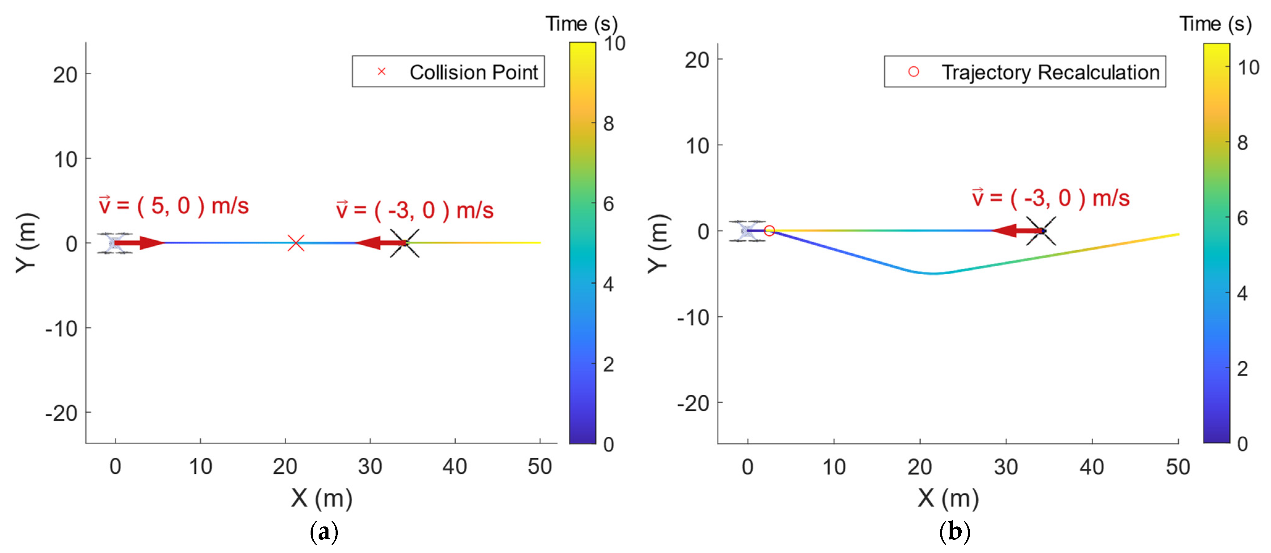
3.2.1. Colinear Obstacle
In this first case study, the UAV flies at a speed of 5 m/s and encounters an intruder approaching towards it at a speed of 3 m/s. Both aircraft, if they continue with their trajectories, will collide head-on, as shown in Figure 7a. Figure 7b shows the simulated avoidance trajectory. Firstly, the UAV samples the position of the intruder, and during this time it moves 2.5 m. Then, the SOCP algorithm is activated, and an avoidance maneuver is calculated to maintain the lateral separation and avoid the collision. During this simulation, the trajectories of the UAV were not recalculated since the intruder did not change, it remained at a constant speed.
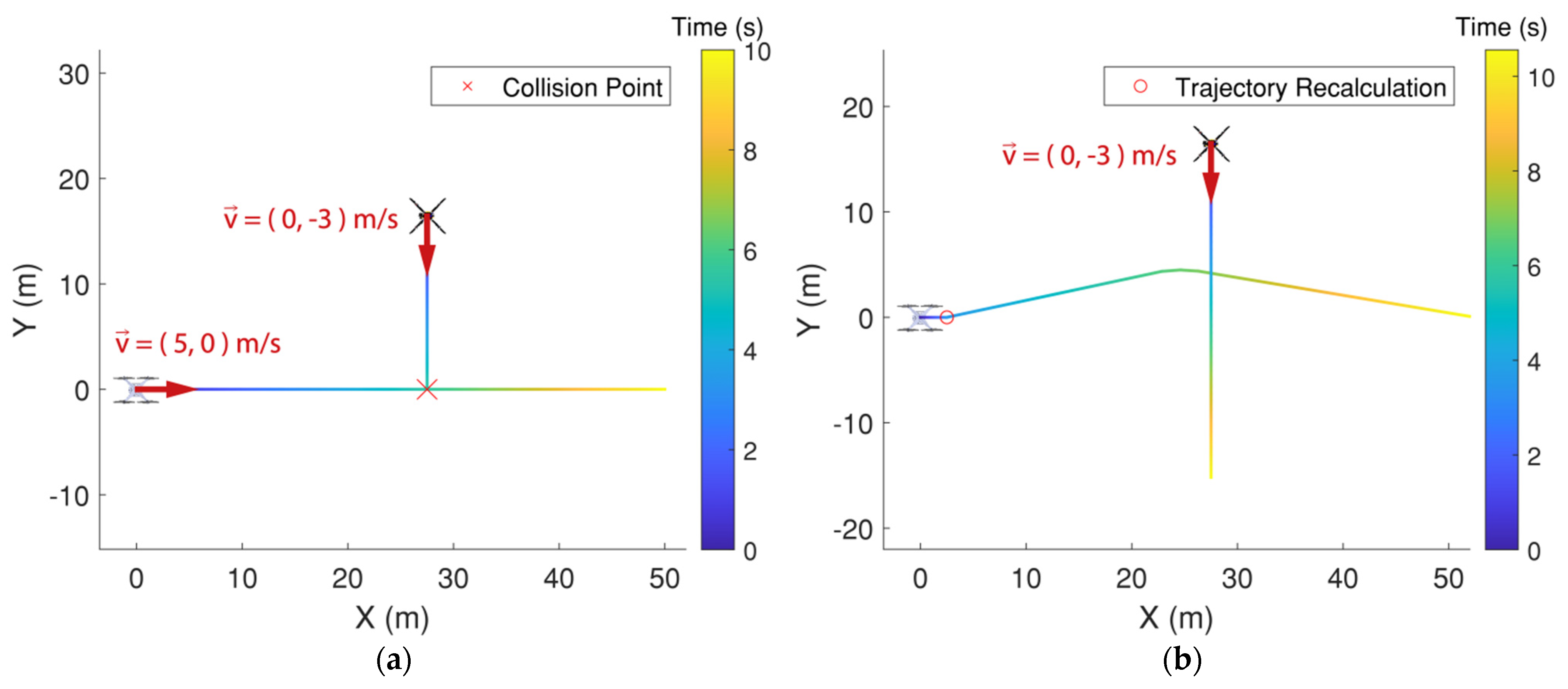
3.2.2. Perpendicular Obstacle
In this second case study, the UAV flying at 5 m/s encounters an obstacle that is flying at 3 m/s in a direction perpendicular to it. According to the trajectories of both, if no action is taken, both will collide sideways, as shown in Figure 8a. Figure 8b shows the simulation results. As in the previous case, firstly, the UAV samples the position of the intruder to then proceed to calculate the evasion maneuver shown in the figure. As in the previous case, the algorithm did not need to recalculate the aircraft’s trajectory as the intruder kept flying at the same constant speed.
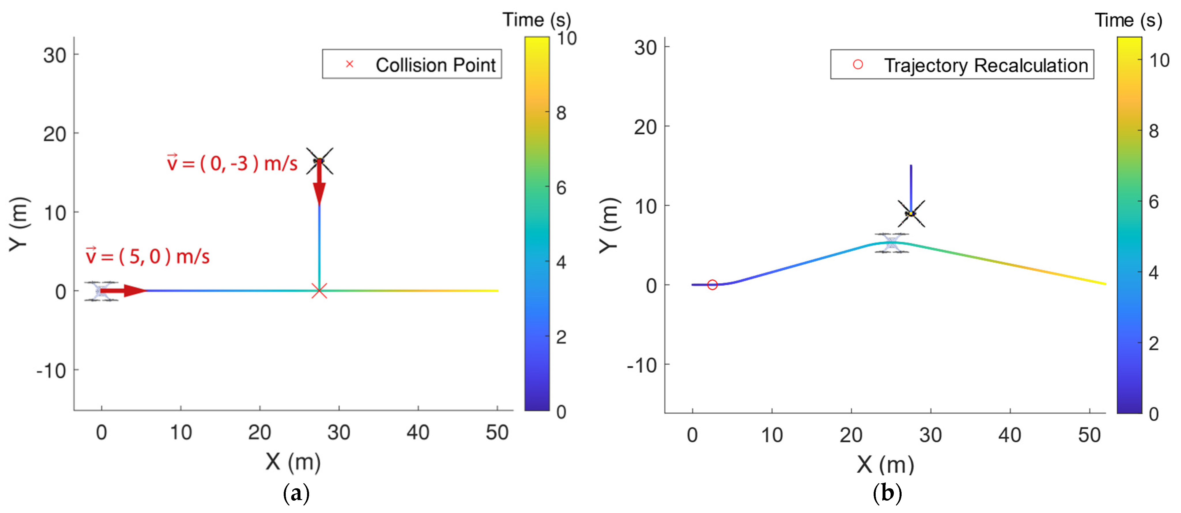
3.2.3. Obstacle with Acceleration
The following case study is similar to the one shown in Section 3.2.2, in which an obstacle moving at 3 m/s is directed towards the UAV perpendicularly (Figure 9a). However, in this case, the obstacle decides to brake by applying a constant acceleration of 1 m/s2 to avoid the collision. After this change in the trajectory of the obstacle, if the UAV were to perform the maneuver calculated in Section 3.2.2, it would violate the minimum safety distance as represented in (Figure 9b).
In this maneuver, the system, which constantly updates the predictions of the motion of the obstacle, computes two trajectory changes as shown in Figure 10. Firstly, as in Section 3.2.2, it moves towards positive values of Y to avoid the obstacle, but when it detects that the obstacle decelerates, it recalculates a new trajectory to avoid it. As can be seen, the safety distance applied is greater than the minimum, since when it performs the second trajectory calculation, the intruder obstacle is at a speed of 2 m/s heading towards the UAV. After calculating this trajectory, the intruder continues to decrease its speed, but no further route changes are made since there is no risk of collision.
3.2.4. Dynamic Scenario
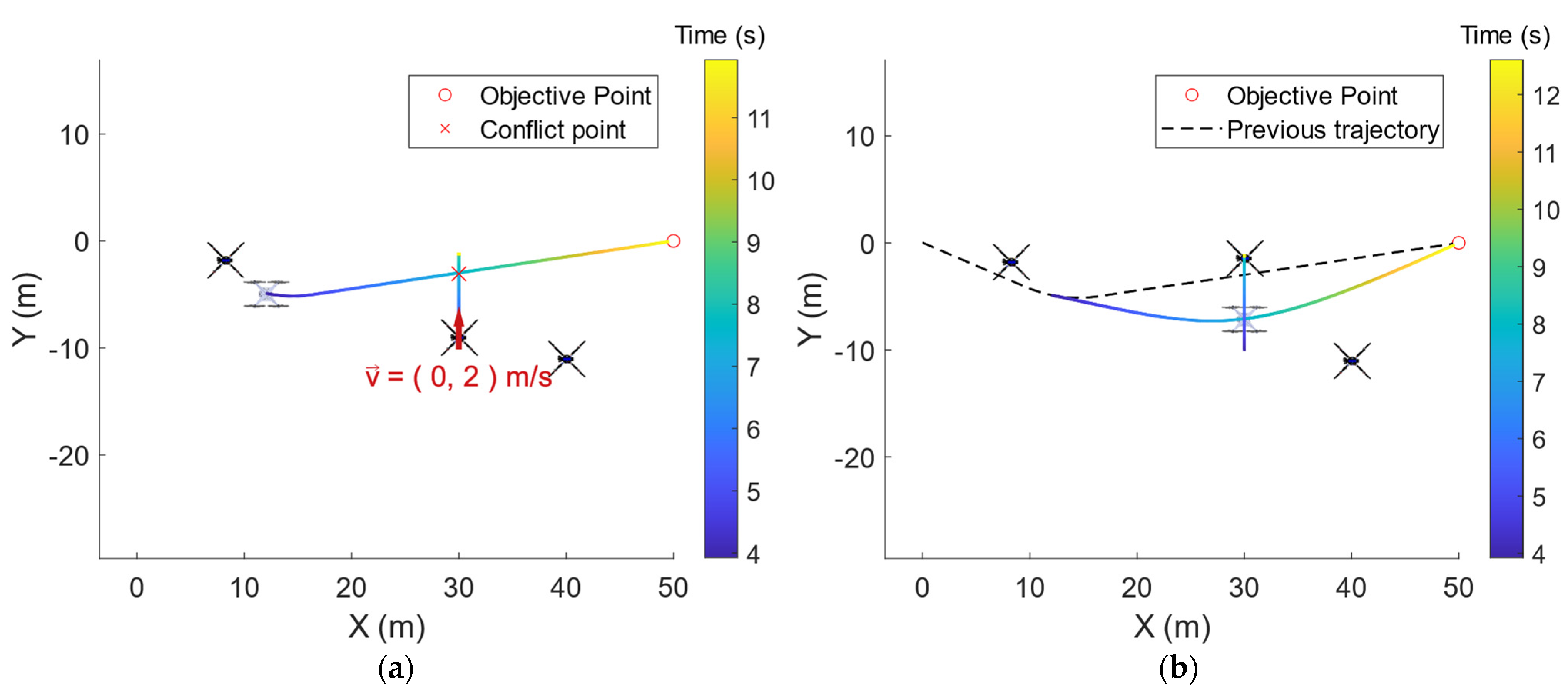
In this last maneuver, a scenario with various obstacles with changing speeds was simulated, for which the UAV must recalculate its trajectory dynamically. The UAV is hovering at the initial point and detects the presence of three intruders. One of them moving diagonally and the others fixed in their initial position (Figure 11a). After sampling their positions, it executes the maneuver depicted in Figure 11b.
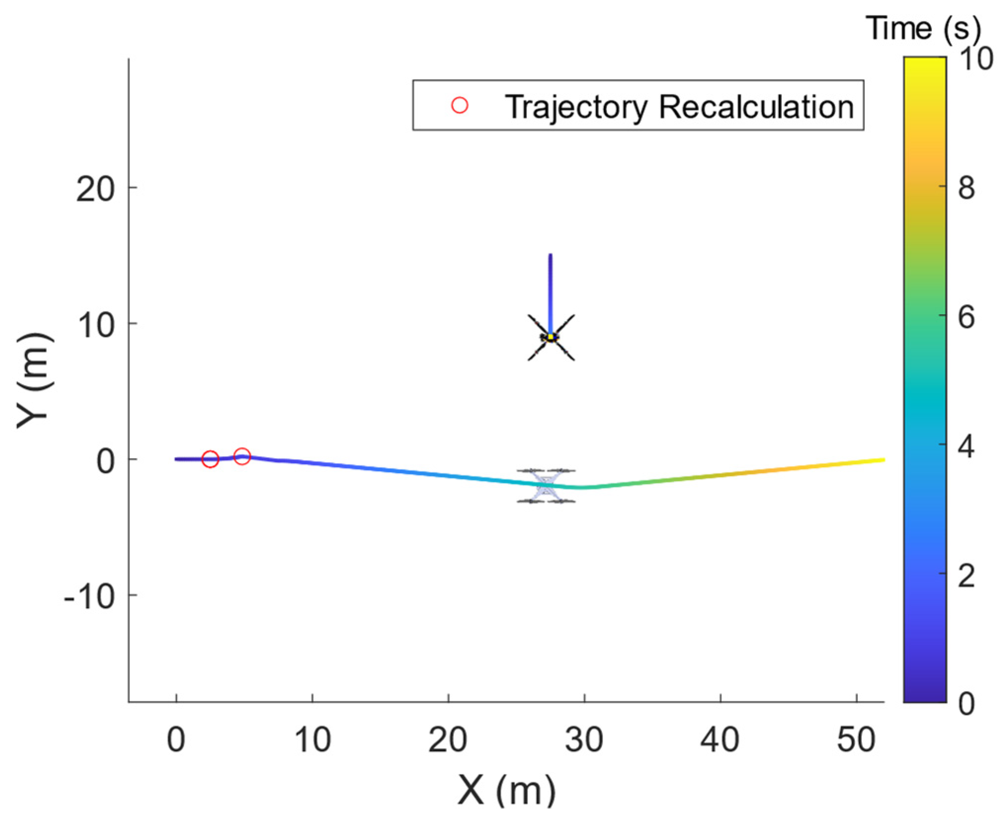
During the execution of the trajectory, four seconds after its beginning, the second obstacle begins to move in the direction of the Y axis, approaching the calculated trajectory of the UAV. After performing the sampling, the on-board computer recalculates the trajectory and performs the arc represented in Figure 12.
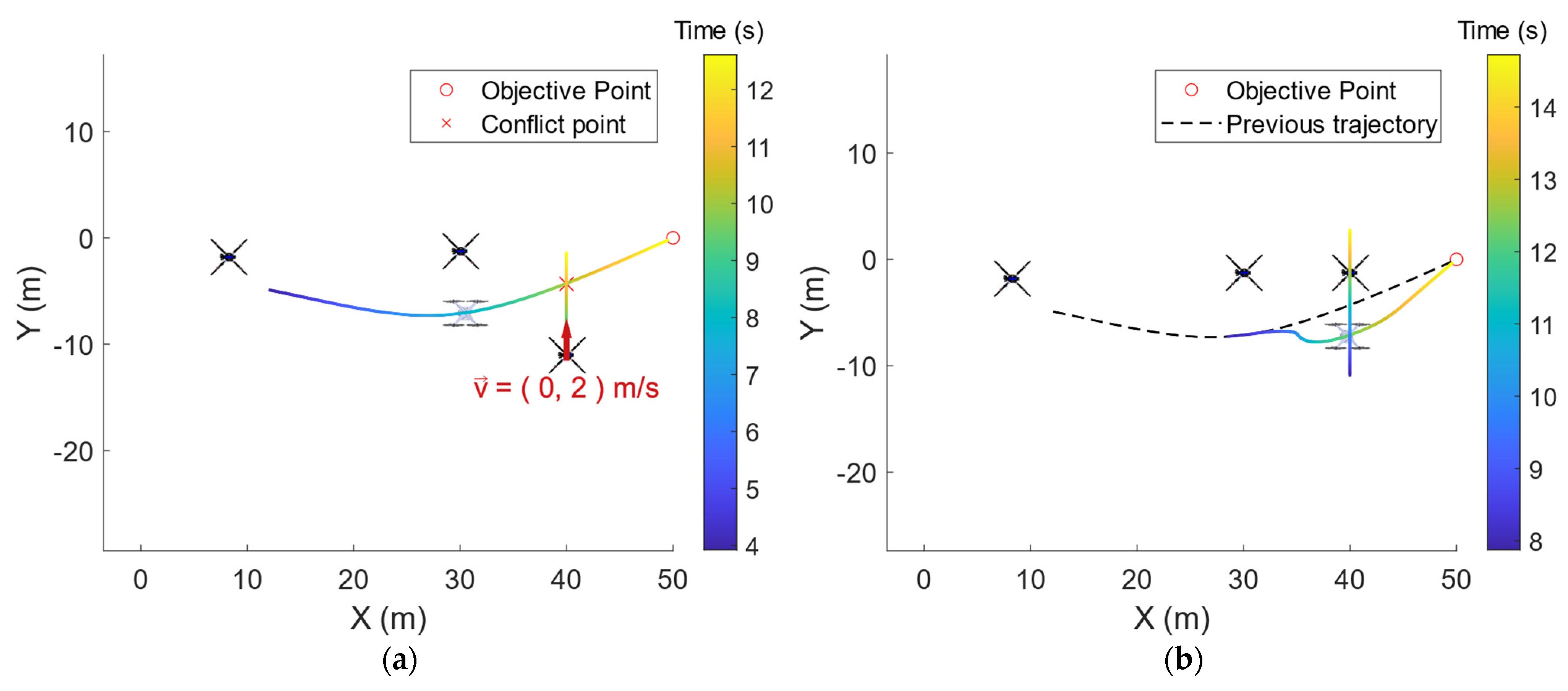
Consequently, when the aircraft is close to the point X = 30 m, the third obstacle starts to move towards the UAV, as shown in Figure 13a. The UAV then reduces its speed and performs the maneuver shown in Figure 13b to maintain the safety distance and reach the final point.
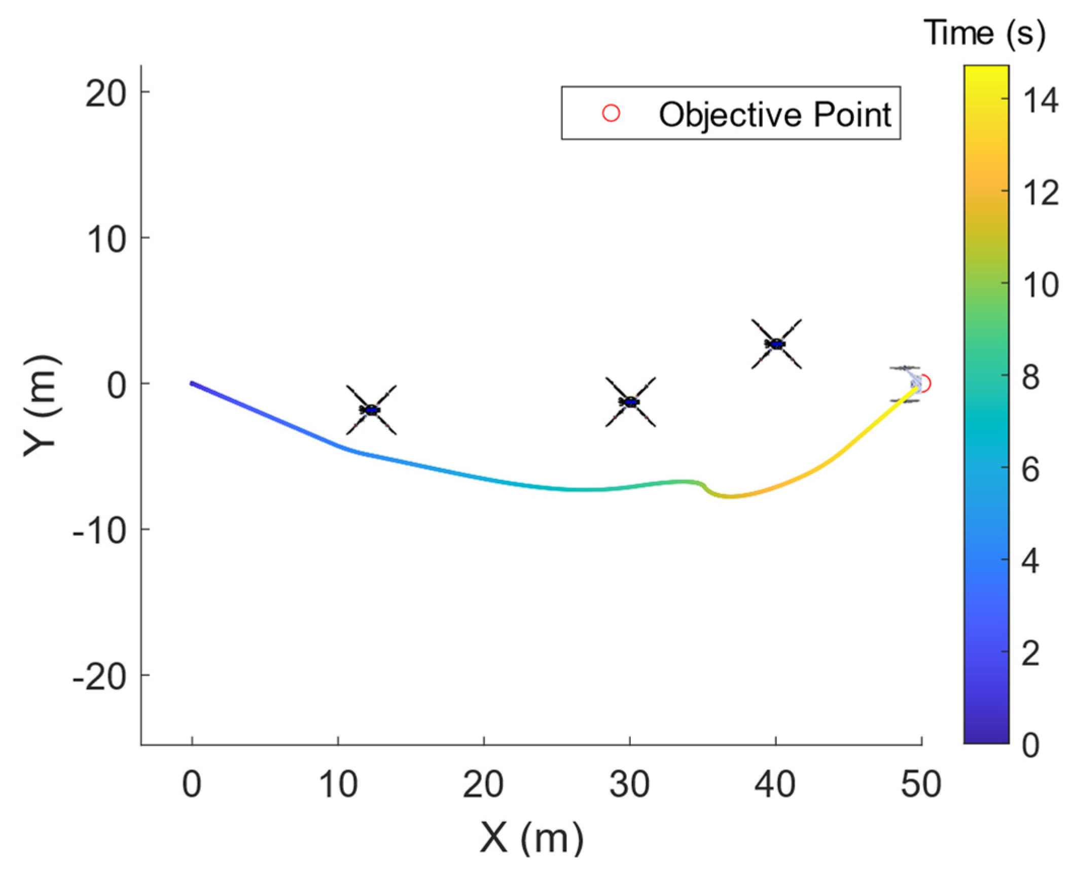
Finally, in Figure 14 the trajectory followed by the UAV is presented after the two trajectory recalculations.
3.3. Computation Time
All the previous simulations were carried out on a laptop using an AMD Ryzen 5 3500U processor. The computation time was measured using different solvers for quadratic and nonlinear optimization problems. Table 3 presents the results for all the maneuvers computed in this work. The first two study cases only required the calculation of a trajectory since the speed of the intruders did not vary throughout the simulation. For the third study case, two additional maneuvers were calculated for which 39 and 22 discretization points were used, respectively. For all the maneuvers, quite low calculation times were obtained with the three solvers, which would allow real-time implementation on an on-board computer. Overall, the KNITRO optimizer had the best performance of the three, closely followed by SNOPT.
4. Conclusions
This article presents a Detect and Avoid solution for UAV navigation in UAM corridors. A commercial LiDAR sensor was simulated including its operational characteristics to replicate the detection capabilities that an UAV would have with this technology. With this information, an avoidance algorithm based on SOCP programming was developed to compute trajectories in real time and modify the trajectory of the vehicle if a risk of collision is anticipated. The following goals were achieved:
- The position and speed of the obstacles were correctly measured employing the point clouds from the LiDAR sensor.
- UAV operational characteristics are considered for the computation of trajectories.
- A fast implementation was obtained that allows the calculation of trajectories practically in real time on a modern computer.
In future works, the effect of meteorological phenomena such as wind gusts on the evasion capabilities of the algorithm will be studied. The influence of the speed and size of the intruders will be analyzed to evaluate how the safety distance should be dynamically adapted with respect to them. In addition, the feasibility of adapting this implementation or developing a new methodology for fixed-wing aircraft will also be assessed.
Supplementary Materials
The following supporting information can be downloaded at: https://0-www-mdpi-com.brum.beds.ac.uk/article/10.3390/drones6080185/s1, Video S1: Study Case 3.2.1: Colinear obstacle avoidance; Video S2: Study Case 3.2.1: Colinear obstacle avoidance (Point clouds); Video S3: Study Case 3.2.2: Perpendicular obstacle avoidance; Video S4: Study Case 3.2.2: Perpendicular obstacle avoidance (Point clouds); Video S5: Study Case 3.2.3: Obstacle with acceleration; Video S6: Study Case 3.2.3: Obstacle with acceleration (Point clouds); Video S7: Study Case 3.2.4: Dynamic obstacle avoidance; Video S8: Study Case 3.2.4: Dynamic obstacle avoidance (Point clouds).
Author Contributions
Conceptualization, E.A., L.M.G.-d.S. and H.G.-J.; Investigation, E.A.; Methodology, E.A., L.M.G.-d.S. and H.G.-J.; Software, E.A.; Supervision, L.M.G.-d.S. and H.G.-J.; Writing—original draft, E.A.; Writing—review and editing, L.M.G.-d.S. and H.G.-J. All authors have read and agreed to the published version of the manuscript.
Funding
L.M.G.-d. is funded by the Recovery, Transformation and Resilience Plan of the European Union—NextGenerationEU (University of Vigo grant ref. 585507).
Institutional Review Board Statement
Not Applicable.
Informed Consent Statement
Not Applicable.
Data Availability Statement
The data used in this study are not publicly available due to the conditions of the ethics approval for the study. Contact the corresponding author for further information.
Acknowledgments
Authors would like to thank the University of Vigo for the support and resources provided for the realization of this work.
Conflicts of Interest
The authors declare no conflict of interest.
References
- SESAR Joint Undertaking|U-Space. Available online: https://www.sesarju.eu/U-space (accessed on 16 June 2022).
- U-Space Blueprint. Available online: https://www.sesarju.eu/sites/default/files/documents/reports/U-space%20Blueprint%20brochure%20final.PDF (accessed on 22 June 2022).
- EASA Concept of Operations for Drones. Available online: https://www.easa.europa.eu/sites/default/files/dfu/204696_EASA_concept_drone_brochure_web.pdf (accessed on 20 June 2022).
- Barrado, C.; Boyero, M.; Brucculeri, L.; Ferrara, G.; Hately, A.; Hullah, P.; Martin-Marrero, D.; Pastor, E.; Rushton, A.P.; Volkert, A. U-Space Concept of Operations: A Key Enabler for Opening Airspace to Emerging Low-Altitude Operations. Aerospace 2020, 7, 24. [Google Scholar] [CrossRef] [Green Version]
- Bradford, S. Concept of Operations for Urban Air Mobility. Fed. Aviat. Adm. NextGen Off. 2020, 6, 26. Available online: https://nari.arc.nasa.gov/sites/default/files/attachments/UAM_ConOps_v1.0.pdf (accessed on 21 July 2022).
- Bauranov, A.; Rakas, J. Designing Airspace for Urban Air Mobility: A Review of Concepts and Approaches. Prog. Aerosp. Sci. 2021, 125, 100726. [Google Scholar] [CrossRef]
- K-UAM Grand Challenge. Available online: http://en.kuam-gc.kr/ (accessed on 22 June 2022).
- Garrow, L.A.; German, B.J.; Leonard, C.E. Urban Air Mobility: A Comprehensive Review and Comparative Analysis with Autonomous and Electric Ground Transportation for Informing Future Research. Transp. Res. Part C Emerg. Technol. 2021, 132, 103377. [Google Scholar] [CrossRef]
- Dziugiel, B.; Mazur, A.; Stanczyk, A.; Maczka, M.; Liberacki, A.; di Vito, V.; Menichino, A.; Melo, S.; ten Thije, J.; Hesselink, H.; et al. Acceptance, Safety and Sustainability Recommendations for Efficient Deployment of UAM–Outline of H2020 CSA Project. IOP Conf. Ser. Mater. Sci. Eng. 2022, 1226, 012082. [Google Scholar] [CrossRef]
- Pongsakornsathien, N.; Bijjahalli, S.; Gardi, A.; Symons, A.; Xi, Y.; Sabatini, R.; Kistan, T. A Performance-Based Airspace Model for Unmanned Aircraft Systems Traffic Management. Aerospace 2020, 7, 154. [Google Scholar] [CrossRef]
- Semke, W.; Allen, N.; Tabassum, A.; McCrink, M.; Moallemi, M.; Snyder, K.; Arnold, E.; Stott, D.; Wing, M.G. Analysis of Radar and ADS-B Influences on Aircraft Detect and Avoid (DAA) Systems. Aerospace 2017, 4, 49. [Google Scholar] [CrossRef] [Green Version]
- Lippitsch, G. Detect and Avoid Remotely Piloted Aircraft Systems Symposium. 2015. Available online: https://www.icao.int/Meetings/RPAS/RPASSymposiumPresentation/Day%202%20Workshop%205%20Technology%20Gerhard%20Lippitsch%20-%20Detect%20and%20Avoid.pdf (accessed on 21 July 2022).
- Li, Y.; Ibanez-Guzman, J. Lidar for Autonomous Driving: The Principles, Challenges, and Trends for Automotive Lidar and Perception Systems. IEEE Signal Process. Mag. 2020, 37, 50–61. [Google Scholar] [CrossRef]
- Raj, T.; Hashim, F.H.; Huddin, A.B.; Ibrahim, M.F.; Hussain, A. A Survey on LiDAR Scanning Mechanisms. Electron 2020, 9, 741. [Google Scholar] [CrossRef]
- Royo, S.; Ballesta-Garcia, M. An Overview of Lidar Imaging Systems for Autonomous Vehicles. Appl. Sci. 2019, 9, 4093. [Google Scholar] [CrossRef] [Green Version]
- Möller, T.; Trumbore, B. Fast, Minimum Storage Ray-Triangle Intersection. J. Graph. Tools 1997, 2, 21–28. [Google Scholar] [CrossRef]
- Boyd, S.; Vandenberghe, L. Convex Optimization; Cambridge University Press: Cambridge, UK, 2004. [Google Scholar]
- Aldao, E.; González-Desantos, L.M.; Michinel, H.; González-Jorge, H. UAV Obstacle Avoidance Algorithm to Navigate in Dynamic Building Environments. Drones 2022, 6, 16. [Google Scholar] [CrossRef]
- Fu, C.; Olivares-Mendez, M.A.; Suarez-Fernandez, R.; Campoy, P. Monocular Visual-Inertial SLAM-Based Collision Avoidance Strategy for Fail-Safe UAV Using Fuzzy Logic Controllers: Comparison of Two Cross-Entropy Optimization Approaches. J. Intell. Robot. Syst. Theory Appl. 2014, 73, 513–533. [Google Scholar] [CrossRef] [Green Version]
- Sathya, A.; Sopasakis, P.; van Parys, R.; Themelis, A.; Pipeleers, G.; Patrinos, P. Embedded Nonlinear Model Predictive Control for Obstacle Avoidance Using PANOC. In Proceedings of the 2018 European Control Conference, Limassol, Cyprus, 12–15 June 2018. [Google Scholar] [CrossRef] [Green Version]
- Lindqvist, B.; Mansouri, S.S.; Agha-Mohammadi, A.A.; Nikolakopoulos, G. Nonlinear MPC for Collision Avoidance and Control of UAVs with Dynamic Obstacles. IEEE Robot. Autom. Lett. 2020, 5, 6001–6008. [Google Scholar] [CrossRef]
- Wächter, A.; Biegler, L.T. On the Implementation of an Interior-Point Filter Line-Search Algorithm for Large-Scale Nonlinear Programming. Math. Program. 2006, 106, 25–57. [Google Scholar] [CrossRef]
- Gill, P.E.; Murray, W.; Saunders, M.A. SNOPT: An SQP Algorithm for Large-Scale Constrained Optimization. Soc. Ind. Appl. Math. 2005, 47, 99–131. [Google Scholar] [CrossRef]
- Byrd, R.H.; Nocedal, J.; Waltz, R.A. Knitro: An Integrated Package for Nonlinear Optimization; Springer: Boston, MA, USA, 2006. [Google Scholar] [CrossRef]
- Guo, J.; Liang, C.; Wang, K.; Sang, B.; Wu, Y. Three-Dimensional Autonomous Obstacle Avoidance Algorithm for UAV Based on Circular Arc Trajectory. Int. J. Aerosp. Eng. 2021, 2021, 8819618. [Google Scholar] [CrossRef]
- Wang, C.; Savkin, A.V.; Garratt, M. A Strategy for Safe 3D Navigation of Non-Holonomic Robots among Moving Obstacles. Robotica 2018, 36, 275–297. [Google Scholar] [CrossRef]
- Liu, Z.; Zhang, Y.; Yuan, C.; Ciarletta, L.; Theilliol, D. Collision Avoidance and Path Following Control of Unmanned Aerial Vehicle in Hazardous Environment. J. Intell. Robot. Syst. Theory Appl. 2019, 95, 193–210. [Google Scholar] [CrossRef]
- Aniceto1, S.B.P.; McGrah, R.V.S.; Ochengco, C.J.I.; Regalado, M.G.; Chua, A.Y. A Novel Low-Cost Obstacle Avoidance System for a Quadcopter UAV Using Fuzzy Logic. Int. J. Mech. Eng. Robot. Res. 2020, 9, 733. [Google Scholar] [CrossRef]
- Budiyanto, A.; Cahyadi, A.; Adji, T.B.; Wahyunggoro, O. UAV Obstacle Avoidance Using Potential Field under Dynamic Environment. In Proceedings of the ICCEREC 2015–International Conference on Control, Electronics, Renewable Energy and Communications, Bandung, Indonesia, 27–29 August 2015. [Google Scholar] [CrossRef]
- Du, Y.; Zhang, X.; Nie, Z. A Real-Time Collision Avoidance Strategy in Dynamic Airspace Based on Dynamic Artificial Potential Field Algorithm. IEEE Access 2019, 7, 169469–169479. [Google Scholar] [CrossRef]
- Kownacki, C.; Ambroziak, L. A New Multidimensional Repulsive Potential Field to Avoid Obstacles by Nonholonomic Uavs in Dynamic Environments. Sensors 2021, 21, 7495. [Google Scholar] [CrossRef]
- Lee, H.Y.; Ho, H.W.; Zhou, Y. Deep Learning-Based Monocular Obstacle Avoidance for Unmanned Aerial Vehicle Navigation in Tree Plantations: Faster Region-Based Convolutional Neural Network Approach. J. Intell. Robot. Syst. Theory Appl. 2021, 101, 5. [Google Scholar] [CrossRef]
- Back, S.; Cho, G.; Oh, J.; Tran, X.T.; Oh, H. Autonomous UAV Trail Navigation with Obstacle Avoidance Using Deep Neural Networks. J. Intell. Robot. Syst. Theory Appl. 2020, 100, 1195–1211. [Google Scholar] [CrossRef]
- Wang, Z.; Xu, G.; Liu, L.; Long, T. Obstacle-Avoidance Trajectory Planning for Attitude-Constrained Quadrotors Using Second-Order Cone Programming. In Proceedings of the 2018 Aviation Technology, Integration, and Operations Conference. [CrossRef]
- Zhong, K.; Jain, P.; Kapoor, A. Fast Second-Order Cone Programming for Safe Mission Planning. In Proceedings of the Proceedings–IEEE International Conference on Robotics and Automation, Singapore, 29 May–3 June 2017. [Google Scholar] [CrossRef] [Green Version]
- Szmuk, M.; Pascucci, C.A.; Dueri, D.; Acikmese, B. Convexification and Real-Time on-Board Optimization for Agile Quad-Rotor Maneuvering and Obstacle Avoidance. In Proceedings of the IEEE International Conference on Intelligent Robots and Systems, Vancouver, BC, Canada, 24–28 September 2017; Volume 2017. [Google Scholar] [CrossRef]
- Zhang, G.; Kuang, H.; Liu, X. Fast Trajectory Optimization for Quadrotor Landing on a Moving Platform. In Proceedings of the 2020 International Conference on Unmanned Aircraft Systems, Athens, Greece, 1–4 September 2020. [Google Scholar] [CrossRef]
- Shen, Z.; Yu, J.; Dong, X.; Hua, Y.; Ren, Z. Penetration Trajectory Optimization for the Hypersonic Gliding Vehicle Encountering Two Interceptors. Aerosp. Sci. Technol. 2022, 121, 107363. [Google Scholar] [CrossRef]
- Tang, M.; He, Q.; Luo, X.; Liu, L.; Wang, Y.; Cheng, Z. Reentry Trajectory Optimization Based on Second Order Cone Programming. In Proceedings of the 32nd Chinese Control and Decision Conference, Hefei, China, 22–24 August 2020. [Google Scholar] [CrossRef]
- Kwon, H.H.; Choi, H.L. A Convex Programming Approach to Mid-Course Trajectory Optimization for Air-to-Ground Missiles. Int. J. Aeronaut. Space Sci. 2020, 21, 479–492. [Google Scholar] [CrossRef]
- Wang, H.; Zhang, H.; Wang, Z.; Guan, Y. An Optimal Trajectory Design for Lunar Surface Hop. Zhongguo Kongjian Kexue Jishu/Chin. Space Sci. Technol. 2021, 41, 112. [Google Scholar] [CrossRef]
- Szmuk, M.; Eren, U.; Açıkmeşe, B. Successive Convexification for Mars 6-DoF Powered Descent Landing Guidance. In Proceedings of the AIAA Guidance, Navigation, and Control Conference, Grapevine, TX, USA, 9–13 January 2017. [Google Scholar]
- Chen, X.; Cao, R.; Hu, Q. Spacecraft Attitude Control with Saturation and Attitude Forbidden Constraints via Second-Order Cone Programming. Trans. Nanjing Univ. Aeronaut. Astronaut. 2021, 38, 237–248. [Google Scholar] [CrossRef]
- Szmuk, M.; Açıkmeşe, B. Successive Convexification for 6-DoF Mars Rocket Powered Landing with Free-Final-Time. In Proceedings of the AIAA Guidance, Navigation, and Control Conference, Kissimmee, FL, USA, 8–12 January 2018. [Google Scholar] [CrossRef] [Green Version]
- Specs–Avia LiDAR Sensor–Livox. Available online: https://www.livoxtech.com/avia/specs (accessed on 22 June 2022).
Figure 1.
Workflow diagram.

Figure 2.
Experimental scanning pattern of the Livox Avia sensor.

Figure 3.
LiDAR Sensor Simulation.

Figure 4.
Reference model and simulation: (a) Original stl mesh. (b) Simulated point cloud.

Figure 5.
UAM Corridor environment.

Figure 6.
Sampled dynamic point cloud.

Figure 7.
Colinear obstacle avoidance maneuver: (a) Scheduled trajectory. (b) Recalculated path.

Figure 8.
Perpendicular obstacle avoidance maneuver: (a) Scheduled trajectory. (b) Recalculated path.
Figure 8.
Perpendicular obstacle avoidance maneuver: (a) Scheduled trajectory. (b) Recalculated path.

Figure 9.
Accelerating obstacle avoidance maneuver: (a) Initial forecasted obstacle trajectory. (b) Initial avoidance maneuver.
Figure 9.
Accelerating obstacle avoidance maneuver: (a) Initial forecasted obstacle trajectory. (b) Initial avoidance maneuver.

Figure 10.
Avoidance trajectory.

Figure 11.
Dynamic scenario avoidance maneuver 1: (a) Scheduled trajectory. (b) Recalculated path.

Figure 12.
Dynamic scenario avoidance maneuver 2: (a) Scheduled trajectory. (b) Recalculated path.

Figure 13.
Dynamic scenario avoidance maneuver 3: (a) Scheduled trajectory. (b) Recalculated path.

Figure 14.
Final trajectory.


Table 1.
Livox Avia Specifications.
| Characteristic | Specification |
|---|---|
| Detection Range (@100 klx) | 190 m @ 10% reflectivity |
| 230 m @ 20% reflectivity | |
| 320 m @ 80% reflectivity | |
| Field of view | 70.4° (Horizontal) × 77.2° (Vertical) |
| Range Precision (1σ @ 20 m) | 2 cm |
| Point Rate | 240,000 pts/s |
| Weight | 498 g |
| Dimensions | 91 × 61.2 × 64.8 mm |
Table 2.
Linear regression results.
| Distance (m) | Real Speed (m/s) | ||
|---|---|---|---|
| 10 | −2 | 9.94 ± 0.03 | −2.01 ± 0.02 |
| 10 | −5 | 9.94 ± 0.03 | −5.00 ± 0.05 |
| 10 | −10 | 9.96 ± 0.03 | −9.96 ± 0.05 |
| 30 | −2 | 29.95 ± 0.03 | −2.06 ± 0.13 |
| 30 | −5 | 29.97 ± 0.03 | −5.03 ± 0.14 |
| 30 | −10 | 29.95 ± 0.03 | −10.02 ± 0.12 |
Table 3.
Linear regression results.
| Study Case | Discretization Steps | Solver | Computation Time (s) |
|---|---|---|---|
| Colinear Obstacle | IPOPT | 0.11 | |
| 50 | SNOPT | 0.07 | |
| KNITRO | 0.04 | ||
| Perpendicular Obstacle | IPOPT | 0.05 | |
| 50 | SNOPT | 0.04 | |
| KNITRO | 0.03 | ||
| Obstacle with acceleration | IPOPT | 0.04 | |
| 50 | SNOPT | 0.03 | |
| KNITRO | 0.03 | ||
| Dynamic Scenario (First maneuver) | IPOPT | 0.08 | |
| 50 | SNOPT | 0.04 | |
| KNITRO | 0.04 | ||
| Dynamic Scenario (Second maneuver) | IPOPT | 0.05 | |
| 39 | SNOPT | 0.03 | |
| KNITRO | 0.03 | ||
| Dynamic Scenario (Third maneuver) | IPOPT | 0.04 | |
| 22 | SNOPT | 0.03 | |
| KNITRO | 0.03 |
Publisher’s Note: MDPI stays neutral with regard to jurisdictional claims in published maps and institutional affiliations. |
© 2022 by the authors. Licensee MDPI, Basel, Switzerland. This article is an open access article distributed under the terms and conditions of the Creative Commons Attribution (CC BY) license (https://creativecommons.org/licenses/by/4.0/).
Share and Cite
MDPI and ACS Style
Aldao, E.; González-de Santos, L.M.; González-Jorge, H. LiDAR Based Detect and Avoid System for UAV Navigation in UAM Corridors. Drones 2022, 6, 185. https://0-doi-org.brum.beds.ac.uk/10.3390/drones6080185
AMA Style
Aldao E, González-de Santos LM, González-Jorge H. LiDAR Based Detect and Avoid System for UAV Navigation in UAM Corridors. Drones. 2022; 6(8):185. https://0-doi-org.brum.beds.ac.uk/10.3390/drones6080185
Chicago/Turabian StyleAldao, Enrique, Luis M. González-de Santos, and Higinio González-Jorge. 2022. "LiDAR Based Detect and Avoid System for UAV Navigation in UAM Corridors" Drones 6, no. 8: 185. https://0-doi-org.brum.beds.ac.uk/10.3390/drones6080185