Article

Exploring Meteorological Conditions and Microscale Temperature Inversions above the Great Barrier Reef through Drone-Based Measurements

by
Christian Eckert
*,
Kim I. Monteforte
,
Daniel P. Harrison
and
Brendan P. Kelaher
National Marine Science Centre, Southern Cross University, P.O. Box 4321, Coffs Harbour, NSW 2450, Australia
*
Author to whom correspondence should be addressed.
Submission received: 2 November 2023 / Revised: 29 November 2023 / Accepted: 1 December 2023 / Published: 4 December 2023
(This article belongs to the Special Issue Unmanned Aerial Vehicles in Atmospheric Research)

Abstract

:
Understanding the atmospheric conditions in remote areas contributes to assessing local weather phenomena. Obtaining vertical profiles of the atmosphere in isolated locations can introduce significant challenges for the deployment and maintenance of equipment, as well as regulatory obstacles. Here, we assessed the potential of consumer drones equipped with lightweight atmospheric sensors to collect vertical meteorological profiles off One Tree Island (Great Barrier Reef), located approximately 85 km off the east coast of Australia. We used a DJI Matrice 300 drone with two InterMet Systems iMet-XQ2 UAV sensors, capturing data on atmospheric pressure, temperature, relative humidity, and wind up to an altitude of 1500 m. These flights were conducted three times per day (9 a.m., 12 noon, and 3 p.m.) and compared against ground-based weather sensors. Over the Austral summer/autumn, we completed 72 flights, obtaining 24 complete sets of daily measurements of atmospheric characteristics over the entire vertical profile. On average, the atmospheric temperature and dewpoint temperature were significantly influenced by the time of sampling, and also varied among days. The mean daily temperature and dewpoint temperature reached their peaks at 3 p.m., with the temperature gradually rising from its morning low. The mean dewpoint temperature obtained its lowest point around noon. We also observed wind speed variations, but changes in patterns throughout the day were much less consistent. The drone-mounted atmospheric sensors exhibited a consistent warm bias in temperature compared to the reference weather station. Relative humidity showed greater variability with no clear bias pattern, indicating potential limitations in the humidity sensor’s performance. Microscale temperature inversions were prevalent around 1000 m, peaking around noon and present in approximately 27% of the profiles. Overall, the drone-based vertical profiles helped characterise atmospheric dynamics around One Tree Island Reef and demonstrated the utility of consumer drones in providing cost-effective meteorological information in remote, environmentally sensitive areas.

1. Introduction

The atmospheric boundary layer undergoes rapid temporal fluctuations that can initiate or hinder convection, cloud formation, or fog development [1,2,3]. Understanding the vertical structure of the lower atmosphere helps forecast climate-change-driven extreme weather events [4,5,6,7]. Despite advancements in numerical weather prediction and climate modelling, a significant gap persists in observational meteorological data [8,9,10]. Atmospheric profiles offer insights into how temperature inversions, surface fluxes, and wind patterns affect pollutant distribution [11,12]. Understanding wind patterns at various altitudes also has practical applications, such as optimising the placement of wind turbines for sustainable energy production [13,14]. Access to localised temperature and humidity data can also help mitigate pesticide and pollutant drift, optimise water usage, and schedule plantings [15]. There is, therefore, significant value in obtaining reliable, accurate, and frequent measurements of the lower atmosphere.
Surface-based remote-sensing techniques can provide information about the lower atmosphere but need significant financial effort to be deployed and operated [16]. Satellite-based remote sensing provides global spatial coverage but lacks continuous temporal information and vertically resolved information, and requires in situ data for calibration and validation [17,18,19]. Stationary weather stations routinely collect accurate data but only at their specific mounting height [20,21]. Information at higher altitudes is mainly obtained by balloon launches with attached radiosondes [22,23]. The measurement data are transmitted to the ground via telemetry [24]. The Australian Bureau of Meteorology (BoM), for example, releases around 20,000 balloons annually from 38 field stations located within mainland Australia and its offshore territories, including Antarctica [25]. The spatial gap among launch stations can stretch over hundreds of kilometres, and these launch systems require substantial resources, like helium gas, trained personnel, and automated launch stations [25,26]. Typically, upper-air soundings are performed twice daily. A significant cost factor in meteorological balloon sensor operations is the non-reusability of the sensors [27]. As well as balloon launches, dropsonde deployments from aircraft are also used to measure atmospheric characteristics [28]. These drops usually occur in specific circumstances, such as weather events like thunderstorms.
Environmental pollution is a notable concern for radiosonde launches using disposable balloons and sensors [29,30]. When weather balloons burst, the equipment descends to the ground or ocean and is often not retrieved. Similarly, the remains of dropsondes are only sporadically collected. While tolerated in some places, the pollution from disposable meteorological equipment is inappropriate for significant conservation areas, such as the World-Heritage-listed Great Barrier Reef [29]. As used sensors are often not collected, radiosondes rely on transmitting mid-flight data back to the ground station, which can be impacted by interference and equipment issues [31].
Drones are increasingly used to provide cost-effective vertical profiles of atmospheric characteristics [21,32,33,34]. Integrating drone technology into atmospheric profiling does, however, come with new challenges related to the sampling methodology and technical capabilities. One of the major hurdles in using drones for vertical atmospheric profiles is airspace regulations, as drones must operate beyond the visual line of sight at altitudes also utilised by crewed aircraft. Nonetheless, there are plans to incorporate automated drone launch systems into global and regional numerical weather prediction networks [35]. It would be possible to significantly enhance the current convection initiation analysis and forecasts with a network of drones around 150 km apart, collecting vertical profiles up to 1000 m above ground level [36,37].
In this study, we used consumer drones with lightweight atmospheric sensors to collect meteorological profiles up to 1500 m. The nearest radiosonde balloon launch site on the Australian mainland is approximately 150 km away, while Willis Island, the closest ocean-sounding site, is at a significant 835 km distance. Our objective was to assess the feasibility and reliability of consumer drones for frequent, recurrent atmospheric sampling in a remote maritime environment. In situ measurements of diurnal changes for initialising numerical simulations of the atmospheric boundary layer in the remote area of the Great Barrier Reef are sparse, but necessary to support large-scale research programs on mass coral bleaching. Specifically, we tested the hypothesis that average meteorological parameters, such as temperature, pressure, and wind strength, vary significantly among launches at 9 a.m., 12 noon, and 3 p.m. As well as capturing the temporal dynamics of the boundary layers, this work allowed us to make evidence-based recommendations that contribute to improving the cost-effectiveness of future drone-based meteorological sampling.

2. Materials and Methods

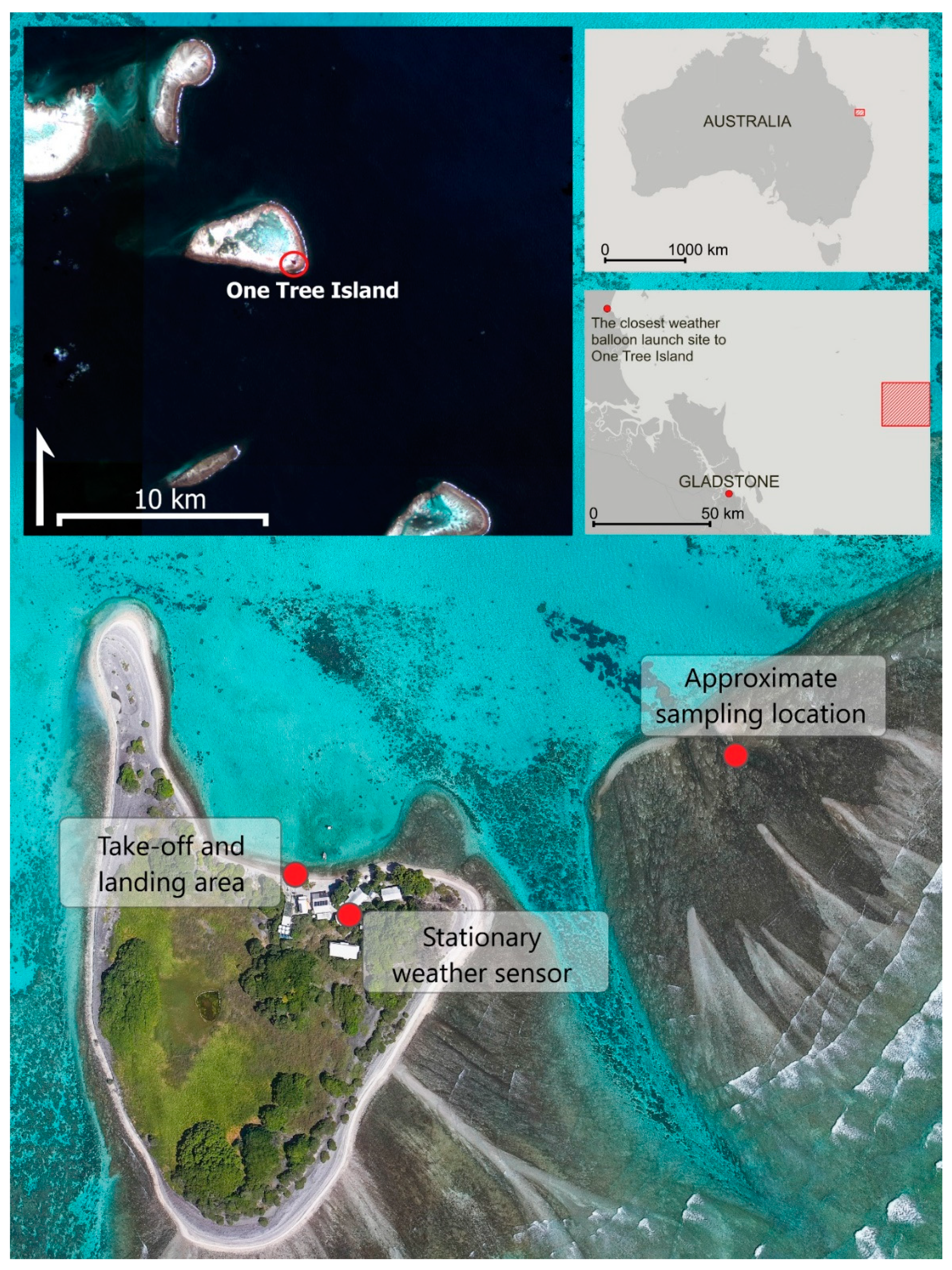
2.1. Sampling Methodology

Drones were utilised for profiling vertical atmospheric conditions up to 1500 m at One Tree Island Reef, located approximately 85 km offshore from the east coast of Australia (23.50833° S, 152.09167° E) in the southern section of the Great Barrier Reef (Figure 1). The prevailing weather conditions during the drone-based atmospheric profiles were fair, characterised by clear or partly cloudy skies. The data collection occurred between late February and early April 2023, with drone flights conducted beyond visual line of sight (BVLOS) and approved by the Australian Civil Aviation Safety Authority (CASA).
The vertical profiles were carried out using a DJI Matrice 300 (M300) quadcopter with duplicate InterMet Systems iMet-XQ2 UAV (iMet) atmospheric sensors. These sensors measure temperature, relative humidity, atmospheric pressure, and GNSS-derived position. The manufacturer calibrated both devices within the last 12 months before the campaign, specifying accuracies of ±0.3 °C for temperature, ±5% for relative humidity, ±1.5 hPa for air pressure, and ±12 m vertical accuracy for the GNSS sensor.
The iMet sensors were positioned on top of each other on the flat surface of the drone’s central main body. The primary reason for this setup was to reduce the risk of loosening parts during extended flight missions and to facilitate easy handling of sensors for data retrieval after the missions. Data are stored internally, and the device has to be connected via USB to a computer. The redundancy of two mounted sensors minimised the chance of potential data loss [38] and provided the opportunity to compare the sensors’ performance. The position of one sensor above the other gives insights into the influence of heat radiation from the drone batteries and other electric components.
Data from a reference weather sensor, the G. Lufft Mess- und Regeltechnik GmbH WS800-UMB Smart Weather Sensor (WS800), were compared to data from the iMet sensor. The WS800 weather sensor measured temperature, relative humidity, air pressure, wind direction, and wind speed. It was mounted on a mast 10 m above the ground, marking the highest point in its approximate surroundings. One Tree Island consists only of low-growing vegetation and single-story or split-level structures. The drone’s take-off area was positioned approximately 30 m horizontally from the WS800, and each start and end of the mission occurred at the same height as the sensor’s mounting point. The daily iMet profile with temperature measurements that better matched the WS800 values was selected for further analysis. Dewpoint temperature was calculated using the Magnus–Tetens formula [39].
Each vertical profile used a fully automated drone mission, although take-off and landing were performed manually to minimise the risk of bird strikes. A complete sampling day consisted of flights conducted at 0900, 1200, and 1500 (AEST), collecting data from 10 to 1500 m altitude. The ascent was performed with a vertical speed of 3 m/s, ensuring adequate ventilation for the iMet sensors [40]. The lower limit of 10 m was set due to safety considerations related to the drone’s proximity to the ocean, and the drone’s manufacturer set the upper limit. The start of the drone-based vertical profile also corresponded to the height of the WS800 weather sensor. During the vertical climb, the drone’s flight controller estimated the wind speed and direction using measurements from the inertial measurement unit and the response of the electronic speed controllers. The specific algorithm employed to calculate the wind vector estimate is implemented by the drone manufacturer DJI (Shenzhen, China) and remains undisclosed to the public. This approach should not be seen as a replacement for high-precision wind profile observations achieved through more sophisticated techniques [41]. Nevertheless, it can be considered valuable information, particularly in short-term field atmospheric research campaigns conducted in remote locations [42]. After excluding days with less than three completed flights, there were complete datasets for 24 days.

2.2. Analysis of Data
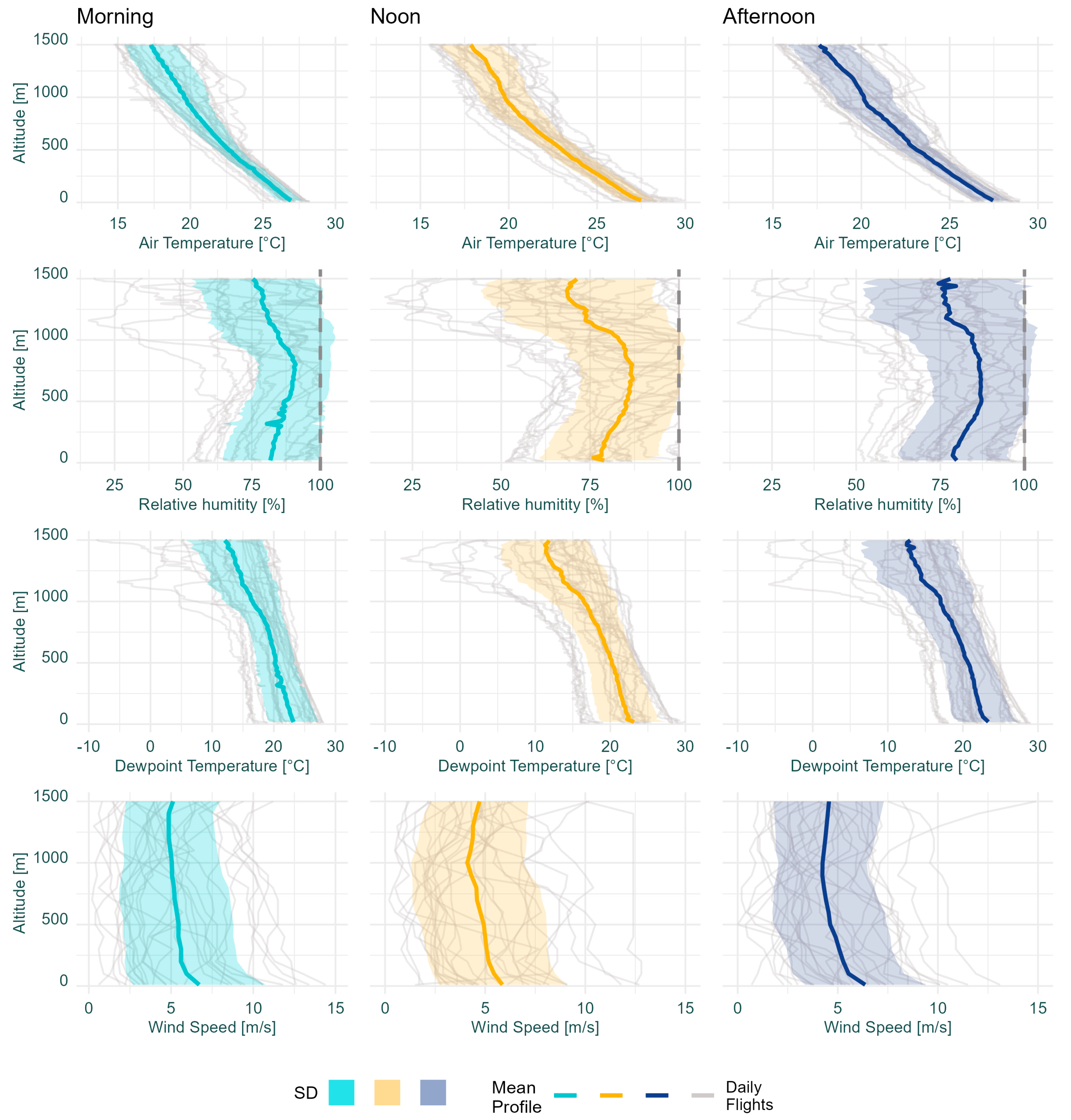
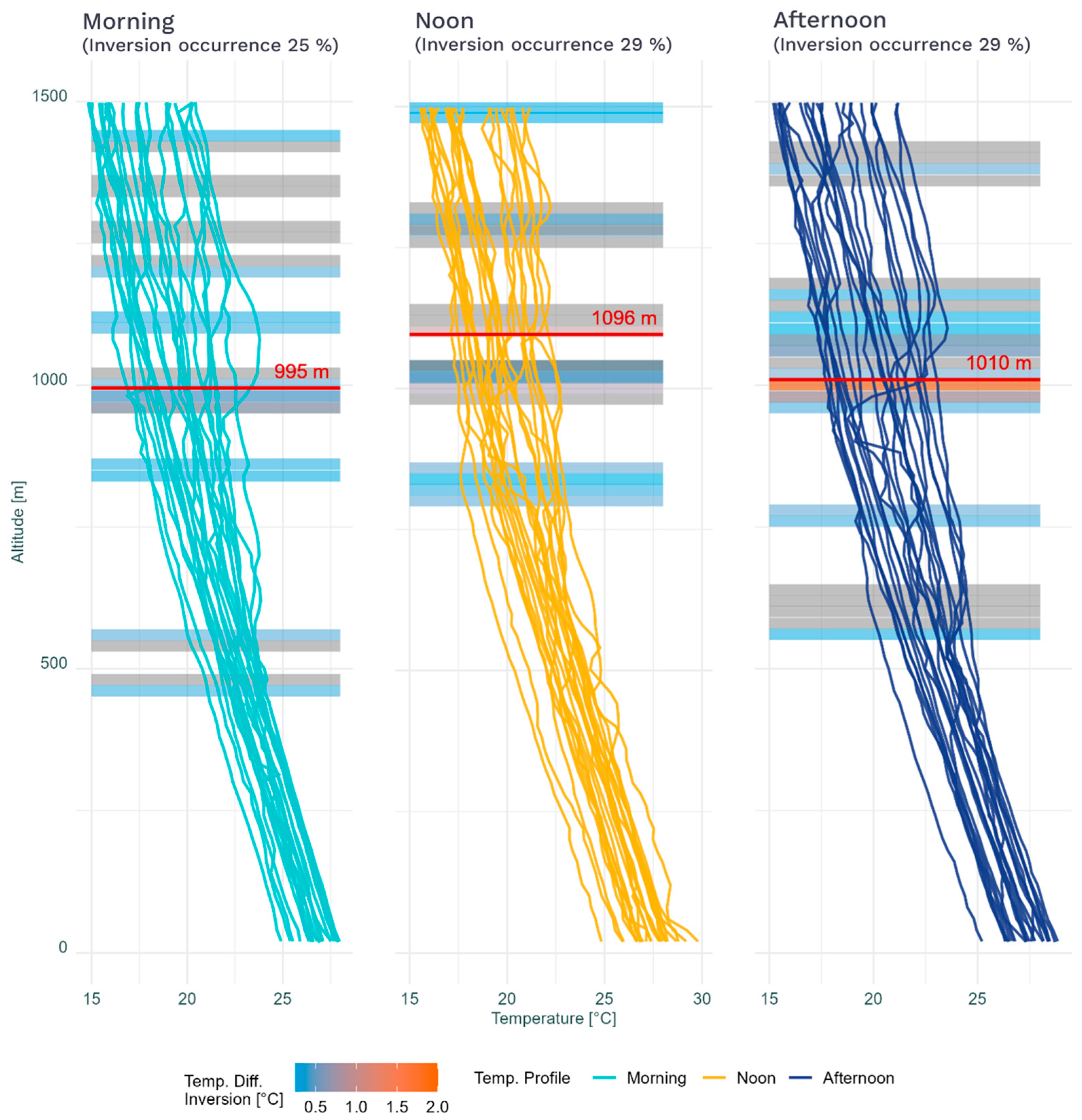
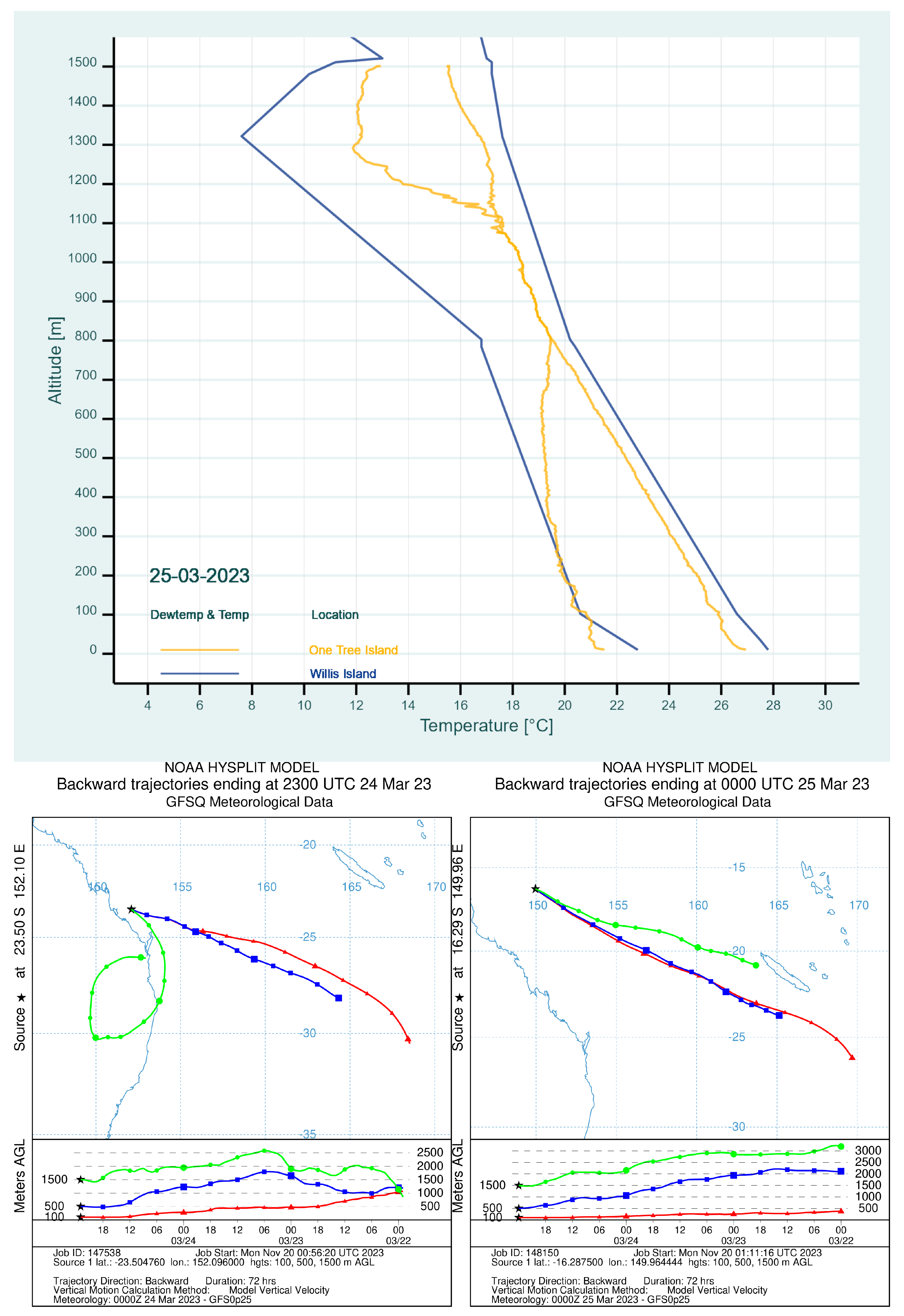
The data were collected by iMet sensors at 1 Hz. We organised the data into 20 m bins and calculated the average for each. To identify minor temperature inversions within the initial 1500 m of the atmosphere, we considered an inversion to have occurred if the temperature increased by at least 0.16 °C between a specific 20 m segment and the higher one following it, resulting in a temperature change rate of 0.8 °C/100 m. We also employed an additional processing step to remove rows marked as inversions when the temperature decreased again in the subsequent altitude bin. As a result, we retained only instances of inversions where the temperature increased over a vertical ascent of at least 40 m. These values are based on previous studies [43,44]. In the final stage, we calculated a weighted average inversion altitude for each vertical profile.
We used permutational analysis of variance (PERMANOVA) [45] to test the hypotheses that temperature, dewpoint temperature, atmospheric pressure, and wind speed varied significantly among sampling times. In these analyses, the factor time of day was considered orthogonally fixed with three levels (9 a.m., 12 noon, and 3 p.m.), and sampling day was treated as a random factor. Each vertical profile with its 75 altitude bins was used as an individual replicate in the PERMANOVA analyses, which were based on Euclidean distance and 9999 permutations. Following a significant main effect, pairwise post hoc tests were used to interrogate significant time of day effects. PERMANOVAs were carried out using the PRIMER 6 statistical software with the PERMANOVA+ add-on (PRIMER-e, Auckland, New Zealand).

3. Results

Over the 24 monitoring days in the Austral summer, the temperature at 10 m, 750 m, and 1500 m ranged from 25.1 to 29.2 °C, 18.3 to 24.2 °C, and 14.9 to 21.3 °C, respectively. Over the same heights, the dewpoint temperature ranged from 15.8 to 29.2 °C, 12.8 to 24.2 °C, and −8.6 to 19.0 °C. Generally, the average temperature and dewpoint temperature decreased with altitude by 35.6% and 47.3% at 1500 m compared to 10 m (Figure 2). The average air pressure also decreased by 15.7% between 10 and 1500 m. The air pressure was, however, much less variable than the temperature, ranging from 1006.5 to 1017.7 hPa, 924.0 to 935.8 hPa, and 943.7 to 957.9 hPa at 10 m, 750 m, and 1500 m, respectively (Figure 2). The relative humidity increased by 9.4% from 10 m to 750 m and decreased by 15.2% from 750 m to 1500 m. Over the whole altitude, the range of the relative humidity decreased by 7.2%, which results in an S-curve in the mean profiles (Figure 2). The average wind speed showed less variation with altitude compared to the other variables in the vertical profile (Figure 2). However, there was a pattern of slightly faster average wind speeds near the surface, followed by a decrease until 1000 m. From 1000 m, the average windspeed increased to 1500 m, where it was slightly less than that of the surface winds (Figure 2).
The vertical profile for temperature, dewpoint temperature, pressure, and wind speed all differed significantly among the days of sampling (Table 1). The vertical profiles for temperature at 9 a.m. differed significantly from those at 12 noon and 3 p.m., which did not differ from each other (Table 1, Figure 2). The mean (±SE) temperature at 9 a.m. was 21.4 ± 0.02 °C, which was 1.8% and 2.3% less than the temperatures at 12 noon and 3 p.m., respectively (Figure 2). Although PERMANOVA found significant differences in dewpoint temperatures and air pressures at different times of day, the post hoc tests were not powerful enough to find a clear pattern among sampling times (Table 1, Figure 2). Wind speed varied significantly among 9 a.m., 12 noon, and 3 p.m. The average (±SE) windspeeds at 9 a.m., 12 noon, and 3 p.m. were 4.8 ± 0.15 m/s, 4.7 ± 0.15 m/s, and 4.8 ± 0.14 m/s, respectively (Figure 2). Although the average windspeeds did not vary much among the times of sampling, the structure of the profiles varied enough to cause significant differences in the PERMANOVA analyses (Figure 2).
Each vertical profile’s temperature and relative humidity values at 10 m altitude were cross-referenced with measurements recorded by the reference weather station WS800 (Table 2). For the temperature, the iMet sensors consistently exhibited a warm bias compared to the WS800. Pre-mission measurements indicated the highest mean bias, surpassing 1 °C. During the mission, particularly at “Noon,” the top-mounted sensor peaked at +1.61 °C relative to the weather station measurement, while the body-mounted sensor reached 1.72 °C higher. Before take-off, the drone with mounted sensors underwent a 5–10 min pre-flight safety check on the landing pad, exposing the sensors to solar radiation with only aspiration due to the rotors and ambient wind. During the drone’s flight from the “Pre” to the “Start” position (approximately 300 m horizontal distance), the sensors were exposed to additional ventilation, resulting in a mean temperature difference drop of around −0.84 °C. Post-flight, the temperature bias between the WS800 and iMet measurements was at its minimum, with an overall mean difference of +0.30 °C and a standard deviation of 0.62 °C. The horizontal flight back to the “Post” position just before landing, with reduced sensor aspiration compared to the 3 m/s fast vertical ascent and descent, resulted in a mean temperature difference increase of 0.27 °C. The warm bias appeared more pronounced in the iMet sensor directly mounted to the drone’s body. Nevertheless, the lower temperature bias observed at the end of each mission, after being exposed to the 3 m/s strong aspiration, are very similar for both sensors regardless of their position on the drone (Table 2). For relative humidity, a much greater variability with no specific pattern of bias is present. The overall average of the mean difference comes to −5.53% relative to the WS800 with a standard deviation of 13.79%. This suggests potential limitations in the iMet relative humidity sensor’s performance (Table 2).
In the Austral summer around One Tree Island, microscale temperature inversion layers were observed in 27% of the measured profiles (Figure 3). Microscale temperature inversions were most frequent at around 1000 m throughout the daily cycle, peaking in height around noon. Temperature inversions also occurred in the morning (i.e., 9 a.m.) at around 500 m as the well-mixed boundary layer developed. Around noon, no inversions are observed below 750 m. In the afternoon, the layer around 1000 m became more distinct and compact. New inversion layers sometimes appeared between 500 and 700 m around 3 p.m.

4. Discussion

Consumer drones combined with economical meteorological sensors provide a practical solution for vertically measuring temperature, pressure, relative humidity, wind speed, and direction from altitudes of 10 m up to 1500 m. Our drone-based vertical profiles showed clear patterns of difference in temperature and dewpoint temperature at different sampling times near One Tree Island. The drone monitoring also revealed the presence of microscale temperature inversions, primarily around 1000 m, on 27% of the observed days. These inversions displayed the variations in height and frequency associated with the time of day. A real benefit of the drone-based vertical profiles of the atmosphere is that they can be undertaken multiple times per day, capturing diurnal fluctuations in atmospheric characteristics and temperature inversions. In scenarios when only one profile per day is logistically possible, our results suggest that noon as a take-off time might be the most useful time. The average atmospheric conditions around noon were not always significantly different from 9 a.m. and 3 p.m. Furthermore, the vertical profile of meteorological variables around noon captured temperature inversions that could influence local weather conditions and coincided with the peak of convective mixing [12].
We demonstrated that drone-based sampling of three vertical profiles per day, spaced 3 h apart, can be achieved safely and reliably over an extended period. Unlike the lower atmosphere over land, which experiences significant temperature fluctuations due to radiative heat, the depth of the atmospheric boundary layer over the ocean changes slowly due to substantial mixing and water’s high heat capacity, resulting in minimal temperature variation over a day [1,12,46]. This difference in the behaviour of the atmospheric boundary layer over land and the ocean makes radiosonde soundings from the Australian mainland unsuitable for characterising the meteorological properties over One Tree Island. Willis Island, the closest ocean-sounding site, is approximately 835 km from One Tree Island and cannot provide the fine-scale atmospheric profiles of the local meteorological needed to initialise and validate numerical simulations for investigating cloud responses to aerosol injections [47,48], even when the relevant air parcel trajectories are modelled (Hybrid Single-Particle Lagrangian Integrated Trajectory model (HYSPLIT) [49]) to reach the sampling areas from the same direction (Figure 4). Therefore, localised atmospheric measurements are important for enhancing modelling efforts in remote areas to resolve the local diurnal transition periods, and we demonstrate that drones are forms of useful technology to help obtain these measurements. For future campaigns, it might be sensible to aim for at least two samplings per given day. One sampling at noon provides information about the peak of the mixing layer height. Additional profiles taken in the morning or afternoon can provide more detailed information about the transition phases. An hourly or sub-hourly observation cycle of variables like temperature, humidity, and wind may be desirable for improving high-frequency, high-impact weather prediction in operational scenarios, such as thunderstorms and fog [36]. It should be noted, however, it took around half an hour to complete each vertical profile, including pre-flight checks and post-flight inspections. In terms of optimising drone-based vertical profiles for highly detailed characterisations of the lower atmosphere, the 3D Mesonet proposes vertical profiling using multirotor drones up to an altitude of 2000 m every 90 min [37]. While valuable, this intense sampling would require a drone that was capable of flying 500 m higher than the M300 drone we used in our study, as well as a team of pilots, technicians, and researchers.
The repeated sampling of high vertical resolution temperature measurements up to 1500 m allowed us to capture diurnal fluctuations in the formation of temperature inversions, providing insights into the dispersal behaviour of aerosols such as sea spray aerosols, volatile organic compounds, and pollutants [50]. Temperature inversions can suppress the vertical mixing of the atmosphere, creating stable layers that inhibit the upward movement of aerosols. An inversion layer is characterised by a portion of the atmosphere where temperature rises as altitude increases as it deviates from the normal condition where air temperature decreases with altitude [51]. There are multiple methods for detecting temperature inversions [46], but we focused on the diurnal patterns of these weather phenomena rather than a more detailed analysis of their structure. Monitoring changes in temperature inversions throughout the day provides insight into their influence on atmospheric dynamics and understanding aerosol dispersion. To gain more complex insights, additional aerosol measurement instruments can be considered [52,53]. While the work undertaken at One Tree Island offered valuable insights into temperature inversions, the observations were constrained to fair-weather conditions, with clear or partly cloudy skies. In the present study, drone-based vertical profiles were not collected during strong winds, rain squalls, or extreme weather events. Therefore, our dataset only represents ‘non-extreme’ meteorological conditions over the southern Great Barrier Reef.
Accurately associating location (altitude, latitude, and longitude) with atmospheric characteristics improves the overall quality of meteorological data. Compared to weather balloon soundings, drone-based atmospheric profiles remained fixed in latitude and longitude throughout the entire duration of the data collection. The integration of the M300 drone’s altitude measurements into the dataset significantly enhanced height precision compared to the iMet sensor’s GNSS system [54] and made the calculation process of a pressure altitude unnecessary. The drone also estimated wind speed and direction based on the power needed to maintain its flight path. Overall, the drone’s performance in the present study adds to the growing evidence of the value of drones for in situ meteorological data collection [36,55,56]. Using drones to improve weather forecasts also has substantial public support [57].
The marine boundary layer can be defined as the lowest part of the troposphere that is directly influenced by the Earth’s surface, which responds to surface forcing within one hour or less [12]. Coral reefs influence the surface roughness, temperature, and humidity of the ocean, sometimes leading to a connection of the ocean with the overlying atmosphere, in the form of a convective internal atmospheric boundary layer within the marine boundary layer [1,58,59]. The convective internal atmospheric boundary layer is usually characterised by an interpretation of wind speed, vertical profiles of virtual potential temperature, and mixing ratio [59,60]. The drone-based vertical profiles measured changes in temperature, relative humidity, atmospheric pressure, and wind parameters multiple times per day. Such high-resolution datasets could be applied to providing further insight into the potential coupling of coral reefs with the overlying atmosphere [59,60].
Different operational measurements can be used to estimate the marine boundary layer depth [3]. One approach involves using temperature and humidity profiles to determine the boundary layer’s height [61,62,63]. This method is ideally suited for well-defined inversions in potential temperature and corresponding decreases in specific humidity [1,12]. However, in real-world boundary layer conditions, the stability can fluctuate between stable and unstable, introducing uncertainties [3,64]. An alternative approach for verifying estimated boundary layer heights from meteorological soundings is to compare these estimates with measurements obtained from backscatter light detection and ranging (LiDAR) systems [65,66,67]. The collection of vertical atmospheric profiles holds the potential for future comparisons of retrieved boundary layer heights with those estimated from LiDAR systems, thereby validating the methods used [36,52].
Daily drone-based sampling for vertical atmospheric profiles over One Tree Island required a specially trained CASA-certified BVLOS pilot and a qualified observer, even though the sampling flight was entirely automated. It would be worth exploring the potential of the “drone in a box” concept to increase the cost-effectiveness of drone-based profiles. This concept involves a fully autonomous drone housed in a weatherproof box and charging station [68,69]. The box unlocks at the beginning of a mission, allowing the drone to launch and carry out its mission autonomously. Alternatively, operators could remotely operate it using satellite or mobile internet communication [69]. Automation within drone technology has the potential to enhance cost-effectiveness by reducing the reliance on trained personnel. In the case of One Tree Island, existing on-site staff, such as the research station caretaker, could potentially be trained to operate the “drone in a box”. Additional risk mitigation and monitoring of the flight may be needed to address the potential bird hazard mentioned earlier. Nonetheless, a fully autonomous drone mission flying into airspace accessible to crewed aircraft would also require significant risk mitigations to comply with airspace regulations in many countries including at our Great Barrier Reef site. Exploring this direction could offer an affordable alternative for research purposes compared to more expensive specialised systems and crew [70].

5. Conclusions

Despite the challenges posed by regulatory and logistical constraints, consumer drones equipped with lightweight sensors were an effective solution for collecting vertical profiles of meteorological conditions in the remote oceanic location of One Tree Island, Australia. The drones successfully measured vertical profiles of atmospheric pressure, temperature, humidity, and wind over altitudes ranging from 10 m to 1500 m, providing valuable insights into diurnal variations and temperature inversions within the atmospheric boundary layer. The data collected offer opportunities for further research, particularly in exploring the interaction between coral reefs and the atmosphere, a daily assessment of boundary layer stratification, and its influence on heat and moisture exchange, cloud formation, and aerosol behaviour. Future investigations into the use of drones for atmospheric profiling should be pursued. Incorporating additional instrumentation, such as aerosol counters, cloud droplet probes, and cameras, could provide more detailed insights into existing cloud layers and the characteristics of the boundary layer. Drone technology can make meteorological data collection more accessible, affordable, and available for remote locations.

Author Contributions

Conceptualisation, C.E., B.P.K. and D.P.H.; writing—original draft, C.E.; writing—review and editing, C.E., B.P.K., K.I.M. and D.P.H.; visualisation, C.E.; investigation, C.E., B.P.K. and K.I.M.; data curation, C.E. and K.I.M.; formal analysis, C.E.; project administration, B.P.K. and D.P.H.; funding acquisition, D.P.H. and B.P.K. All authors have read and agreed to the published version of the manuscript.

Funding

This work was undertaken for the Reef Restoration and Adaptation Program (Cooling and shading sub-program), funded by the partnership between the Australian Government’s Reef Trust and the Great Barrier Reef Foundation.

Data Availability Statement

The raw data supporting the conclusions of this article will bemade available by the authors on request.

Acknowledgments

We extend our deepest respect and recognition to the Gooreng Gooreng, Gurang, Bailai, and Taribelang Bunda peoples, the traditional custodians of the area around One Tree Island as First Nations Peoples holding the hopes, dreams, traditions, and cultures of the Great Barrier Reef Sea Country. We thank Robyn Schofield and Robert Ryan of The University of Melbourne for providing meteorological data from the ground-based weather station. We are also grateful to Mark Goolmeer and Stephen Childs for their help with fieldwork.

Conflicts of Interest

The authors declare no conflict of interest.

References

  1. Garratt, J.R. The atmospheric boundary layer. Earth-Sci. Rev. 1994, 37, 89–134. [Google Scholar] [CrossRef]
  2. Wood, R. Stratocumulus clouds. Mon. Weather Rev. 2012, 140, 2373–2423. [Google Scholar] [CrossRef]
  3. Seibert, P.; Beyrich, F.; Gryning, S.-E.; Joffre, S.; Rasmussen, A.; Tercier, P. Review and intercomparison of operational methods for the determination of the mixing height. Atmos. Environ. 2000, 34, 1001–1027. [Google Scholar] [CrossRef]
  4. Bureau of Meteorology & CSIRO. State of the Climate 2022; Bureau of Meteorology & CSIRO: Canberra, Australia, 2022. [Google Scholar]
  5. Australian Government, The Treasury. 2023 Intergenerational Report; Australian Government, The Treasury: Sydney, Australia, 2023. [Google Scholar]
  6. Guo, S.; Li, J.; Yao, W.; Zhan, Y.; Li, Y.; Shi, Y. Distribution characteristics on droplet deposition of wind field vortex formed by multi-rotor UAV. PLoS ONE 2019, 14, e0220024. [Google Scholar] [CrossRef] [PubMed]
  7. Deloitte. The Turning Point a Global Summary; Deloitte Development LLC: London, UK, 2022. [Google Scholar]
  8. World Meteorological Organization. The Gaps in the Global Basic Observing Network (GBON); WMO: Geneva, Switzerland, 2020. [Google Scholar]
  9. Wang, B.; Zou, X.; Zhu, J. Data assimilation and its applications. Proc. Natl. Acad. Sci. USA 2000, 97, 11143–11144. [Google Scholar] [CrossRef] [PubMed]
  10. Illingworth, A.J.; Cimini, D.; Haefele, A.; Haeffelin, M.; Hervo, M.; Kotthaus, S.; Löhnert, U.; Martinet, P.; Mattis, I.; O’Connor, E.J.; et al. How Can Existing Ground-Based Profiling Instruments Improve European Weather Forecasts? Bull. Am. Meteorol. Soc. 2019, 100, 605–619. [Google Scholar] [CrossRef]
  11. Altstädter, B.; Platis, A.; Wehner, B.; Scholtz, A.; Wildmann, N.; Hermann, M.; Käthner, R.; Baars, H.; Bange, J.; Lampert, A. ALADINA—An unmanned research aircraft for observing vertical and horizontal distributions of ultrafine particles within the atmospheric boundary layer. Atmos. Meas. Tech. 2015, 8, 1627–1639. [Google Scholar] [CrossRef]
  12. Stull, R.B. An Introduction to Boundary Layer Meteorology; Springer Science & Business Media: New York, NY, USA, 1988; Volume 13. [Google Scholar]
  13. Porté-Agel, F.; Bastankhah, M.; Shamsoddin, S. Wind-turbine and wind-farm flows: A review. Bound.-Layer Meteorol. 2020, 174, 1–59. [Google Scholar] [CrossRef]
  14. Li, L.; Gao, L.; Liu, Y.; Cui, Y.; Wang, B. Field measurements of atmospheric boundary layer and the impact of its daily variation on wind turbine wakes. In Proceedings of the 5th IET International Conference on Renewable Power Generation (RPG 2016), London, UK, 21–23 September 2016. [Google Scholar]
  15. Kumar, A.; Ambika, R. Drone Integrated Weather Sensors for Agriculture Purpose. Int. J. Electr. Eng. Technol. 2020, 11, 83–90. [Google Scholar]
  16. Kotthaus, S.; Bravo-Aranda, J.A.; Collaud Coen, M.; Guerrero-Rascado, J.L.; Costa, M.J.; Cimini, D.; O’Connor, E.J.; Hervo, M.; Alados-Arboledas, L.; Jiménez-Portaz, M.; et al. Atmospheric boundary layer height from ground-based remote sensing: A review of capabilities and limitations. Atmos. Meas. Tech. 2023, 16, 433–479. [Google Scholar] [CrossRef]
  17. Bouttier, F.; Kelly, G. Observing-system experiments in the ECMWF 4D-Var data assimilation system. Q. J. R. Meteorol. Soc. 2001, 127, 1469–1488. [Google Scholar]
  18. Eyre, J.R.; English, S.J.; Forsythe, M. Assimilation of satellite data in numerical weather prediction. Part I: The early years. Q. J. R. Meteorol. Soc. 2020, 146, 49–68. [Google Scholar] [CrossRef]
  19. Eyre, J.; Bell, W.; Cotton, J.; English, S.; Forsythe, M.; Healy, S.; Pavelin, E. Assimilation of satellite data in numerical weather prediction. Part II: Recent years. Q. J. R. Meteorol. Soc. 2022, 148, 521–556. [Google Scholar] [CrossRef]
  20. Greene, B.R.; Segales, A.R.; Waugh, S.; Duthoit, S.; Chilson, P.B. Considerations for temperature sensor placement on rotary-wing unmanned aircraft systems. Atmos. Meas. Tech. 2018, 11, 5519–5530. [Google Scholar] [CrossRef]
  21. Lee, T.R.; Buban, M.; Dumas, E.; Baker, C.B. On the Use of Rotary-Wing Aircraft to Sample Near-Surface Thermodynamic Fields: Results from Recent Field Campaigns. Sensors 2019, 19, 10. [Google Scholar] [CrossRef]
  22. DuBois, J.L. Invention and Development of the Radiosonde with a Catalog of Upper-Atmospheric Telemetering Probes in the National Museum of American History, Smithsonian Institution. Smithson. Stud. Hist. Technol. 2002, 53, 1–78. [Google Scholar] [CrossRef]
  23. Jones, N. High-altitude balloons: What’s up there and why. Nature 2023, 614, 606. [Google Scholar] [CrossRef]
  24. Ingleby, B.; Edwards, D. Changes to radiosonde reports and their processing for numerical weather prediction. Atmos. Sci. Lett. 2015, 16, 44–49. [Google Scholar] [CrossRef]
  25. Bureau of Meteorology. Balloon-Based Weather Observations; Australian Government, Bureau of Meteorology: Canberra, Australia, 2018. [Google Scholar]
  26. Douglas, M. Adaptive sounding arrays for tropical regions. In Proceedings of the Extended Abstracts, 29th Conf. on Hurricanes and Tropical Meteorology, Tucson, AZ, USA, 10–14 May 2010; pp. 12B–17B. [Google Scholar]
  27. Villa, T.F.; Gonzalez, F.; Miljievic, B.; Ristovski, Z.D.; Morawska, L. An overview of small unmanned aerial vehicles for air quality measurements: Present applications and future prospectives. Sensors 2016, 16, 1072. [Google Scholar] [CrossRef]
  28. Hock, T.F.; Franklin, J.L. The NCAR GPS Dropwindsonde. Bull. Am. Meteorol. Soc. 1999, 80, 407–420. [Google Scholar] [CrossRef]
  29. O’Shea, O.R.; Hamann, M.; Smith, W.; Taylor, H. Predictable pollution: An assessment of weather balloons and associated impacts on the marine environment—An example for the Great Barrier Reef, Australia. Mar. Pollut. Bull. 2014, 79, 61–68. [Google Scholar] [CrossRef] [PubMed]
  30. Daniel, J.T.; Costidis, A.M.; Barco, S.G. Fatal entanglements of sea turtles caused by widely deployed weather instruments. Mar. Pollut. Bull. 2023, 193, 115108. [Google Scholar] [CrossRef] [PubMed]
  31. Valencia, M.A.C.; Cruz, F.R.G.; Balakit, R.B. LoRa Transmission System for Weather Balloons. In Proceedings of the 2019 IEEE 11th International Conference on Humanoid, Nanotechnology, Information Technology, Communication and Control, Environment, and Management (HNICEM), Laoag, Philippines, 29 November–1 December 2019; pp. 1–5. [Google Scholar]
  32. Greatwood, C.; Richardson, T.S.; Freer, J.; Thomas, R.M.; MacKenzie, A.R.; Brownlow, R.; Lowry, D.; Fisher, R.E.; Nisbet, E.G. Atmospheric Sampling on Ascension Island Using Multirotor UAVs. Sensors 2017, 17, 1189. [Google Scholar] [CrossRef] [PubMed]
  33. Greene, B.R.; Segales, A.R.; Bell, T.M.; Pillar-Little, E.A.; Chilson, P.B. Environmental and sensor integration influences on temperature measurements by rotary-wing unmanned aircraft systems. Sensors 2019, 19, 1470. [Google Scholar] [CrossRef] [PubMed]
  34. Islam, A.; Houston, A.L.; Shankar, A.; Detweiler, C. Design and evaluation of sensor housing for boundary layer profiling using multirotors. Sensors 2019, 19, 2481. [Google Scholar] [CrossRef] [PubMed]
  35. World Meteorological Organization. Global Demonstration Campaign for Evaluating the Use of Uncrewed Aircraft Systems in Operational Meteorology: White Paper (WMO-No. 1318); WMO: Geneva, Switzerland, 2023. [Google Scholar]
  36. Leuenberger, D.; Haefele, A.; Omanovic, N.; Fengler, M.; Martucci, G.; Calpini, B.; Fuhrer, O.; Rossa, A. Improving high-impact numerical weather prediction with lidar and drone observations. Bull. Am. Meteorol. Soc. 2020, 101, E1036–E1051. [Google Scholar] [CrossRef]
  37. Chilson, P.B.; Bell, T.M.; Brewster, K.A.; Britto Hupsel de Azevedo, G.; Carr, F.H.; Carson, K.; Doyle, W.; Fiebrich, C.A.; Greene, B.R.; Grimsley, J.L. Moving towards a network of autonomous UAS atmospheric profiling stations for observations in the Earth’s lower atmosphere: The 3D mesonet concept. Sensors 2019, 19, 2720. [Google Scholar] [CrossRef]
  38. Kimball, S.K.; Montalvo, C.J.; Mulekar, M.S. Assessing iMet-XQ performance and optimal placement on a small off-the-shelf, rotary-wing UAV, as a function of atmospheric conditions. Atmosphere 2020, 11, 660. [Google Scholar] [CrossRef]
  39. Alduchov, O.A.; Eskridge, R.E. Improved Magnus Form Approximation of Saturation Vapor Pressure. J. Appl. Meteorol. Climatol. 1996, 35, 601–609. [Google Scholar] [CrossRef]
  40. Kimball, S.K.; Montalvo, C.J.; Mulekar, M.S. Evaluating temperature measurements of the iMET-XQ, in the field, under varying atmospheric conditions. Atmosphere 2020, 11, 335. [Google Scholar] [CrossRef]
  41. Wang, J.-Y.; Luo, B.; Zeng, M.; Meng, Q.-H. A Wind Estimation Method with an Unmanned Rotorcraft for Environmental Monitoring Tasks. Sensors 2018, 18, 4504. [Google Scholar] [CrossRef] [PubMed]
  42. Varentsov, M.; Stepanenko, V.; Repina, I.; Artamonov, A.; Bogomolov, V.; Kuksova, N.; Marchuk, E.; Pashkin, A.; Varentsov, A. Balloons and quadcopters: Intercomparison of two low-cost wind profiling methods. Atmosphere 2021, 12, 380. [Google Scholar] [CrossRef]
  43. Yang, Y.; Ni, C.; Jiang, M.; Chen, Q. Effects of aerosols on the atmospheric boundary layer temperature inversion over the Sichuan Basin, China. Atmos. Environ. 2021, 262, 118647. [Google Scholar] [CrossRef]
  44. Fochesatto, G.J. Methodology for determining multilayered temperature inversions. Atmos. Meas. Tech. 2015, 8, 2051–2060. [Google Scholar] [CrossRef]
  45. Anderson, M.J. Permutational Multivariate Analysis of Variance (PERMANOVA). In Wiley StatsRef: Statistics Reference Online; John Wiley & Sons, Ltd.: Hoboken, NJ, USA, 2017; pp. 1–15. [Google Scholar]
  46. Seidel, D.J.; Zhang, Y.; Beljaars, A.; Golaz, J.C.; Jacobson, A.R.; Medeiros, B. Climatology of the planetary boundary layer over the continental United States and Europe. J. Geophys. Res. Atmos. 2012, 117, D17106. [Google Scholar] [CrossRef]
  47. Hoffmann, F.; Feingold, G. Cloud Microphysical Implications for Marine Cloud Brightening: The Importance of the Seeded Particle Size Distribution. J. Atmos. Sci. 2021, 78, 3247–3262. [Google Scholar] [CrossRef]
  48. Sullivan, P.P.; McWilliams, J.C.; Moeng, C.-H. A subgrid-scale model for large-eddy simulation of planetary boundary-layer flows. Bound.-Layer Meteorol. 1994, 71, 247–276. [Google Scholar] [CrossRef]
  49. Stein, A.F.; Draxler, R.R.; Rolph, G.D.; Stunder, B.J.B.; Cohen, M.D.; Ngan, F. NOAA’s HYSPLIT Atmospheric Transport and Dispersion Modeling System. Bull. Am. Meteorol. Soc. 2015, 96, 2059–2077. [Google Scholar] [CrossRef]
  50. Lewis, E.R.; Schwartz, S.E. Sea Salt Aerosol Production: Mechanisms, Methods, Measurements, and Models; American Geophysical Union: Washington, DC, USA, 2004; Volume 152. [Google Scholar]
  51. Bilello, M.A. Survey of Arctic and Subarctic Temperature Inversions; Cold Regions Research and Engineering Laboratory: Handover, NH, USA, 1966. [Google Scholar]
  52. Inoue, J.; Sato, K. Challenges in Detecting Clouds in Polar Regions Using a Drone with Onboard Low-Cost Particle Counter. Atmos. Environ. 2023, 314, 120085. [Google Scholar] [CrossRef]
  53. Liu, Z.; Osborne, M.; Anderson, K.; Shutler, J.D.; Wilson, A.; Langridge, J.; Yim, S.H.L.; Coe, H.; Babu, S.; Satheesh, S.K.; et al. Characterizing the performance of a POPS miniaturized optical particle counter when operated on a quadcopter drone. Atmos. Meas. Tech. 2021, 14, 6101–6118. [Google Scholar] [CrossRef]
  54. Islam, A.; Shankar, A.; Houston, A.; Detweiler, C. University of Nebraska unmanned aerial system (UAS) profiling during the LAPSE-RATE field campaign. Earth Syst. Sci. Data 2021, 13, 2457–2470. [Google Scholar] [CrossRef]
  55. Pinto, J.O.; Jensen, A.A.; Steiner, M.; O’Sullivan, D.; Taylor, S.; Elston, J.; Baker, C.B.; Hotz, D.; Marshall, C.; Jacob, J. The status and future of small uncrewed aircraft systems (UAS) in operational meteorology. Bull. Am. Meteorol. Soc. 2021, 102, E2121–E2136. [Google Scholar]
  56. Inoue, J.; Sato, K. Toward sustainable meteorological profiling in polar regions: Case studies using an inexpensive UAS on measuring lower boundary layers with quality of radiosondes. Environ. Res. 2022, 205, 112468. [Google Scholar] [CrossRef] [PubMed]
  57. Walther, J.; PytlikZillig, L.; Detweiler, C.; Houston, A. How people make sense of drones used for atmospheric science (and other purposes): Hopes, concerns, and recommendations. J. Unmanned Veh. Syst. 2019, 7, 219–234. [Google Scholar] [CrossRef]
  58. Garratt, J.R. The internal boundary layer—A review. Bound.-Layer Meteorol. 1990, 50, 171–203. [Google Scholar] [CrossRef]
  59. McGowan, H.; Lensky, N.G.; Abir, S.; Saunders, M. Coral Reef Coupling to the Atmospheric Boundary Layer Through Exchanges of Heat, Moisture, and Momentum: Case Studies From Tropical and Desert Fringing Coral Reefs. Front. Mar. Sci. 2022, 9, 900679. [Google Scholar] [CrossRef]
  60. MacKellar, M.C.; McGowan, H.A.; Phinn, S.R. An observational heat budget analysis of a coral reef, Heron Reef, Great Barrier Reef, Australia. J. Geophys. Res. Atmos. 2013, 118, 2547–2559. [Google Scholar] [CrossRef]
  61. Guo, J.; Miao, Y.; Zhang, Y.; Liu, H.; Li, Z.; Zhang, W.; He, J.; Lou, M.; Yan, Y.; Bian, L.; et al. The climatology of planetary boundary layer height in China derived from radiosonde and reanalysis data. Atmos. Chem. Phys. 2016, 16, 13309–13319. [Google Scholar] [CrossRef]
  62. Wang, X.; Wang, K. Homogenized variability of radiosonde-derived atmospheric boundary layer height over the global land surface from 1973 to 2014. J. Clim. 2016, 29, 6893–6908. [Google Scholar] [CrossRef]
  63. Zhang, H.; Zhang, X.; Li, Q.; Cai, X.; Fan, S.; Song, Y.; Hu, F.; Che, H.; Quan, J.; Kang, L. Research progress on estimation of the atmospheric boundary layer height. J. Meteorol. Res. 2020, 34, 482–498. [Google Scholar] [CrossRef]
  64. Johansson, C.; Bergström, H. An Auxiliary Tool to Determine the Height of the Boundary Layer. Bound.-Layer Meteorol. 2005, 115, 423–432. [Google Scholar] [CrossRef]
  65. Hennemuth, B.; Lammert, A. Determination of the Atmospheric Boundary Layer Height from Radiosonde and Lidar Backscatter. Bound. -Layer Meteorol. 2006, 120, 181–200. [Google Scholar] [CrossRef]
  66. Lammert, A.; Bösenberg, J. Determination of the convective boundary-layer height with laser remote sensing. Bound.-Layer Meteorol. 2006, 119, 159–170. [Google Scholar] [CrossRef]
  67. Wang, Y.-C.; Wang, S.-H.; Lewis, J.R.; Chang, S.-C.; Griffith, S.M. Determining planetary boundary layer height by micro-pulse lidar with validation by UAV measurements. Aerosol Air Qual. Res. 2021, 21, 200336. [Google Scholar] [CrossRef]
  68. Galimov, M.; Fedorenko, R.; Klimchik, A. UAV Positioning Mechanisms in Landing Stations: Classification and Engineering Design Review. Sensors 2020, 20, 3648. [Google Scholar] [CrossRef]
  69. Langåker, H.-A.; Kjerkreit, H.; Syversen, C.L.; Moore, R.J.; Holhjem, Ø.H.; Jensen, I.; Morrison, A.; Transeth, A.A.; Kvien, O.; Berg, G.; et al. An autonomous drone-based system for inspection of electrical substations. Int. J. Adv. Robot. Syst. 2021, 18, 17298814211002973. [Google Scholar] [CrossRef]
  70. Hervo, M.; Romanens, G.; Martucci, G.; Weusthoff, T.; Haefele, A. Evaluation of an Automatic Meteorological Drone Based on a 6-Month Measurement Campaign. Atmosphere 2023, 14, 1382. [Google Scholar] [CrossRef]
Figure 1. One Tree Island Reef is situated in the southern region of the Great Barrier Reef (Source: Esri, ESA, and M. Goolmeer). The nearest field station, where the Australian Bureau of Meteorology routinely launches weather balloons with atmospheric sensors, is located near Yeppoon, approximately 150 km from One Tree Island Reef. Willis Island, the closest ocean-sounding site, is significantly more distant at 835 km.The horizontal distance between the stationary weather sensor and the sampling location is around 300 m.
Drones 07 00695 g001
Figure 2. Vertical profiles of air temperature, relative humidity, dewpoint temperature, and wind speed were averaged at 9 a.m., 12 noon, and 3 p.m., along with their respective standard deviations. The grey line graphs represent all the recorded profiles, and variability was evaluated within each 20 m altitude bin. The dashed line in the relative humidity plots mark the point of full saturation of the air.
Drones 07 00695 g002
Figure 3. Microscale temperature inversions are characterised by a temperature rise of ≥0.16 °C between adjacent 20 m altitude bins, progressing upward. A minimum of two consecutive layers of increasing temperature must be observed to be considered an inversion and further analysed. The weighted mean altitudes are computed based on the magnitude of temperature increases.
Drones 07 00695 g003
Figure 4. This figure compares the sampled meteorological profile on the morning of 25 March 2023 (2300 UTC on 24 March 2023), with the corresponding sounding from the Willis Island radiosonde on 25 March 2023, at 0000 UTC. The distance between the two sites is approximately 835 km. Each sounding displays the dewpoint temperature and temperature profiles from each site. The bottom of the plot presents the HYSPLIT backward trajectory, calculated 72 h back from the sampling time. The meteorological data comes from the 0.25-degree Global Forecasting System. On the left is One Tree Island, and on the right is Willis Island. The trajectories for both sites are estimated at three arrival altitudes (100 m, 500 m, and 1500 m). For this particular day, the air parcels are assumed to have followed quite a similar pathway for both sites.
Drones 07 00695 g004
Table 1. Overview of PERMANOVA results and post hoc tests for air temperature, dewpoint temperature, air pressure, and wind speed, with time and day as predictor variables. For the post-hoc tests, 9 = 9 a.m., 12 = 12 noon and 3 = 3 p.m., ≠ is p < 0.05 and = is p > 0.05.
.Air
Temperature
Dewpoint
Temperature
Air
Pressure
Wind
Speed
dfP-FPP-FPP-FPP-FP
Time26.73<0.011.790.1058.86<0.010.350.90
Day2317.13<0.0120.24<0.0146.78<0.0112.28<0.01
Post hoc
tests
9 ≠ 12 = 3 9 = 12 ≠ 3 9 = 12 = 3 9 ≠ 12 ≠ 3
Table 2. The means (°C) and standard deviations (°C) of temperature differences between the drone-based sensor and WS800 measurements (TDrone—TWS800), along with the means (%) and standard deviations (%) of relative humidity differences between the drone-based sensor and WS800 measurements (RHDrone—RHWS800), are categorised by flight time and temporal points of the flight mission and mounting position on the drone. Flight time categories include 9 a.m. (“Morning”), 12 (“Noon”), and 3 p.m. (“Afternoon”). Temporal points in the flight mission consist of “Pre” (just after take-off with the drone at an altitude above 10 m, around 30 m horizontal distance to the WS800), “Start” (beginning of the mission at 10 m altitude after a few minutes of sensor aspiration, around 300 m horizontal flight distance), “End” (mission conclusion at 10 m altitude with approximately 300 m horizontal distance to the WS800 sensor), and “Post” (just before landing at 10 m altitude, around 30 m horizontal distance to the WS800 weather station). “Top” marks the sensor mounted on top, and “Body” denotes the sensor positioned directly on the housing of the drone. The sample size for each flight time category was 24 per sensor and temporal point. The mean time difference between the compared measurements of the iMet and the WS800 was 7.2 s.
Difference Temperature
(TDrone—TWS800)
MorningNoonAfternoon
PositionStatusMean
(°C)
SD
(°C)
Mean
(°C)
SD
(°C)
Mean
(°C)
SD
(°C)
TopPre1.100.691.610.881.190.69
BodyPre1.220.741.721.101.030.78
TopStart0.410.400.440.420.360.39
BodyStart0.330.490.610.610.690.42
TopEnd0.340.500.190.820.220.35
BodyEnd0.260.680.320.990.470.38
TopPost0.480.410.530.660.380.46
BodyPost0.700.590.650.980.470.71
Difference Relative Humidity
(RHDrone—RHWS800)
MorningNoonAfternoon
PositionStatusMean
(%)
SD
(%)
Mean
(%)
SD
(%)
Mean
(%)
SD
(%)
TopPre5.4815.3716.7514.7311.1515.81
BodyPre8.2815.9518.7414.428.7414.12
TopStart−9.6813.54−6.5913.30−10.0711.88
BodyStart−7.1512.3−2.9813.17−6.6312.86
TopEnd−13.7213.8−13.0714.07−17.1411.87
BodyEnd−12.7112.93−10.0615.47−13.7615.60
TopPost−13.4213.60−12.8513.32−16.9712.10
BodyPost−10.4214.4−9.7913.16−14.9113.28
Disclaimer/Publisher’s Note: The statements, opinions and data contained in all publications are solely those of the individual author(s) and contributor(s) and not of MDPI and/or the editor(s). MDPI and/or the editor(s) disclaim responsibility for any injury to people or property resulting from any ideas, methods, instructions or products referred to in the content.

