
Coordinated Vision-Based Tracking by Multiple Unmanned Vehicles

1
Department of Mechanical Engineering, University of Iowa, Iowa City, IA 52242, USA
2
Department of Mechanical and Aerospace Engineering, Naval Postgraduate School, Monterey, CA 93940, USA
*
Author to whom correspondence should be addressed.
Drones 2023, 7(3), 177; https://0-doi-org.brum.beds.ac.uk/10.3390/drones7030177
Submission received: 16 January 2023
/
Revised: 27 February 2023
/
Accepted: 3 March 2023
/
Published: 5 March 2023
(This article belongs to the Special Issue Large Scale Cooperative UAS: Control Theory and Applications)
Abstract
:We address the problem of coordinated vision-based tracking of a moving target using multiple unmanned vehicles that exchange information over a supporting time-varying network. The objective of this work is to formulate decentralized control algorithms that enable multiple vehicles to follow the target while coordinating their phase separation. A typical scenario involves multiple unmanned aerial vehicles that are required to monitor a moving ground object (target tracking) while maintaining a desired inter-vehicle separation (coordination). To solve the vision-based tracking problem, the yaw rate of each vehicle is used as the control input, while the speeds of the vehicles are adjusted to achieve coordination. It is assumed that the vehicles are equipped with an internal autopilot, which is able to track yaw rate and speed commands. The performance of the coordinated vision-based tracking algorithm is evaluated as a function of the target’s velocity, tracking performance of the onboard autopilot, and the quality of service of the communication network.
1. Introduction
Unmanned Vehicles (UxVs)—including air, ground, and marine robots—play a crucial role today in many complex missions, especially in hazardous situations, where the presence of human operators must be avoided. Numerous problems related to motion control of autonomous vehicles have been studied in recent years. One focus area of research delineated in the literature is the vision-based motion control UxVs. A variety of approaches based on visual feedback have been proposed in [1,2,3,4,5,6,7,8,9,10,11,12,13]. Typical applications considered in the literature include autonomous landing [10], aerial refueling [11], and vision-based target tracking (VBT) [7], where the objective is to control the motion of the UxVs relative to a static or moving target.
In spite of relevant theoretical and technological advances, the problem of vision-based motion control is still very challenging. In fact, the control system has to deal with poor, and insufficient, accuracy of the acquired data. Moreover, in the situation where only passive sensor data are available about the target, the control task must be defined using the information obtained in the camera frame only. Finally, the control engineer must take into account that processing image or video in general requires high computational resources, and that the information on the target’s and vehicle’s position and velocity might be unreliable or not available at all.
Another challenge to be addressed is the problem of vision-based motion control of multiple cooperative UxVs. Relevant work in the area of cooperative control of autonomous systems includes [14,15,16,17,18,19,20] (and the references therein). In these cases, one needs to establish communication between the vehicles. This compels the control designer to take into consideration the fact that the amount of information that can be exchanged could be limited and may vary over time. Cooperative motion control strategies must be developed that yield robust performance even in the presence of temporary loss of communication links and switching communication topologies.
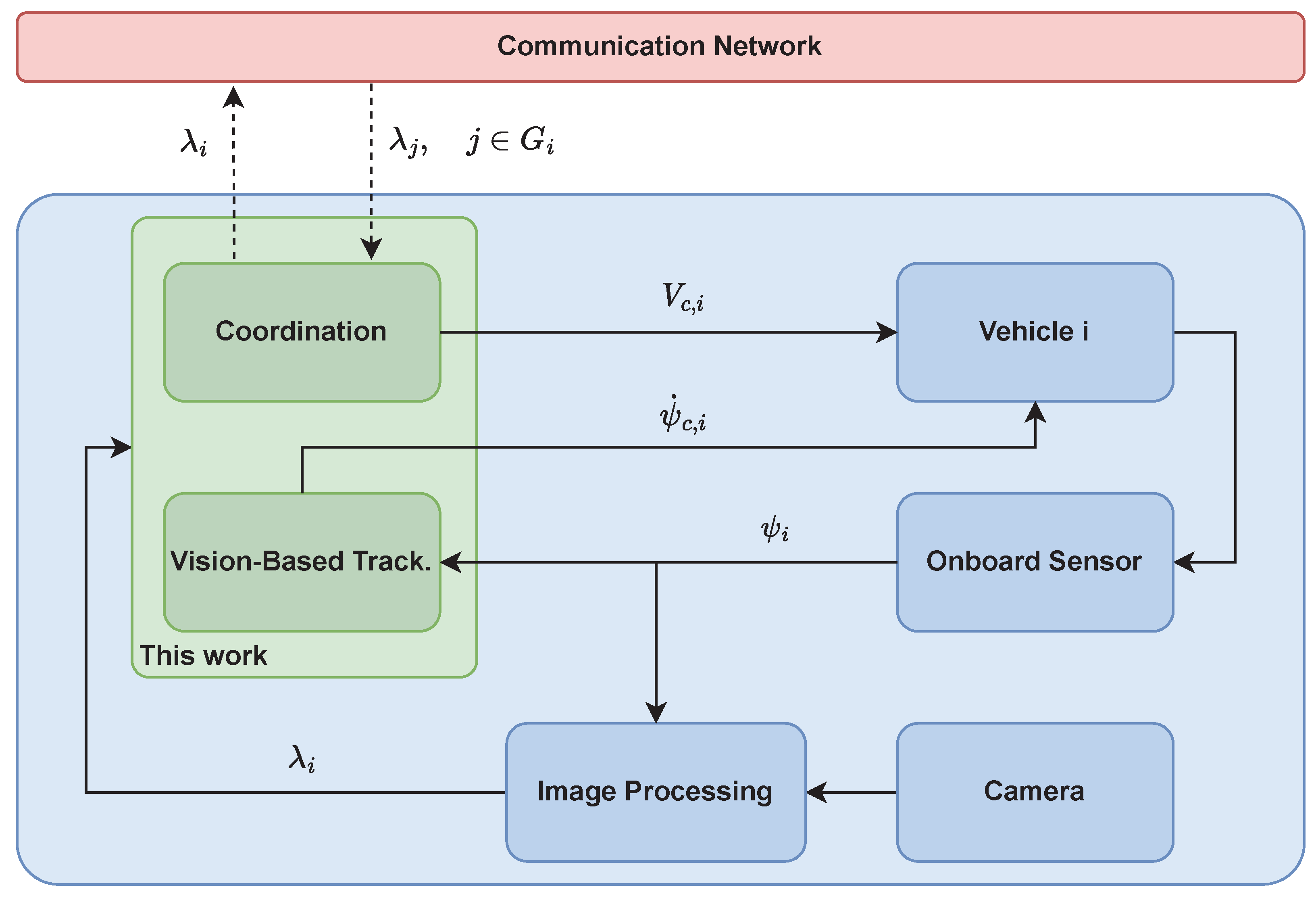
Motivated by these challenges, we describe a solution to the Coordinated Vision-Based Tracking (CVBT) problem. The objective of this work is to enable a set of n vehicles, with dynamics described by the kinematic car model (i.e., Dubins’ car), to orbit around (track and monitor) a target while coordinating their phase separation with each other. Figure 1 depicts the control framework adopted in this paper. The work focuses on two main parts. First, we derive a control algorithm for the yaw rate to enable the vehicles involved in the mission to track a (static or moving) target and orbit around it (VBT). Second, we formulate control laws for the speed of each vehicle so that they maintain a predefined space separation while orbiting around the target (coordination).
At the VBT level, we show that VBT is achieved by using only vehicle-to-target relative line-of-sight (LOS) angles, which can be obtained from the visual measurement. This reduces the computational load required to acquire more complex information, such as the target’s position and velocity. The solution to the VBT problem presented in this paper builds on previous papers [21,22], where the authors demonstrate that the proposed control algorithm guarantees exponential convergence and ultimate boundedness of the VBT error in the case of static and moving targets. One fundamental assumption made in [21] is that the velocity of the unmanned vehicle is constant. In [22], such an assumption is relaxed and convergence of the VBT error to zero is guaranteed as long as the speed of the vehicle is lower and upper bounded by some constants. However, the work in [22] assumes that the UxV is equipped with an ideal inner-loop autopilot (AP), which guarantees that the difference between commanded and actual angular rates is always identical to zero. In the present paper, we address a more realistic case, where the AP can only ensure that such a difference is bounded. It is shown that the VBT algorithm is robust to non-perfect tracking of the VBT input commands. Performance of the outer-loop VBT controller is derived as a function of the performance of the inner-loop AP.
At the coordination level, motivated by [14], where the authors propose a solution to the cooperative path-following problem, we propose a control law for the speeds of the UxVs and show that coordination can be achieved by allowing the vehicles to exchange minimum information (the LOS angle only) between each other over a communication network. Performance of the coordination algorithm is analyzed, while taking into account non-ideal communication scenarios (such as failures, drop-outs, and switching topology). We further extend the coordination result by considering non-perfect tracking of the speed commands. We show that the controller’s performance is guaranteed as long as the difference between the commanded and actual speed of the vehicles remains bounded.
The main features of this paper are as follows: (i) VBT is achieved by using only a UxV-target-relative (LOS) angle; (ii) performance of the overall control architecture is guaranteed against communication failures among the UxVs and non-ideal tracking of the reference control commands by the autopilot.
The paper is organized as follows: Section 2 formulates the CVBT problem; it describes the kinematics of the systems of interest and introduces a set of assumptions and limitations on the onboard autopilot, as well as on the supporting communication network. Section 3 presents a control algorithm that solves the problem at hand. Section 4 illustrates the simulation results. Finally, conclusions are summarized in Section 5. Theoretical proofs of the results are reported in the Appendix A, Appendix B, Appendix C, Appendix D and Appendix E.
2. Problem Formulation
In what follows, we first consider a single UxV and characterize the dynamics of the kinematic errors, describing the VBT approach that was previously presented in [21]. Second, following a decentralized coordination strategy similar to the one presented in [23], we consider the case of multiple UxVs by introducing a set of appropriate coordination variables, along with assumptions and limitations on a given communication network. Table 1 lists the symbols and their definitions for clarity.
2.1. Vision-Based Tracking
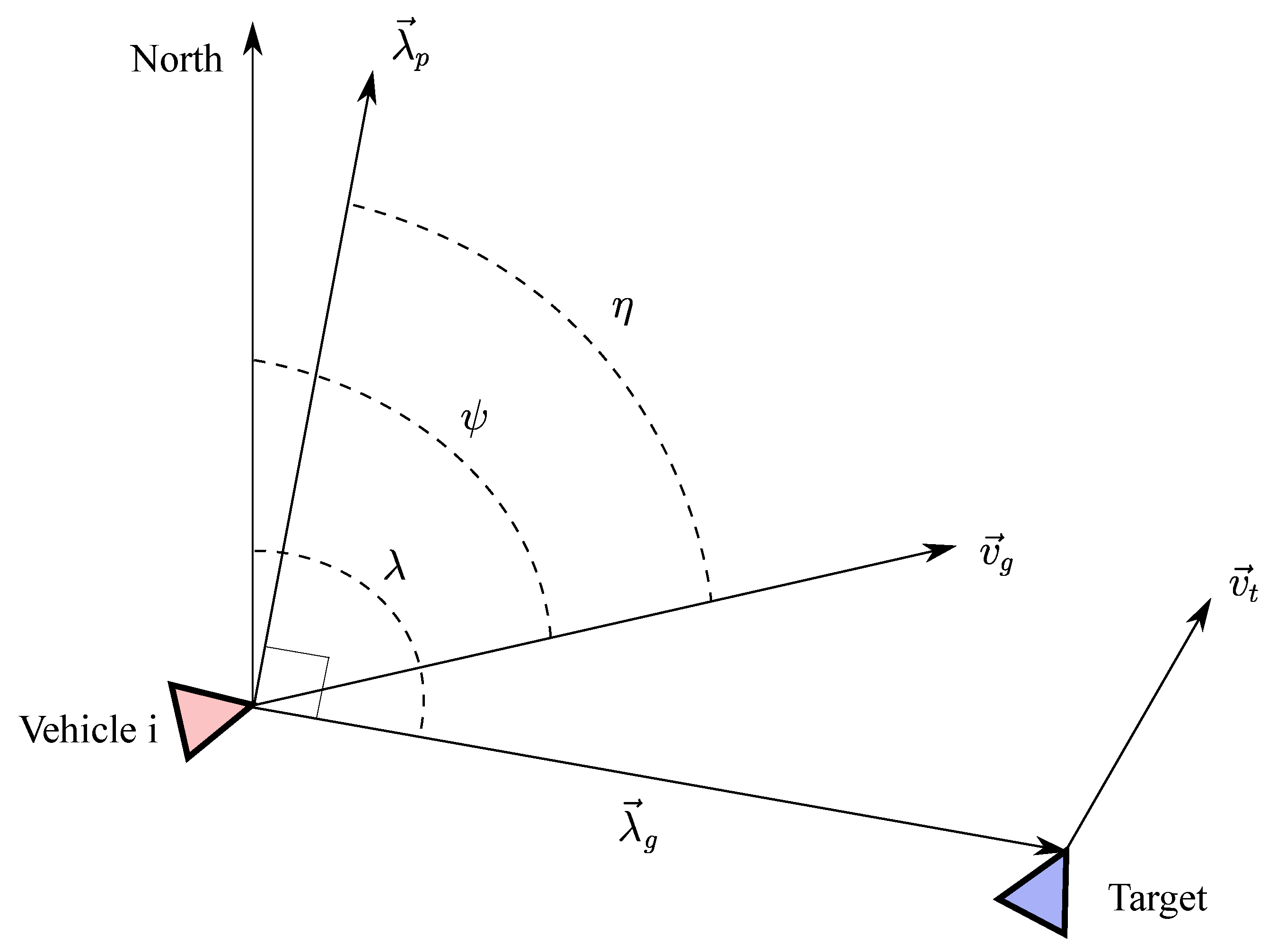
Consider the horizontal projection of the UxV and target-relative kinematics in the inertial frame illustrated in Figure 2. Let and be the UxV’s velocity vector and heading angle, respectively. Let be the magnitude of . Let be the speed of the target and be its heading angle. Let be the horizontal distance between the UxV and the target. Let be the LOS phase angle, let denote the LOS vector, and let be the vector perpendicular to . Finally, let denote the angle between and , which can be written as
Since the rotational speed of the LOS can be expressed as
one can compute the derivative of Equation (1):
Next, define .
In what follows, plays the role of guidance tracking error. Obviously, if , then , and it follows from Equation (1) that the angle between the UxV velocity vector and the LOS vector equals rad. This results in the UxV orbiting around the target, which constitutes part of the control objective. In fact, to accomplish VBT, the control law must also enable the UxV to orbit along a desired circle. This can be achieved when driving the horizontal range to a desired constant value, . By projecting the horizontal components of the UxV velocity vector onto the LOS, one can express the dynamics of as follows:
Finally, by defining , we can write the dynamics of the VBT error states
where . Before providing a formal statement of the problem at hand, we give a set of assumptions that must be satisfied:
Assumption 1.
The speed of the UxV is bounded as follows:
Assumption 2.
The speed of the target to be tracked satisfies
Assumption 3.
The UxV is equipped with an autopilot capable of following speed and yaw rate commands, and . The tracking performance of the autopilot satisfies
for all and for some .
Finally, the VBT control problem can be defined as follows:
Problem 1.
Vision-Based Tracking (VBT): Consider a UxV and a target with speeds satisfying Assumptions 1 and 2. Assume that the UxV is equipped with an autopilot satisfying Assumption 3. Then, the objective of VBT is to define a control law for the commanded angular velocity of the UxV, , such that the error vector , with dynamics in Equation (3), converges to a neighborhood of zero.
Remark 1.
The control algorithm utilizes feedback from image processing software (centroid position in camera frame) and an on-board inertial measurement unit, typical for modern autopilots. Hence, only the line of sight (LOS) to the target is assumed to be known, justifying the use of the term “vision-based tracking”. The crucial aspect of the approach is achieving convergence of the horizontal range to a desired value , without knowledge of the actual range , target position, or velocity.
2.2. Coordination
Consider now a set of n UxVs and let , , and be the speed, the heading angle, and the LOS angle of the i-th vehicle (), respectively. Furthermore, let and be its VBT errors with the dynamics described in Equation (3). The objective of coordination is to drive the difference between the UxVs LOS phase angles to a desired value, in order to maintain a desired phase separation. Thus, we consider the i-th and j-th vehicles to be coordinating at time t if their LOS angles satisfy the condition
where is the desired separation in terms of LOS angle. Finally, without loss of generality, it is convenient to set ; when a specific phase shift is desired, can be assigned a desired constant value. Therefore, the coordination problem for multiple UxVs reduces to achieving .
To guarantee coordination, the states have to be exchanged between the UxVs over a communication network. In this paper, we use the notation and tools from algebraic graph theory. Introduction to the material and further relevant reading can be found in [24]. Let be the Laplacian matrix of the communication graph . Let be such that and , with . Let denote the set of vehicles positioned in a neighborhood of the i-th UxV. Now, we can define a set of assumptions that the communication network must satisfy [25]:
Assumption 4.
The i-th UxV can only communicate with the neighboring set .
Assumption 5.
The communication between two vehicles is bidirectional, with no time delays.
Assumption 6.
The connectivity of the communication graph satisfies
where has the same spectrum of without the eigenvalue , and the parameters describe the quality of service of the communication network.
It is worth noting that Assumption 6 stipulates that the communication graph is only required to be connected in an integral sense over the time range T rather than pointwise in time. In fact, the graph may be disconnected during some interval of time or may even fail to be connected at all times. In this sense, it is general enough to capture packet dropouts, loss of communication, switching topologies, etc. Small values of T and large values of indicate better quality of the communication network.
Finally, the coordination problem can be defined as follows:
Problem 2.
Coordination: Consider a set of n UxVs with speed satisfying Assumption 1 and a target with speed satisfying Assumption 2. Assume that the vehicles are equipped with an autopilot satisfying Assumption 3. Finally, suppose that the UxVs are supported by a communication network satisfying Assumptions 4–6. Then, the objective is to design feedback control laws for the commanded speeds such that the difference between the LOS angles of the n UxVs converge to a neighborhood of zero, i.e.,
and such that the speeds of the vehicles converge to predefined constant values, i.e.,
3. Main Result
In this section, we first present the outer-loop nonlinear controller that uses the angular velocity to solve Problem 1. Then, we formulate a control law for the speed commands , which solves Problem 2.
3.1. Vision-Based Tracking
Recall from Section 2 that the main objective of the VBT control algorithm is to drive the states to a neighborhood of zero. To this end, we propose the following guidance law [21]:
Then, the solution to the VBT problem for a single UxV can be summarized in the following Lemma:
Lemma 1.
Vision-Based Tracking (VBT): Consider a UxV with speed satisfying Assumption 1 and a moving target with speed satisfying Assumption 2. Let the commanded angular rate be governed by Equation (4) and assume that the vehicle is equipped with an autopilot satisfying Assumption 3. Moreover, assume that at time the error vector satisfies
with ; satisfies
with P and W being positive definite matrices, and
Then, if the velocity of the target and the angular speed tracking performance of the autopilot (i.e., ) satisfy
the VBT error , with the dynamics described in Equation (3), is ultimately bounded with bound
Corollary 1.
Under the assumptions stated in Lemma 1, if the velocity of the target is and the autopilot has ideal performance of (i.e., ), the VBT error converges exponentially to zero as follows:
Proof .
The proofs of Lemma 1 and Corollary 1 are given in Appendix A and Appendix B, respectively.
3.2. Coordinated Vision-Based Tracking
To drive the LOS angles of the UxVs to the same increasing value, the speed of the vehicles is adjusted based on the coordination information exchanged over the communication network. Since, by assumption, each UxV can only communicate with a neighboring set of vehicles, denoted as , we let the commanded velocity for the i-th vehicle be governed by
where
with vehicle 1 elected as leader of the fleet, and . Note that are constant desired speeds that satisfy in order to maintain the same turn rate around the target. Moreover, the following inequalities must hold to guarantee feasibility of the mission:
, where .
Remark 2.
Parameter δ guarantees that a margin is left between the minimum (and maximum) UxV’s velocity and the desired speed, therefore ensuring the existence of a solution for the coordination problem. In fact, assume that the desired speed for the i-th UxV is . It follows that, if the vehicle is required to slow down in order to coordinate with the rest of the fleet, it would not be possible since no margin is left between the desired and minimum feasible velocities.
Next, we define the coordination error vector as
where
where and
Note that, from the properties of Q, if at time t we have , then , which implies that for all . Moreover, if at the same time , then the commanded speed of each vehicle is equal to its desired constant speed, which is
Before stating the main result of the paper, let us define as and
where P is a positive definite matrix, satisfies Equation (6), and
where ; ; and some positive , and .
Finally, the main result is stated in the following Theorem:
Theorem 1.
if the velocity of the target and the angular rate tracking performance of the autopilot (i.e., ) satisfy
where and are positive constants.
Coordinated Vision-Based Tracking (CVBT): Consider a set of n UxVs and a target with speed satisfying Assumption 2. Let the commanded angular rate of the UxVs be governed by Equation (4), and let the commanded speed be governed by Equation (8). Assume that the UxVs are equipped with autopilots satisfying Assumption 3. Suppose that the UxVs communicate over a network satisfying Assumptions 4–6. If at time the VBT error and the coordination error satisfy
and
respectively, then we have the following:
- (i)
- The velocities of the UxVs satisfy Assumption 1;
- (ii)
- The VBT error , with dynamics described in Equation (3), is ultimately bounded with bound
- (iii)
- The coordination error vector defined in Equation (10) satisfies the following bound:
Corollary 2.
where are positive constants, with rate of convergence , with , and
Under the same assumptions stated in Theorem 1, if the velocity of the target is , and the autopilot has ideal performance (i.e., ), we have the following:
- (i)
- The velocities of the UxVs satisfy Assumption 1;
- (ii)
- (iii)
- The coordination error vector defined in Equation (10) converges exponentially to zero as follows:
Proof .
The proofs of Theorem 1 and Corollary 2 are given in Appendix C and Appendix D, respectively.
Remark 3.
The maximum guaranteed rate of convergence can be obtained by letting , which is
Moreover, it is worth noticing that if one modifies the control laws given in Equation (9) as follows:
i.e., all the UxVs involved in the mission are leaders; then, one can show [23] that the rate of convergence reduces to
This implies that the rate of convergence depends on the quality of the communication network, and it scales with the number of vehicles.
4. Simulation Results
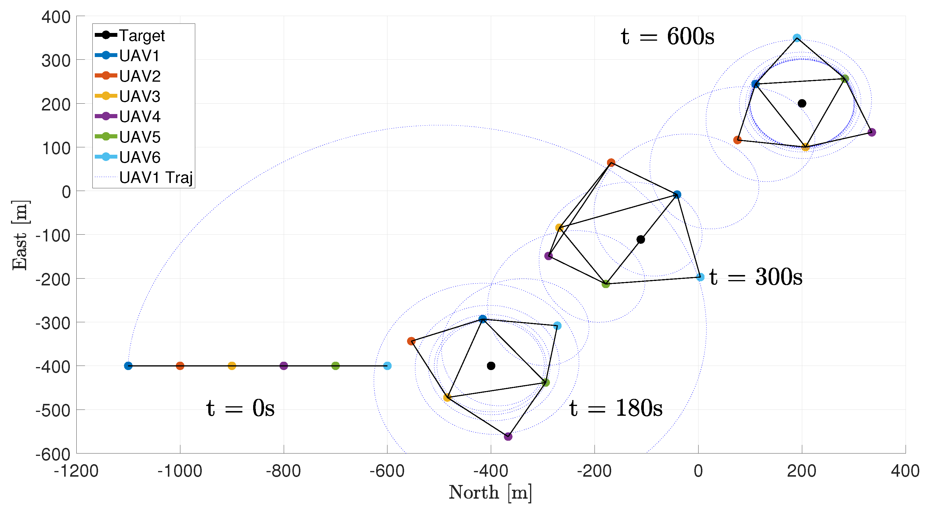
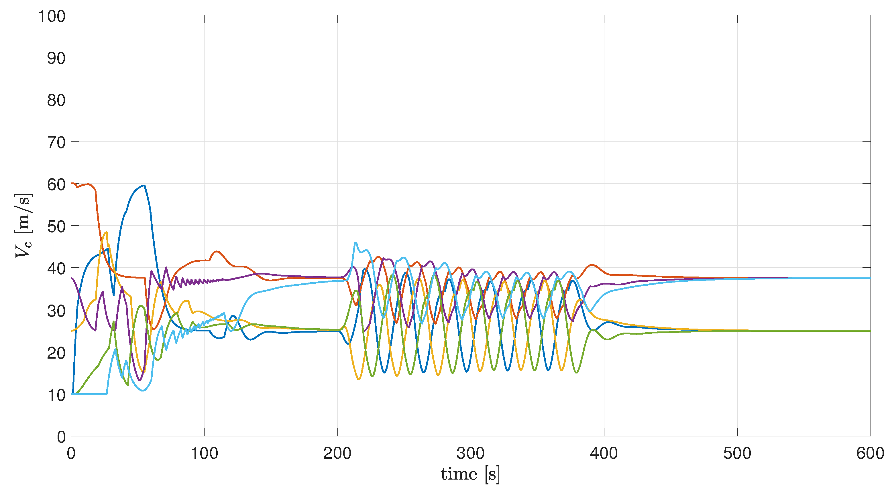
This section presents the simulation results. In the proposed scenario, six UxVs are asked to rotate around a target along two orbits of different radius, while maintaining a phase separation of from each other. In particular, UxV1—elected as the leader—UxV3, and UxV5 are required to rotate on an orbit of radius , while UxV2, UxV4, and UxV6 rotate on an orbit of radius . The desired speeds at which the UxVs are asked to converge are and .
We assume that the vehicles can only communicate with each other when the distance between them is less than . All-to-all communication is never achieved throughout the mission. In Figure 3, the black lines connecting vehicle i and vehicle j indicate that the two UxVs are communicating. For clarity of presentation, these lines are shown only at four different time instances ().
To illustrate the performance of the CVBT controller in the presence of non-ideal tracking of reference commands, we implemented a proportional controller as follows
with gains , and time delay . The time delay is intentionally introduced to simulate the effects of real-world delays that can impact the performance of an unmanned vehicle’s autopilot system.
The control gains of the CVBT controller have been chosen as follows: . The imposed speed limits are and .
Mission
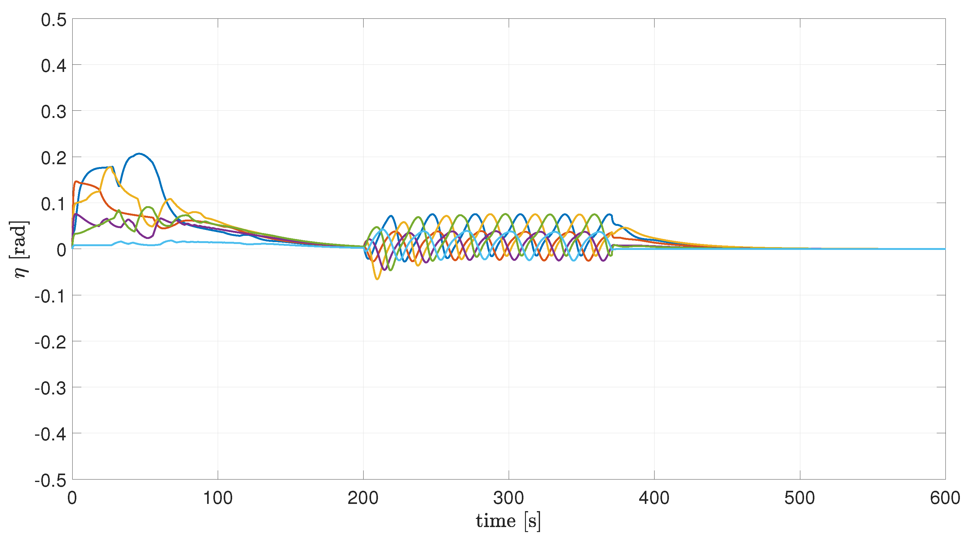
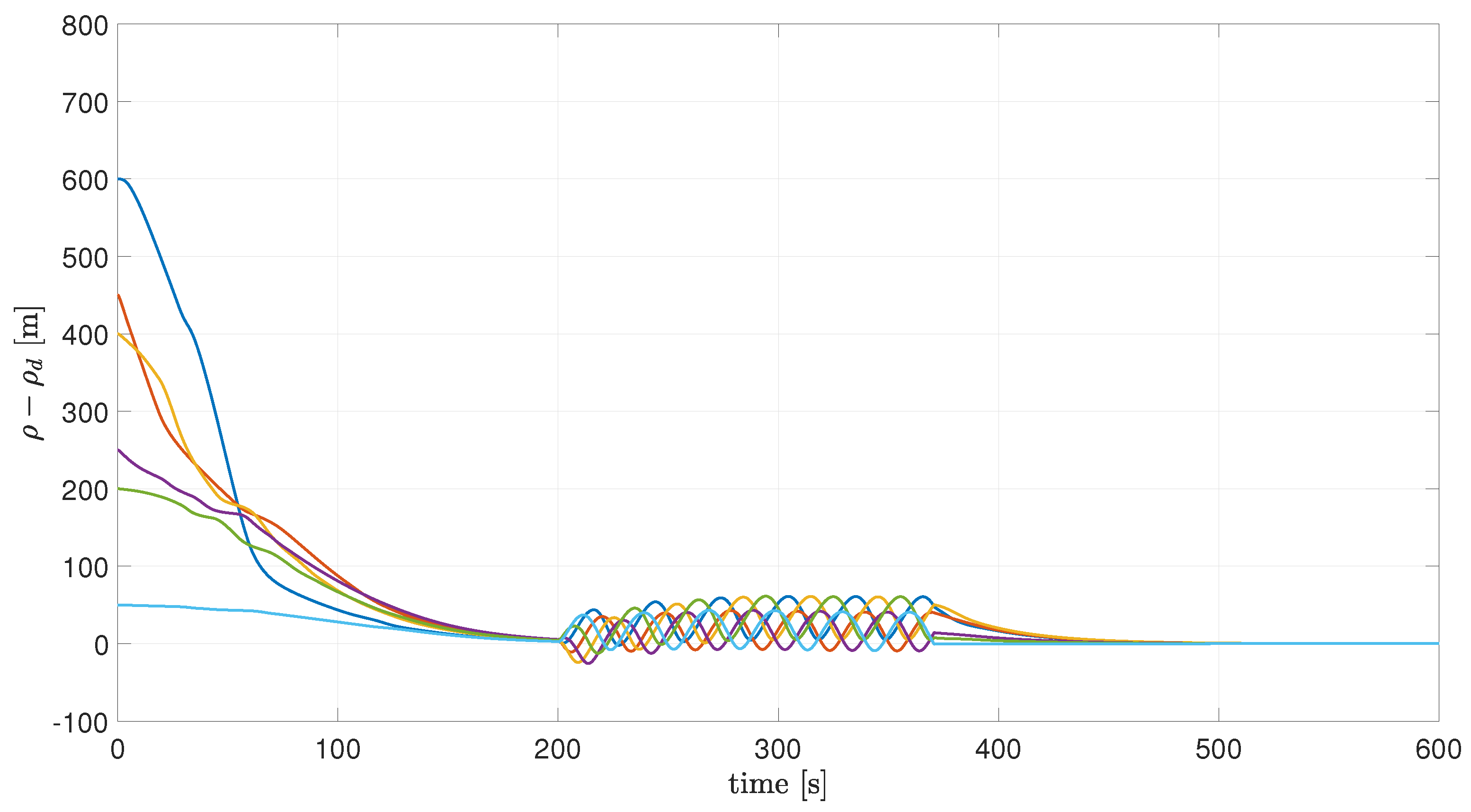
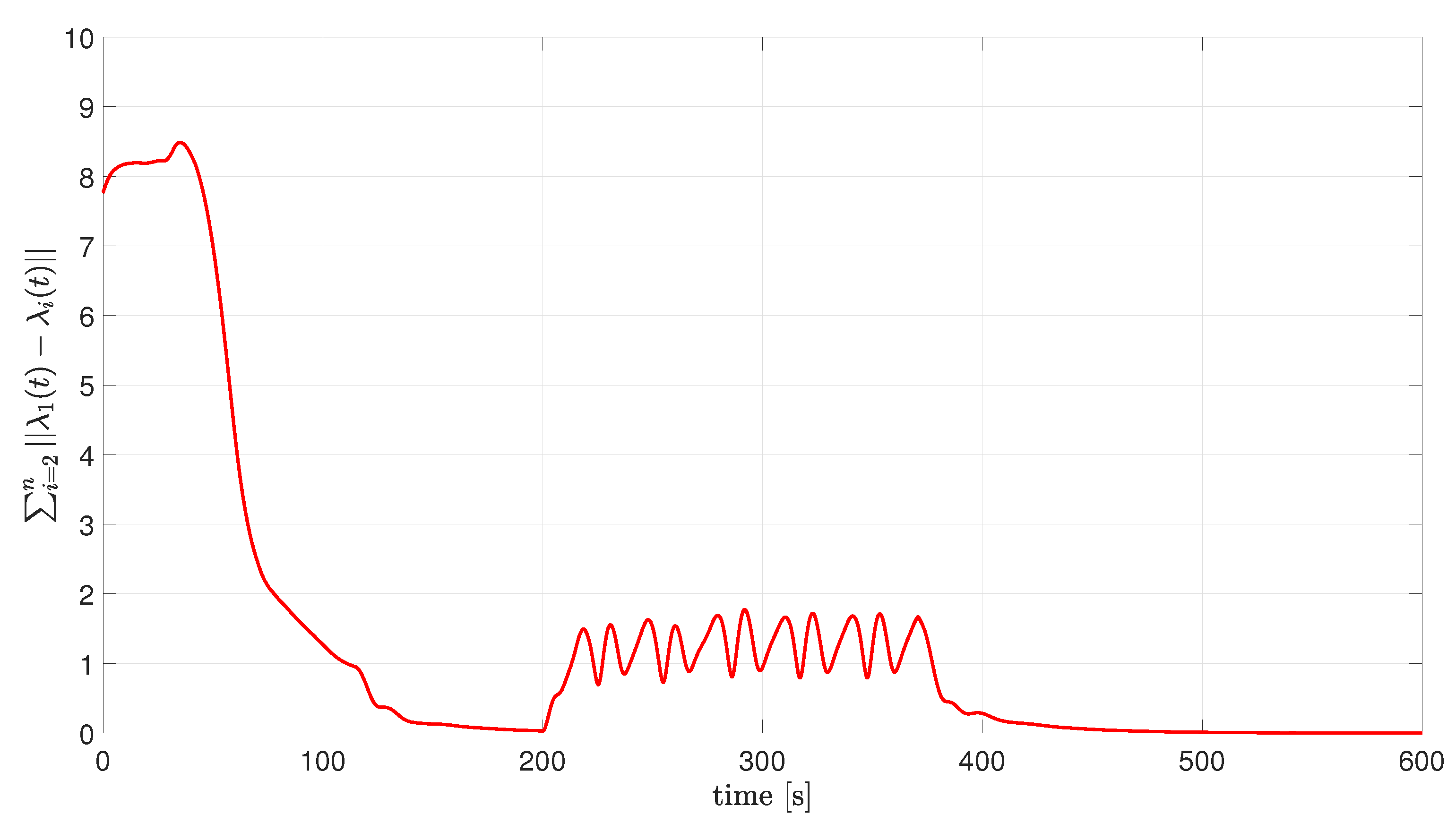
At , the target is positioned at with velocity , and the UxVs are positioned in a straight-line formation near the target, as depicted in Figure 3. When the mission begins, the UxVs start approaching the desired orbits with different speed profiles. Figure 4 and Figure 5 show the convergence to a neighborhood of zero of the VBT error. Figure 6 and Figure 7 illustrate the coordination error and the actual speeds. The slow rate of convergence depends on the facts that the UxVs start the mission far away from each other and each vehicle is able to communicate with only few of its neighbors (see Figure 3, black lines).
At , the target starts moving in the northeast direction at a speed of . As it can be seen in Figure 7, the speeds of the vehicles oscillate around the desired values. The reason is that the trajectory of the UxVs at this time is not a circular orbit, as it is in the case of a stationary target (this can be noted from the trajectory of UxV1 depicted in Figure 3), and following this trajectory requires oscillatory (linear and angular) velocity commands. Finally, Figure 4, Figure 5 and Figure 6 show the oscillatory behavior of the VBT and the coordination errors, which, however, remain bounded as expected.
At , the target reaches position and stops (i.e., ). Again, the speeds converge to the desired values, while the VBT and the coordination error converge close to zero.
A video of these results and the Matlab code used to generate the plots can be found at the following link: https://github.com/venanziocichella/Cooperative-Vision-Based-Tracking (accessed on 2 March 2023).
5. Conclusions
In this paper, a solution for the coordinated vision-based tracking problem is given. The proposed control laws enable n unmanned vehicles (UxVs) to move around a target along n desired orbits, while coordinating with each other (i.e., maintaining a desired phase shift). The yaw rate is used to solve the vision-based tracking problem. The coordination between the UxVs is achieved by adjusting the speed of each vehicle. Non-perfect tracking performance of an on-board autopilot is considered. First, a solution to the vision-based tracking problem is given considering the case of a single UxV. Second, we provide a solution to the coordination problem. The simulation results validate the theoretical findings.
Author Contributions
Conceptualization, V.C. and I.K.; methodology, V.C. and I.K.; software, V.C and I.K.; validation, V.C and I.K.; investigation, V.C. and I.K.; resources, V.C. and I.K.; writing—original draft preparation, V.C. and I.K.; writing—review and editing, V.C and I.K.; supervision, V.C. and I.K.; project administration, V.C. and I.K.; funding acquisition, V.C. and I.K. All authors have read and agreed to the published version of the manuscript.
Funding
Venanzio Cichella was supported by Amazon and by the Office of Naval Research (grants N000141912106 and N000142112091). Isaac Kaminer was supported by the Office of Naval Research (grants N0001421WX01974, N0001419WX00155, N0001422WX01906) and NPS CRUSER.
Institutional Review Board Statement
Not applicable.
Informed Consent Statement
Not applicable.
Data Availability Statement
Not applicable.
Conflicts of Interest
The authors declare no conflict of interest.
Appendix A. Proof of Lemma 1
Consider System (3). Add and subtract in the first equation, and substitute the control law in Equation (4) to obtain
After simple algebraic manipulations, we can rewrite the previous system of equations as
where ,
Next, consider the following Lyapunov function
Letting
and noting that , the derivative of the Lyapunov function can be computed as
Defining such that , and recalling Assumption 3 and the bound in Equation (A1), one can write
It follows that if
Finally, we can conclude that if and are sufficiently small and satisfy Condition (14), then , which completes the proof.
Appendix B. Proof of Corollary 1
The proof follows easily from the proof of Lemma 1 given in Appendix A. Consider the candidate Lyapunov function introduced in Equation (A2). Letting and , from Equation (A3) it follows that
Applying the comparison lemma, we obtain
Appendix C. Proof of Theorem 1
The proof of Theorem 1 unfolds in two main steps:
- Part (b): We prove that if the initial conditions of the vision-based tracking error and coordination error satisfy and , respectively, then the control law for the speed given in Equation (8), together with the bounds presented in Assumption 3, satisfy Assumption 1 ; therefore, .
Part (b) implies that Part (a) holds , thus proving Theorem 1.
Appendix C.1. Part (a)
First, we note that the result given in Equation (13) follows directly from Lemma 1 if Assumption 1 is satisfied. Thus, we can state that
Second, from [25] Lemma 5, it follows that if the matrix satisfies Assumption 6; then, a generic system with dynamics
converges exponentially to zero as follows:
with . This implies that ([26] Theorem 4.12), for any constants and satisfying , there exists a continuously differentiable, symmetric, positive definite matrix that satisfies the following inequalities:
Now, let us consider the first derivative of , which can be rewritten as follows:
where . Substituting the control law given by Equation (8), we obtain
which can be written in vector form as
with
and , and being the set of the individual variables collected in a column vector (e.g., ).
Similarly, by defining and , Equation (9) can be written in vector form as
Then, consider the coordination error vector , where
Differentiating with respect to time, we obtain
Similarly, differentiating , we have
Combining Equations (A7) and (A8), we can write the dynamics of the coordination error vector in compact form as follows:
where
Let us apply the change of variables
with dynamics given by
Next, consider the following Lyapunov function candidate
with
where M satisfies Equations (A5) and (A6). Noting that , we can state that is bounded as follows:
Computing the time derivative of , and letting , we obtain
Using Equation (A6), , and , we can write
At this point, one can show (see Appendix E) that, for some choice of , and , the following inequality is satisfied:
where , which allows us to write
Appendix C.2. Part (b)
We will prove the claim by contradiction. Assume that at some time the Vision-Based Tracking error of the i-th UxV is such that . Thus, there exists a time such that
while
The choice of k and in Appendix E, together with the definition of , implies that there exists a positive constant such that ; therefore, the velocity command given in (8) is well-defined . Moreover, from the proof given in Appendix C, Part (a), it follows that the coordination error at time satisfies
where, by assumption, with
Consider now the speed of the i-th vehicle at time given by
Noting that satisfies
we can find the following bound for the speed
Hence, from the result in Equation (A19), from the choice of and , and for sufficiently small values of , the following bound is verified at time :
Using the proof given in Appendix A, we can show that , thus contradicting the claim in Equation (A17).
Appendix D. Proof of Corollary 2
Since , from Corollary 1, we obtain the following result
Notice that from it follows that
Using Equation (A20), we can write
Therefore, combining Equation (A24) with the previous two inequalities, and letting
we obtain
thus proving Corollary 2.
Appendix E. Proof of Inequality Equation (A13)
To prove inequality Equation (A13), we need to show that the following matrix is positive semi-definite:
Equation (A27) is satisfied if the following holds:
Letting and , the previous inequality reduces to
Now, consider the term and recall that
Letting , noting that , choosing , and recalling the fact that , one can show that the following relation holds:
Therefore, Equation (A29) is satisfied if the following inequality is true:
which is guaranteed from the choice .
Using the fact that , , and after straightforward computations, the previous inequality reduces to
Finally, substituting
and choosing
we can show that Equation (A30) is verified, which completes the proof.
References
- Mcfadyen, A.; Mejias, L. A survey of autonomous vision-based see and avoid for unmanned aircraft systems. Prog. Aerosp. Sci. 2016, 80, 1–17. [Google Scholar] [CrossRef]
- Al-Kaff, A.; Armingol, J.M.; de La Escalera, A. A vision-based navigation system for Unmanned Aerial Vehicles (UAVs). Integr. Comput. Aided Eng. 2019, 26, 297–310. [Google Scholar] [CrossRef]
- Asl, H.J. Robust vision-based tracking control of VTOL unmanned aerial vehicles. Automatica 2019, 107, 425–432. [Google Scholar]
- Cichella, V.; Kaminer, I.; Dobrokhodov, V.; Hovakimyan, N. Coordinated vision-based tracking for multiple UAVs. In Proceedings of the 2015 IEEE/RSJ International Conference on Intelligent Robots and Systems (IROS), Hamburg, Germany, 28 September–2 October 2015; IEEE: New York, NY, USA, 2015; pp. 656–661. [Google Scholar]
- Lawrence, A. Modern Inertial Technology: Navigation, Guidance, and Control; Springer: Berlin/Heidelberg, Germany, 1998. [Google Scholar]
- Redding, J.D.; McLain, T.W.; Beard, R.W.; Taylor, C.N. Vision-based target localization from a fixed-wing miniature air vehicle. In Proceedings of the American Control Conference, Minneapolis, MN, USA, 14–16 June 2006; IEEE: New York, NY, USA, 2006; p. 6. [Google Scholar]
- Campbell, M.E.; Wheeler, M. Vision-based geolocation tracking system for uninhabited aerial vehicles. J. Guid. Control. Dyn. 2010, 33, 521–532. [Google Scholar] [CrossRef]
- Bar-Shalom, Y. Tracking and Data Association; Academic Press Professional, Inc.: Cambridge, MA, USA, 1987. [Google Scholar]
- Ljung, L. Asymptotic behavior of the extended Kalman filter as a parameter estimator for linear systems. Autom. Control. IEEE Trans. 1979, 24, 36–50. [Google Scholar] [CrossRef] [Green Version]
- Ghyzel, P.A. Vision-Based Navigation for Autonomous Landing of Unmanned Aerial Vehicles. Ph.D. Thesis, Naval Postgraduate School, Monterey, CA, USA, 2000. [Google Scholar]
- Valasek, J.; Gunnam, K.; Kimmett, J.; Junkins, J.L.; Hughes, D.; Tandale, M.D. Vision-based sensor and navigation system for autonomous air refueling. J. Guid. Control. Dyn. 2005, 28, 979–989. [Google Scholar] [CrossRef]
- Aicardi, M.; Casalino, G.; Bicchi, A.; Balestrino, A. Closed loop steering of unicycle like vehicles via Lyapunov techniques. Robot. Autom. Mag. IEEE 1995, 2, 27–35. [Google Scholar] [CrossRef]
- Frew, E.W.; Lawrence, D.A.; Morris, S. Coordinated standoff tracking of moving targets using Lyapunov guidance vector fields. J. Guid. Control. Dyn. 2008, 31, 290–306. [Google Scholar] [CrossRef]
- Kaminer, I.; Pascoal, A.M.; Xargay, E.; Hovakimyan, N.; Cichella, V.; Dobrokhodov, V. Time-Critical Cooperative Control of Autonomous Air Vehicles; Butterworth-Heinemann: Oxford, UK, 2017. [Google Scholar]
- Cichella, V.; Choe, R.; Mehdi, S.B.; Xargay, E.; Hovakimyan, N.; Dobrokhodov, V.; Kaminer, I.; Pascoal, A.M.; Aguiar, A.P. Safe coordinated maneuvering of teams of multirotor unmanned aerial vehicles: A cooperative control framework for multivehicle, time-critical missions. IEEE Control Syst. Mag. 2016, 36, 59–82. [Google Scholar]
- Mesbahi, M.; Hadaegh, F.Y. Formation flying control of multiple spacecraft via graphs, matrix inequalities, and switching. J. Guid. Control. Dyn. 2001, 24, 369–377. [Google Scholar] [CrossRef]
- Pereira, F.L.; De Sousa, J.B. Coordinated control of networked vehicles: An autonomous underwater system. Autom. Remote Control 2004, 65, 1037–1045. [Google Scholar] [CrossRef] [Green Version]
- Stipanović, D.M.; Inalhan, G.; Teo, R.; Tomlin, C.J. Decentralized overlapping control of a formation of unmanned aerial vehicles. Automatica 2004, 40, 1285–1296. [Google Scholar] [CrossRef]
- Ma, L.; Hovakimyan, N. Vision-based cyclic pursuit for cooperative target tracking. J. Guid. Control. Dyn. 2013, 36, 617–622. [Google Scholar] [CrossRef]
- Ma, L.; Hovakimyan, N. Cooperative target tracking with time-varying formation radius. In Proceedings of the European Control Conference, Linz, Austria, 15–17 July 2015; IEEE: New York, NY, USA, 2015. [Google Scholar]
- Dobrokhodov, V.; Kaminer, I.; Jones, K.; Ghabcheloo, R. Vision-based tracking and motion estimation for moving targets using unmanned air vehicles. J. Guid. Control. Dyn. 2008, 31, 907–917. [Google Scholar] [CrossRef]
- Cichella, V.; Kaminer, I.; Dobrokhodov, V.; Hovakimyan, N. Cooperative Vision-Based Tracking of Multiple UAVs. In Proceedings of the AIAA Guidance, Navigation, and Control Conference, Boston, MA, USA, 19–22 August 2013. [Google Scholar]
- Xargay, E.; Kaminer, I.; Pascoal, A.; Hovakimyan, N.; Dobrokhodov, V.; Cichella, V.; Aguiar, A.P.; Ghabcheloo, R. Time-Critical Cooperative Path Following of Multiple Unmanned Aerial Vehicles over Time-Varying Networks. AIAA J. Guid. Control. Dyn. 2013, 36, 499–516. [Google Scholar] [CrossRef] [Green Version]
- Biggs, N. Algebraic Graph Theory; Cambridge University Press: New York, NY, USA, 1993. [Google Scholar]
- Panteley, E.; Loría, A. Uniform Exponential Stability for Families of linear Time-Varying Systems. In Proceedings of the IEEE Conference on Decision and Control, Sydney, Australia, 12–15 December 2000; pp. 1948–1953. [Google Scholar]
- Khalil, H.K. Nonlinear Systems; Prentice Hall: Englewood Cliffs, NJ, USA, 2002. [Google Scholar]
Figure 1.
Coordinated vision-based target tracking—general framework.

Figure 2.
Vision-based target tracking—problem formulation.

Figure 3.
Coordinated vision-based tracking mission—2D paths.

Figure 4.
Vision-based tracking error for each vehicle.

Figure 5.
Vision-based tracking error for each vehicle.

Figure 6.
Coordination error.

Figure 7.
Actual speeds of the vehicles.


Table 1.
Symbols and definitions.
| Symbol | Definition |
|---|---|
| UxV | Unmanned (ground, aerial, underwater, surface) vehicle |
| Inertial frame | |
| , | Speed and velocity of the UxV at time t |
| , | Speed and angular rate commands for UxV i at time t |
| Heading angle of the UxV at time t | |
| , | Speed and heading angle of the UxV at time t |
| Horizontal distance between UxV and target at time t | |
| Line of sight phase angle at time t | |
| Vision-based angle tracking error at time t | |
| Desired range | |
| Vision-based distance tracking error at time t | |
| Vision-based tracking error vector at time t | |
| Neighborhood of vehicle i at time t | |
| Communication graph | |
| Laplacian of the graph at time t | |
| Parameters representing the quality of the communication network | |
| Coordination error vector at time t | |
| Heterogeneity parameter between nodes i and j at time t |
Disclaimer/Publisher’s Note: The statements, opinions and data contained in all publications are solely those of the individual author(s) and contributor(s) and not of MDPI and/or the editor(s). MDPI and/or the editor(s) disclaim responsibility for any injury to people or property resulting from any ideas, methods, instructions or products referred to in the content. |
© 2023 by the authors. Licensee MDPI, Basel, Switzerland. This article is an open access article distributed under the terms and conditions of the Creative Commons Attribution (CC BY) license (https://creativecommons.org/licenses/by/4.0/).
Share and Cite
MDPI and ACS Style
Cichella, V.; Kaminer, I. Coordinated Vision-Based Tracking by Multiple Unmanned Vehicles. Drones 2023, 7, 177. https://0-doi-org.brum.beds.ac.uk/10.3390/drones7030177
AMA Style
Cichella V, Kaminer I. Coordinated Vision-Based Tracking by Multiple Unmanned Vehicles. Drones. 2023; 7(3):177. https://0-doi-org.brum.beds.ac.uk/10.3390/drones7030177
Chicago/Turabian StyleCichella, Venanzio, and Isaac Kaminer. 2023. "Coordinated Vision-Based Tracking by Multiple Unmanned Vehicles" Drones 7, no. 3: 177. https://0-doi-org.brum.beds.ac.uk/10.3390/drones7030177