Benchmarking of Laser Powder Bed Fusion Machines
by
 , , and
Mandaná Moshiri
1,* ,
,
Stefano Candeo
2, 
Simone Carmignato
2,
Sankhya Mohanty
1 and
Guido Tosello
1
1
Department of Mechanical Engineering, Technical University of Denmark, Building 427, Produktionstorvet, DK-2800 Kgs Lyngby, Denmark
2
Department of Management and Engineering, University of Padova, Stradella San Nicola 3, 36100 Vicenza, Italy
*
Author to whom correspondence should be addressed.
J. Manuf. Mater. Process. 2019, 3(4), 85; https://0-doi-org.brum.beds.ac.uk/10.3390/jmmp3040085
Submission received: 14 August 2019
/
Revised: 4 September 2019
/
Accepted: 19 September 2019
/
Published: 1 October 2019
Abstract
:This paper presents the methodology and results of an extensive benchmarking of laser powder bed fusion (LPBF) machines conducted across five top machine producers and two end users. The objective was to understand the influence of the individual machine on the final quality of predesigned specimens, given a specific material and from multiple perspectives, in order to assess the current capabilities and limitations of the technology and compare them with the capabilities of an 11-year-old machine belonging to one of the end users participating in this investigation. The collected results give a clear representation of the status of LPBF technology considering its maturity in terms of process capabilities and potential applications in a production environment.
1. Introduction and State of the Art
For about the last 40 years, additive manufacturing (AM), initially known as rapid prototyping, has experienced huge technological advancements. AM is distinguished from other existing technologies as it presents unparalleled design freedom and the possibility of mass customization [1,2]. Complexity and customization in AM were deeply analyzed by Conner et al. by developing a reference system for products that considered customization, volume, and complexity [3], and by Quinlan et al., who analyzed the capability of AM to provide “complexity for free” and compared this capacity with conventional manufacturing technology [4].
According to the ASTM F42 committee, all AM processes can be classified into the following seven main categories [5]:
- Binder jetting (BJ);
- Direct energy deposition (DED);
- Material extrusion (ME);
- Material jetting (MJ);
- Powder bed fusion (PBF);
- Sheet lamination (SL);
- Vat photopolymerization (VPP).
The applications of AM technologies are numerous across all industries, but their full potential has not yet been exploited [6]. Gu et al. claimed that in the next few years, prototyping production using polymers will no longer be a research focus, since it will reach its full maturity, while the focus will be more on AM techniques for the industrial production of metallic components that cannot be produced easily with conventional technologies [7]. Among the AM technologies that are capable of processing metal materials and are used the most for industrial applications, powder bed fusion—also called selective laser melting (SLM) or laser powder bed fusion (LPBF)—stands out. Today, LPBF technologies have been demonstrated to be among the most versatile AM metal processes, showing the capability of producing metal components that have complex shape and are otherwise impossible to produce by conventional manufacturing technologies [8].
LPBF, as all powder-based systems, produces parts by spreading dry powder on a building platform and scanning the selected areas given by the CAD design, converted in STL format, with a laser. The platform is then lowered by one step, a new layer of powder is spread on the surface and the process starts again. One of the main advantages of LPBF is its relatively high resolution including its internal features [9].
Among the main applications of LPBF are aerospace and aviation engineering, biomedical, and tooling [10].
Several LPBF systems are currently available on the market, each with its own strengths and limitations. However, it is still under debate how much powder bed fusion metal AM is ready for industrial production.
In addition, when considering the broad variety of available metal AM systems, it should be investigated how much the choice of a specific LPBF machine influences the quality of the final products. This is the framework through which the present work tries to give some answers to those questions through a machine benchmarking study.
One of the most detailed works dedicated to the benchmarking of AM machines was conducted by Mahesh et al. in 2002. The study describes benchmarking as a process to identify the “highest standards of excellence for products, services and processes” [11]. Benchmarking is a known method to evaluate the capabilities and limitations of a process, in this case an AM process, but is also a useful instrument to identify optimization approaches and sources of information [12]. In their work, Mahesh and colleagues also proposed for the first time a benchmark classification of AM processes, depending on the main purpose of the benchmark. These were divided into three groups:
- Geometrical benchmark, used to evaluate the geometrical and dimensional accuracy of the additively manufactured products;
- Mechanical benchmark, a standard design of components to evaluate the AM parts’ mechanical properties such as tensile strength, shrinkage, creep properties, etc.; and
- Process benchmark including all the benchmarking artifacts used to optimize the process, for example, to define the best process parameters for a given outcome [11].
Many benchmarking artifacts have been designed and tested in recent years, and a comprehensive review was presented by Rebaioli and Fassi in 2017 [13]. From this extensive review, we recognize the need for a standardized procedure to evaluate AM processes. In their paper from 2014, Moylan et al. attempted to define general rules for a standard artifact: that it should be large enough to evaluate the system performance, but does not consume too much material to be printed. A standard artifact should include small, medium, and large features, and have both holes and bosses. It must be easy to measure and present some real part features [14]. These guidelines, among other considerations, were followed by Moylan et al. for their artifact, which was developed at the National Institute of Standards and Technology (NIST), and was proposed as a standard test artifact for AM machines [15].
What appears to be clear through the literature review of benchmarking is that most of the studies and recommendations have not focused on a specific AM technology. In fact, the aim was mostly to compare different technologies. In Table 1, some selected examples of benchmarking research that was particularly important for understanding AM processes and comparisons are presented.
Goals and Structure of the Paper
In the present work, the aim was not to compare different AM technologies, but rather to compare different machines belonging to the same LPBF family. The aim was to understand the performance of different systems and assess the current capabilities and limitations of the process. For these reasons, an innovative artifact design was formulated to highlight the differences and similarities among the considered systems.
The rest of this paper is structured as follows: in Section 2, the design of this extensive benchmarking project is summarized, referring to a previous paper where this design was introduced by Moshiri et al. [27]. Next, in Section 3, the methodology followed in this work is explained in detail, considering both the data transfer with the participants who took part and the actual analysis undertaken on the specimens. For confidentiality, the identities of the participants are not disclosed; but consist of five current state-of-the-art LPBF machine producers and two end users whose production LPBF systems are used daily. Finally, one machine placed at one of the end users was 12 years old. This system was considered in order to highlight the degree of performance that more modern systems have reached after approximately one decade of process development and advancements. In Section 4, the collected results are presented and the various systems are compared. Our final remarks and conclusions are presented in Section 5.
2. Design of the Artifact
The reason for proposing a new design is that none of the benchmarking research in the published literature to date has been prepared considering a holistic evaluation of all aspects of a specific AM technology, in this case LPBF. The objective of this innovative design is to combine aspects from geometrical, mechanical, and process benchmarks, according to [11], in order to have an overall characterization of the actual technological readiness level of LPBF for its implementation in industrial production technology (see Figure 1).
To limit the open variables as much as possible, this investigation focused on one process (LPBF), and the design of the benchmarking specimens (prepared by the authors and sent to the participants) and the material were locked. The material, maraging steel grade 300 (1.2709), was chosen because it is a common material for LPBF processes, particularly relevant and applied in tooling applications [28]. The material required for the evaluation was new powder, never used and sieved in other jobs, to avoid any cross-contamination that would have caused a deviation of the results from the influence of the machine. Only the technology, intended as the specific machine, was the open variable.
All of the samples were analyzed as built; no post-process was allowed, apart from cutting the parts from the building platform. The benchmarking project was designed to allow an evaluation of multiple aspects (see Table 2).
The dimensions of the features mentioned in Table 2 are summarized in Table 3, and were compared with the minimum dimensions the most capable machine manufacturers claimed to be able to produce.
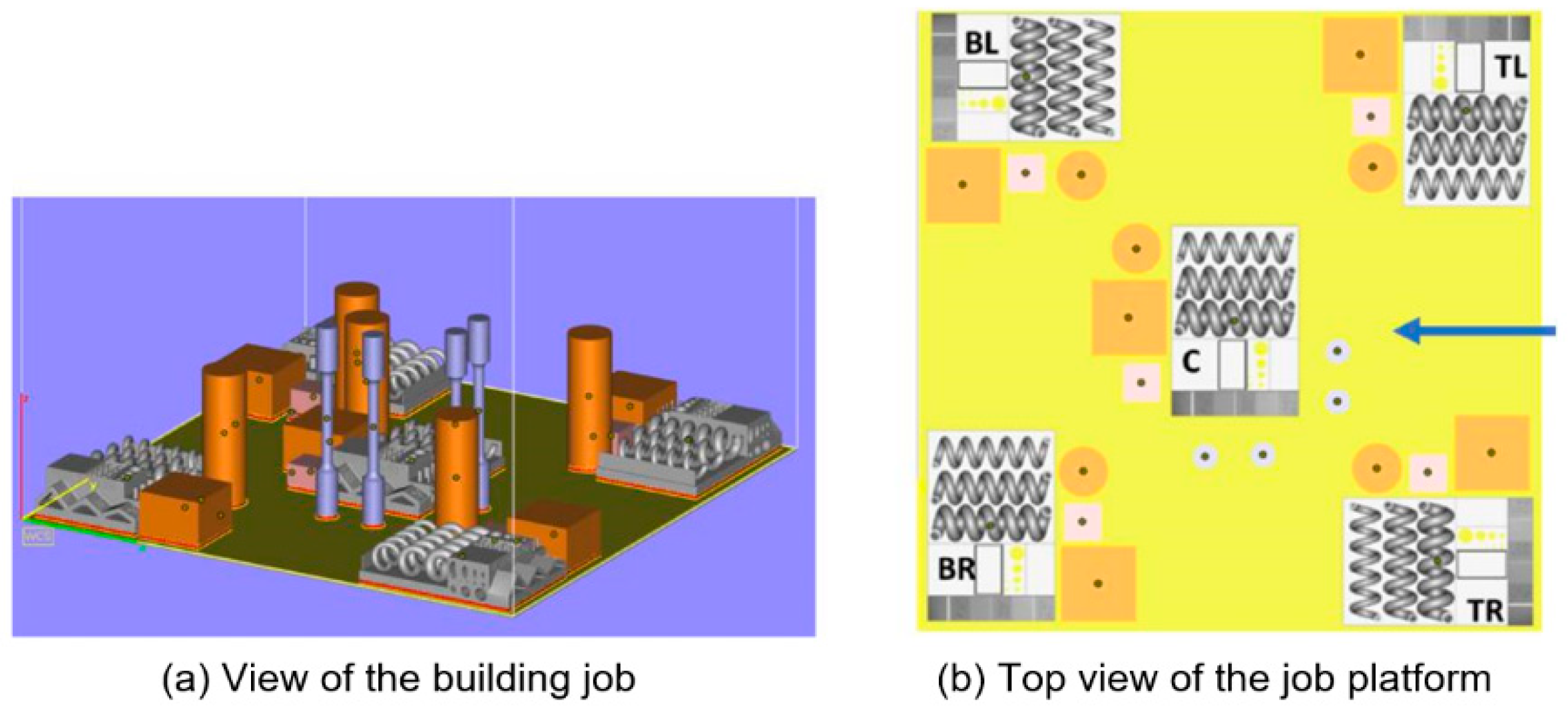
Designing features that have a high probability of failure is critical to highlight the limits of current capabilities of a given technology. Most of the designs in the literature were based on other AM technologies or did not include this “fail test”, where it would not have been possible to easily determine the technological capabilities of using such a design. The design of the complete benchmarking job is presented in Figure 2.
In Figure 2b, the arrow shows the recoating direction, taken as a reference to identify different positions of the samples. Considering the large number of samples involved in the benchmarking, the parts were identified with letters (A, B, C, D, F, G, and H) for the participant, numbers (1, 2, and 3) identifying the job repetition and combinations of letters (BL, BR, C, TL and TR) identifying the position of the sample on the building platform according to the recoating direction (Bottom Left, Bottom Right, Centre, Top Left, and Top Right, respectively).
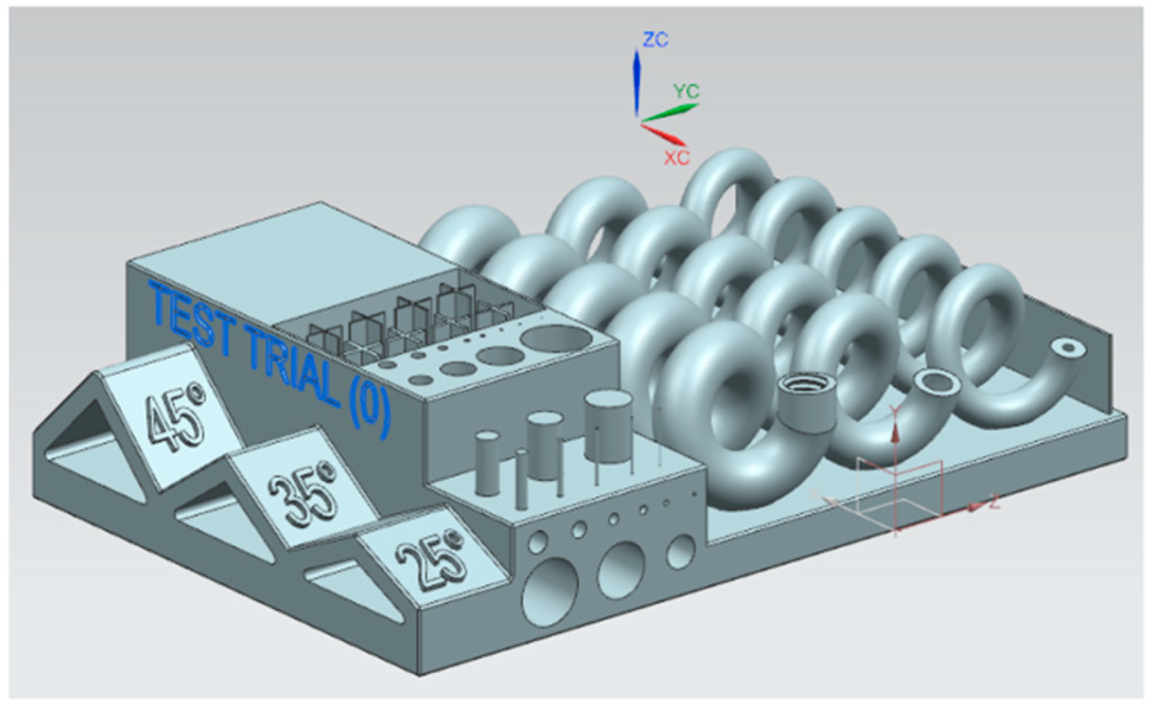
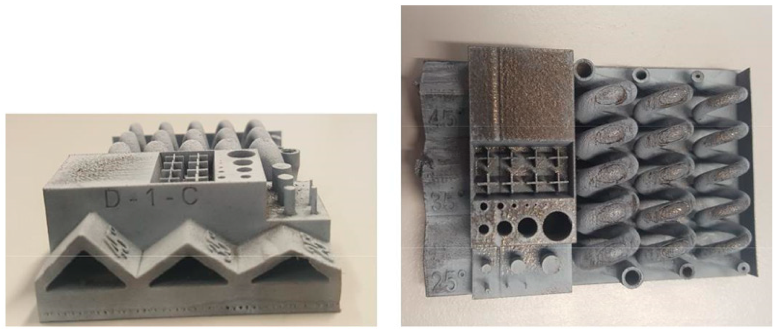
In the spiral samples, it was possible to notice all the features mentioned in Table 3 plus others used for a comprehensive characterization of the machine performance. The sample presented in Figure 3 contains the following features:
- Long thin wall: thickness 0.3 mm; height 7 mm; length 49 mm;
- Eight pins with diameters of 0.1, 0.2, 0.3, 0.5, 1.0, 2.0, 3.0, and 4.0 mm;
- Twelve holes on the top surface with diameters of 0.1, 0.2, 0.3, 0.4, 0.5, 0.8, 1.2, 1.5, 2.0, 3.0, 4.0, and 6.0 mm;
- Eight crosses with wall thicknesses of 0.10, 0.15, 0.20, 0.25, 0.30, 0.35, 0.40, and 0.50 mm;
- Nine holes on vertical surface with diameters of 0.3, 0.5, 0.8, 1.0, 1.5, 2.0, 3.0, 5.0, and 6.0 mm;
- Unsupported pyramids with slopes of 25°, 35°, and 45°;
- Two unsupported spirals with internal diameters of 1.0, 2.5, and 4.5 mm.
The global overview of the samples per job was as follows:
- Five spiral samples;
- Five parallelepipeds with overall dimensions 30 × 30 × 20 mm;
- Five parallelepipeds with overall dimensions 15 × 15 × 10 mm;
- Four tall samples (with the shape of tensile test specimens);
- Five cylinders with diameter 20 mm and height 60 mm.
3. Materials and Methods
Each participant received the STL file for each sample that had to be inserted on the building platform, with an indication of where to place it (see Figure 2b). The choice of sending the STL files directly was made as all of the participants received the designs with exactly the same mesh sizes to avoid having the quality of the products depend on the meshing accuracy. Participants were asked to additively manufacture the parts with new maraging steel powder and not post-process any of the parts, apart from cutting them from the building platform, and to specify the technology used for the separation operation. The companies were informed about the analysis that was going to be conducted and the aspects that were going to be evaluated. Specific aspects of the AM process such as the choice of process parameters and the type of support structures to connect the parts to the platform were left to the companies under the assumption that they were in fact in the best position to understand the equipment and its usage to ensure the best results.
As already mentioned, the material chosen was maraging steel grade 300 (18% Ni Maraging 300, 1.2709), with the chemical composition presented in Table 4.
Then, the analysis of the parts was conducted as follows:
- All spiral samples received (five samples per job for three jobs and seven participants) were coated with a thin layer of TiO2 and measured with a GOM Atos ScanBox 5108 16M 3D scanner. From the results collected, it was possible to evaluate the repeatability among positions and jobs and the distortions of the parts as an indicator of residual stresses. It was also possible, with further analysis of the scan, to determine the deviations of a feature’s dimensions from the nominal CAD design. The data from the scanner were analyzed with GOM Inspect software (as was done, for example, in [23,33]). The authors’ choice of using a contactless system to measure geometrical features (a 3D scanner) instead of more conventional instruments, such as micrometers and calipers, was justified by a preference to obtain more measurement points over an easier and faster measurement technique for more reliable results [34].
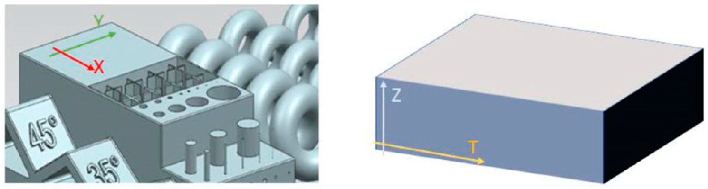
- Figure 4 shows the sample and the direction of the surface roughness measurements: X and Y in the XY Cartesian plane, Z and T in the ZX plane. The surface roughness was measured with a Taylor Hobson Form Talysurf 50 profilometer.
Each measurement was performed only on the central samples for each job. The measurements were conducted according to DIN EN ISO 4288:1998 and 3274:1998. The specifications used are reported in Table 5.
In this report, the choice was to use the Ra parameter for the roughness evaluation, since it is one of the most frequently adopted texture parameters, to allow for an easier comparison of performance in the existing literature [35].
- The homogeneity evaluation was conducted through density measurements on the small parallelepiped (15 × 15 × 10 mm) using the Archimedes principle, as in [36], and by analyzing the residual defects under an optical microscope of two polished surfaces (on the XY and ZX planes) of all central big parallelepipeds (30 × 30 × 20 mm). The samples were mirror-polished on the two surfaces and observed under an optical microscope, and the pictures collected were elaborated with ImageJ software, as in [37]. The images were converted to black and white to count the number of darker pixels that were considered residual defects by using a specific tool in the software. In many industrial applications, the surface of LPBF products needs to be post-processed, in particular polished, to obtain the required surface quality. When defects are presented close to the surface, for example, residual porosities or inclusions, the surface quality after polishing will not be acceptable, and this is why it was important to evaluate this aspect.
- Rockwell C (HRC) was the method chosen for hardness evaluation, as in [38], and it was performed on a clean surface, slightly ground, in the XY and ZX planes.
- Moreover, the time necessary for producing each job was recorded and compared. As already mentioned, all but one of the machines were among the newest technology on the market, and in this paper are identified with letters. Table 6 shows the shareable information from the participants (i.e., type of company, number of lasers, technology used to separate the parts from the building platform, and layer thickness used for production).
Company E was not able to produce three complete jobs, so no results from E are presented in this research.
4. Results
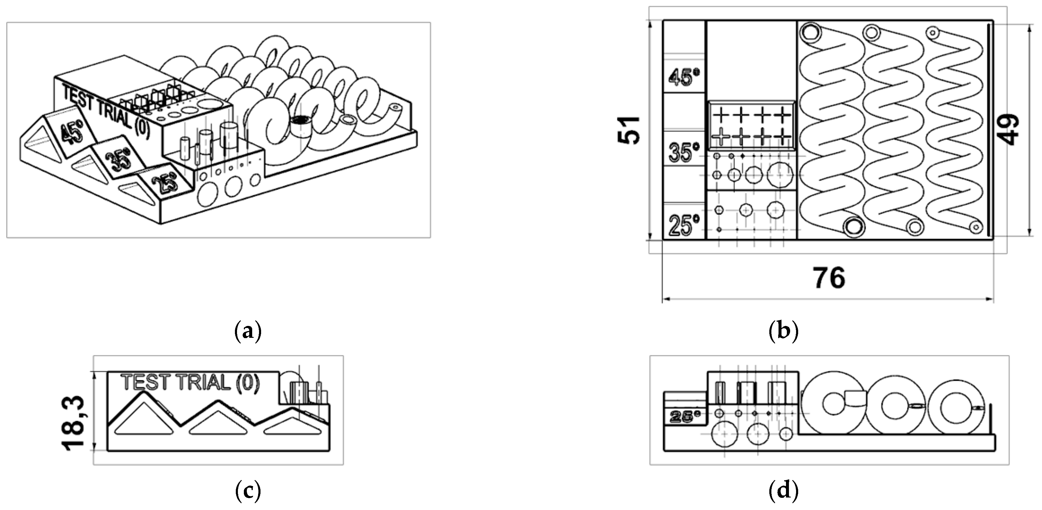
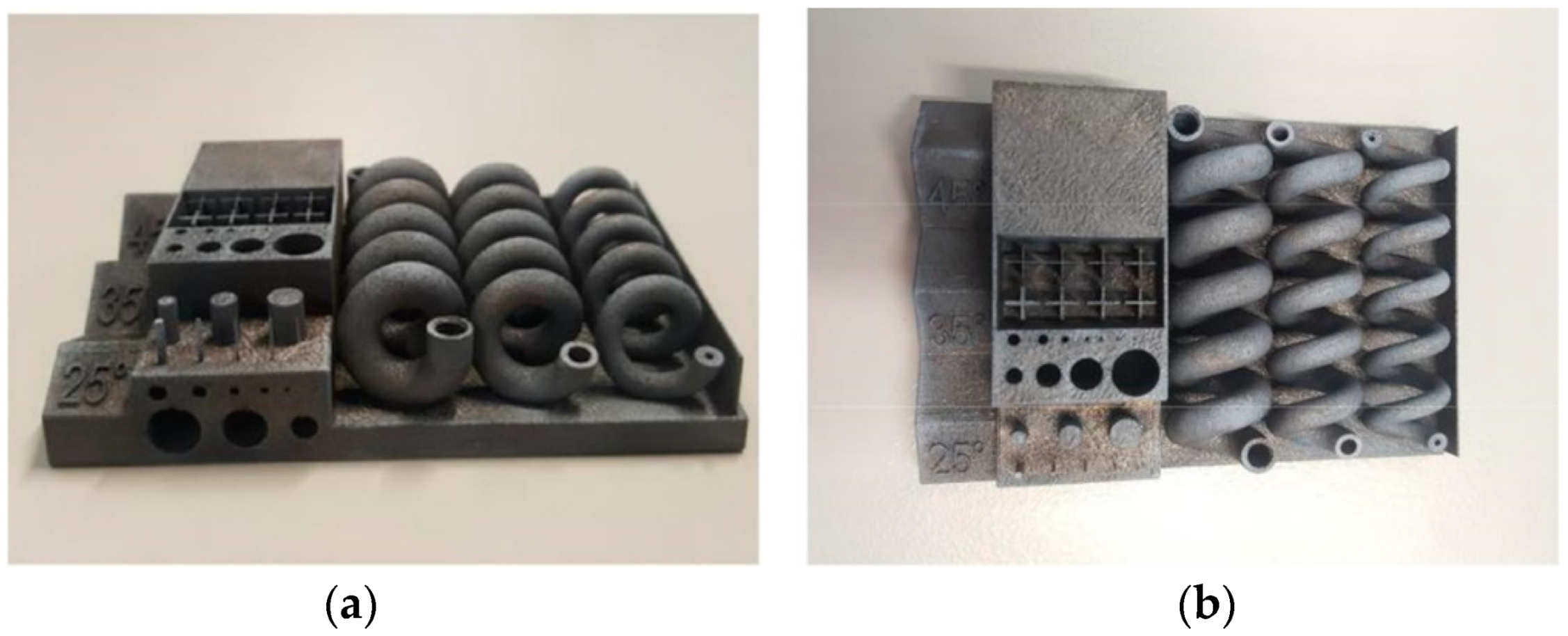
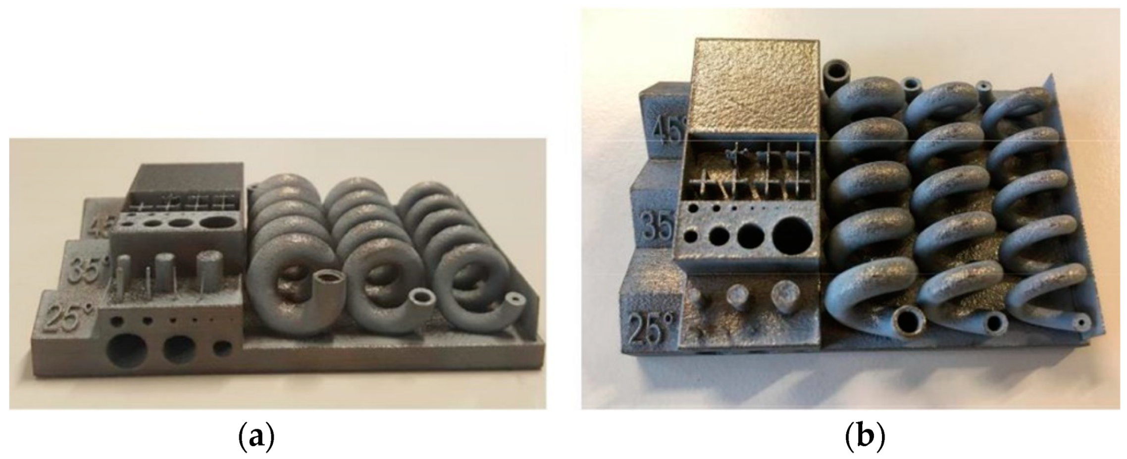
In this section, all the results collected from the above-mentioned analysis are presented. Figure 5 shows the CAD drawing of the part with reference dimensions, and Figure 6 and Figure 7 show some of the manufactured samples.
The white residuals on the surface of some parts came from the TiO2 coating used for the 3D scanning of the parts. Examining the parts when they were still attached to the building platform, it was possible to do some useful observation such as in Figure 8, where a significant part distortion that generated delamination of the parts from the platform can be seen.
Another aspect immediately visible from the pictures is the effect of the choice of tool to cut the part from the building platform. We noticed that the use of a wire-cut electrical discharge machining (EDM) left the bottom surface smoother and more precise, with the risk that rust would be created on the surface if a water dielectric was chosen, as happened for some participants.
4.1. 3D Scanner Results: Accuracy, Repeatability, and Complex Feature Production
All the results generated by the 3D scanner of the spiral samples were produced by using Gaussian best fit alignment, focusing on three surfaces to obtain a more comprehensive and robust comparison of the dimensions and distortions of parts. The first two surfaces used for the alignment are presented in Figure 9.
An additional surface for alignment, focusing on the thin wall of the spiral sample, was used to more accurately evaluate the distortion of the part, as presented in Figure 10.
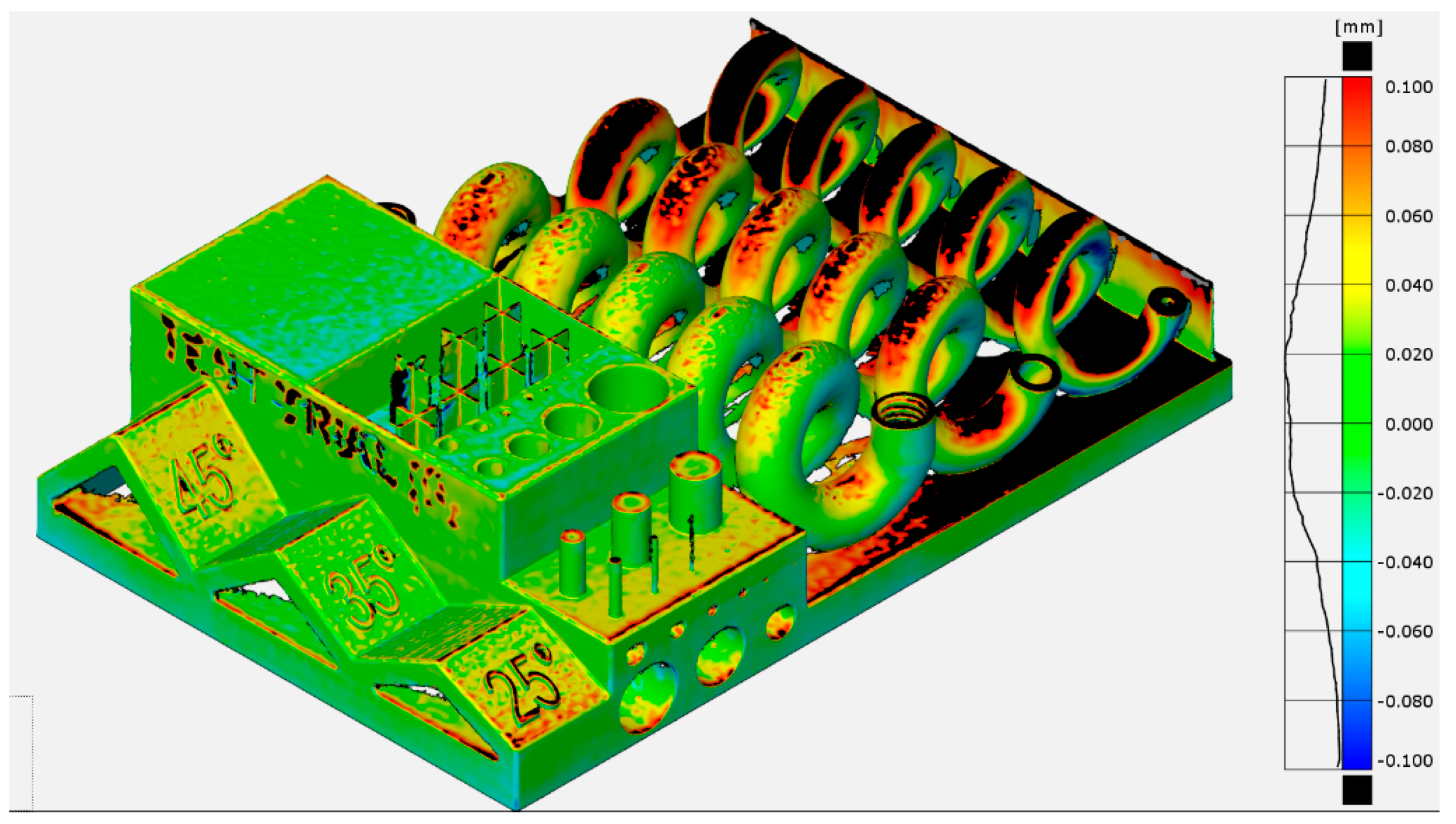
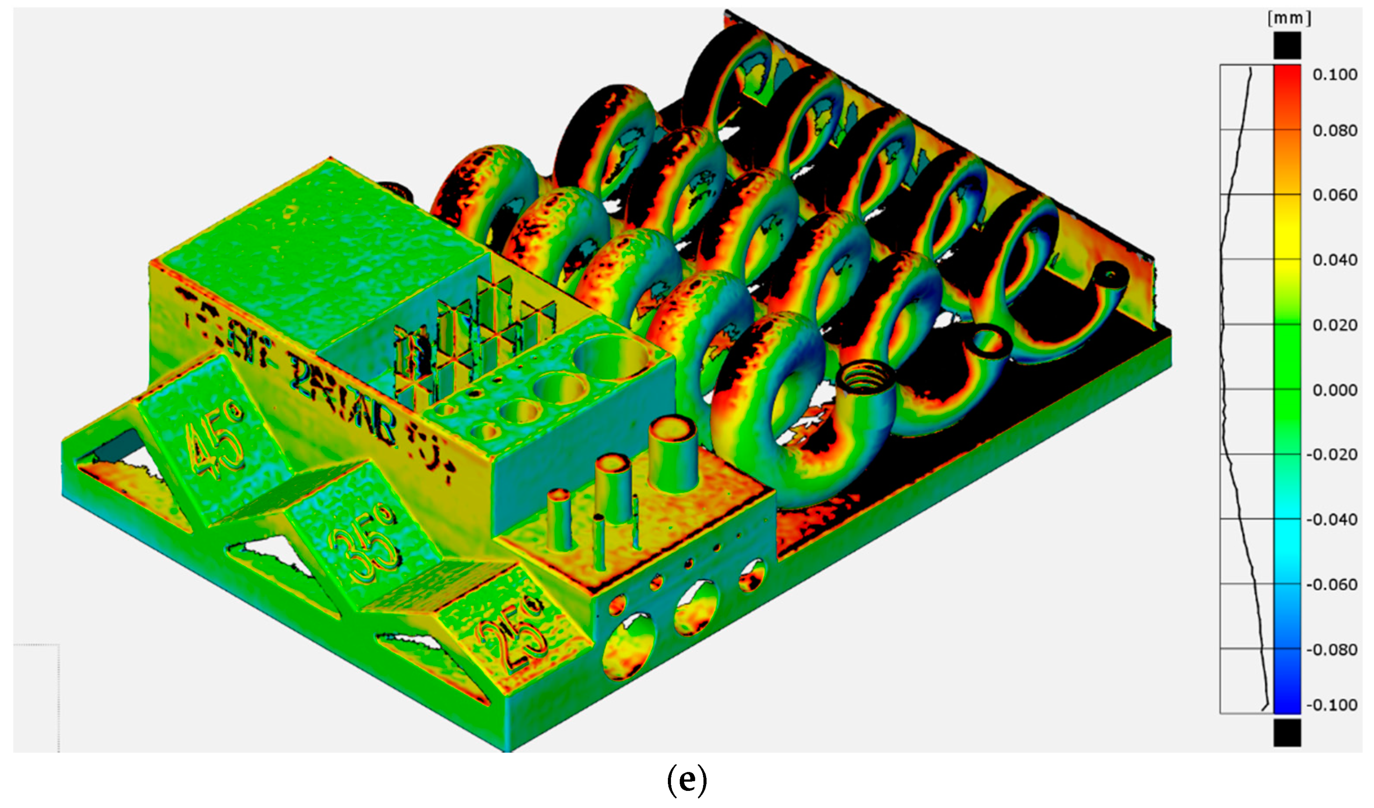
An example of a color plot generated from the 3D scanner is given in Figure 11.
On the right side of the color plot, the scale bar shows the upper and lower limits, chosen as +/− 0.1 mm, since greater distortions would make the part unacceptable for most applications.
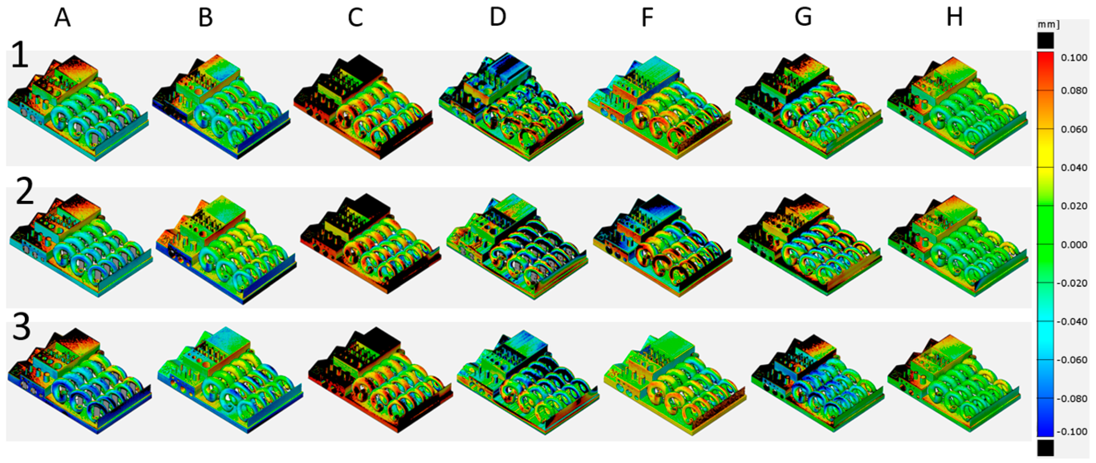
The generated color plot was used to evaluate the repeatability of the machines across jobs and positions. A comparison of the color plots between different suppliers across the jobs for each company is shown in Figure 12 for all central positions.
It is evident in Figure 12 that repeatability across jobs is not ensured for all machines, for example, in the color plots for participants A, B, D, F, and G, where the deviations differed for all three jobs. In addition, repeatability was not ensured across different positions, as presented in Figure 13 for company G.
Figure 14 shows an example of a high repeatable job from company H.
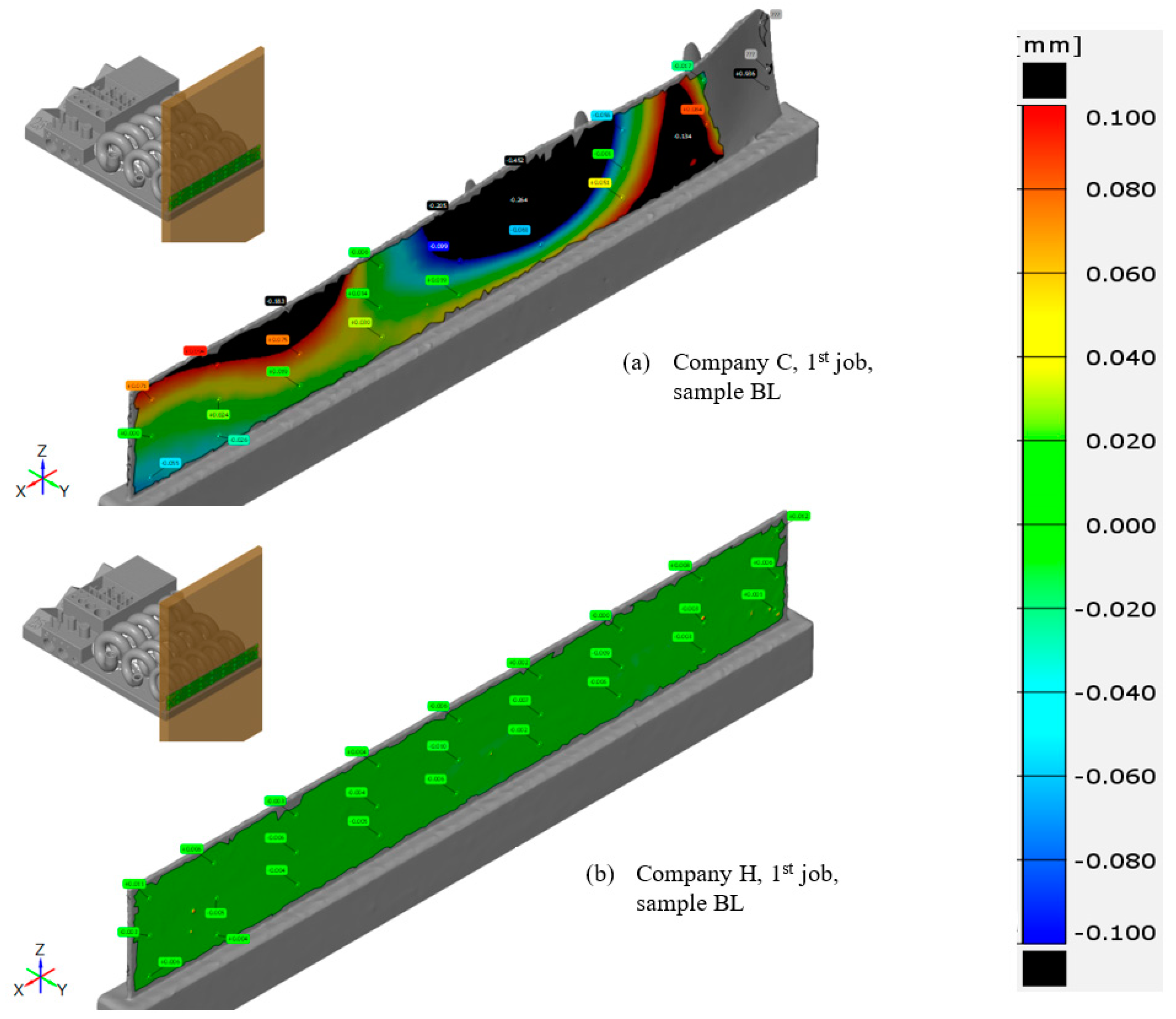
Considering the same printing job, the dimensional analysis highlights that the parts produced were affected by some repeatability issues depending on their position on the building platform. Similar observations could be made for all participants. A distortion evaluation was conducted by looking at the entire color plot (and for some companies these were particularly evident such as for company C in Figure 12) as well as by comparing the distortions, focusing on the deviations of thin walls compared to the nominal design. A comparison is presented in Figure 15.
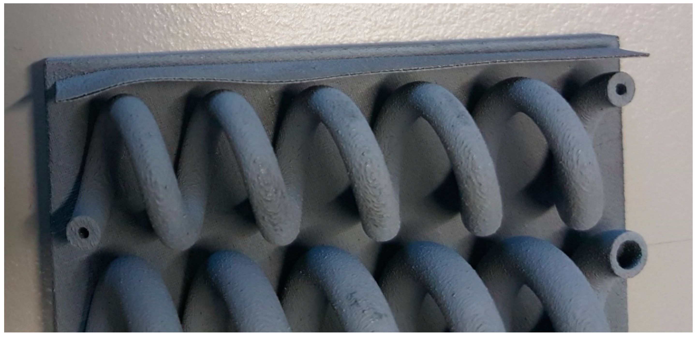
For some companies such as C, distortions on the thin walls were extremely evident and already visible during the visual inspection, as shown in Figure 16.
From the 3D scanner results, all features were analyzed to evaluate how much they deviated from the nominal CAD design. The first objective of features such as pins and crosses is to immediately understand whether the machine is capable of producing them or not, as a pass/fail evaluation. In the following tables, the pass/fail test results are presented for each supplier and for all pins and crosses.
Starting from the pin’s features, Table 7 shows which features managed to be produced and which did not. The analysis and dimensions were assessed with an optical microscope. The number of features is in the same ascending order as in Section 2, here reported again: diameter of pins 1–8: 0.1 mm, 0.2 mm, 0.3 mm, 0.5 mm, 1 mm, 2 mm, 3 mm, and 4 mm. The symbol legend is as follows: ✓ acceptable; ≈ uncertain; ✗ not built. A feature was considered acceptable when it was fully built, with approximately the dimensions defined in the CAD that could be measured with the optical microscope, also tolerating slightly bent pins because of normal handling. A feature was considered uncertain when it was properly built but too bent to be measured, in order to confirm its dimension compared to the nominal.
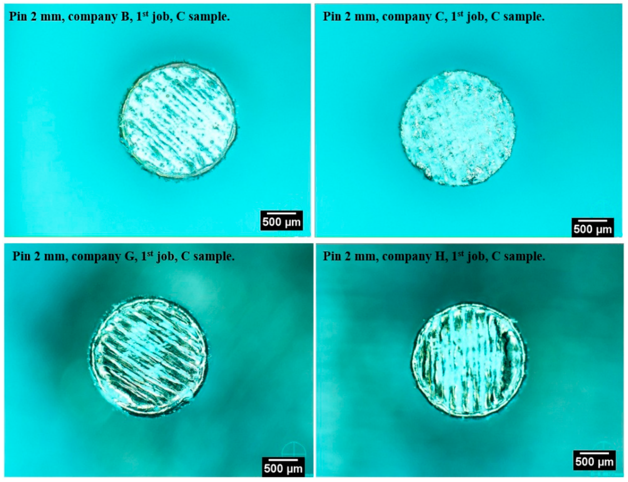
The optical microscope analysis revealed that most of the smallest pins (i.e., 0.3 mm diameter or less) were deformed or completely bent. As far as the largest pins were concerned, it was possible to distinguish the contour lie from the internal filling of the laser scan track, as presented in Figure 17.
With GOM Inspect analytical software from the 3D scanner, the deviation of dimensions of the printed features compared to the nominal design was plotted, and shown in Figure 18. In the graph, the samples are defined on the x-axis, and the y-axis shows the deviation from the nominal CAD design (referred as 0). Each line color represents a different pin, while each peak/valley is a different sample. On the top, the companies are indicated for each region of the graph.
Some of the lines of the deviation graph look interrupted or completely out of average; this is again due to the fact that most of the smallest pins were broken or bent (probably due also in part to handling), and therefore it was not possible to obtain a proper measurement. It is interesting to observe that most of the companies produced pins that were smaller than the nominal CAD dimension.
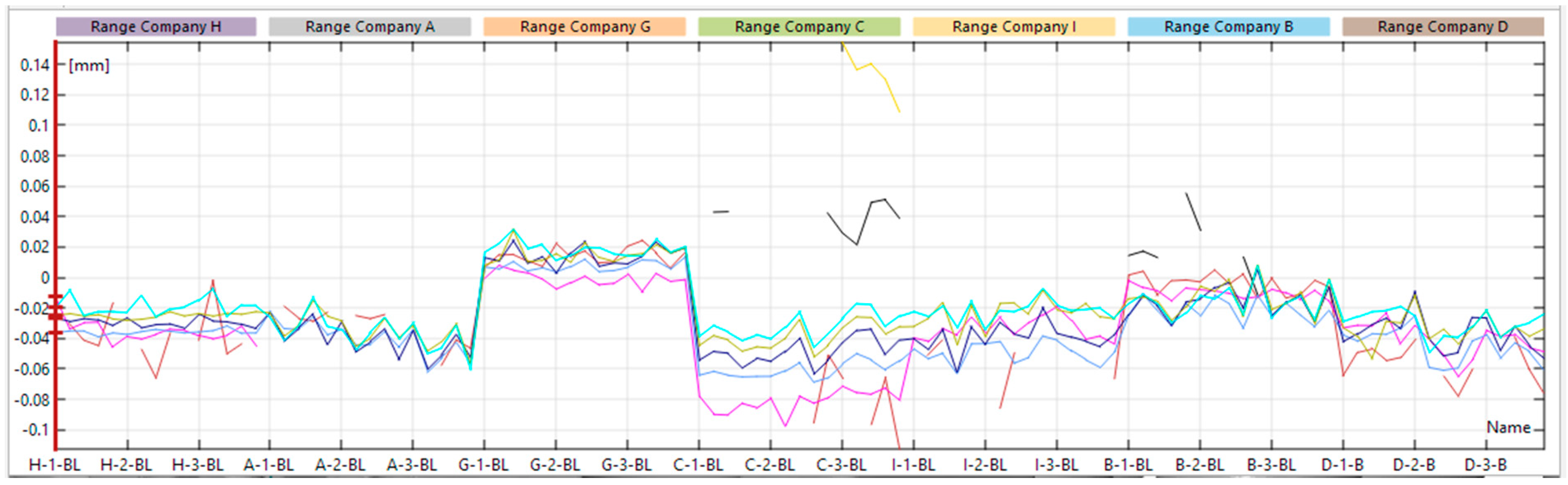
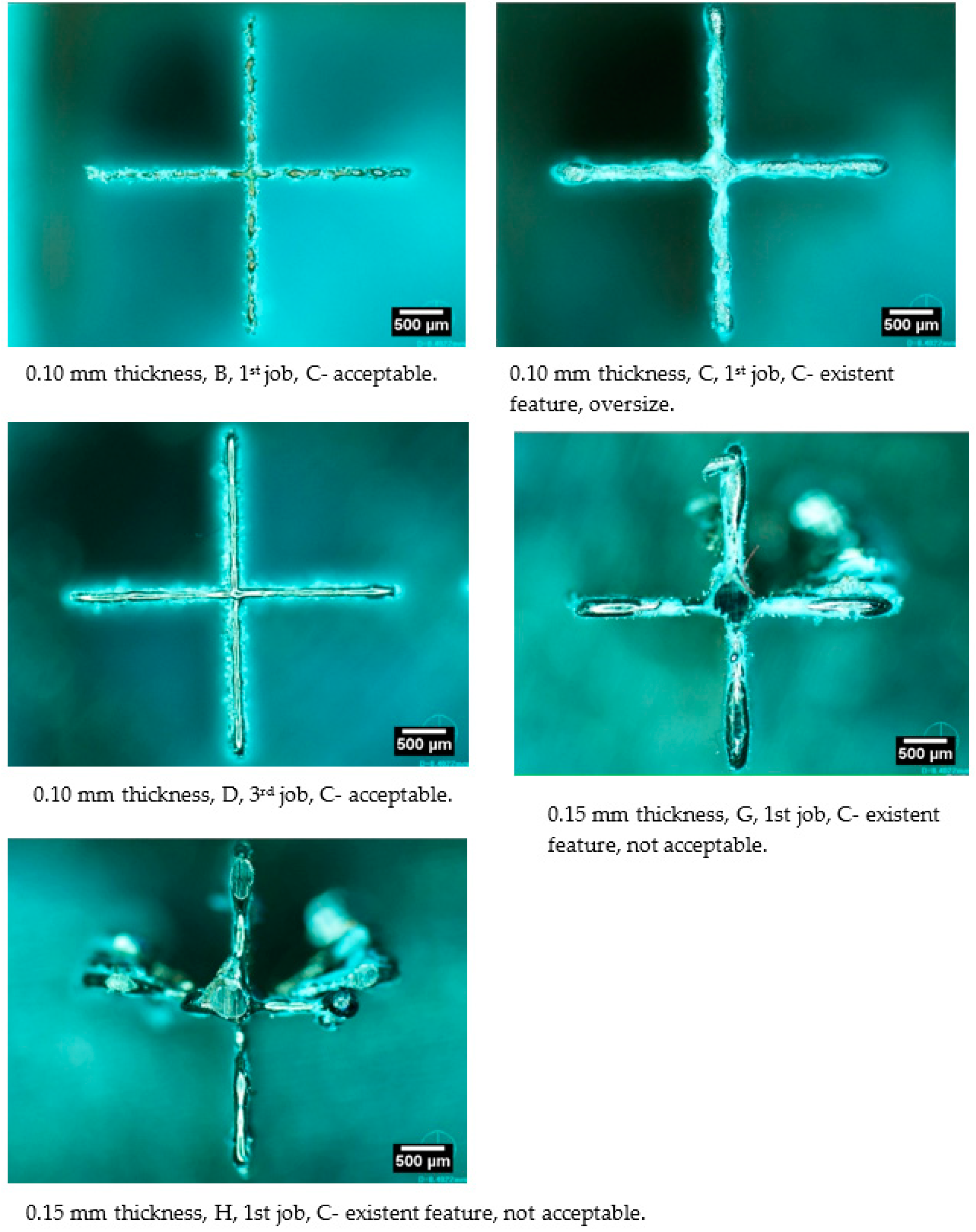
The same investigation was conducted for the crosses, and Table 8 shows a summary of the pass/fail dimensions. Crosses 1–8 had the following dimensions (vertical and horizontal wall thickness): 0.10 mm, 0.15 mm, 0.20 mm, 0.25 mm, 0.30 mm, 0.35 mm, 0.40 mm, and 0.50 mm, respectively. The symbol legend is as follows: ✓ acceptable; ≈ existing feature, oversize; ✓ existing feature, not acceptable; ✗ not built.
Measurement of the crosses was carried out with an optical microscope and a 3D scanner. Some pictures collected with the optical microscope are presented in Figure 19, and also show the shapes of the crosses that were considered to be not acceptable.
Again, the deviation analysis of the real dimensions of the features against the nominals from the GOM software is reported in Figure 20.
One reason why most of the crosses of small dimensions, compared to the pins, were built while the pins were not is due to the geometry of the features. The pins, whose dimensions were almost as large as the beam focus (around 80 μm for most of the suppliers), were built with a single laser shot, while the crosses were made of an entire scan track, which is inherently more resistant, for a more robust design.
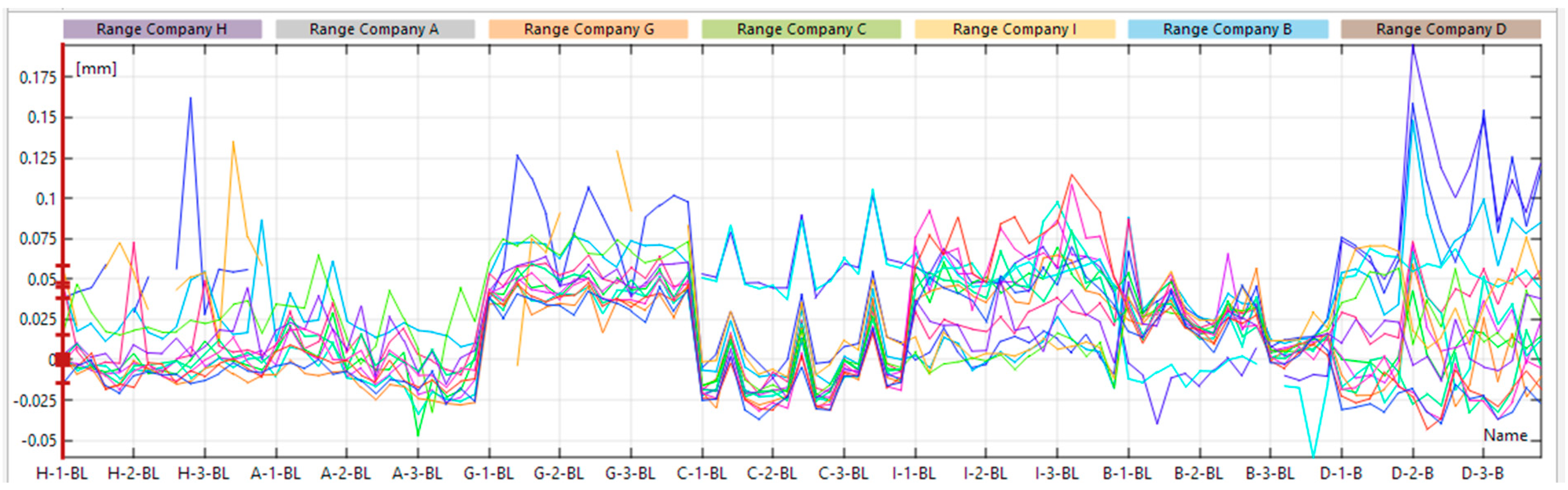
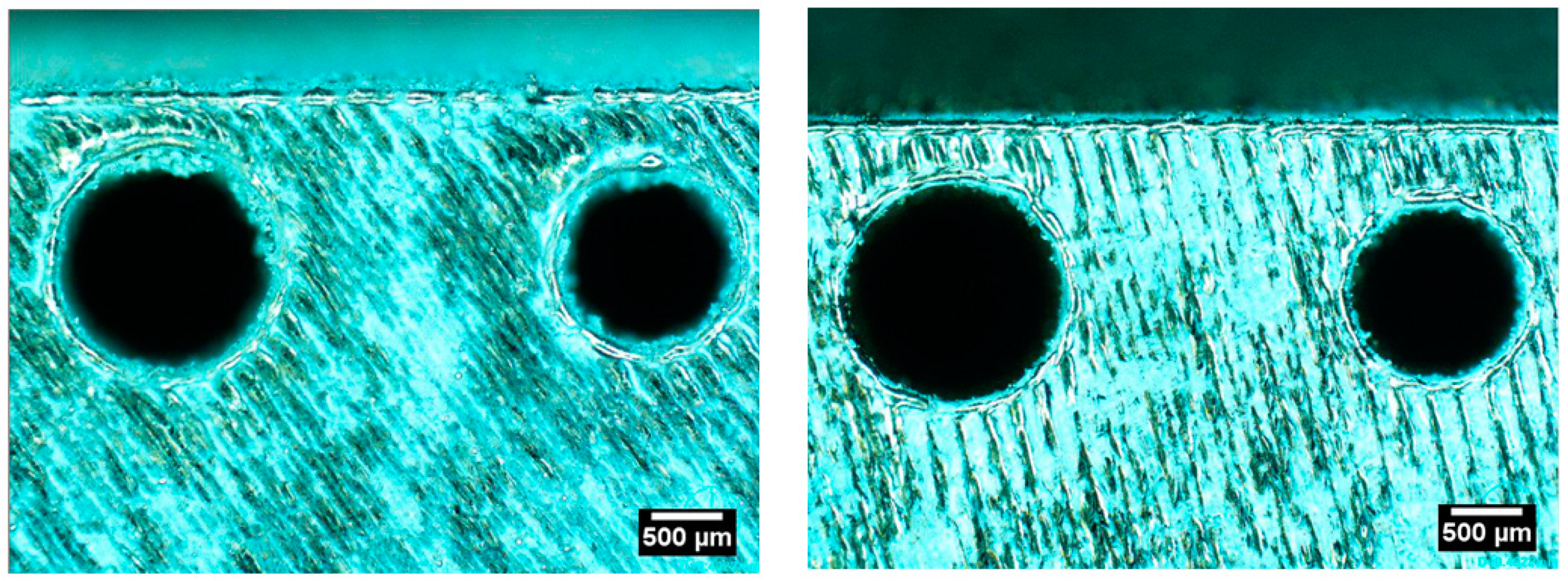
The same type of evaluation was conducted for the holes, in particular using the deviation analysis produced by the GOM software. The deviation graph of the real dimensions compared to the nominal dimensions is plotted in Figure 21.
Examples of holes are given in Figure 22.
Observing and comparing the deviation graphs of the average diameters of pins and holes, it is possible to consider the beam offset. As reported by Moylan et al., a too large beam offset can be recognized when the diameters of the pins are smaller than the nominal, while the holes are larger. On the contrary, a too small beam offset generates larger pins and smaller holes than the nominal [14]. This tendency can be recognized for company C, for which the beam offset was too large, and to some extent for company G, which had a too small beam offset.
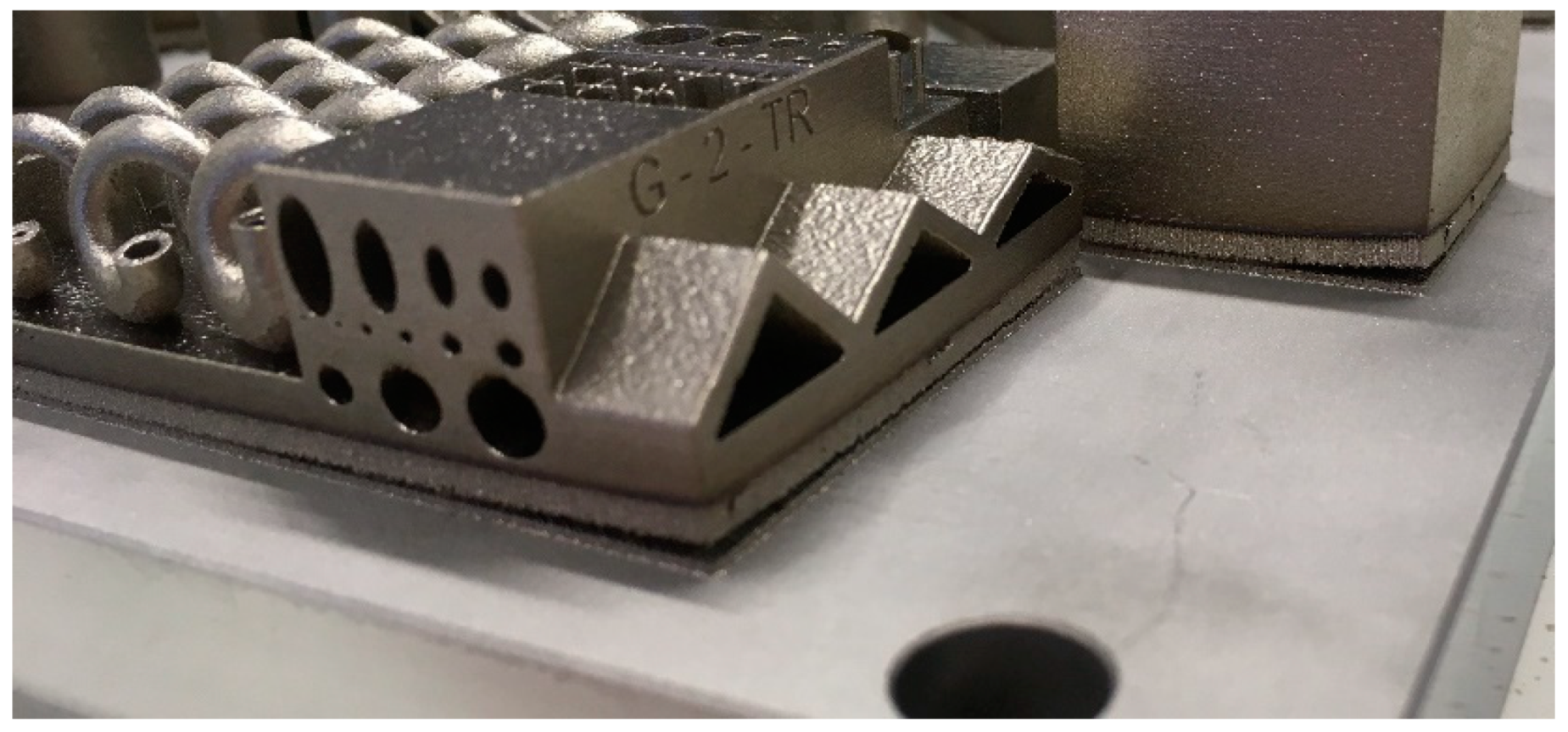
The last important feature that needs to be considered in this evaluation is unsupported pyramids (see Figure 23).
All the companies managed to produce a pyramid, even ones most inclined at 25°, for all positions and jobs. Only one of the participants, D, presented some issues with the down-facing surface, most likely due to the wrong choice of process parameters for this type of surface, particularly critical in LPBF, and/or damage on the recoated surface that is also visible on the top. Figure 24 shows the pyramids and recoated issues.
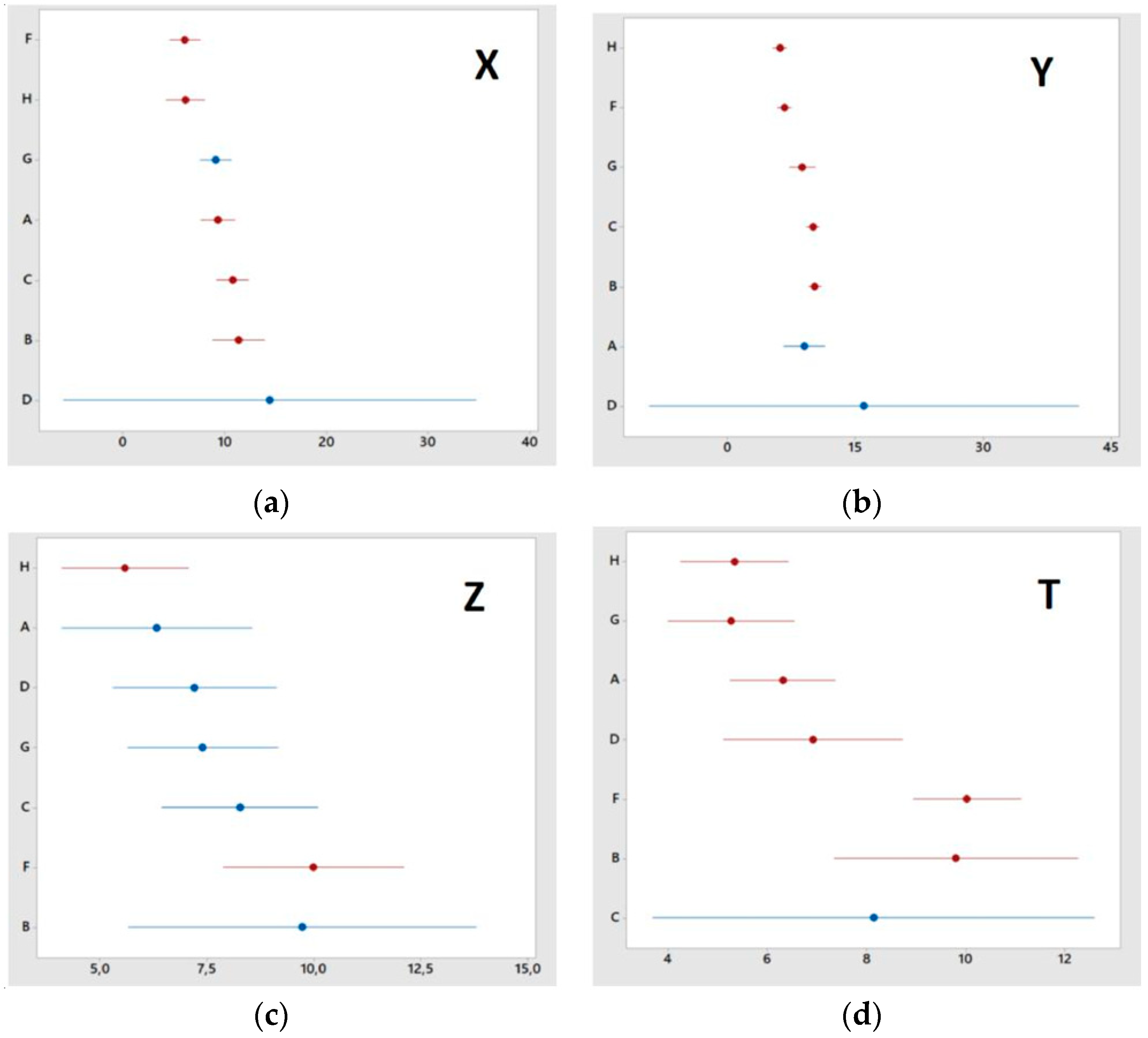
4.2. Surface Roughness: Accuracy
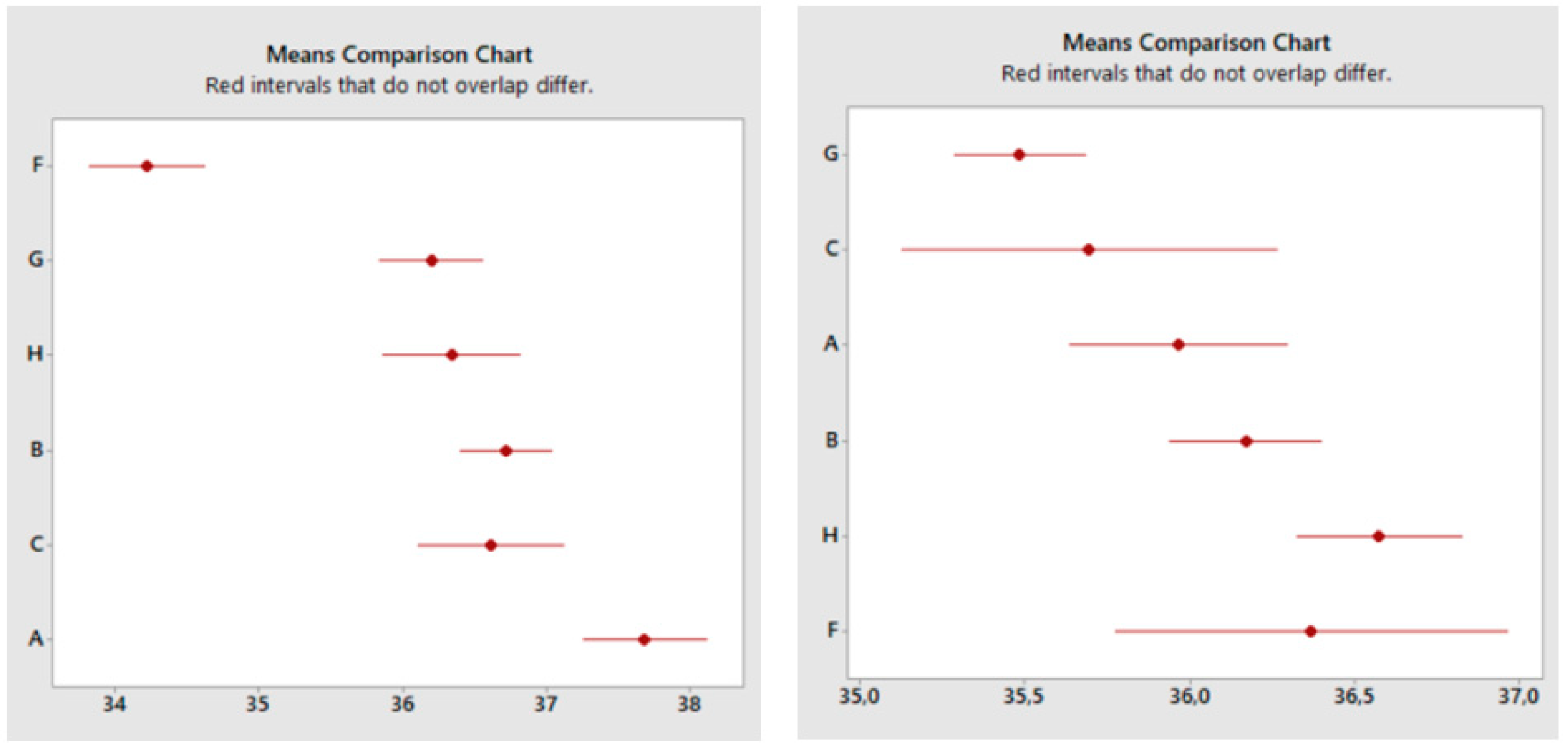
The surface roughness was evaluated in four directions (Figure 4), using the Ra parameter and repeating each measurement at least three times. Table 9 shows the collection of results, showing the company, direction, average (avg, in μm), and standard deviation (std.-dev).
All the data presented were analyzed using Minitab software with one-way ANOVA to recognize particular trends depending on the job number for each direction. For companies A, F, and H, there were no significant differences among jobs for any direction; all of the other companies revealed some discontinuities. To summarize, Figure 25 shows the means comparison charts from the one-way ANOVA analysis for all directions.
4.3. Homogeneity
The homogeneity of the products was evaluated both by analyzing the density and by measuring the quantity of residual defects after polishing two sides (XY and ZX planes) of the cubes. The density results are presented in Table 10, and relative density was calculated as follows:
where the theoretical bulk density was considered to be 8.1 g/cm3, as mentioned in Section 3.
As expected, density for most of the participants was above 99%, except for company D, again most likely because of the recoated issue that did not ensure proper distribution of the powder.
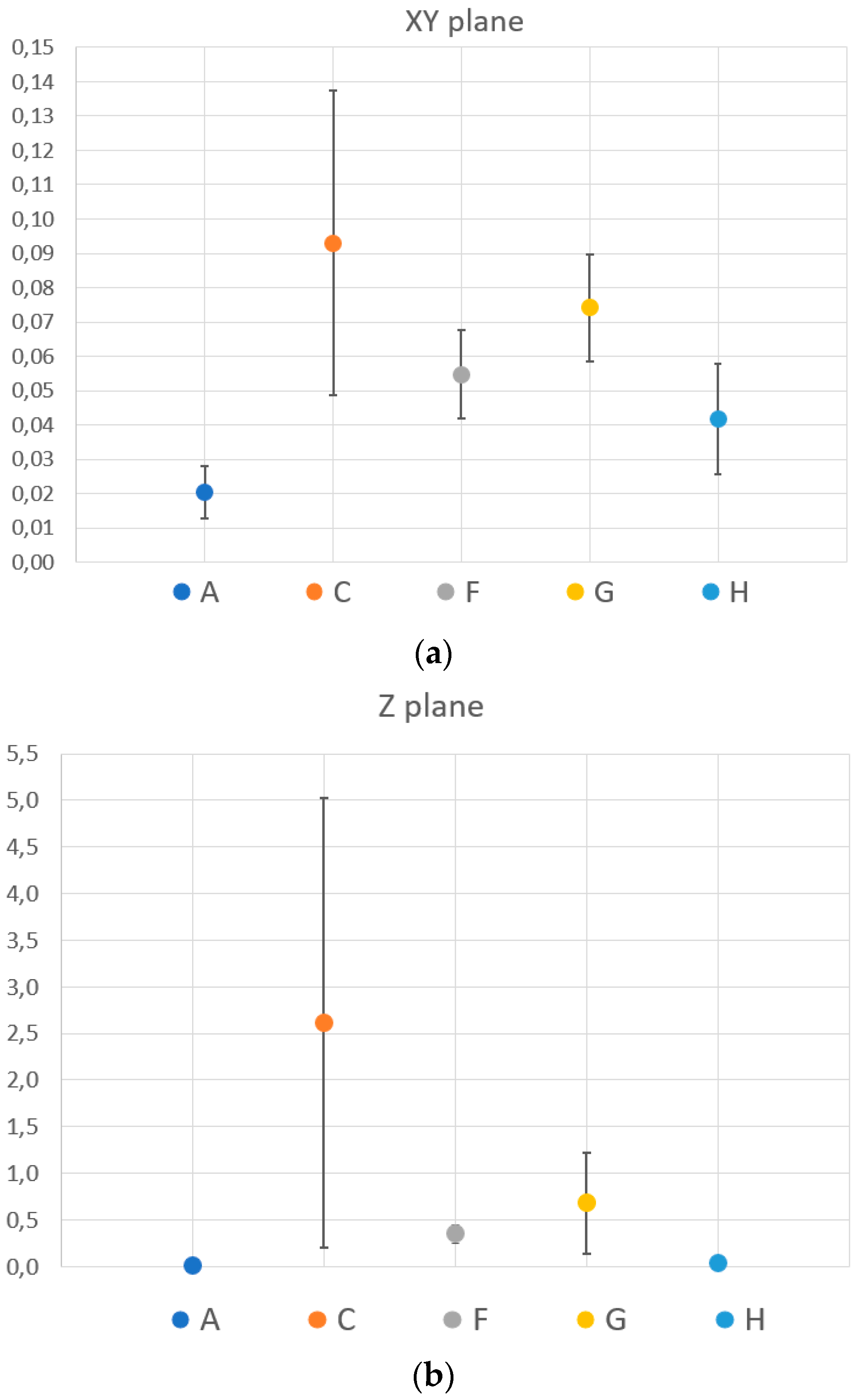
For evaluation of the residual defect, the central larger parallelepiped was polished on two surfaces: XY (parallel to the building platform) and XZ (one of the growing sides). Using ImageJ software, as in [30], the number of defects was calculated to produce the results presented in Table 11 and plotted in Figure 26. The defects identified with this method were recognized as residual porosities or inclusions in the material.
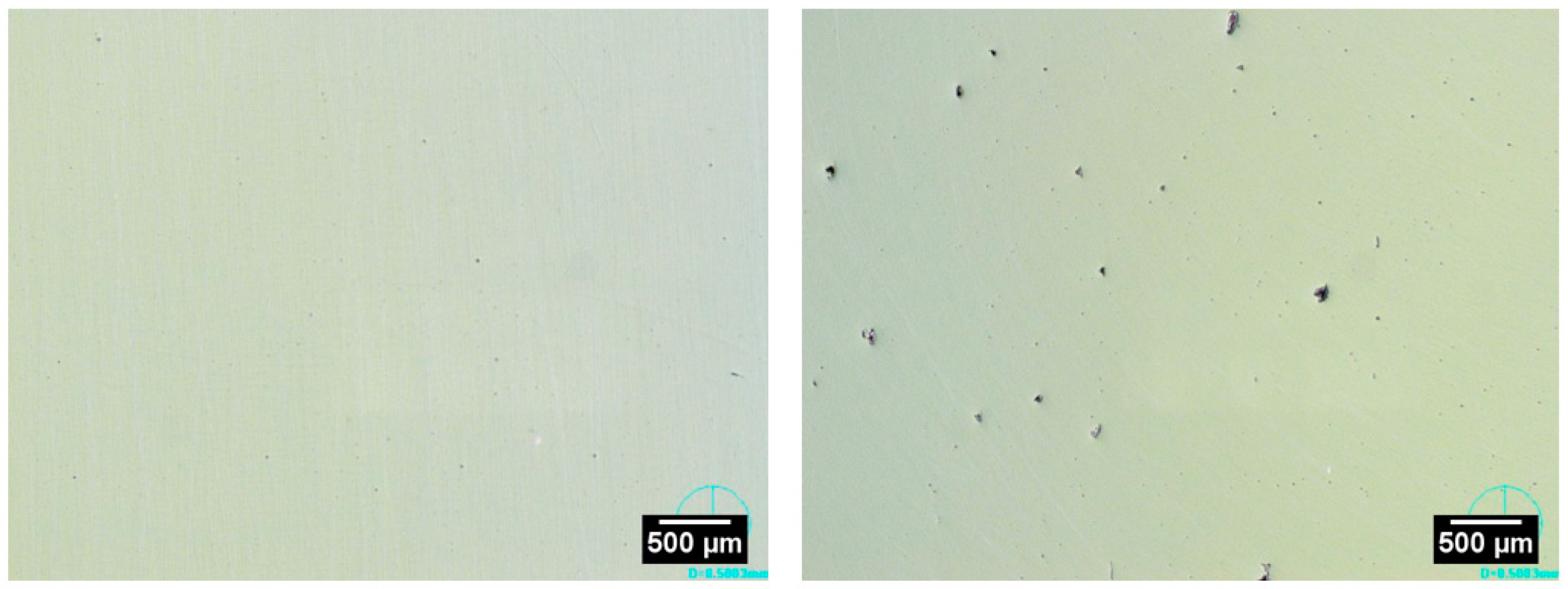
The participant that showed the highest percentage of residual defects on the surfaces was C (see Figure 27, showing two selected pictures for each face).
The sample from company C presented multiple defects in some areas of the XZ surfaces of dimensions considerably bigger than all samples from other companies or from the same company, but on the XY face, which explains the very big deviations of values seen in Figure 26. To precisely define the source of these differences, further analysis would be required.
4.4. Mechanical Properties: Rockwell Hardness C
Rockwell hardness C (HRC) was measured for two sides, XY and XZ, on the as-built parts. The means charts are presented in Figure 28.
As expected, no relevant differences were recorded from the conventional value of HRC for non-heat-treated maraging steel grade 300 [39]. One-way ANOVA analysis was conducted to identify eventual variation across jobs and positions, but it was negligible.
4.5. Build Speed Comparison
The average time required to print each job was provided by the participants to have a reference for the building speed of the machine. Table 12 reports the times along with the number of lasers that the specific machine used for the job.
It is clear that the build time was influenced mainly by the number of lasers and not by how new the machine was. Other factors that certainly influenced the build time are related to the process parameters chosen and the scan strategy.
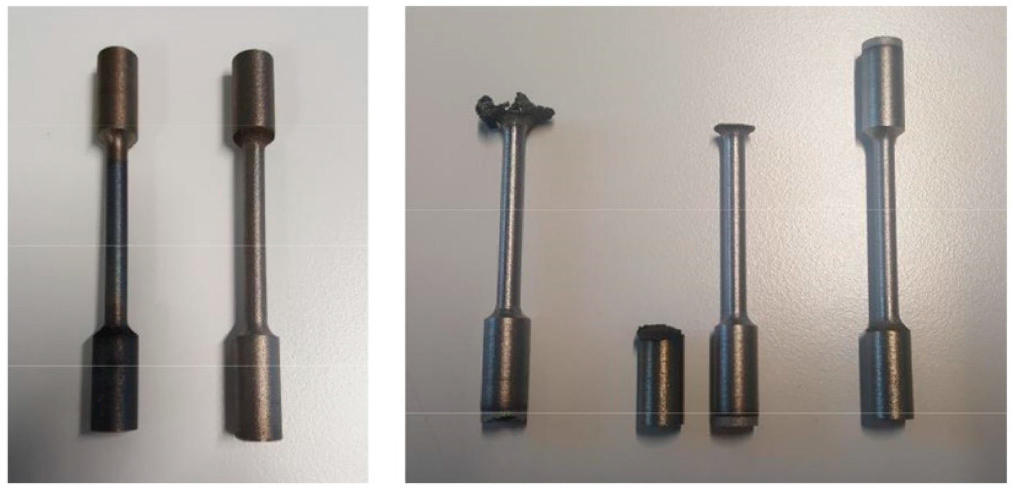
4.6. Tall Parts Production
Tall specimens with the shape of tensile test samples were used to evaluate the capability of the machines to build relatively tall parts (more than 80 mm, with a 10 mm base diameter). Figure 29 shows selected pictures.
Apart from company G, all participants managed to produce most of the samples.
5. Discussion and Conclusions
In this work, the authors present the results from an extensive benchmarking activity conducted on LPBF machines, comparing the performance of five state-of-the-art machines operated by their respective manufacturers and two-state-of-the art machines operated by their respective owners (end users), and contrasting the newest machine capabilities with a machine more than 10 years old. The old machine, identified with the letter H, was an EOS M270. Table 13 presents an overview of the results collected with related discussion.
The outcomes of the benchmarking work can be summarized as follows:
- Considering the good results from company H, which used the oldest machine, it is evident that user experience and expertise play large roles in the final quality of the delivered product.
- The part design presented for realizing holistic benchmarking of LPBF machines was successful in achieving the goal.
- According to this work, even the newest machines did not outperform the older machine.
- One of the major trends revealed by analyzing the newest systems is the focus of machine manufacturers on building larger and faster machines; this goal is currently achieved in the industry by increasing the number of lasers, but little attention is given to other factors (such as higher repeatability and the ability to print tiny features, or improving the surface roughness), as was observed during this work.
LPBF, and AM in general, is technology that is trying to overcome prototyping applications to create its own space in industrial production. In order to help this technology achieve this ambitious goal, it is extremely important that the process become more robust, in terms of better repeatability and less dependence on the user’s experience.
An additional consideration of this work can be made regarding the suitability of using a benchmarking component to compare different AM technologies, particularly considering the multiple attempts made in recent years to standardize a design for additive manufacturing. Given the seven categories of AM technology, even if they all essentially build parts layer upon layer, they are profoundly different from each other with respect to the basic working principles and the materials they consider (for example, in PBF, both metal and polymer powders can be processed), so it is very complex, if not impossible, to create a unique design without considering the final application of products built with the technology. Moreover, considering the fast development of all AM technologies, specific geometrical aspects such as the minimum feature size (both external and internal) and the components’ overall size should always be updated. As a final reflection on how this work integrates in the landscape of previous benchmarking research for AM, it is the first attempt to evaluate the influence of the specific machine used, by multiple manufacturers, from a holistic perspective, requiring the design of not only a single artifact but a complete job that integrates designs for metrology concepts to ensure the measurability of all specimens and features.
Author Contributions
Conceptualization, M.M., S.M. and G.T.; methodology, M.M.; validation, M.M. and S.C. (Stefano Candeo); formal analysis, M.M. and S.C. (Stefano Candeo); investigation, M.M. and S.C. (Stefano Candeo); resources, M.M.; data curation, M.M. and S.C. (Stefano Candeo); writing—original draft preparation, M.M.; writing—review and editing, M.M., S.M. and G.T.; visualization, M.M. and S.C. (Stefano Candeo); supervision, M.M., S.C. (Simone Carmignato), S.M. and G.T.; project administration, M.M.
Funding
The project received funding from the European Union’s Horizon 2020 Marie Sklodowska-Curie grant agreement No. 721383, for the Precision Additive Metal Manufacturing (PAM2) project.
Acknowledgments
The authors are grateful to all the companies that took part in this benchmarking study, and who provided samples and information and helped to define the current status and future perspectives of LPBF technologies. The authors also thank Sven Dalager Sørensen, Peter Noes Poulsen, André Larsen, Ronen Hadar, and Christian Wissing Kruse.
Conflicts of Interest
The authors declare no conflicts of interest.
References
- Gibson, I.; Rosen, D.W.; Stucker, B. Additive Manufacturing Technologies, 2nd ed.; Springer: New York, NY, USA, 2015. [Google Scholar] [CrossRef]
- Hopkinson, N.; Hague, R.J.M.; Dickens, P.M. Rapid Manufacturing. In An Industrial Revolution for the Digital Age; John Wiley & Sons, Ltd.: Hoboken, NJ, USA, 2006. [Google Scholar] [CrossRef]
- Conner, B.P.; Manogharan, G.P.; Martof, A.N.; Rodomsky, L.M.; Rodomsky, C.M.; Jordan, D.C.; Limperos, J.W. Making sense of 3-D printing: Creating a map of additive manufacturing products and services. Addit. Manuf. 2014, 1, 64–76. [Google Scholar] [CrossRef]
- Quinlan, H.E.; Hasan, T.; Jaddou, J.; Hart, A.J. Industrial and Consumer Uses of Additive Manufacturing: A Discussion of Capabilities, Trajectories, and Challenges. J. Ind. Ecol. 2017, 21, S15–S20. [Google Scholar] [CrossRef] [Green Version]
- ASTM International. F2792-12a—Standard Terminology for Additive Manufacturing Technologies. Rapid Manuf. Assoc. 2013, 10–12. [Google Scholar] [CrossRef]
- Huang, Y.; Leu, M.C.; Mazumder, J.; Donmez, A. Additive Manufacturing: Current State, Future Potential, Gaps and Needs, and Recommendations. J. Manuf. Sci. Eng. 2015, 137, 14001. [Google Scholar] [CrossRef] [Green Version]
- Gu, D.D.; Meiners, W.; Wissenbach, K.; Poprawe, R. Laser additive manufacturing of metallic components: Materials, processes and mechanisms. Int. Mater. Rev. 2012, 57, 133–164. [Google Scholar] [CrossRef]
- Gu, D. Laser Additive Manufacturing of High-Performance Materials; Springer: Berlin/Heidelberg, Germany, 2015. [Google Scholar] [CrossRef]
- Frazier, W.E. Metal additive manufacturing: A review. J. Mater. Eng. Perform. 2014, 23, 1917–1928. [Google Scholar] [CrossRef]
- Herzog, D.; Seyda, V.; Wycisk, E.; Emmelmann, C. Additive manufacturing of metals. Acta Mater. 2016, 117, 371–392. [Google Scholar] [CrossRef]
- Mahesh, M.; Wong, Y.S.; Fuh, Y.H.; Loh, H.T. Rapid prototyping and manufacturing benchmarking. Sofwtare Solut. RP 2002, 1, 57–94. [Google Scholar]
- Mahesh, M.; Fuh, J.Y.H.; Wong, Y.S.; Loh, H.T. Benchmarking for decision making in rapid prototyping systems. In Proceedings of the IEEE International Conference on Automation Science and Engineering, Edmonton, AB, Canada, 1–2 August 2005; pp. 19–24. [Google Scholar] [CrossRef]
- Rebaioli, L.; Fassi, I. A review on benchmark artifacts for evaluating the geometrical performance of additive manufacturing processes. Int. J. Adv. Manuf. Technol. 2017, 93, 2571–2598. [Google Scholar] [CrossRef]
- Moylan, S.; Slotwinski, J.; Cooke, A.; Jurrens, K.; Donmez, M.A. An Additive Manufacturing Test Artifact. J. Res. Natl. Inst. Stand. Technol. 2014, 119, 429–459. [Google Scholar] [CrossRef]
- Moylan, S.; Slotwinski, J.; Cooke, A.; Jurrens, K.; Donmez, M.A.; Donmez, A. Proposal for a Standardized Test Artifact for Additive Manufacturing Machines and Processes. In Proceedings of the 2012 Annual International Solid Freeform Fabrication Symposium, Austin, TX, USA, 15 August 2012; pp. 902–920. [Google Scholar]
- Mahesh, M.; Wong, Y.S.; Fuh, J.Y.H.; Loh, H.T. Benchmarking for comparative evaluation of RP systems and processes. Rapid Prototyp. J. 2004, 10, 123–135. [Google Scholar] [CrossRef]
- Kruth, J.; Vandenbroucke, B.; Vaerenbergh, J.; Mercelis, P. Benchmarking of different SLS/SLM processes as rapid manufacturing techniques. In Proceedings of the International Conference Polymers & Moulds Innovations PMI, Gent, Belgium, 20–23 April 2005; pp. 1–7. [Google Scholar]
- Ghany, K.A.; Moustafa, S.F. Comparison between the products of four RPM systems for metals. Rapid Prototyp. J. 2006, 12, 86–94. [Google Scholar] [CrossRef]
- Dimitrov, D.; van Wijck, W.; Schreve, K.; de Beer, N. Investigating the achievable accuracy of three dimensional printing. Rapid Prototyp. J. 2006, 12, 42–52. [Google Scholar] [CrossRef]
- Vandenbroucke, B.; Kruth, J.-P. Selective laser melting of biocompatible metals for rapid manufacturing of medical parts. Rapid Prototyp. J. 2007, 13, 196–203. [Google Scholar] [CrossRef]
- Delgado, J.; Ciurana, J.; Reguant, C.; Cavallini, B. Studying the repeatability in DMLS technology using a complete geometry test part. Innov. Dev. Des. Manuf. Adv. Res. Virtual Rapid Prototyp. 2010, 4, 349–353. [Google Scholar] [CrossRef]
- Hsu, T.J.; Lai, W.H. Manufacturing parts optimization in the three-dimensional printing process by the Taguchi method. J. Chin. Inst. Eng. 2010, 33, 121–130. [Google Scholar] [CrossRef]
- Johnson, W.M.; Rowell, M.; Deason, B.; Eubanks, M. Benchmarking Evaluation of an Open Source Fused Deposition Modeling Additive Manufacturing System. In Proceedings of the 22nd annual international solid freeform fabrication symposium, Austin, TX, USA, 8–10 August 2011; pp. 197–211. [Google Scholar]
- Brajlih, T.; Valentan, B.; Balic, J.; Drstvensek, I. Speed and accuracy evaluation of additive manufacturing machines. Rapid Prototyp. J. 2011, 17, 64–75. [Google Scholar] [CrossRef]
- Fahad, M.; Hopkinson, N. A new benchmarking part for evaluating the accuracy and repeatability of Additive Manufacturing (AM) processes. In Proceedings of the 2nd International Conference on Mechanical, Production and Automobile Engineering (ICMPAE 2012), Singapore, 28–29 April 2012; pp. 234–238. [Google Scholar]
- Ituarte, I.F.; Coatanea, E.; Salmi, M.; Tuomi, J.; Partanen, J. Additive Manufacturing in Production: A Study Case Applying Technical Requirements. Phys. Procedia 2015, 78, 357–366. [Google Scholar] [CrossRef]
- Moshiri, M.; Tosello, G.; Mohanty, S. A new design for an extensive benchmarking of additive manufacturing machines. In Proceedings of the 18th International Conference of the European Society for Precision Engineering and Nanotechnology (Euspen 18), Venice, Italy, 4–8 June 2018. [Google Scholar]
- Casalino, G.; Campanelli, S.L.; Contuzzi, N.; Ludovico, A.D. Experimental investigation and statistical optimisation of the selective laser melting process of a maraging steel. Opt. Laser Technol. 2015, 65, 151–158. [Google Scholar] [CrossRef]
- Santos, V.M.R.; Maskery, I.; Sims-waterhouse, D.; Thompson, A.; Leach, R.; Ellis, A.; Woolliams, P. Benchmarking of an additive manufacturing process. In Proceedings of the 2018 ASPE and euspen Summer Topical Meeting Advancing Precision in Additive Manufacturing, Raleigh, NC, USA, 22–25 July 2018. [Google Scholar]
- Leach, R.K.; Bourell, D.; Carmignato, S.; Donmez, A.; Senin, N.; Dewulf, W. Geometrical metrology for metal additive manufacturing. CIRP Ann. 2019, 68, 677–700. [Google Scholar] [CrossRef]
- Electro Optical Systems, Material Data Sheet (EOS)—EOS MaragingSteel MS1; EOS GmbH: Krailling, Germany, 2014; Volume 49, pp. 1–5.
- Yasa, E.; Kempen, K.; Kruth, J. Microstructure and mechanical properties of Maraging Steel 300 after selective laser melting. In Proceedings of the 21st Internatuinal Solid Freeform Fabrication Symposium, Austin, TX, USA, 9–11 August 2010; pp. 383–396. [Google Scholar]
- Ituarte, I.F.; Chekurov, S.; Salmi, M.; Tuomi, J.; Partanen, J. Post-processing opportunities of professional and consumer grade 3D printing equipment: A comparative study. Int. J. Rapid Manuf. 2015, 5, 58. [Google Scholar] [CrossRef]
- Minetola, P. The importance of a correct alignment in contactless inspection of additive manufactured parts. Int. J. Precis. Eng. Manuf. 2012, 13, 211–218. [Google Scholar] [CrossRef] [Green Version]
- Townsend, A.; Senin, N.; Blunt, L.; Leach, R.K.; Taylor, J.S. Surface texture metrology for metal additive manufacturing: A review. Precis. Eng. 2016, 46, 34–47. [Google Scholar] [CrossRef]
- Becker, T.H.; Dimitrov, D. The achievable mechanical properties of SLM produced Maraging Steel 300 components. Rapid Prototyp. J. 2016, 22, 487–494. [Google Scholar] [CrossRef]
- Marchese, G.; Basile, G.; Bassini, E.; Aversa, A.; Ugues, D.; Fino, P.; Id, S.B. Study of the Microstructure and Cracking Mechanisms of Hastelloy X Produced by Laser Powder Bed Fusion. Materials 2018, 11, 106. [Google Scholar] [CrossRef] [PubMed]
- Campanelli, S.L.; Contuzzi, N.; Ludovico, A.D. Manufacturing of 18 Ni Marage 300 Steel Samples by Selective Laser Melting. Adv. Mater. Res. 2009, 83, 850–857. [Google Scholar] [CrossRef]
- Kempen, K.; Yasa, E.; Thijs, L.; Kruth, J.P.; van Humbeeck, J. Microstructure and mechanical properties of selective laser melted 18Ni-300 steel. Phys. Procedia 2011, 12, 255–263. [Google Scholar] [CrossRef]
Figure 1.
Key elements considered for the benchmarking design approach, adapted from [27].
Figure 1.
Key elements considered for the benchmarking design approach, adapted from [27].

Figure 2.
View of one complete platform of benchmarking building job. (a) View of the full building job; (b) Top view of the building platform [27].
Figure 2.
View of one complete platform of benchmarking building job. (a) View of the full building job; (b) Top view of the building platform [27].

Figure 3.
Artifact with spiral on benchmarking [27].
Figure 3.
Artifact with spiral on benchmarking [27].

Figure 4.
Surface roughness measurements of samples with spiral and big parallelepiped. (left) position on the sample with spirals where the roughness in X and Y directions was measured, (right) position on the parallelepiped where the roughness in Z and T directions was measured.
Figure 4.
Surface roughness measurements of samples with spiral and big parallelepiped. (left) position on the sample with spirals where the roughness in X and Y directions was measured, (right) position on the parallelepiped where the roughness in Z and T directions was measured.

Figure 5.
Nominal CAD drawings with reference dimensions. (a) isometric view, (b) top view, (c) left side view, (d) front view.
Figure 5.
Nominal CAD drawings with reference dimensions. (a) isometric view, (b) top view, (c) left side view, (d) front view.

Figure 6.
Views of samples received from company B. (a) front view, (b) top view.

Figure 7.
Views of samples received from company H. (a) front view, (b) top view.

Figure 8.
Delamination visible on the sample from company G.

Figure 9.
3D scanner alignment used for the evaluation of the results: view of alignment on spirals (left), and on the top (right).
Figure 9.
3D scanner alignment used for the evaluation of the results: view of alignment on spirals (left), and on the top (right).

Figure 10.
View of alignment on the thin wall.

Figure 11.
Color plot of the central spiral sample, first job from company H.

Figure 12.
Comparison of color plots from the central sample of each benchmarking job. Job number is on the left (1, 2 and 3); letter on top represents participant (A, B, C, D, F, G and H); color scale is on the right.
Figure 12.
Comparison of color plots from the central sample of each benchmarking job. Job number is on the left (1, 2 and 3); letter on top represents participant (A, B, C, D, F, G and H); color scale is on the right.

Figure 13.
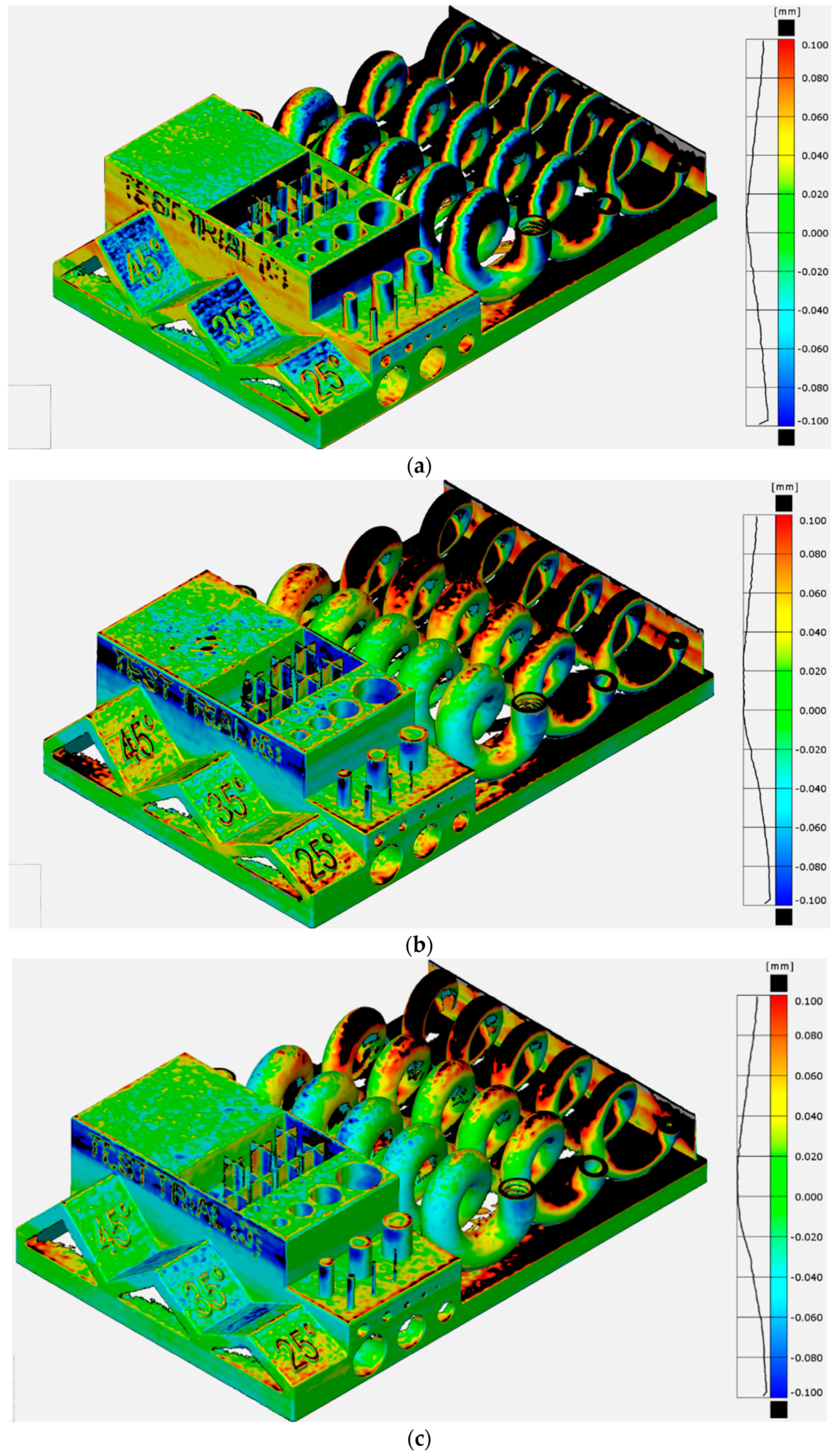
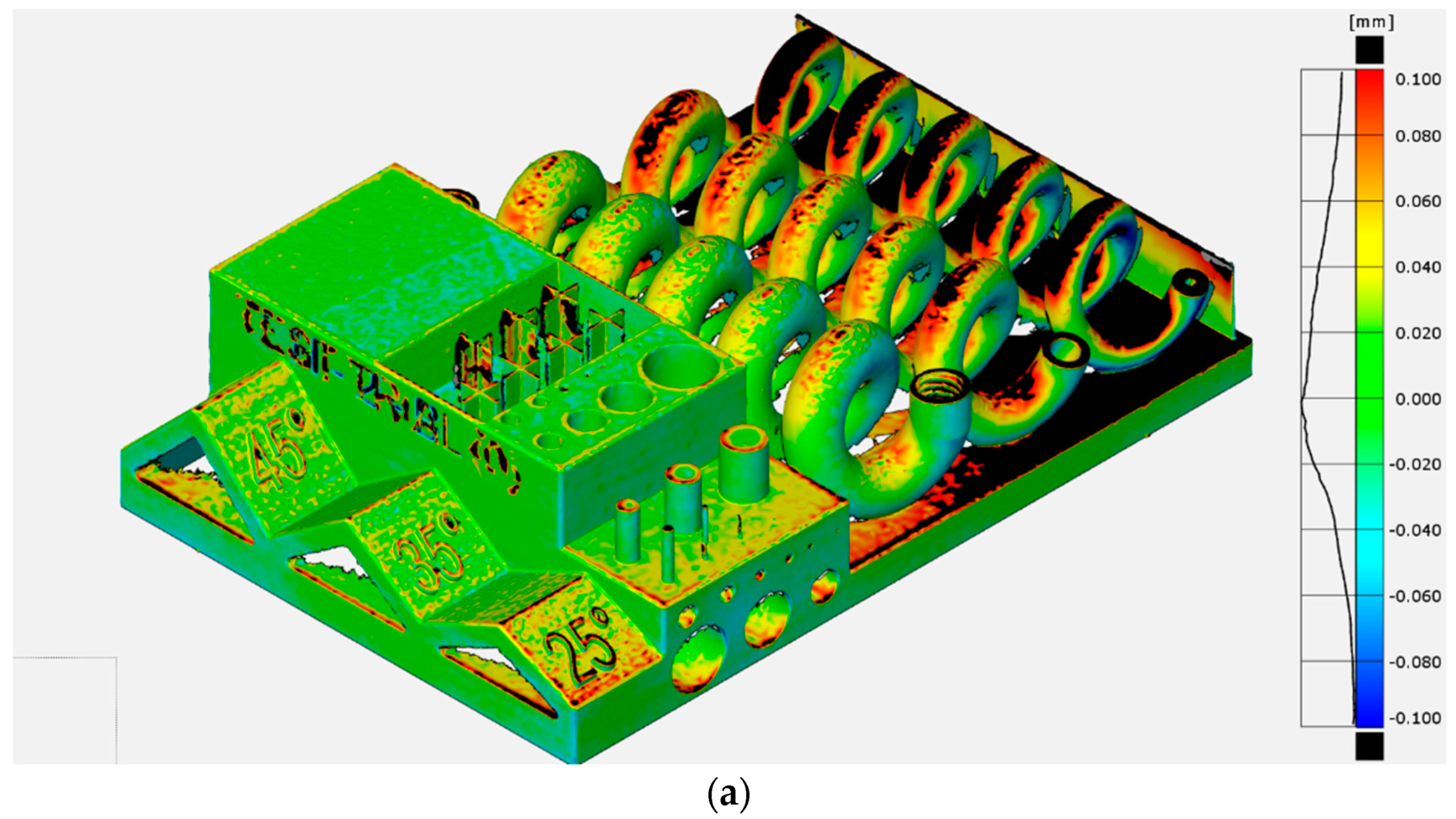
Color plot of the entire first job from G, 3D scanner top alignment. (a) BL, (b) BR, (c) C, (d) TL, (e) TR.
Figure 13.
Color plot of the entire first job from G, 3D scanner top alignment. (a) BL, (b) BR, (c) C, (d) TL, (e) TR.


Figure 14.
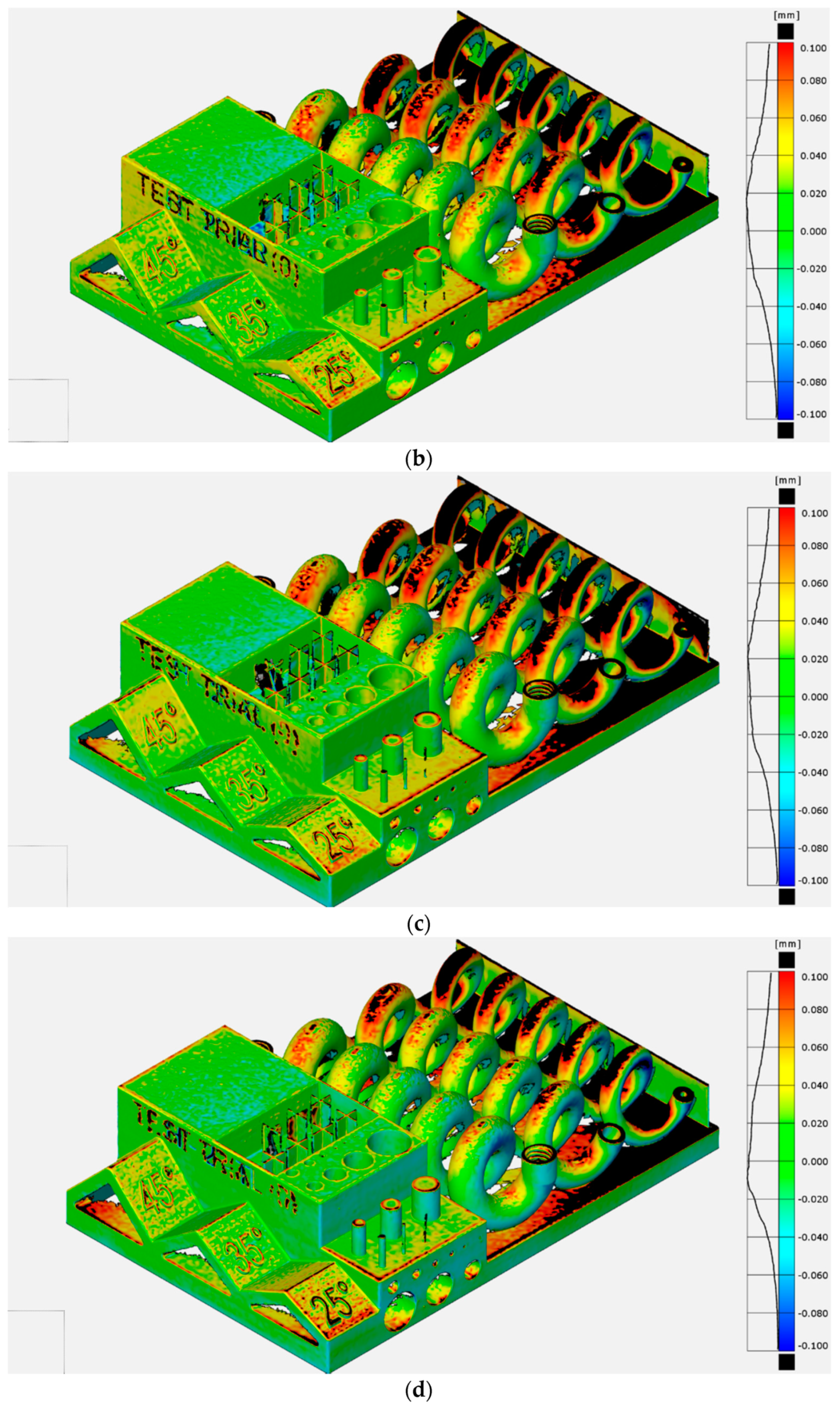
Color plot from the entire second job from company H; 3D scanner top alignment. (a) BL, (b) BR, (c) C, (d) TL, (e) TR.
Figure 14.
Color plot from the entire second job from company H; 3D scanner top alignment. (a) BL, (b) BR, (c) C, (d) TL, (e) TR.


Figure 15.
Comparison of the thin wall color plots from companies C and H. (a) sample BL from company C, 1st job, (b) sample BL from company H, 1st job.
Figure 15.
Comparison of the thin wall color plots from companies C and H. (a) sample BL from company C, 1st job, (b) sample BL from company H, 1st job.

Figure 16.
Picture of the real sample from company C, first job, BL.

Figure 17.
Optical microscope analysis of 2 mm pins from selected participants.

Figure 18.
Deviation graph of the pin diameters compared to nominal CAD dimension produced with GOM Inspect for each pin from each company (in the graph, company F is referred to as company I).
Figure 18.
Deviation graph of the pin diameters compared to nominal CAD dimension produced with GOM Inspect for each pin from each company (in the graph, company F is referred to as company I).

Figure 19.
Optical microscope analysis of 0.10 mm and 0.15 mm thick crosses from selected participants. Each picture presents a short description below.
Figure 19.
Optical microscope analysis of 0.10 mm and 0.15 mm thick crosses from selected participants. Each picture presents a short description below.

Figure 20.
Deviation graph of the cross wall thickness compared to the nominal CAD dimension produced with GOM Inspect for each cross from each company (in the graph, company F is referred to as company I).
Figure 20.
Deviation graph of the cross wall thickness compared to the nominal CAD dimension produced with GOM Inspect for each cross from each company (in the graph, company F is referred to as company I).

Figure 21.
Deviation graph of the hole diameters compared to nominal CAD dimensions produced with GOM Inspect for each hole from each company (in the graph, company F is referred to as company I).
Figure 21.
Deviation graph of the hole diameters compared to nominal CAD dimensions produced with GOM Inspect for each hole from each company (in the graph, company F is referred to as company I).

Figure 22.
Optical microscope pictures of selected holes: diameter of 1.5 mm and 1.2 mm, F, first job, central sample (left); diameter of 1.5 mm and 1.2 mm, H, first job, central sample (right).
Figure 22.
Optical microscope pictures of selected holes: diameter of 1.5 mm and 1.2 mm, F, first job, central sample (left); diameter of 1.5 mm and 1.2 mm, H, first job, central sample (right).

Figure 23.
Deviation graph of pyramid inclination measurements compared to the nominal CAD dimensions produced with GOM Inspect for each pyramid from each company (in the graph, company F is referred as company I).
Figure 23.
Deviation graph of pyramid inclination measurements compared to the nominal CAD dimensions produced with GOM Inspect for each pyramid from each company (in the graph, company F is referred as company I).

Figure 24.
Observed defects on the spiral samples: pyramids from company D, first job, C sample (left); recoater issue from company D, first job, T sample (right).
Figure 24.
Observed defects on the spiral samples: pyramids from company D, first job, C sample (left); recoater issue from company D, first job, T sample (right).

Figure 25.
Ra (μm) represents the comparison for each direction across players. Roughness on the (a) X, (b) Y, (c) Z, (d) T directions.
Figure 25.
Ra (μm) represents the comparison for each direction across players. Roughness on the (a) X, (b) Y, (c) Z, (d) T directions.

Figure 26.
Percentage of residual defects on the polished surfaces of the (a) XY, (b) XZ surfaces.

Figure 27.
Residual defect, company C: XY face (left), XZ face (right).

Figure 28.
Rockwell hardness C (HRC) values across the selected companies: XY face (left); XZ face (right).
Figure 28.
Rockwell hardness C (HRC) values across the selected companies: XY face (left); XZ face (right).

Figure 29.
Tall parts produced by selected companies: company A (left), company G (right).


Table 1.
Examples of benchmarking of additive manufacturing (AM) technologies. For the AM technologies: SLA, stereolithography; SLS, selective laser sintering; LOM, laminated object manufacturing; FDM, fused deposition modeling.
Table 1.
Examples of benchmarking of additive manufacturing (AM) technologies. For the AM technologies: SLA, stereolithography; SLS, selective laser sintering; LOM, laminated object manufacturing; FDM, fused deposition modeling.
| Ref. | Year | AM Tech | Materials | Comments |
|---|---|---|---|---|
| [16] | 2004 | SLA, SLS, LOM, FDM | Different plastics | Comparative evaluation of AM processes, incorporating features from different benchmarking (dimensions: 170 × 170 × 20 mm). |
| [17] | 2005 | SLS, LPBF | Different metal alloys | Thin plate with multiple features (dimensions: 50 × 50 × 9 mm). |
| [18] | 2006 | SLS | Steel-based alloys | Design derived from a real component: half die of a glass bottle (dimensions: 200 × 100 × 40 mm). |
| [19] | 2006 | BJ | Different plastics | Development of a methodology to classify the accuracy of printed parts. |
| [20] | 2007 | LPBF | TiAl6V4 and Co–Cr–Mo | Investigation of medical parts production. |
| [21] | 2010 | SLS | Bronze-based metal | Same features repeated in different orientations in different positions (dimensions of small features: 20 × 20 × 20 mm). |
| [22] | 2010 | BJ | Mixture of polymers | Systematic investigation of the influence of 4 process parameters on the quality and accuracy of green parts. |
| [23] | 2011 | FDM | ABS | Quantitative evaluation of open-source 3D printer. |
| [24] | 2011 | MJ, SLA, SLS, FDM | Different plastics | Simple and quick method to compare speed and accuracy of AM technologies. |
| [25] | 2012 | SLS | Nylon | Focus on accuracy and repeatability (dimensions: 270 × 50 mm). |
| [14] | 2014 | Several AM techs | Several materials | Moylan et al.’s standardization proposal (dimensions: 100 × 100 × 10 mm). |
| [26] | 2015 | SLS, SLA, MJ | Different plastics | Definition of a DoE to optimize the manufacturing of a mass-production consumer device geometry. |
Table 2.
Investigation criteria of benchmarking.
| General Aspect | Specification | Comments |
|---|---|---|
| Accuracy | Dimension of feature | Various features visible in Figure 3, with minimum dimensions that go beyond the currently known machine’s limitation (see Table 3). |
| Surface roughness | Important factor considering industrial production and current need for post-processing parts to achieve specified roughness. | |
| Repeatability | Same job, different positions | Evaluated by repeating production of the same part in 4 corners of the machine’s building volume and centre of the building platform; extremely important considering industrial need for a robust and reliable process. |
| Different jobs | Same as above; each job repeated 3 times. | |
| Complex feature | Spiral shape: mold’s cooling channel | Overview of machine capabilities in handling complex features that can be related to real applications such as conformal cooling channels in molds. |
| Homogeneity | Residual defects | Indicator of process quality. |
| Density | ||
| Residual stress | Part distortions | Related to robustness of the process and final quality of the product in terms of how close they are to the nominal design. |
| Mechanical properties | Rockwell hardness C | General indicator of quality of the material. |
| Built speed | To compare the speed of various machines. | |
| Tall parts production | Tall samples | Understanding of machine capabilities in building relatively tall parts. |
Table 3.
Minimum dimension of features presented in benchmarking artifact.
| Feature | Minimum Dimension | Min Dimension in Artifact |
|---|---|---|
| Wall thickness | 0.15 mm | 0.10 mm |
| Overhang structure | 45° | 25° |
| Circular holes (diameter) | 0.50 mm | 0.20 mm |
| Circular pins (diameter) | 0.50 mm | 0.10 mm |
Table 4.
Chemical composition of maraging steel (st-%) [31].
Table 4.
Chemical composition of maraging steel (st-%) [31].
| Fe | Ni | Co | Mo | Ti | Al | Cr, Cu | C | Mn, Si | P, S |
|---|---|---|---|---|---|---|---|---|---|
| Bal | 17–19% | 8.5–9.5% | 4.5–5.2% | 0.6–0.8% | 0.05–0.15% | Each ≤0.5% | ≤0.03% | Each ≤0.1% | Each ≤0.01% |
Table 5.
Surface roughness measurement specifications.
| Ra Range | 2–10 μm |
|---|---|
| Evaluation length | 12.5 mm |
| Sample length | 2.5 mm |
| λc | 2.5 mm |
| λf | 0.08 mm |
| Number of cut-offs | 5 |
| Surface | Aperiodic |
| Filter | Gaussian |
Table 6.
Machines evaluated in this benchmarking. Machine H is the only one whose information will be shared: Yb fiber laser, max power 200 W, building platform 250 × 250 mm, nitrogen atmosphere, hard ceramic recoater.
Table 6.
Machines evaluated in this benchmarking. Machine H is the only one whose information will be shared: Yb fiber laser, max power 200 W, building platform 250 × 250 mm, nitrogen atmosphere, hard ceramic recoater.
| Company | Type of Company | No. Lasers Used | Cutting Technology | Layer Thickness [μm] |
|---|---|---|---|---|
| A | Machine manufacturer | 1 | Wire EDM | 40 |
| B | Machine manufacturer | 1 | Wire EDM | 30 |
| C | Machine manufacturer | 2 | 2 jobs: wire EDM 1 job: band saw | 30 |
| D | Machine manufacturer | 1 | Wire EDM | 40 |
| E | End user (machine owner) | 2 | – | 40 |
| F | Machine manufacturer | 4 | Wire EDM | 40 |
| G | End user (machine owner) | 1 | Band saw | 40 |
| H | End user (machine owner) | 1 | Band saw | 40 |
Table 7.
Pin construction summary for each company. ✓ acceptable; ≈ uncertain; ✗ not built.
| Supplier | Pin | 1 | 2 | 3 | 4 | 5 | 6 | 7 | 8 |
|---|---|---|---|---|---|---|---|---|---|
| A | TL | ✗✗✗ | ✗✗✗ | ✗✓✓ | ✗✗≈ | ✓✓✓ | ✓✓✓ | ✓✓✓ | ✓✓✓ |
| TR | ✗✗✗ | ✗✗✗ | ✗✓✗ | ✗✗≈ | ✓✓✓ | ✓✓✓ | ✓✓✓ | ✓✓✓ | |
| C | ✗✗✗ | ✗≈✗ | ✓✓✓ | ✗≈✗ | ✓✓✓ | ✓✓✓ | ✓✓✓ | ✓✓✓ | |
| BL | ✗✗✗ | ✗✗✗ | ✗✓≈ | ✗≈≈ | ✓✓✓ | ✓✓✓ | ✓✓✓ | ✓✓✓ | |
| BR | ✗✗✗ | ✗✗✗ | ✓✗✓ | ✗✗✗ | ✓✓✓ | ✓✓✓ | ✓✓✓ | ✓✓✓ | |
| B | TL | ✗≈✗ | ≈✗✗ | ✓✓✓ | ✓✓✓ | ✓✓✓ | ✓✓✓ | ✓✓✓ | ✓✓✓ |
| TR | ✗✗≈ | ≈≈≈ | ✓✓✓ | ✓✓✓ | ✓✓✓ | ✓✓✓ | ✓✓✓ | ✓✓✓ | |
| C | ✗✗≈ | ≈≈≈ | ✓✓✓ | ✓✓✓ | ✓✓✓ | ✓✓✓ | ✓✓✓ | ✓✓✓ | |
| BL | ✗≈✗ | ≈≈✗ | ✓✓✓ | ✓✓✓ | ✓✓✓ | ✓✓✓ | ✓✓✓ | ✓✓✓ | |
| BR | ✗≈≈ | ≈≈≈ | ✓✓✓ | ✓✓✓ | ✓✓✓ | ✓✓✓ | ✓✓✓ | ✓✓✓ | |
| C | TL | ≈≈≈ | ≈≈≈ | ✓✓✓ | ✓✓✓ | ✓✓✓ | ✓✓✓ | ✓✓✓ | ✓✓✓ |
| TR | ≈≈≈ | ≈≈≈ | ✓✓✓ | ✓✓✓ | ✓✓✓ | ✓✓✓ | ✓✓✓ | ✓✓✓ | |
| C | ≈≈≈ | ≈≈≈ | ✓✓✓ | ✓✓✓ | ✓✓✓ | ✓✓✓ | ✓✓✓ | ✓✓✓ | |
| BL | ≈≈≈ | ≈≈≈ | ✓✓✓ | ✓✓✓ | ✓✓✓ | ✓✓✓ | ✓✓✓ | ✓✓✓ | |
| BR | ≈≈≈ | ≈≈≈ | ✓✓✓ | ✓✓✓ | ✓✓✓ | ✓✓✓ | ✓✓✓ | ✓✓✓ | |
| D | R | ✗✗✗ | ≈✗✗ | ✓✓✓ | ✓✓✓ | ✓✓✓ | ✓✓✓ | ✓✓✓ | ✓✓✓ |
| T | ✗✗✗ | ✗≈✗ | ✓✓✓ | ✓✓✓ | ✓✓✓ | ✓✓✓ | ✓✓✓ | ✓✓✓ | |
| C | ✗✗✗ | ✗✗✗ | ✓✓✗ | ✓✓✓ | ✓✓✓ | ✓✓✓ | ✓✓✓ | ✓✓✓ | |
| L | ✗✗✗ | ✗✗≈ | ✓✓✓ | ✓✓✓ | ✓✓✓ | ✓✓✓ | ✓✓✓ | ✓✓✓ | |
| B | ✗✗✗ | ✗✗✗ | ✓✓✗ | ✓✓✓ | ✓✓✓ | ✓✓✓ | ✓✓✓ | ✓✓✓ | |
| F | TL | ✗✗✗ | ✗✗✗ | ✗✗✗ | ✓✓✓ | ✓✓✓ | ✓✓✓ | ✓✓✓ | ✓✓✓ |
| TR | ✗✗✗ | ✗✗✗ | ✓✗✓ | ✓✓✓ | ✓✓✓ | ✓✓✓ | ✓✓✓ | ✓✓✓ | |
| C | ✗✗✗ | ✗✗✗ | ✓≈✗ | ✓✓✓ | ✓✓✓ | ✓✓✓ | ✓✓✓ | ✓✓✓ | |
| BL | ✗✗✗ | ✗✗✗ | ✗✗✗ | ✓✓✓ | ✓✓✓ | ✓✓✓ | ✓✓✓ | ✓✓✓ | |
| BR | ✗✗✗ | ✗✗✗ | ✓✓✓ | ✓✓✓ | ✓✓✓ | ✓✓✓ | ✓✓✓ | ✓✓✓ | |
| G | TL | ✗✗✗ | ✗≈✗ | ✓✓✓ | ✓✓✓ | ✓✓✓ | ✓✓✓ | ✓✓✓ | ✓✓✓ |
| TR | ✗✗✗ | ✗✗✗ | ✓✓✓ | ✓✓✓ | ✓✓✓ | ✓✓✓ | ✓✓✓ | ✓✓✓ | |
| C | ✗✗✗ | ✗✗✗ | ✓✓✓ | ✓✓✓ | ✓✓✓ | ✓✓✓ | ✓✓✓ | ✓✓✓ | |
| BL | ✗✗✗ | ✗✗✗ | ✓✓✓ | ✓✓✓ | ✓✓✓ | ✓✓✓ | ✓✓✓ | ✓✓✓ | |
| BR | ✗✗✗ | ✗≈≈ | ✓✓✓ | ✓✓✓ | ✓✓✓ | ✓✓✓ | ✓✓✓ | ✓✓✓ | |
| H | TL | ✗✗✗ | ✗✗≈ | ✓✓✓ | ✓✓✓ | ✓✓✓ | ✓✓✓ | ✓✓✓ | ✓✓✓ |
| TR | ✗✗✗ | ≈≈✗ | ✓✗✓ | ✓✓✓ | ✓✓✓ | ✓✓✓ | ✓✓✓ | ✓✓✓ | |
| C | ✗✗✗ | ✗✗✗ | ✓✓✓ | ✓✓✓ | ✓✓✓ | ✓✓✓ | ✓✓✓ | ✓✓✓ | |
| BL | ✗✗✗ | ≈≈≈ | ✗✗✓ | ✓✓≈ | ✓✓✓ | ✓✓✓ | ✓✓✓ | ✓✓✓ | |
| BR | ✗✗✗ | ✗≈✗ | ✓✓✗ | ✓✓✓ | ✓✓✓ | ✓✓✓ | ✓✓✓ | ✓✓✓ |
Table 8.
Cross construction summary for each company. ✓ acceptable; ≈ existing feature, oversize; ✓ existing feature, not acceptable; ✗ not built.
Table 8.
Cross construction summary for each company. ✓ acceptable; ≈ existing feature, oversize; ✓ existing feature, not acceptable; ✗ not built.
| Supplier | Cross | 1 | 2 | 3 | 4 | 5 | 6 | 7 | 8 |
|---|---|---|---|---|---|---|---|---|---|
| A | TL | ✗✗✗ | ✗✗✗ | ✓✓✓ | ✓✓✓ | ✓✓✓ | ✓✓✓ | ✓✓✓ | ✓✓✓ |
| TR | ✗✗✗ | ✗✗✗ | ✓✓✓ | ✓✓✓ | ✓✓✓ | ✓✓✓ | ✓✓✓ | ✓✓✓ | |
| C | ✗✗✗ | ✗✗✗ | ✓✓✓ | ✓✓✓ | ✓✓✓ | ✓✓✓ | ✓✓✓ | ✓✓✓ | |
| BL | ✗✗✗ | ✗✗✗ | ✓✓✓ | ✓✓✓ | ✓✓✓ | ✓✓✓ | ✓✓✓ | ✓✓✓ | |
| BR | ✗✗✗ | ✗✗✗ | ✓✓✓ | ✓✓✓ | ✓✓✓ | ✓✓✓ | ✓✓✓ | ✓✓✓ | |
| B | TL | ✓✓✓ | ✓✓✓ | ✓✓✓ | ✓✓✓ | ✓✓✓ | ✓✓✓ | ✓✓✓ | ✓✓✓ |
| TR | ✓✓✓ | ✓✓✓ | ✓✓✓ | ✓✓✓ | ✓✓✓ | ✓✓✓ | ✓✓✓ | ✓✓✓ | |
| C | ✓✓✓ | ✓✓✓ | ✓✓✓ | ✓✓✓ | ✓✓✓ | ✓✓✓ | ✓✓✓ | ✓✓✓ | |
| BL | ✓✓✗ | ✓✓✓ | ✓✓✓ | ✓✓✓ | ✓✓✓ | ✓✓✓ | ✓✓✓ | ✓✓✓ | |
| BR | ✓✓✓ | ✓✓✓ | ✓✓✓ | ✓✓✓ | ✓✓✓ | ✓✓✓ | ✓✓✓ | ✓✓✓ | |
| C | TL | ≈≈≈ | ≈≈≈ | ✓✓✓ | ✓✓✓ | ✓✓✓ | ✓✓✓ | ✓✓✓ | ✓✓✓ |
| TR | ≈≈≈ | ≈≈≈ | ✓✓✓ | ✓✓✓ | ✓✓✓ | ✓✓✓ | ✓✓✓ | ✓✓✓ | |
| C | ≈≈≈ | ≈≈≈ | ✓✓✓ | ✓✓✓ | ✓✓✓ | ✓✓✓ | ✓✓✓ | ✓✓✓ | |
| BL | ≈≈≈ | ≈≈≈ | ✓✓✓ | ✓✓✓ | ✓✓✓ | ✓✓✓ | ✓✓✓ | ✓✓✓ | |
| BR | ≈≈≈ | ≈≈≈ | ✓✓✓ | ✓✓✓ | ✓✓✓ | ✓✓✓ | ✓✓✓ | ✓✓✓ | |
| D | R | ✓✓✓ | ✓✓✓ | ✓✓✓ | ✓✓✓ | ✓✓✓ | ✓✓✓ | ✓✓✓ | ✓✓✓ |
| T | ✓✓✓ | ✓✓✓ | ✓✓✓ | ✓✓✓ | ✓✓✓ | ✓✓✓ | ✓✓✓ | ✓✓✓ | |
| C | ✓✓✓ | ✓✓✓ | ✓✓✓ | ✓✓✓ | ✓✓✓ | ✓✓✓ | ✓✓✓ | ✓✓✓ | |
| L | ✓✓✓ | ✓✓✓ | ✓✓✓ | ✓✓✓ | ✓✓✓ | ✓✓✓ | ✓✓✓ | ✓✓✓ | |
| B | ✓✓✓ | ✓✓✓ | ✓✓✓ | ✓✓✓ | ✓✓✓ | ✓✓✓ | ✓✓✓ | ✓✓✓ | |
| F | TL | ✓✓✓ | ✓✓✓ | ✓✓✓ | ✓✓✓ | ✓✓✓ | ✓✓✓ | ✓✓✓ | ✓✓✓ |
| TR | ✓✓✓ | ✓✓✓ | ✓✓✓ | ✓✓✓ | ✓✓✓ | ✓✓✓ | ✓✓✓ | ✓✓✓ | |
| C | ✓✓✓ | ✓✓✓ | ✓✓✓ | ✓✓✓ | ✓✓✓ | ✓✓✓ | ✓✓✓ | ✓✓✓ | |
| BL | ✓✓✓ | ✓✓✓ | ✓✓✓ | ✓✓✓ | ✓✓✓ | ✓✓✓ | ✓✓✓ | ✓✓✓ | |
| BR | ✓✓✓ | ✓✓✓ | ✓✓✓ | ✓✓✓ | ✓✓✓ | ✓✓✓ | ✓✓✓ | ✓✓✓ | |
| G | TL | ✗✗✗ | ✓✓✓ | ✓✓✓ | ✓✓✓ | ✓✓✓ | ✓✓✓ | ✓✓✓ | ✓✓✓ |
| TR | ✗✗✗ | ✓✓✓ | ✓✓✓ | ✓✓✓ | ✓✓✓ | ✓✓✓ | ✓✓✓ | ✓✓✓ | |
| C | ✗✗✗ | ✓✓✓ | ✓✓✓ | ✓✓✓ | ✓✓✓ | ✓✓✓ | ✓✓✓ | ✓✓✓ | |
| BL | ✗✗✗ | ✓✓✓ | ✓✓✓ | ✓✓✓ | ✓✓✓ | ✓✓✓ | ✓✓✓ | ✓✓✓ | |
| BR | ✗✗✗ | ✓✓✓ | ✓✓✓ | ✓✓✓ | ✓✓✓ | ✓✓✓ | ✓✓✓ | ✓✓✓ | |
| H | TL | ✗✗✗ | ✓✓✓ | ✓✓✓ | ✓✓✓ | ✓✓✓ | ✓✓✓ | ✓✓✓ | ✓✓✓ |
| TR | ✗✗✗ | ✓✓✓ | ✓✓✓ | ✓✓✓ | ✓✓✓ | ✓✓✓ | ✓✓✓ | ✓✓✓ | |
| C | ✗✗✗ | ✓✓✓ | ✓✓✓ | ✓✓✓ | ✓✓✓ | ✓✓✓ | ✓✓✓ | ✓✓✓ | |
| BL | ✗✗✗ | ✓✓✓ | ✓✓✓ | ✓✓✓ | ✓✓✓ | ✓✓✓ | ✓✓✓ | ✓✓✓ | |
| BR | ✗✗✗ | ✓✓✓ | ✓✓✓ | ✓✓✓ | ✓✓✓ | ✓✓✓ | ✓✓✓ | ✓✓✓ |
Table 9.
Collection of results on surface roughness, Ra μm.
| Company | Direction | Job | Avg | Std.-Dev | Company | Direction | Job | Avg | Std.-Dev |
|---|---|---|---|---|---|---|---|---|---|
| A | X | 1 | 9.5 | 0.7 | F | X | 1 | 6.5 | 0.4 |
| 2 | 8.9 | 0.7 | 2 | 6.1 | 0.6 | ||||
| 3 | 9.6 | 0.9 | 3 | 5.6 | 0.2 | ||||
| Y | 1 | 9.9 | 0.6 | Y | 1 | 6.9 | 1.0 | ||
| 2 | 8.8 | 0.6 | 2 | 6.7 | 0.4 | ||||
| 3 | 8.3 | 1.1 | 3 | 6.3 | 0.9 | ||||
| Z | 1 | 6.1 | 0.5 | Z | 1 | 10.1 | 1.3 | ||
| 2 | 6.3 | 0.2 | 2 | 9 | 1 | ||||
| 3 | 6.5 | 0.5 | 3 | 11 | 1 | ||||
| T | 1 | 6.7 | 1.0 | T | 1 | 10.6 | 1.4 | ||
| 2 | 6.3 | 0.4 | 2 | 9.6 | 0.8 | ||||
| 3 | 5.9 | 0.7 | 3 | 10 | 1 | ||||
| B | X | 1 | 12.6 | 0.4 | G | X | 1 | 9.9 | 0.2 |
| 2 | 10.6 | 1.9 | 2 | 8.9 | 0.7 | ||||
| 3 | 10.6 | 1.9 | 3 | 8.6 | 1.2 | ||||
| Y | 1 | 10.3 | 0.4 | Y | 1 | 8.3 | 0.1 | ||
| 2 | 10.1 | 0.2 | 2 | 9.4 | 0.9 | ||||
| 3 | 10.4 | 1.1 | 3 | 8.7 | 0.4 | ||||
| Z | 1 | 9.2 | 0.8 | Z | 1 | 8.0 | 0.9 | ||
| 2 | 11.4 | 0.3 | 2 | 6.4 | 0.3 | ||||
| 3 | 8.6 | 0.6 | 3 | 7.8 | 0.2 | ||||
| T | 1 | 9.7 | 0.4 | 1 | 5.5 | 1.7 | |||
| 2 | 10.8 | 1 | T | 2 | 5.0 | 0.3 | |||
| 3 | 8.9 | 0.3 | 3 | 5.3 | 0.5 | ||||
| C | X | 1 | 10.8 | 0.2 | H | X | 1 | 7.1 | 0.9 |
| 2 | 11.5 | 0.3 | 2 | 5.2 | 0.5 | ||||
| 3 | 9.9 | 0.6 | 3 | 6.1 | 0.4 | ||||
| Y | 1 | 10.1 | 1.1 | Y | 1 | 6.1 | 0.6 | ||
| 2 | 9.8 | 0.7 | 2 | 6.2 | 0.6 | ||||
| 3 | 10.1 | 0.7 | 3 | 6.1 | 0.3 | ||||
| Z | 1 | 7.7 | 0.3 | Z | 1 | 5.4 | 0.7 | ||
| 2 | 7.8 | 0.5 | 2 | 5.2 | 0.5 | ||||
| 3 | 9.3 | 0.3 | 3 | 6.2 | 0.3 | ||||
| T | 1 | 7.0 | 0.6 | T | 1 | 5.1 | 0.9 | ||
| 2 | 7.7 | 0.8 | 2 | 5.2 | 0.4 | ||||
| 3 | 9.7 | 0.5 | 3 | 5.7 | 0.33 | ||||
| D | X | 1 | 6.9 | 0.5 | |||||
| 2 | 19.9 | 6.4 | |||||||
| 3 | 11.7 | 0.5 | |||||||
| Y | 1 | 18.9 | 2.1 | ||||||
| 2 | 19.2 | 3 | |||||||
| 3 | 10 | 1.2 | |||||||
| Z | 1 | 6.2 | 0.4 | ||||||
| 2 | 7.5 | 0.4 | |||||||
| 3 | 8 | 1.2 | |||||||
| T | 1 | 5.9 | 0.1 | ||||||
| 2 | 7.6 | 0.6 | |||||||
| 3 | 8.6 | 1.9 |
Table 10.
Density and relative density for each supplier.
| Company | Density (g/cm3) | Relative Density (%) |
|---|---|---|
| A | 8.05 | 99.4 |
| B | 8.04 | 99.3 |
| C | 8.07 | 99.6 |
| D | 7.98 | 98.5 |
| F | 8.06 | 99.5 |
| G | 8.05 | 99.4 |
| H | 8.06 | 99.5 |
Table 11.
Percentage of residual defects visible on polished surfaces.
| Company | Face XY | Face Z |
|---|---|---|
| A | 0.02% | 0.01% |
| C | 0.09% | 2.6% |
| F | 0.06% | 0.4% |
| G | 0.07% | 0.7% |
| H | 0.04% | 0.04% |
Table 12.
Build time (in hours) for each company to produce one job.
| A (1 Laser) | B (1 Laser) | C (2 Laser) | D (1 Laser) | F (4 Lasers) | G (1 Laser) | H (1 Laser) |
|---|---|---|---|---|---|---|
| 40.5–49.5 | 52.6 | 50–65 | 66–80 | 24–25 | 60–62 | 52–53 |
Table 13.
Results overview and discussion.
| General Aspect | Specifications | Results and Discussion |
|---|---|---|
| Accuracy | Dimension of feature | Most features measured overcame limitations stated by machine manufacturers in Table 3. |
| Surface roughness | Surface roughness revealed for most companies’ discontinuities in Ra value among jobs depended on the directions; in general, between all samples, Ra was never lower than 5.0 ± 0.3 μm (G-T-2). | |
| Repeatability | Same job, different positions | Color plot analysis shows there was total repeatability among positions and/or jobs for none of the companies; however, differences could have been appreciated between companies. |
| Different jobs | ||
| Complex feature | Spiral shape: mold’s cooling channel | All companies managed to produce good quality spiral features, well handling complex geometries. |
| Homogeneity | Residual defects | Most companies had density higher than 99%, as expected, during Archimedes analysis; in polished surface analysis some differences of residual defects could be seen, even if most participants did not overstep 0.1% of defects on both surfaces. |
| Density | ||
| Residual stress | Part distortions | Thin wall showed, especially in some cases, great distortions coming from process that would need to be considered for production of end products with tight tolerance; during analysis of repeatability it was possible to appreciate part distortion of overall spiral sample. |
| Mechanical properties | Rockwell hardness C | Measurements did not reveal discontinuity of products from any company, recording expected HRC value. |
| Built speed | Time required for production was important input for readiness of use of LPBF for industrial production as well as an indication of the recent direction of technology development. | |
| Tall parts production | Tall samples | Tall parts production (with a small base) presented issues for only one company, confirming that it does not represent a current problem. |
© 2019 by the authors. Licensee MDPI, Basel, Switzerland. This article is an open access article distributed under the terms and conditions of the Creative Commons Attribution (CC BY) license (http://creativecommons.org/licenses/by/4.0/).
Share and Cite
MDPI and ACS Style
Moshiri, M.; Candeo, S.; Carmignato, S.; Mohanty, S.; Tosello, G. Benchmarking of Laser Powder Bed Fusion Machines. J. Manuf. Mater. Process. 2019, 3, 85. https://0-doi-org.brum.beds.ac.uk/10.3390/jmmp3040085
AMA Style
Moshiri M, Candeo S, Carmignato S, Mohanty S, Tosello G. Benchmarking of Laser Powder Bed Fusion Machines. Journal of Manufacturing and Materials Processing. 2019; 3(4):85. https://0-doi-org.brum.beds.ac.uk/10.3390/jmmp3040085
Chicago/Turabian StyleMoshiri, Mandaná, Stefano Candeo, Simone Carmignato, Sankhya Mohanty, and Guido Tosello. 2019. "Benchmarking of Laser Powder Bed Fusion Machines" Journal of Manufacturing and Materials Processing 3, no. 4: 85. https://0-doi-org.brum.beds.ac.uk/10.3390/jmmp3040085