1. Introduction
The importance of the acoustic emission (AE) sensor has been shown for the monitoring, controlling, and predicting of the machining process [
1]. Given that, the use of AE sensors has been under expansion in different fields of science and industry. The AE signal, generated during the grinding processes, has been verified to be related to the process state and the surface condition of the grinding tool and workpiece [
2]. By using this approach, researchers are able to improve different aspects of machining, such as detection of the wheel wear and loading, chatter analysis, detection of the collision, detection of the machining burn and cracks, gap elimination, process control, and dressing/truing verification [
3].
Artificial neural networks (ANNs) are computing systems that are stimulated by biological neural networks (NNs). Such systems learn how to perform tasks without being notably programmed. NNs represent the most effective machine learning technology in general, and more specifically, in the research and development. The ANNs are the leading machine-learning tools in several domains, such as image analysis and fault diagnosis. The number of research publications recorded exponential growth during the last three years [
4,
5,
6,
7].
The grinding process is generally the final steps of machining of precise workpieces and accounts for about 20%–25% of the total investments in machining operations in industrialized countries [
8]. Therefore, the surface roughness of ground parts is an essential factor for the assessment of the grinding process, and an important criterion for choosing the machine tool, the dressing and grinding tools and parameter [
9]. As a result of the intensified potential for high productivity, low cost, and high-grade quality of grinding products, online condition monitoring and feedback control of grinding processes are highly demanded by industry [
10]. The quality of the ground surface contains various characteristics, such as burned area, surface roughness, residual stresses, phase transformation and also cracks throughout the workpiece. However, many other marks can be found on the surface, such as cracks produced by the thermal impact, back transferred material, and craters produced by the grain fracture [
11].
In modeling of the grinding process, a few researches, dealing with the fundamental understanding of the material removal mechanisms (single grain-workpiece interaction), are available [
12,
13,
14]. Moreover, the micro-scale numerical modelling methods are developed to describe the plastic behavior of the workpiece material at the high temperature and strain-rates linked with the grinding process. Zahedi and Azarhoushang [
15] simulated the interaction of cubic Born Nitride (cBN) cutting grains with a bearing steel workpiece using the finite element method (FEM), and showed that the calculated forces are qualitatively in accordance with the experimental data.
Lin et al. [
7] estimated the properties of grinding wheel condition for grinding of hard and brittle materials. They showed that most of the grinding information could be analyzed based on AE spectra analysis at the frequency bands of 600–900 kHz. The topography of the grinding wheel could also be described using discrete wavelet transform and Root Mean Square (RMS) statistics. Adibi et al. [
5] studied the efficiency of AE signals to detect the wheel loading in the grinding of nickel-based superalloy. The results showed that RMS is an appropriate parameter to predict the grinding performance in the case of wheel loading. The surface condition of the grinding wheel was also analyzed using AE signals by Liu and Li [
4]. Their proposed measurement method showed that the grinding wheel loading phenomena could be online evaluated using a quantitative index from the AE signals. Marek Vrab et al. [
16] used the ANNs to predict the surface integrity in the machining process. They developed and tested a neural network that was able to predict the drill flank wear in order to prevent anomalies occurring on the machined surface as and a neural network that can predict surface roughness. They finally showed that it is possible to model and monitor a complex non-linear relationship between process performance parameters and process variables in machining. Their modeling also had a good generalization ability, and appears to be a useful tool in the cutting tool wear condition monitoring when drilling. Additionally, the model could be utilized in surface roughness prediction in monitoring system with the average RMS error percentage of 2.64%. B. Anuja Beatrice et al. [
6] studied the ability of modeling the surface roughness (Ra) in terms of cutting parameters during hard turning of AISI H13 tool steel with minimal cutting fluid application. They showed that the developed ANN model can be a useful tool to fix the cutting parameters in order to achieve a desired surface finish. Heydarzadeh et al. [
17] estimated the cutting forces using ANNs. They used the designed method and proved that it was successfully applied to the precise estimation of micro-milling forces, in order to estimate tool deflections. V Karri et al. [
18] developed a neural network architecture to predict the forces and power in the single-edged oblique cutting operation. In testing the model, the three force components in oblique cutting were predicted to an accuracy of 6% error.
According to the aforementioned studies, the error of the surface roughens prediction via analytical models in the grinding process is very high. The grinding grits on the surface of the grinding tool are stochastically distributed. It is also impossible to find two same abrasive grits with the same shape and cutting edges. Hence, it is difficult to precisely predict the surface roughness with analytical methods, as well as with kinematical methods in the grinding process. There are also several parameters that are influential in the modeling of the grinding forces and surface roughness, such as vibration, the precision of the machine tool, the tool specification, dressing parameters. It is also impossible to consider all affecting parameters in the modeling process. Moreover, there are very few researches in the field of surface roughness prediction using the ANNs.
This work carried out to investigate the application of AE signals for predicting surface roughness and grinding forces with high accuracy with the help of initial grinding parameters as the input data for ANNs. The input parameters were divided into two classifications: The first classification was included only the grinding process parameters
Table 1, and the second classification was for the AE signals. Later, for training the ANNs, these two classifications were added to the ANNs as inputs. The accuracy of these two categories on the prediction of surface roughness and grinding forces was compared. Several experiments with different grinding parameters, i.e., cutting speed, feed rate, and depth of cut were carried out. Using the experimental data, obtained from the grinding process, two various neural networks were trained to model and predict the grinding forces and surface roughens. In the end, the models were validated and tested with experimental data, which was not utilized for the model training. Moreover, the effect of the training rate on the prediction of surface roughness is also investigated.
2. Experimental Procedure
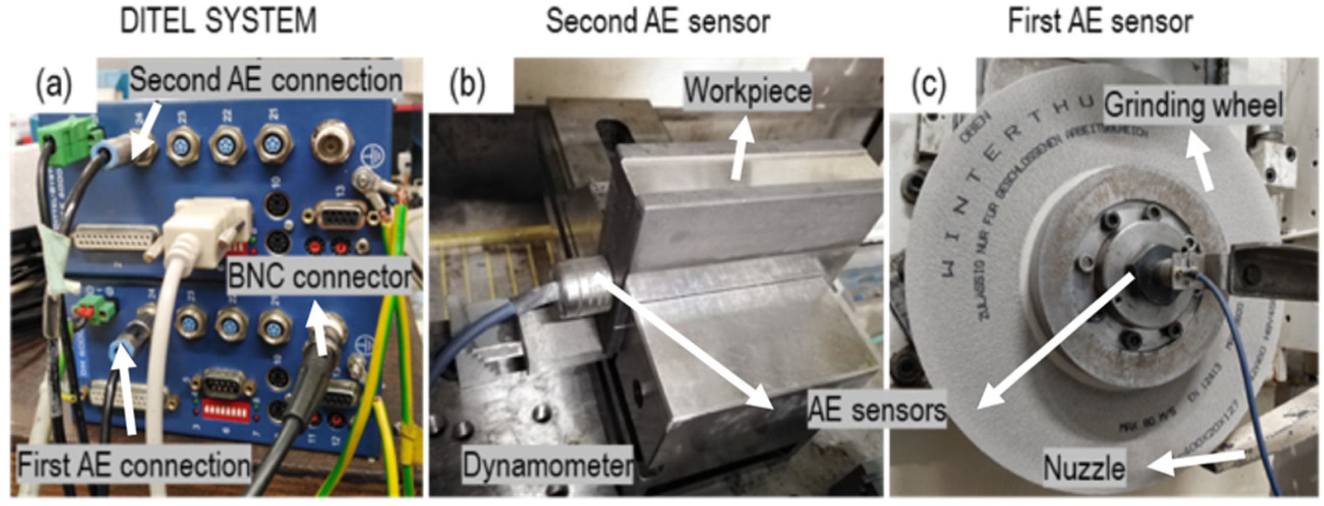
To accomplish the experiments and collecting the Acoustic Emission (AE) signals, 2 desired AE sensors were integrated into a high-performance surface grinding machine Micro-Cut AC8 CNC (Elb-Schliff Werkzeugmaschinen GmbH, Aschaffenburg, Germany).
Figure 1 shows the experimental setup. Two AE sensors from DITTEL (Dittel Messtechnik GmbH, Landsberg am Lech, Germany) was used and the amplifier was likewise from DITTEL company. An AE sensor was attached to the workpiece (
Figure 1b). The center of the AE sensor was placed 4 mm far from the top and 10 mm from the side of the workpiece. Row AE-signals were recorded from this sensor and subjected to filtering and denoising. To have better view and comparable results between AE sensors during grinding, a second AE sensor for monitoring the grinding process was installed close to the center of the grinding wheel (
Figure 1c). This sensor was directly connected to the DITTEL software and the RMS was extracted. The grinding tests were conducted at different cutting speeds (
vc), feed rates (
vw), and depth of cuts (
ae).
Table 1 lists the grinding parameters.
A 42A60 H8V450W grinding wheel was used for the trials. Prior to each grinding test, the wheel was dressed using a diamond roller dresser from Dr Keiser, with the dressing overlap ratio, Ud, of 2, dressing speed ratio, qd, of +0.8, and the dressing depth of cut, aed, of 20 µm. For collecting the AE signals, an oscilloscope Picoscope 4424 from the Pico Technology company St Neots, UK was used. After collecting the AE signal from the Picoscope with the 1 MHz sampling rate, for the further processing of the signal with MATLAB, the signals were saved in MAT (mat extension are files that are in the binary data container format that the MATLAB program uses). To measure the surface roughness Hommel–Werke model T-1000 from JENOPTIK company in Villingen-Schwenningen, Germany was utilized. The chosen material for the experiments was 100Cr6, with dimensions of 80 mm length, 60 mm height, and 40 mm width. Water-soluble coolant (Emulsion. 5%) was applied as the grinding coolant lubricant fluid. A Kistler dynamometer type 5278b was used to measure the grinding forces. The grinding forces were processed with Kistler 5015 charge amplifiers in Winterthur, Switzerland and recorded by a PC acquisition board and LabView software from National Instrument in Austin, TX, USA.
3. Signal Processing
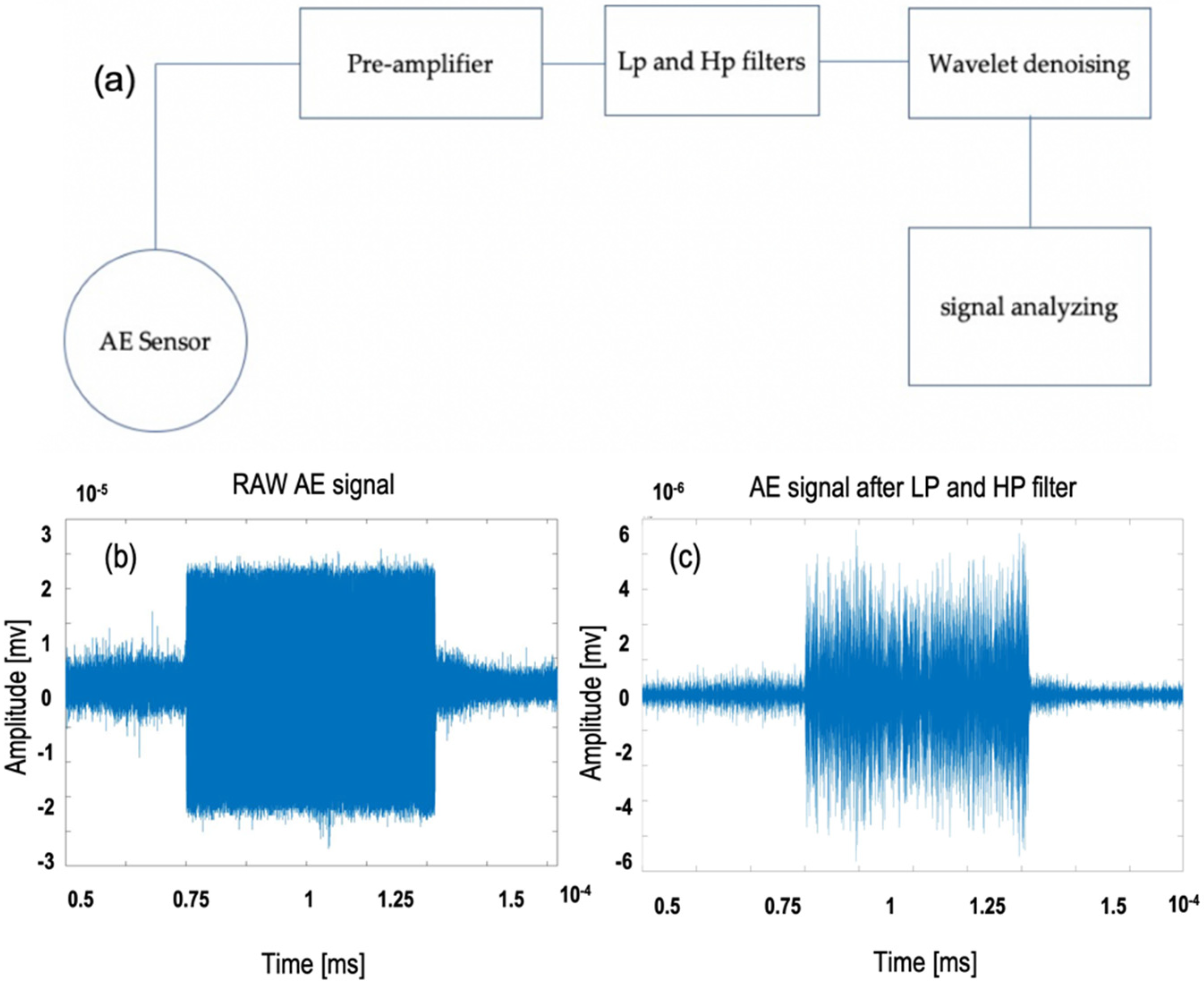
In the grinding process, the AE signals, produced by grains scratching the workpiece, are weak, which can be masked in the noises generated by the electronic device, grinding fluid impact, bond extrusion, and other sources. To process the signals first, the AE signal fed through pre-amplifier, and then, the raw amplified AE signals were subjected to further processing and recording. AE signals were then fed through low pass (LP), and high pass (HP) filters using the filter designer toolbox in MATLAB to remove the high-frequency noise components (induced by electric sparks) and low-frequency noise components to avoid aliasing. The cut-off frequency for the LP and HP filters was designed between 150 kHz and 500 kHz [
19]. Different rates for the cut-off frequency was used to avoid noisy data; nevertheless, the best cut-off frequency was chosen with the mentioned rate.
Figure 2a shows the procedure of filtering AE signals throughout the processing, (b) shows the raw AE signal before, and (c) after applying the LP and HP filters.
The manifestation of AE signal spikes at the entry and exit edges of the workpiece is a crucial problem, needing to be filtered and removed. These spikes are particularly noticeable in surface grinding [
19,
20]. To prepare the AE signal for the training model, this part of the AE signal needs to be removed. In order to use the AE signals and grinding parameters for machine learning, it is crucial to have accurate data as input. According to the literature review, the root mean square (RMS) value of the AE signals is a suitable parameter to monitor the grinding process. For accurate monitoring of the grinding process, it is essential to efficiently and effectively denoise the AE signals and keep the useful AE signals generated by abrasive grains [
21]. Zhou et al. [
21] showed in their experiments that an optimal way of denoising AE signals is utilizing empirical mode decomposed wavelet threshold. They used the signal to residual noise ratio (SRNR) and the RMS error (RMSE), as two important evaluation parameters. They tested several methods for denoising the AE signals and found that the empirical mode decomposition (EMD)-wavelet threshold is an ideal method for denoising AE signals.
The main characteristic of wavelet analysis is to extract information from the original signal by decomposing it into a group of approaches (lower frequency) and details (higher frequency), distributed over different frequency bandwidths. In this analysis, the discrete wavelet transformation (DWT) algorithm of MATLABs wavelet toolbox was used to decompose the signal into six levels. The DWT distributes the original AE signal into lower and higher frequency bands. The lower frequency band serves as an input signal for the next decomposition level; the information of the higher frequency signal is coded into a detail coefficient of the signal. These coefficients represent the degree of similarity between wavelet function and signal pattern. The total energy of the respected signal is preserved in this transformation. Therefore, band energy can be computed by integrating the square of the decomposed signal corresponding to a particular frequency band with respect to the time [
22]. Different values for wavelet denoising parameters were considered. Among all the applied parameters for denoising the AE signals, the parameters which gave the best results for denoising the AE signals and fitted all the AE signals were applied in the wavelet toolbox. The following setting has been applied to the wavelet denoising toolbox in MATLAB are. The wavelet type was set to db and number 4. The level was set to 6 with a soft universal threshold. In the universal threshold let assume that at a certain level of wavelet decomposition, the number of wavelet coefficient is x. Then the universal threshold would be:
). After decomposing the signal and omitting the noises, the signal was reconstructed.
Figure 3 shows the AE signals before and after denoising using the mentioned method.
The raw signal forms are continuous and sharply fluctuate during the grinding process. The amplitude of raw signal increases according to the number of machined workpieces, but, due to the similarity in these signals, it is not always easy to distinguish whether the grinding state is stable or unstable. Therefore, other analytic parameters are needed to identify the grinding state. Kwak and Ha [
23] claimed that the peak value of the RMS signal is sensitive to the grinding state. Therefore, RMS was used in this study for training the NN.
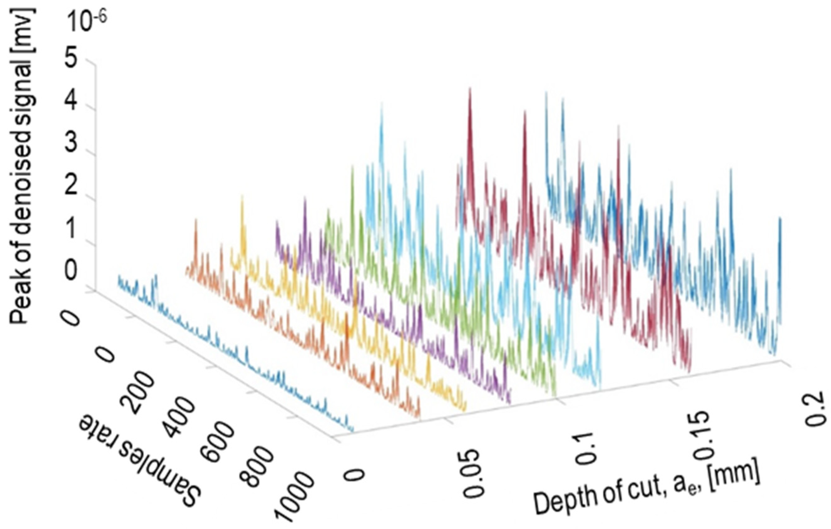
By taking into consideration that the AE signals typically have a big size (consisting of a massive amount of data), it is crucial for monitoring and building the NN to reduce the size of the data. Finding peaks of the AE signals is an approach that can reduce the size of the AE signals for the further computational process, also keeping the main information of the signals that are required for the process. To have a better view of how AE signals vary with the depth of cut, the filtered AE signal versus different depth of cut at the feed rate of 1000 mm/min, and the cutting speed of 20 m/s was plotted (
Figure 4). Increasing the depth of cut from 10 μm to 200 μm increased the AE-amplitude significantly.
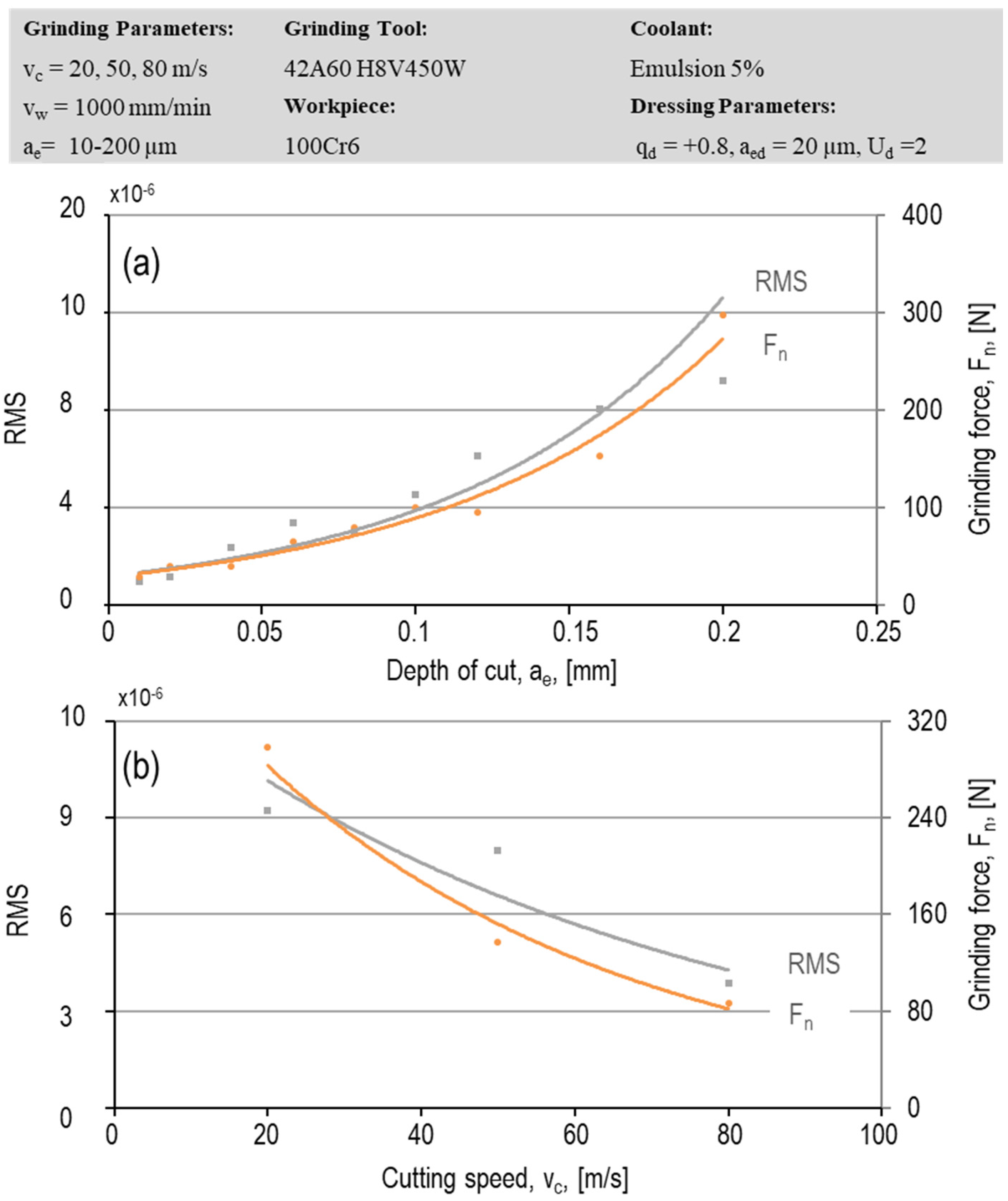
The proportion of the RMS of AE signals with the grinding forces versus depth of cut and cutting speed is also illustrated in
Figure 5a,b. These signals were collected and filtered via the first AE sensor attached to the end of the workpiece. Both a larger depth of cut and a lower cutting speed, increase the chip thickness, meaning a higher share of cutting in the process—generating higher AE signals in the grinding process, which was recorded by the AE sensor attached to the workpiece. The figure shows that increasing the normal grinding forces as a result of higher depth of cut and lower cutting speed, generated higher RMS value for AE signals—concluding a direct relationship between the grinding forces and generated AE signals during the grinding process. This capability can be used in the modeling process to predict and monitor the grinding forces and surface roughness while grinding different kind of materials.
4. Modeling
The proper design for the artificial neural network (ANN) was selected through exhaustive testing of NNs. This claim would be fulfilled by changing the number of hidden layers and the number of neurons in the hidden layer in different types of suggested ANNs. Choosing the proper training algorithm is crucial for training data for the NN. It should be considered that the low number of neurons in the hidden layer may cause a high sum square error (SSE) during the training, and the number of neurons should rise to the point that sum square errors (SSE) becomes stable. However, the SSE can be fluctuated and even be increased by raising the number of neurons. Thus, it was necessary to look after an increasing number of neurons in the feedforward NN, which was chosen for this project. The number of hidden layer neurons is typically found with trial and error approach. A routine that utilizes a feedforward Bayesian backpropagation algorithm was used to develop the model, as it has widely been used by other researchers, and it was observed that the feedforward NN algorithm gave the most reliable results [
24].
The Bayesian regularization gives a smoothness between input and output pairs with a true underlying function, which is achievable by keeping the weights small with an acceptable distribution within the neural network. The Bayesian method constrains the size of weights by adding additional terms to the objective function
F as:
where
V shows the sum of squared errors,
W is the sum of squares of the weights,
and
define objective function parameters. It is assumed in the network that the weights and biases are random variables and have specific distributions. The Bayesian method is considered to be the most appropriate technique for constructing non-linear functions between several inputs (in this case, such as feed rate and AE signal), and one or more corresponding outputs such as surface roughness [
24].
The backpropagation network typically has an input layer, an output layer, and at least one hidden layer, with each layer fully connected to the succeeding layer. During training the network, the information is also propagated back through the network and used to update the connection weights. The following expressions give the fundamental relationships used for this analysis [
25]:
is the current output state of the
qth neuron in layers,
shows the weight on the connection joining the
pth neuron in layer s-1 to the
qth neuron in layers, and
espreses weighted summation of inputs to the
qth neuron in layer s.
A backpropagation element, therefore, propagates its inputs as:
The MATLAB ANN toolbox was used for updating the value of weights and biases of the algorithm. Networks with different architecture were trained for a fixed number of cycles, and were tested using a set of input and output parameters. Linear activation functions were utilized in the output layer. The sigmoid function used in the hidden layer and input data are normalized in the range of [−1, 1] which is shown in the following equation:
The whole experimental data were divided into three different sets namely; training, validation, and test sets. The NN was trained using the training data and the during the training was validated using validation data to avoid overfittings. After training the NN was tested using the test data. The training data did not use for testing.
5. Results and Discussion
In the ANN modeling, 80 percent of the data were chosen for the training, 10 percent for validation, and 10 percent for testing of the network. As input data, the matrix consists of the peaks value of denoised AE, peaks value of the RMS of the denoised were used, and in order to give better bios to the inputs, the grinding parameters (depth of cut, cutting speed, and feed rate) also were used. However, the output data was different in various tasks; for instance, in the following ANN, the output was set to the surface roughness Ra. Due to reaching an optimal number of hidden layers, a different number of a hidden layer with a different number of neurons has been chosen. The best results were achieved with a feedforward NN with Bayesian backpropagation including two hidden layers (first hidden layer with 20 neurons and the second hidden layer with 15 neurons) and one output layer with 1 neuron.
5.1. Surface Roughness
The NN was first trained with the input data in second category, including both the AE signals and the grinding parameters, i.e., cutting speed, feed rate, and depth of cut.
Figure 6 shows the obtained results for the training of the NN to predict the surface roughness Ra. The following regression plots represent the network outputs with respect to targets for training, validation, and test sets. For an ideal fit, the data should fall along a 45-degree line, where the network outputs are equivalent to the targets. The fit was reasonably good for all data sets, with R (tangent of the slope degree of R) values in each case of 0.93 or above. Even though the Bayesian algorithm, in comparison to the Levenberg-Marquardt algorithm, needs more time for a training algorithm, the results of the Bayesian algorithm was considerably more impressive. The Bayesian backpropagation is slower because it uses the Gauss-Newton approximation to the Hessian matrix, which can be conveniently executed inside the framework of the Levenberg–Marquardt algorithm for building and training the network.
Although the performance of the regression network in the earlier and posterior steps was quite good, the noticeable results were achieved at the sixth attempt. As can be seen in
Figure 6, all the phases have a perfect slope, which shows that the NN can predict precisely the surface roughness in the term of Ra. The training phase has an R of 0.9767, which shows that all data are trained sufficiently. After the training, the trained model was tested with 10 percent of the data, showing the test has a significant R of 0.97249. The R-value of the regression model shows the capability to predict the surface roughness via ANNs.
Figure 7a shows the trend of the NN learning process. It can be seen in the figure that at the beginning of the learning process, the mean square error is high, and the model corrects itself continuously until getting a steady situation. It is also clear that all stages, including training and testing, are approximately in the same order. The best performance of the validation occurred at epoch 136, with MSE 0.011378. An epoch defines one training cycle through the whole inputs, which is different from iterations (the number of batches or steps through the data for training data, needed for finalizing one epoch). To train a neural network, more than a few epochs are generally needed. The higher number of epochs does not guarantee a better learning process, since the danger of overfitting with high number of epochs is high.
Figure 7b represents the error histogram with 20 bins (number of vertical bars), which is calculated as the difference between the targets of the NNs and the actual outputs.
The error graph also shows that most of the errors in all stages are around the middle of the error histogram, which validates the training stage. The best train result for this network was achieved in the seventh attempt. In this try, the R of the training and testing are comparatively pleasant. In some cases, changing the number of hidden layers can improve the precision of the training phase, but as it was decided to keep all have the same method (NN) for the whole process, it was decided to have the same ANNs parameters for all the data. For the target R = 0.98189 and for the training R = 0.96254. In both cases, R values were acceptable. The best performance of the validation occurred in the epoch 72, with an MSE of 0.69851. The same NN was also trained with the first input category, including just the grinding parameters. The model could be trained with acceptable accuracy of R = 0.95; however, the testing error was relatively higher than the second category (R = 0.85 compared to R = 0.98 for category two in
Figure 6). The results indicate that using cheap and easy AE signals as an input for the modeling of the surface roughness can increase the accuracy of the prediction. All predicted and experimental data for both categories are gathered in
Figure 8 for the surface roughness of Ra and Rz. The fluctuations in the surface roughness values are because of different grinding parameter sets, which resulted in different surface roughness values. The result shows that the NN could precisely predict the surface roughness with the accuracy of 99 and 97 percent for Ra and Rz, respectively when using the date set two (
Figure 8b), which is more accurate than the model trained with the input data in the category number one.
5.2. Grinding Forces
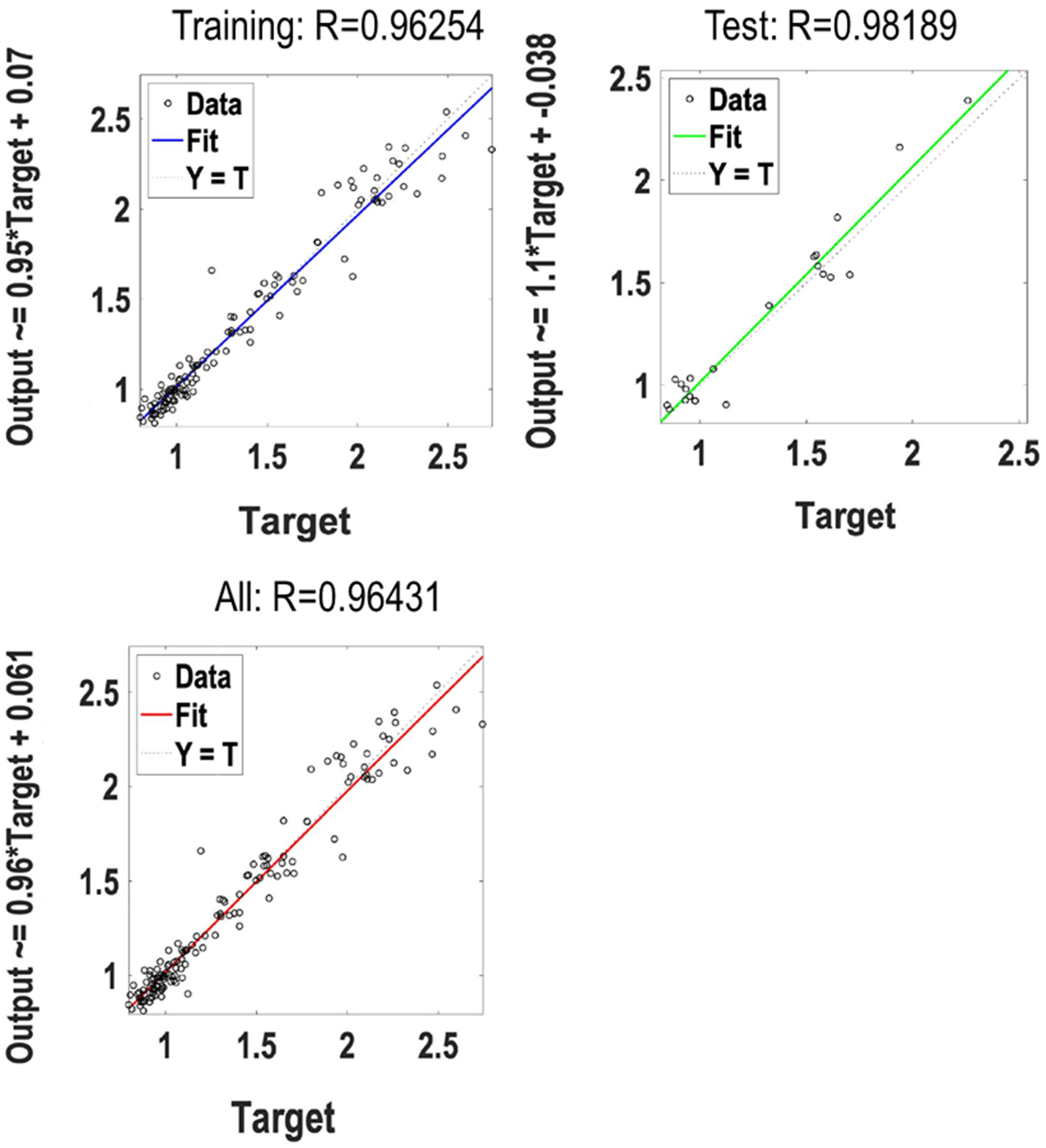
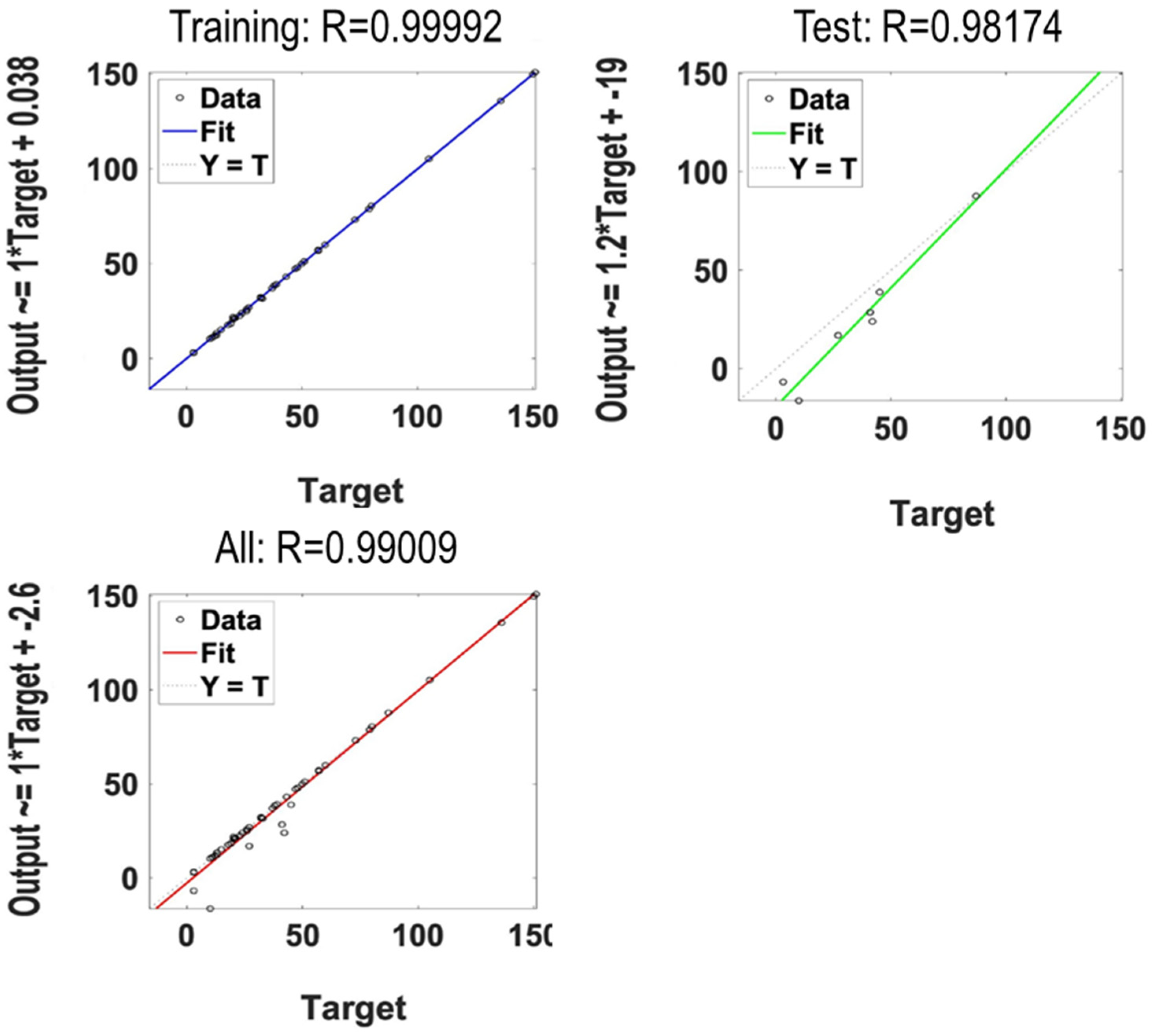
A NN was also trained for predicting the tangential and normal grinding forces with both input sets. The R values for predicting the tangential grinding forces are shown in
Figure 9 for the second category. The R-value for all three-phase, test (0.9817), training (0.9999), and target (0.99) shown an accurate prediction for the grinding forces with the use of AE signals. The same NN was also trained with the first input set (only the grinding parameters). In contrast to the surface roughness, where the trained model with the first data set could predict the surface roughness with an acceptable error, the model was not able to predict the grinding forces with high accuracy (R = 0.76 for both normal and tangential forces).
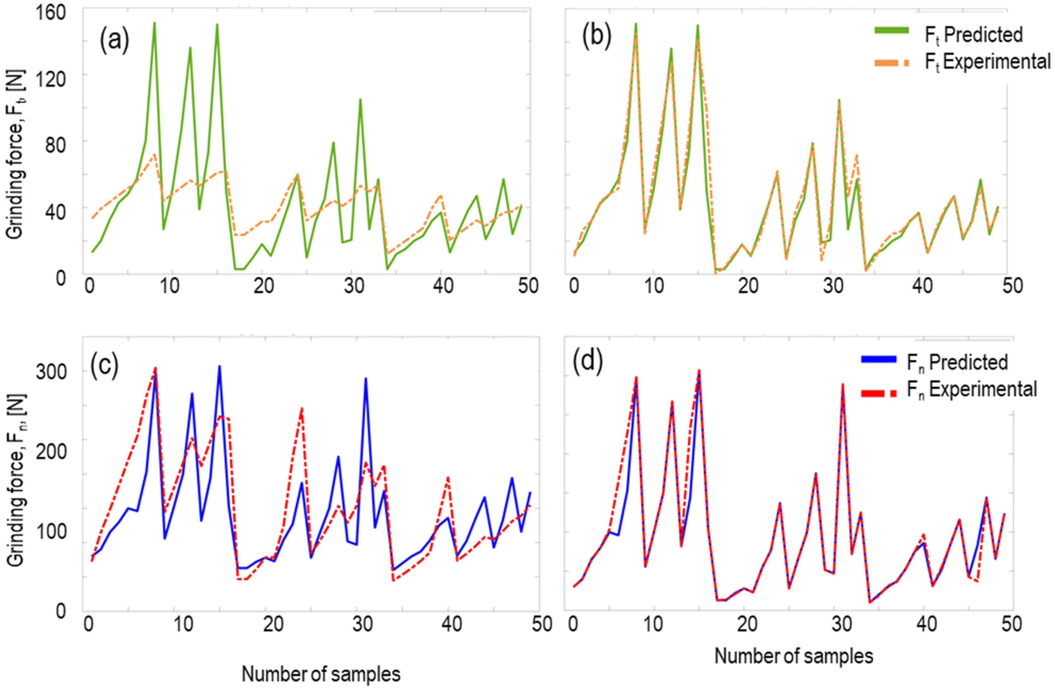
This proves that just adding the AE signal to the model as an input can increase the accuracy of the prediction model significantly. This can be more precisely seen in
Figure 10, where the results of predicted and actual values of the grinding forces are compared in both cases (
Figure 10a first input set and
Figure 10b second input set). The fluctuations of the grinding forces in
Figure 10 are as a result of different grinding parameter sets caused in grinding forces changes. The predicted grinding forces as well as the experimental results are shown in
Figure 10.
The predicted forces are in good agreement with the experimental one (with high accuracy of about 99 percent) in the case of using AE signals (
Figure 10b,d). Eliminating the AE signals from the inputs caused an increase in the uncertainty of the training phase. However, the NN was trained with an R-value of 0.76, but the prediction contained high errors, which can be clearly seen in
Figure 10a,c, where, in some cases, the prediction error exceeds 100 percent.
Figure 9 and
Figure 10 illustrate the capability of AE signals in process monitoring and how versatile it can be in the case of its usage for NN.
The result of this work shows that AE signals have a high potential to predict surface roughness and grinning forces with high accuracy. However, this should be considered that these results are limited to a specific material (100Cr6), utilized grinding tool, coolant and the grinding condition. The NN could give a very high accuracy compared to the FEM and numerical models, since they generally propose the ability of high complex non-linear models and interactions than conventional modeling procedures. Adding the AE signals as an input to the modeling process could increase the reliability of the predicted data. However, the effect of the training rate is still vague. A total of 80 percent of data were used to train the NN. In the case of surface roughness, 120 from 150 inputs were used for the training phase, which, during testing the NN, showed a highly accurate prediction. In the next step, just 30 presents of whole data were chosen randomly to train another NN, and the rest were chosen for testing. The result is presented in
Figure 11. The figure shows that, although the training rate was reduced to 30 percent, the model could predict both Ra and Rz values with high accuracies. The surface roughness of Ra could be predicted with R = 0.82 for a training rate of 30, compared to a training rate of 80 with R = 0.98. The surface roughness of Rz could be predicted with R = 0.96 for a training rate of 30, compared to the training rate of 80 with R = 0.97.


