Article

The Basics of Time-Domain-Based Milling Stability Prediction Using Frequency Response Function

1
MTA-BME Lendület Machine Tool Vibration Research Group, Department of Applied Mechanics, Budapest University of Technology and Economics, Muegyetem rkp. 3, H1111 Budapest, Hungary
2
Dynamics & Control, Ideko, Elgoibar, E20870 Basque Country, Spain
*
Author to whom correspondence should be addressed.
J. Manuf. Mater. Process. 2020, 4(3), 72; https://doi.org/10.3390/jmmp4030072
Submission received: 8 June 2020 / Revised: 12 July 2020 / Accepted: 14 July 2020 / Published: 16 July 2020
(This article belongs to the Special Issue Machine Tool Dynamics)

Abstract

:
This study presents the fundamentals of the usage of frequency response functions (FRF) directly in time-domain-based methods. The methodology intends to combine the advantages of frequency- and time-domain-based techniques to determine the stability of stationary solutions of a given milling process. This is achieved by applying the so-called impulse dynamic subspace (IDS) method, with which the impulse response function (IRF) can be disassembled to separated singular IRFs that form the basis of the used transformation. Knowing the IDS state, the linear stability boundaries can be constructed and a measure of stability can be determined using the Floquet multipliers via the semidiscretization method (SDM). This step has a huge importance in parameter optimization where the multipliers can be used as objective functions, which is hardly achievable using frequency-domain-based methods. Here we present the basic idea of utilizing the IDS method and analyze its convergence properties.

1. Introduction

Chatter vibrations belong to the main productivity limiting factors in a wide variety of machining processes such as turning, milling, or grinding. The regenerative effect, due to which the cutting edge cuts the wavy surface left in the previous pass, is the phenomenon that can give rise to this kind of self-excited vibration under certain cutting parameters. The large amplitude vibrations reached under unstable cutting provoke poor surface quality and can be harmful for both the cutting tool and the machine components.
Accordingly, the mathematical modeling of the chatter phenomenon, and more specifically, the stability analysis of the machining process, is of paramount importance in the industry and has been the object of several studies in the last decades. The stability lobe diagram (SLD), first introduced by Tobias [1], depicts the stable regions for the spindle speed-depth of cut parameter space, has been proven to be a powerful tool for chatter-free process planning. The dynamics of the cutting process subdued to regenerative effect can be described by delay differential equations (DDE), which consider the effect of both the present and the past solutions [2]. In the case of milling, the inherently time-periodic cutting force causes two effects: on the one hand, it introduces a parametric excitation to the dynamical system, which, coupled with the regenerative effect, results in a time-periodic DDE. On the other hand, the time-periodic force induces an unavoidable periodic stationary solution that determines the surface quality even for the stable case. Mathematically, chatter refers to the instability of the stationary time-periodic solution, which physically manifests as a large amplitude limiting oscillation due to the so-called fly-over effect [3,4,5].
The stability of the stationary solution of the time-periodic DDE’s arising in milling processes has been studied by means of several different approaches, commonly classified in two groups: time- and frequency-domain methods. Among the frequency-domain methods, the zeroth-order approximation (ZOA [6]), which neglects the interrupted nature of the milling process, is a very fast method for stability analysis for large immersion processes, where the parametric excitation is negligible. If the interrupted nature of the process is more pronounced, the so-called multi-frequency (MF [7,8,9,10,11]) solution should be applied. With the application of Hill’s infinite determinant, frequency domain methods parametrically provide the critical “D”-curves that depict the (non-hyperbolic) stability limit in the spindle speed-depth of cut parameter space. However, frequency-domain methods are not capable of providing a quantitative indicator of the stability for a certain cutting parameter set that somehow describes the “distance” from the stability boundary, which is commonly needed for stability-based optimization algorithms.
Alternatively to frequency-domain methods, time-domain methods—such as the semidiscretization method (SDM [12,13,14]), full-discretization [15], temporal finite element analysis (TFEA, [16]), pseudospectral collocation [17], or pseudospectral tau [18] methods—can be applied, among others. Time-domain methods provide the Floquet multipliers [19] for combinations of the spindle speed and the depth of cut over a given or fractal mesh [20]. The magnitude of the critical Floquet multiplier can not only be used for constructing the SLDs, but also provides a robust “measure” of the stability, which can be used for process optimization purposes [21].
Aside from how the stability properties are provided, another critical aspect is how the dynamics of the system are defined. Frequency-domain methods can directly work with the measured frequency response functions (FRFs), whereas time-domain methods require the time-domain representation of the system dynamics, given either in the Cartesian space with the system matrices or—more conveniently—in modal space by means of the so-called modal parameters. While switching from time- to frequency-domain representation by means of theoretical modal analysis is straightforward [22], obtaining the modal parameters for a given sampled FRF or a set of FRFs requires a modal parameter fitting [23], which can hardly be automated and whose accuracy relies on the fitting method and the experience of the person who carries it out.
In the last years, the rapid advances of the industry in terms of sensors and monitoring software have moved the machine tool industry towards new “smart” machine designs that can not only monitor the actual condition of the machine, but also predict its in-service behavior. Among others, self-characterization of the machine tool dynamic behavior has gained increasing interest among the manufacturers, who take advantage of the built-in shakers and accelerometers installed on the machine tool for active damping proposes for unmanned measuring of the FRFs over the entire workspace. The next step is the feeding of the dynamic behavior to stability analysis software for prediction or process optimization purposes. However, as it was previously mentioned, the highly robust time-domain methods cannot directly deal with the measured FRFs, and require an alternative approach for a fully automated stability prediction.
In this paper, a milling stability model based on semidiscretization for direct usage of sampled frequency response functions is presented. To this end, an abstract impulse dynamic subspace (IDS [24]) based on the singular value decomposition (SVD) is introduced for time-domain representation of the system dynamics, avoiding manual fitting of modal parameters. Then, the asymptotic stability of the system is derived by means of semidiscretization, whose results are compared to the equivalent modal parameter-described system. Later, the newly developed IDS-based SDM is compared with literature-based measurements from the work in [25], in which fine quality experimental data is collected for tailored 1DOF milling processes.

2. Model and Methods

The proposed methodology is a general dynamical description that can be used for many other dynamical systems, not only for the one originated from machining problems. Considering that this representation is more complex and atypical than the conventional modal analysis-based description, the mechanical model is kept as simple as it is possible. We chose milling processes since these processes are both time periodic and regenerative [26], and, at the same time, provide a nice example to have both Hopf (H) and period doubling (flip, PD) type instabilities [27].

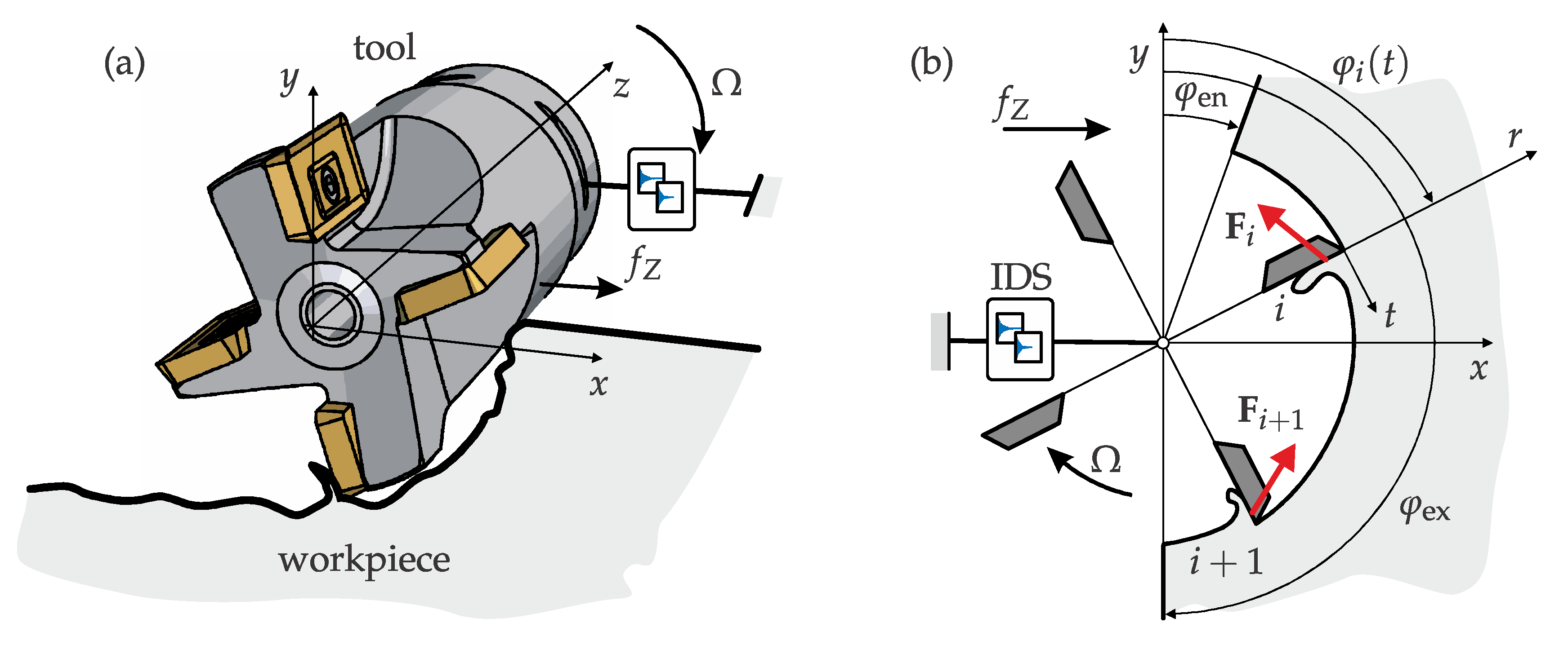
2.1. Regenerative Milling Model

Here, for the sake of simplicity, a 1D milling model is used (see Figure 1a) considering a single vibration mode in the x (feed) direction. The cylindrical cutter with diameter D has lead angle κ = 90 deg , Z number of teeth, and features zero helix flutes and regular pitch distribution. The cutter rotates at a constant angular velocity Ω and moves along the x direction with a feed per tooth f Z . Thus, the specific cutting force with linear characteristics can be considered in the tangential, radial ( t r ) plane as
f t r , i ( t , x ( t ) , x ( t τ ) ) = K e K c h i ( t , x ( t ) , x ( t τ ) ) ,
where K e = col ( K e , t , K e , r ) and K c = col ( K c , t , K c , r ) are, respectively, the edge and cutting coefficients resulting from the linear regression of the experimentally measured mean cutting forces [26]. τ is the regenerative delay, which equals the tooth passing period T Z = 2 π / ( Ω Z ) in this simple case. The momentary chip thickness is defined as
h i ( t , x ( t ) , x ( t τ ) ) ( f Z + x ( t ) x ( t τ ) ) sin φ i ( t ) ,
where φ i ( t ) = Ω t + 2 π ( i 1 ) / Z refers to the angular position of the tooth i as depicted in Figure 1b. The total cutting force projected in the flexible x direction is then computed as the sum of the contribution of all the Z teeth in the entire depth of cut a as
F x ( t , x ( t ) , x ( t τ ) ) = a i = 1 Z g i ( t ) K e , t + K c , t h i ( t , x ( t ) , x ( t τ ) ) cos φ i ( t ) + K e , r + K c , r h i ( t , x ( t ) , x ( t τ ) ) sin φ i ( t ) .
where g i ( t ) stands for the screen function, which determines whether the tooth is in or out of cut. The total cutting force can be split in a time-periodic stationary term F x , 0 ( t ) = F x , 0 ( t + T Z ) and a state-dependent variational term Δ F x ( t ) : = Δ F x ( t , x ( t ) , x ( t τ ) ) as
F x ( t ) : = F x ( t , x ( t ) , x ( t τ ) ) = F x , 0 ( t ) + Δ F x ( t , x ( t ) , x ( t τ ) ) = F x , 0 ( t ) + C ( t ) ( x ( t ) x ( t τ ) ) ,
where
F x , 0 ( t ) = a i = 1 Z g i ( t ) K e , t + K c , t f Z sin φ i ( t ) cos φ i ( t ) + K e , r + K c , r f Z sin φ i ( t ) ) sin φ i ( t )
and
C ( t ) = a i = 1 Z g i ( t ) K c , t sin φ i ( t ) cos φ i ( t ) + K c , r sin 2 φ i ( t ) .
The stationary term in (4) induces an unavoidable stationary solution, which physically manifests as a forced vibration even for the stable case, and that results in marks on the machined surface. The latter state-dependent term—commonly known as dynamic force or regenerative force—can eventually lead to unstable behavior under certain cutting parameters, giving rise to the aforementioned chatter vibration.

2.2. IDS-Based Dynamics And Stability

The governing dynamics of milling processes can be modeled either in modal or Cartesian space. In the industrial use, modal description is preferred, as it is closely related to the parameters that can be determined using experimental modal analysis and fitting techniques [28]. However, the result of the fitting strongly depends on the level of the user experience, directly influencing the stability calculation. The manual nature and the use of expensive expert hours makes the parameter-based methods highly impractical from an automation point of view. A more self-reliant method is needed in the industry, where the sensitivity of the manufacturing process towards the variation of technological parameters is of major interest especially for optimization purposes. The impulse dynamic subspace (IDS) description serves as a good option to determine the process behavior by combining its fair accuracy and its possible self-reliant application on measured FRFs.
The structural dynamics can be described by the continuous impulse response function (IRF, h ( t ) ( m / ( N s ) ), derived from experimental FRFs ( H ( ω ) ( m / N ) ) by means of the inverse Fourier transform as
h ( θ ) = F 1 H ( ω ) ( θ ) .
Accordingly, the integral form of the dynamical system can be represented as
x t ( θ ) : = x ( t + θ ) = 0 T G ( θ , ϑ ) F x ( t ϑ ) d ϑ + 0 θ h ( θ ϑ ) F x + ( t + ϑ ) d ϑ ,
where G ( θ , ϑ ) = h ( θ + ϑ ) is the Green function defined over the interval θ [ 0 , T ] . The finite length T of the measured IRF is directly related to the frequency resolution δ f of the FRF, since T = 1 / δ f . The first term of (8) actually corresponds to the homogeneous dynamics as a result of initial forcing via the Green function G. In this manner, as an alternative to the usually used initial conditions (IC’s), the system reaches its initial state at time t by the (initial) past force pattern described by F x . This hypothetical force evolution pushes the system to the opening state at t, afterwards it gradually behaves as a forced (excited) dynamic system described by the second term of (8). The present (excitation) force F x + operates via the IRF, which results in the time periodic stationary forced vibration combined with the transient response of the system to zero IC, without considering the state dependency, e.g., in (3). In milling, (8) has a periodic (stationary) solution, x ¯ ( t ) = x ¯ ( t + T Z ) , due to (4) that can be determined, e.g., by harmonic balance or considering the long term behavior of the second term of (8). It can be defined for a time-period T Z after the vanishing transient response at T t ( T t : = M T Z , where M N + to keep the phase) as
x ¯ 0 ( θ ) x ¯ T Z ( θ ) = 0 T t + T Z h ( θ + T t ϑ ) F x ( ϑ , x ¯ 0 ( ϑ mod T Z ) , x ¯ 0 ( ( ϑ τ ) mod T Z ) ) d ϑ ,
satisfying the causality condition h ( θ 0 ) = 0 . Around the stationary solution x ¯ ( t ) , a perturbation u ( t ) is considered in the form x : = x ¯ + u . Consequently, the perturbed motion is described by the following so-called variational system that is given as
u t ( θ ) = 0 T G ( θ , ϑ ) Δ F u ( t ϑ ) d ϑ + 0 θ h ( θ ϑ ) Δ F x ( t + ϑ , u t + ϑ ( 0 ) , u t + ϑ ( τ ) ) d ϑ .
The measured FRF is given with a certain frequency resolution δ f due to the digital sampling, which determines the length of the IRF as T = 1 / δ f . Therefore, the solution is defined over the time mesh t j = j δ t ( δ t = δ θ = 1 / f max , j = 0 , 1 , , N 1 , f max = ( N / 2 1 ) δ f ) as
u T ( t ) = G Δ F T ( t ) + H C ( t ) ( u T ( t τ ) u T ( t ) ) ,
where Δ F T ( t ) = col k Δ F x ( t ( k 1 ) δ θ ) , C ( t ) = diag k C ( t + ( k 1 ) δ θ ) , while u T ( t ) = col k u ( t + ( k 1 ) δ θ ) . Similarly, the IRF is also considered in its sampled form as h k = h ( ( k 1 ) δ θ ) . The Toeplitz and Hankel representations of the forced IRF and the Green function are given as
H = h 0 0 0 h 1 h 0 0 h N 1 h N 2 h 0 and G = h 0 h 1 h N 1 h 1 h 2 h N h N 1 h N h 2 ( N 1 ) ,
respectively. Note that G is theoretically a full matrix, but h k = 0 if k > N 1 due to practical reasons.

2.2.1. Impulse Dynamic Subspace (IDS) Transformation

Instead of the usual modal parameter-based description of the system, the homogeneous dynamics is constructed over its singular impulse response characteristics [24], defined by SVD on the Hankel representation of the Green function (12):
u T ( t ) = G Δ F T ( t ) V Σ W H Δ F T ( t ) .
It is known that the SVD gives the dominant principle directions with respect to their “stored energy” or, based on receptance IRF, with respect to their compliance. The singular values are given in Σ = diag k σ k , such that σ 1 > σ 2 > > σ k > > σ N . Many of the σ k singular values almost vanish, which means that these vanishing directions have little influence in (13), thus truncation can be performed. Using n < N dimensional truncation, the new reduced set of singular IRFs can be defined as V n = [ v 1 v 2 v 3 v n ] . Knowing that V n is an orthonormal set due to its very definition in (13), a new abstract state p ( t ) = col k p k ( t ) can be defined as
p ( t ) = V n H u T ( t ) Σ n W n H Δ F T ( t ) u T ( t ) = V n p ( t ) .
By using the continuous description, like in (8), the solution and its derivative can be deduced similarly to (14):
u ( t + θ ) = V n ( θ ) p ( t ) u ˙ ( t + θ ) = V n ( θ ) p ˙ ( t ) V n ( θ ) p ( t ) ,
where a ˙ = d a / d t and a = d a / d θ . Thus, the system matrix can be derived using the product of the singular IRFs with its derivatives as
p ˙ ( t ) = V n H V n p ( t ) .
The derivative of the singular IRFs, V n , can be determined using the sampled representation G of G ( θ , ϑ ) , and consequently
V n = G W n Σ n 1 .
Therefore, the solution for the initial forcing (IF) is
p IF , l ( t ) = e V n H V n ( t t l ) b ,
based on (16) from a given initial time t l .
The methodology how the system matrix is introduced in (16) can be a base of an alternative modal analysis technique. The eigenvalues of V n H V n are actually the poles that directly define the natural frequency and damping factor shown in [24].

2.2.2. Stability Prediction by Semidiscretization Method

The delayed nature of the regenerative milling process [29,30] requires discretization on the past motion of the tool that directly leads to a possible semidiscretization description, where the stationary forcing plays an important role.
For this purpose, another new time sampling Δ t = D δ t ( D N + ) is needed to define a mesh t l = t j + ( l 1 ) Δ t , as the time step δ t is likely too small to construct an efficient numerical method (SDM). Afterwards, r = τ Δ θ 1 2 intervals ( Δ t = Δ θ ) are defined for simplicity with τ : = T Z (regular cutter). The second term of (11) describes the forced solution p F 0 ( t ) with its transient for zero ICs considering constant (zero-order hold) actual and delayed states measured to t l . Taking into account the transformation in (14), the forcing solution combined with the zero transient solution (F0) is given in the time interval t [ t l , t l + 1 ] as
p F 0 , l ( t ) = δ t V n H H C ( t ) V n ( p l , τ p l ) ,
where p l = p ( t l ) and p l , τ p l r . The solution in t [ t l , t l + 1 ] in the form p l ( t ) = p IF , l ( t ) + p F 0 , l ( t ) can be expressed as
p l ( t ) = e V n H V n ( t t l ) b + δ t V n H H C ( t ) V n ( p l , τ p l ) .
Considering that only the initial forcing (IF) term adopts to nonzero ICs, p h , l ( t l ) = p l , the next time step has the following form,
p l + 1 = e V n H V n Δ t p l + δ t V n H H D C l , D V n , D ( p l , τ p l ) ,
where H D and V n , D are truncated matrices related to the integer number ratio D between Δ t and δ t .
The exponential expression of the initial forcing can be obtained by shifting the IDS by Δ t as shown in [24]. This can be defined by a shift matrix S , resulting in
p l + 1 = V n H S V n p l + δ t V n H H D C l , D V n , D ( p l , τ p l ) .
A discretized state, z l = col k ( p l , p l 1 , p l 2 , , p l r ) , can be introduced by which both (21) and (22) can be transformed to a map as
z l + 1 = B 0 z l .
The map in (23) is reapplied successively over the time period T Z in order to have the so-called transition matrix Φ
z l + r = Φ z l with Φ = B r 1 B r 2 , B 0 ,
where N SDM : = r is the applied SDM scheme resolution.
The characteristic multipliers (eigenvalues) of the transition matrix directly represent the asymptotic behavior of the stationary solution x ¯ . The less than one magnitudes for all characteristic multipliers corresponds to stable stationary solution. Otherwise, x ¯ is unstable or critically stable. Thus, SLDs can be constructed based on the magnitudes of the characteristic multipliers.
In summary, the IDS description can provide a methodology, in which the step of the parameter extraction can be avoided (see flowcharts in Figure 2). This is an advantage since parameter extraction is a time consuming action, which typically needs expert interaction. The effectivity of parameter-based pure numerical algorithms, like SDM, are usually measured without considering the modal parameter extraction step, which can carry significant errors, too, depending on the complexity of the initial FRF. The proposed methodology is initiated from a corresponding IRF, which is usually originated from measured FRFs (Figure 2b). By performing an SVD on the Green function, the entire dynamical system is described using a selected set of singular IRFs V n , by determining the system matrix A = V n H V n (16) or the solution operator V n H S V n (22) for the core homogeneous (ordinary) dynamics. By choosing an appropriate time step, based on the parameters taken from the stability chart ( n ( rpm ) , a ( mm ) ), an interpolation is performed on the singular-IRF set and the corresponding forcing term can be added (16). This map actually describes the step matrix (approximated solution operator) B j ( j = 0 , 1 , , r 1 ) of the original regenerative (delayed) system, which leads to the transition matrix Φ in an iterative manner.

3. Results and Discussion

In this chapter, we give an insight on the effectivity of the proposed method related to its convergence and its relation to the reality through an experimental case taken from the literature.

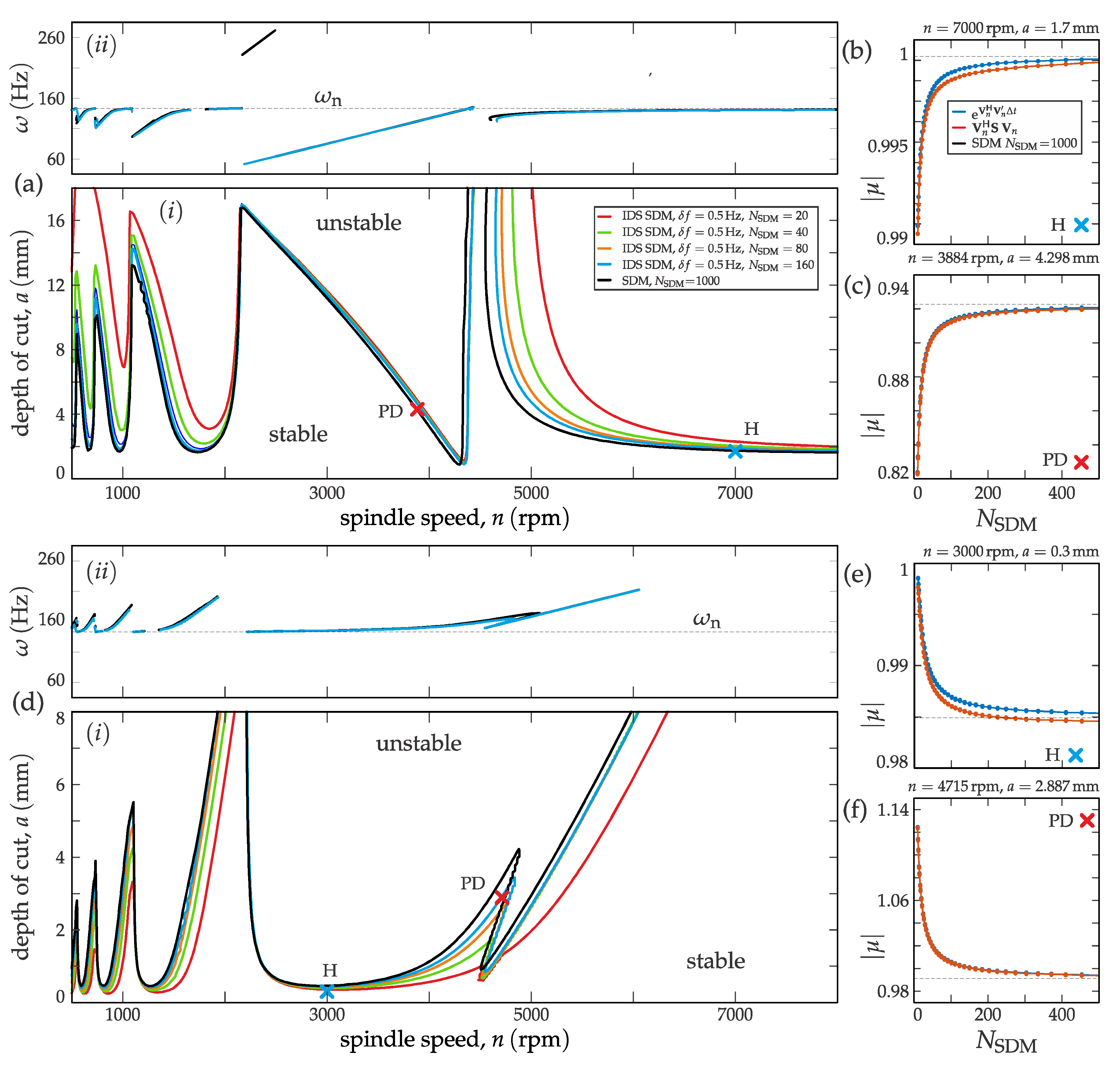
3.1. Convergence Analysis

The map presented in (24) is used for approximating the monodromy operator of the time-periodic milling system, also known as the transition matrix Φ , in order to calculate stability charts (Figure 3a,d) of the corresponding stationary solution x ¯ . A simple artificial one DOF FRF is considered from the work in [31] as the base of the calculation with relative damping ζ = 1 % , natural frequency ω n = 146.5 Hz , and stiffness k = 6.18 N / μ m . The tested processes are half immersion up/down-milling cases performed using straight fluted tool ( Z = 4 ) and material with the following cutting parameters; K c , t = 550 MPa and K c , r = 200 MPa . The presented SLDs (Figure 3a,d(i)) are constructed using the IDS originated from IRF/FRF by applying SVD on the homogeneous core of the dynamics ( G ( θ , ϑ ) at (12)). Corresponding frequencies at the stability boundaries are shown in (Figure 3a,d(ii)).
It can be seen that the solutions provided by the proposed IDS SDM converges to the known solutions, although the required resolution is higher than that for the solution constructed using the ordinary parameter-based SDM. The reason of this difference is that, in the case of IDS SDM, the parameters are the indirect result of a nested convolution using the corresponding IRF, which causes considerable numerical error. However, one can say, this error is actually embedded in the parameters, too, as parameters in the reality must be determined with some methodology, whose computation cost and error are not included in the pure parameter-based numerical methods.
As in the conventional SDM, the accuracy of the IDS SDM decreases for larger time delays, that is, for lower spindle speeds if τ ( s ) T Z ( s ) = 60 ( s / min ) Z n ( rpm ) . This phenomenon is apparent in all SLDs in Figure 3a,d(i)). The dominant vibration frequencies can be calculated using the critical characteristic multiplier and its corresponding eigenvector [32], which approaches the exact (SDM, N SDM = 1000 ) case quite well (see Figure 3a,d(ii)). In terms of Hopf-related stability loss (H), Figure 3a,d(ii)) shows the well-known behavior [33] when milling process with negative directional factor oscillates with lower, while milling process with positive directional factor oscillates with higher vibration frequencies ω than the corresponding natural frequency ω n . In the case of period-doubling (PD)-related instability, the vibration frequencies ω in (see Figure 3a,d(ii)) are located on a straight line ω ( n ) ( Hz ) = ( m / 2 ) / ( T Z ( n ) ( s ) ) Z n ( rpm ) 60 ( s / min ) (m is odd), which can be used for identifying PD related curves in the SLDs (see Figure 3(i)). The converged solution shows high discrepancy for the DM case in Figure 3a(ii)) in the range n [ 2000 , 3000 ] rpm , which is due to the relocation of dominance between different modulations of ω . In general, the convergence is better for period-doubling (flip) type (PD) of instabilities because these are more strongly related to the well-represented time-periodic nature of the milling process than to its delayed essence.
It can be seen in the convergence tests in Figure 3b,c,e,f that the system matrix-based expression ( e V n H V n Δ t ) of the map (21) is more accurately approaching the exact solution (def: original SDM [12] with N SDM = 1000 ), whereas the shifted IDS-based solution ( V n H S V n ) converges slightly off the exact solution, which is more apparent in the case of Hopf type (H) of points in Figure 3b,e.
This effect is due to the sampled nature of the original IRF assembled in the Hankel form of the Green matrix in (12). Theoretically, in continuous linear form, the shifted convolution V n H S V n V ( θ ) , V ( θ + Δ t ) is an exact representation of the matrix exponential form e V n H V n Δ t e V ( θ ) , V ( θ ) Δ t at Δ t , that is, V ( θ ) , V ( θ + Δ t ) = e V ( θ ) , V ( θ ) Δ t . This equity is formally true but truncation and sampling creates discrepancy between the two representations.

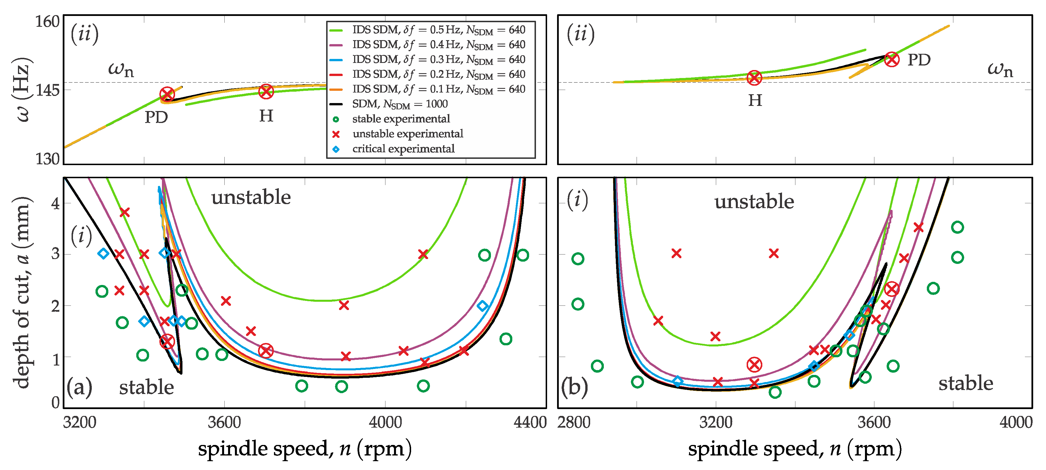
3.2. Comparing with Experiments

After having the convergence analysis, a literature example is used [25] for justifying the model in real circumstances. As the presented convergence analysis was performed in a one-DOF case, the specially tailored experiments presented in [25] provide excellent data for comparison, even though these results primarily refer to the goodness of the model rather than to the efficiency of the numerical method itself. The experiments were performed by using a special one DOF workpiece holder with dominant dynamic behavior slightly different to the one analyzed in the previous section. The experiments were carried out using a flexible aluminum ( K c , t = 550 MPa , K c , r = 200 MPa ) fixture with one dominant mode ( ω n = 146.5 Hz , ζ = 0.32 % , k = 2.18 N / ( μ m ) ) and a single fluted tool Z = 1 on up- and down-milling situations with 23.7 % radial immersion.
This literature experimental example [25] provides an excellent possibility to test the IDS SDM approach introduced in the paper. In the measurement, the authors distinguished stable (), unstable (×), and critical cases (), which gives a hint about uncertainties (see Figure 4(i)). Due to the specially designed aluminum workpiece holder, the corresponding damping is really small ζ = 0.32 % , which requires the reduction of the frequency resolution δ f to represent FRF and IRF correctly for the IDS SDM methodology. By considering the frequency difference between “peak” and “valley” in the real part of the corresponding FRF Δ ω : = ω n 1 + 2 ζ 1 2 ζ , the resolution requirement can be designed for a single-DOF viscous damped system. The results presented in Figure 3 are all calculated using δ f = 0.5 Hz resolution, leading to approximately 5 points in Δ ω ζ = 1 % = 2.93 Hz .
By decreasing the frequency resolution δ f gradually to 0.1 Hz in Figure 4(i)), the IDS SDM solutions approach exact solutions (SDM N SDM = 1000 ) approximately when δ f reaches 0.2 Hz . This actually means reaching roughly 5 sampled points in the specific “width” of the resonance ( Δ ω ζ = 0.32 % = 0.93 Hz ), which could be a requirement even for a parameter identification method to have the fairly accurate modal description. This is an important point, as this implication is not considered in the calculation load of the classical SDM. Moreover, it happens many times that low damping is not well captured in modal measurements due to the insufficient experimental frequency resolution of the FRF/signal length of the IRF used during modal experiments.
In the vibration frequency diagrams, four experimentally “unstable” measurements are indicated, for which [25] reported the so-called chatter frequency values. These are the arisen experimental dominant vibration frequencies that do not correspond to any tooth passing harmonics ( l T Z , l N ). One can realize that these frequencies take place quite close to the predicted exact frequencies (black curves in Figure 4(ii)). Furthermore, their errors are in the range of the inaccuracy of the worst approximation of the convergence analysis (green curves in Figure 4(ii)). As it was mentioned, in the case of the Hopf-related instabilities (H), these chatter frequencies arise close to the corresponding natural frequencies, while for the period doubling type stability losses (PD), the frequencies are locked with the tooth passing frequencies. Unfortunately, this effect is not that strongly apparent in the values published in [25], as the points are chosen quite close to the zone of mode interaction [34], where Hopf related frequencies can contaminate the measurement spectra.
Obviously, the IDS SDM cannot provide a better solution for the same model than the conventional SDM methodology. The difference between the model and the experiments is present for both numerical methodologies. It is clear that the IDS SDM has its own limitations due to its more signal oriented approach, but there is plenty of room for improvements. This theoretical framework can be refined by using only the spatial coordinates for delayed states [35] or/and applying the so-called implicit subspace iteration methodology [36] that will cure the size problem arisen due to the required high discretization resolution. Moreover, the nested nature of the convolutions can include more simplification possibilities that would be helpful to make the proposed method more effective. Even though it seems that low damping is problematic for the presented IDS SDM, the level of low damping in Figure 4 is quite rare in the industry for the machine-originated chatter cases, where the automated IDS SDM could exploit greater its potential. It is more important that the IDS SDM is a convergent algorithm even reaching the case depicted in Figure 4, while working fine for cases with more realistic 1 % or higher damping.

4. Conclusions

In the present contribution, the basics of a new, alternative method were presented that can be used to determine the stability properties of delayed time-periodic dynamical systems. It is shown that the so-called impulse dynamic subspace (IDS [24]) can be used for transforming the state dependent and time-periodic cutting force excitation (originated from the milling process) into convergent form. In the derivation, simple zero-order hold was used for approximating the past solution, which naturally leads to a kind of semidiscretization formalism (SDM), by which the so-called transition matrix can be compiled. After having the transition matrix, the Floquet multipliers can be determined in the usual manner. Convergence tests were performed showing that somewhat higher resolution is needed for IDS SDM than for the parameter-based conventional SDM. Although the present initial work does not solve this problem, it serves hints for possible solutions that can improve the proposed methodology. The proposed IDS methodology avoids the step of modal parameter extraction, which brought errors and computational costs that are not considered on the effectivity analysis of pure parameter-based algorithms. It is important to mention that this method can incorporate the measured IRF signal and can provide the measure of stability in the form of the magnitude of the critical eigenvalue. Satisfying these two requirements was not possible so far; however, both are indispensable for an industry-friendly method, regardless of its computational cost. The methodology described in the present work is not restricted to dynamical systems originated from machining processes. The milling process was a convenient choice to test the methodology due to its delayed (regenerative) and time-periodic nature.

Author Contributions

In this research, the base conceptualization and supervision were performed by M.Z., while further conceptualization, the methodology and software development, and the writing were performed by Z.D. M.S.-C. was partially responsible for writing—review and editing, and visualization. All authors have read and agreed to the published version of the manuscript.

Funding

This research was funded by Hungarian NKFI FK 124361.

Acknowledgments

This research work has been done under the framework of the project MIRAGED: Posicionamiento estratégico en modelos virtuales y gemelos digitales para una industria 4.0 (CER-20191001), supported by CDTI-acreditación y concesión de ayudas destinadas a centros tecnológicos de excelencia cervera.

Conflicts of Interest

The authors declare no conflict of interest.

Abbreviations

The following abbreviations are used in this manuscript.
IDSimpulse dynamic subspace
FRFfrequency response function
ZOAzeroth order approximation
MFmulti-frequency
SVDsingular value decomposition
SDMsemidiscretization method
IRFimpulse response function
ICinitial condition
IFinitial forcing
F0stationary forcing combined with zero IC transient
UMup-milling
DMdown-milling
DOFdegrees of freedom
DDEdelay-differential equation
SLDstability lobe diagram

References

  1. Tobias, S.; Fishwick, W. Theory of Regenerative Machine Tool Chatter. Engineer 1958, 205, 199–203. [Google Scholar]
  2. Stepan, G. Retarded Dynamical Systems; Longman: London, UK, 1989. [Google Scholar]
  3. Kondo, Y.; Kawano, O.; Sato, H. Behavior of Self-Excited Chatter Due to Multiple Regenerative Effect. ASME J. Manuf. Sci. Eng. 1981, 103, 324–329. [Google Scholar] [CrossRef]
  4. Tlusty, J.; Ismail, F. Basic Non-Linearity in Machining Chatter. CIRP Ann. 1981, 30, 299–304. [Google Scholar] [CrossRef]
  5. Dombovari, Z.; Barton, D.A.; Wilson, R.E.; Stepan, G. On the global dynamics of chatter in the orthogonal cuttingmodel. Int. J. Non-Linear Mech. 2010, 46, 330–338. [Google Scholar] [CrossRef] [Green Version]
  6. Altintas, Y.; Budak, E. Analytical prediction of stability lobes in milling. CIRP Ann. Manuf. Tech. 1995, 44, 357–362. [Google Scholar] [CrossRef]
  7. Minis, I.; Yanushevsky, R. A New Theoretical Approach for the Prediction of Machine Tool Chatter in Milling. ASME J. Eng. Ind. 1993, 115, 1–8. [Google Scholar] [CrossRef]
  8. Budak, E.; Altintas, Y. Analytical Prediction of Chatter Stability in Milling—Part I: General Formulation. J. Dyn. Syst. Meas. Control 1998, 120, 22–30. [Google Scholar] [CrossRef]
  9. Merdol, S.D.; Altintas, Y. Multi Frequency Solution of Chatter Stability for Low Immersion Milling. J. Manuf. Sci. Eng. 2004, 126, 459–466. [Google Scholar] [CrossRef]
  10. Zatarain, M.; Bediaga, I.; Munoa, J.; Insperger, T. Analysis of directional factors in milling: Importance of multi-frequency calculation and of the inclusion of the effect of the helix angle. Int. J. Adv. Manuf. Technol. 2010, 47, 535–542. [Google Scholar] [CrossRef]
  11. Bachrathy, D.; Stepan, G. Improved prediction of stability lobes with extended multi frequency solution. CIRP Ann. Manuf. Technol. 2013, 62, 411–414. [Google Scholar] [CrossRef]
  12. Insperger, T.; Stepan, G. Semi-discretization method for delayed systems. Int. J. Numer. Methods Eng. 2002, 55, 503–518. [Google Scholar] [CrossRef]
  13. Insperger, T.; Stepan, G. Semi-Discretization for Time-Delay Systems: Stability and Engineering Applications; Springer: New York, NY, USA, 2011. [Google Scholar]
  14. Dombovari, Z.; Munoa, J.; Stepan, G. General milling stability model for cylindrical tools. Procedia CIRP 2012, 4, 90–97. [Google Scholar] [CrossRef] [Green Version]
  15. Ding, Y.; Zhu, L.; Zhang, X.; Ding, H. A full-discretization method for prediction of milling stability. Int. J. Mach. Tools Manuf. 2010, 50, 502–509. [Google Scholar] [CrossRef]
  16. Bayly, P.; Halley, J.; Mann, B.; Davies, M. Stability of Interrupted Cutting by Temporal Finite Element Analysis. J. Manuf. Sci. Eng. 2003, 125, 220–225. [Google Scholar] [CrossRef]
  17. Breda, D.; Maset, S.; Vermiglio, R. Pseudospectral Differencing Methods for Characteristic Roots of Delay Differential Equations. SIAM J. Sci. Comput. 2005, 27, 4. [Google Scholar] [CrossRef]
  18. Lehotzky, D.; Insperger, T. A pseudospectral tau approximation for time delay systems and its comparison with other weighted residual type methods. Int. J. Numer. Meth. Eng. 2016, 108, 588–613. [Google Scholar] [CrossRef] [Green Version]
  19. Farkas, M. Periodic Motions; Springer: Berlin, Germany; New York, NY, USA, 1994. [Google Scholar]
  20. Bachrathy, D.; Stepan, G. Bisection method in higher dimensions and the efficiency number. Period. Polytech. Mech. Eng. 2011, 56, 81–86. [Google Scholar] [CrossRef] [Green Version]
  21. Stepan, G.; Hajdu, D.; Iglesias, A.; Takacs, D.; Dombovari, Z. Ultimate capability of variable pitch milling cutters. CIRP Ann. 2018, 67, 373–376. [Google Scholar] [CrossRef]
  22. Ewins, D. Modal Testing: Theory, Practice, and Applications; Research Studies Press: Boston, MA, USA, 2000. [Google Scholar]
  23. Richardson, H.M.; Formenti, D.L. Parameter estimation from frequency response measurements using rational fraction polynomials. In Proceedings of the 1st IMAC Conference, Orlando, FL, USA, 8–10 November 1982. [Google Scholar]
  24. Dombovari, Z. Dominant modal decomposition method. J. Sound Vib. 2017, 392, 56–69. [Google Scholar] [CrossRef]
  25. Mann, B.; Inspergeer, T.; Bayly, P.; Stepan, G. Stability of up-milling and down-milling, Part 2: Experimental verification. Int. J. Mach. Tools Manuf. 2003, 43, 35–40. [Google Scholar] [CrossRef] [Green Version]
  26. Altintas, Y. Manufacturing Automation: Metal Cutting Mechanics, Machine Tool Vibrations, and CNC Design; Cambridge University Press: Cambridge, UK; Cambridge, MA, USA, 2000. [Google Scholar]
  27. Szalai, R.; Stepan, G. Lobes and Lenses in the Stability Chart of Interrupted Turning. J. Comput. Nonlinear Dyn. 2006, 1, 205–212. [Google Scholar] [CrossRef]
  28. Phillips, A.; Allemang, R.J.; Brown, D.L. Autonomous Modal Parameter Estimation: Methodology. Part Ser. Conf. Proc. Soc. Exp. Mech. Ser. 2011, 3, 363–384. [Google Scholar]
  29. Stepan, G.; Szalai, R.; Mann, B.; Bayly, P.; Insperger, T.; Gradisek, J.; Goverkar, E. Nonlinear dynamics of high-speed milling—Analyses, numerics, and experiments. J. Vib. Acoust. 2005, 127, 197–203. [Google Scholar] [CrossRef]
  30. Insperger, T. Full-discretization and semi-discretization for milling stability prediction: Some comments. Int. J. Mach. Tools Manuf. 2010, 50, 658–662. [Google Scholar] [CrossRef]
  31. Insperger, T.; Mann, B.P.; Stepan, G.; Bayly, P.V. Stability of up-milling and down-milling, part 1: Alternative analytical methods. Int. J. Mach. Tools Manuf. 2003, 43, 25–34. [Google Scholar] [CrossRef] [Green Version]
  32. Dombovari, Z.; Iglesias, A.; Zatarain, M.; Insperger, T. Prediction of multiple dominant chatter frequencies in milling processes. Int. J. Mach. Tools Manuf. 2011, 51, 457–464. [Google Scholar] [CrossRef]
  33. Iglesias, A.; Munoa, J.; Ciurana, J.; Dombovari, Z.; Stepan, G. Analytical expressions for chatter analysis in milling operations with one dominant mode. J. Sound Vib. 2016, 375, 403–421. [Google Scholar] [CrossRef]
  34. Munoa, J.; Dombovari, Z.; Mancisidor, I.; Yang, Y.; Zatarain, M. Interaction Between Multiple Modes in Milling Processes. Mach. Sci. Technol. 2013, 17, 165–180. [Google Scholar] [CrossRef]
  35. Dombovari, Z. Stability of Stationary Solution of Time Periodic Nonlinear Single DoF Time Delayed System Based on Impulse Response Function; Lamarque, C., Ed.; ENOC: Dubai, UAE, 2020; pp. 1–2. [Google Scholar]
  36. Zatarain, M.; Dombovari, Z. Stability analysis of milling with irregular pitch tools by the implicit subspace iteration method. Int. J. Dyn. Control 2014, 2, 26–34. [Google Scholar] [CrossRef] [Green Version]
Figure 1. Sketch of the simple one-dimensional milling model is shown in (a), which can be simplified to a planar mechanical problem shown in (b). In this consideration, the IDS represents the dynamics originated from the measured impulse response function (IRF).
Jmmp 04 00072 g001
Figure 2. The flowcharts show the comparison between modal parameter-based semidiscretization method (SDM) (a) and the Impulse Dynamic Subspace (IDS) SDM description (b). Prior to the conventional modal description, modal parameter extraction is needed, while the IDS SDM description is initiated, in theory, using a known IRF.
Jmmp 04 00072 g002
Figure 3. Convergence test of the IDS SDM, where “exact” means the classic semidiscretization [12] solution using resolution N SDM = 1000 . In both half-immersion down- (DM, (a)) and up-milling (UM, (d)) cases, Hopf- (H, (b,e)) and period-doubling (flip, PD, (c,f)) types of points were tested for convergence. The SLDs are presented in subplot (i), while their corresponding vibration frequency charts in subplot (ii). For all cases, the convergence of exponential matrix dynamics ( e V n H V n Δ t , (21)) and shifted product ( V n H S V n , (22)) cases were determined.
Jmmp 04 00072 g003
Figure 4. Comparison calculations are presented for DM and UM cases in panels (a,b). The SLDs and their corresponding vibration frequency charts are shown in panels (i,ii). The exact conventional SDM calculations (black line) are compared to the ones of IDS SDM. The experimental data was taken from the work in [25].
Jmmp 04 00072 g004

