
Simulation Study on Single-Lip Deep Hole Drilling Using Design of Experiments

 ,
,  ,
,
Abstract
:1. Introduction
2. Materials and Methods
2.1. SLD Experiments
2.2. SLD Simulation: FEM
2.2.1. Constitutive Law
- Workpiece material
- Tool material
2.2.2. Step Definition
2.2.3. Interaction Properties
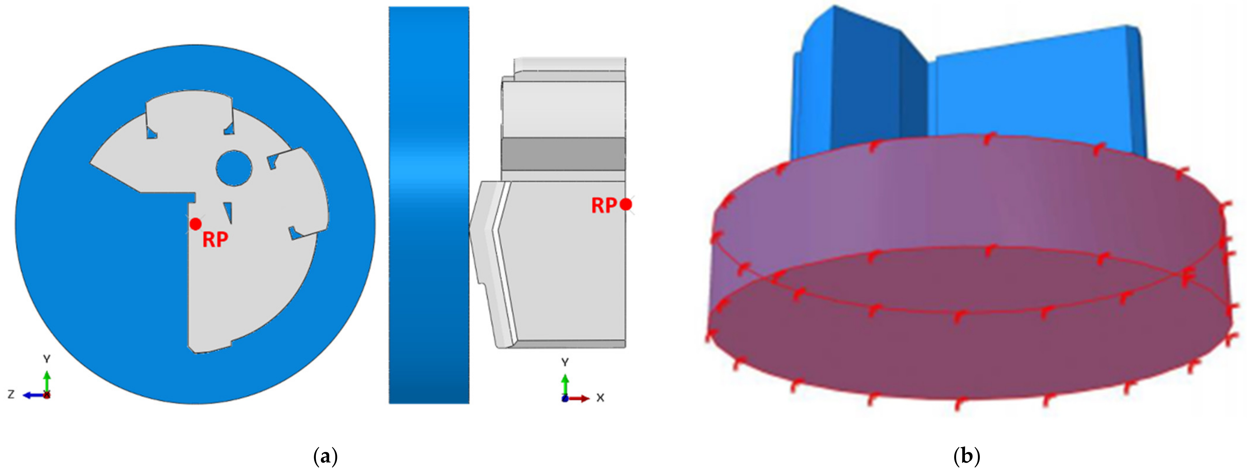
2.2.4. Boundary Conditions
2.2.5. Discretization
2.3. SLD Simulation: Design of Experiments
3. Results
3.1. SLD Simulations
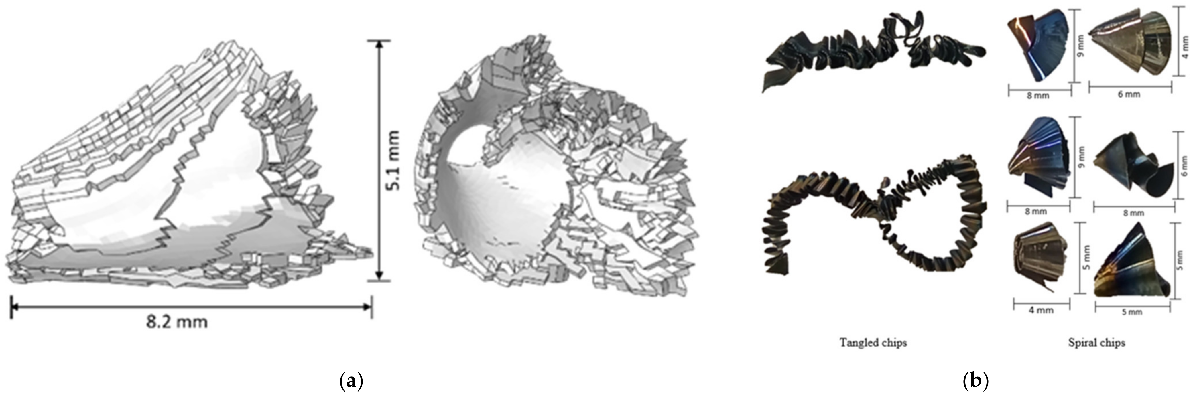
3.1.1. Chip Formation
3.1.2. Temperature Evolution
3.1.3. Feed Force Evolution
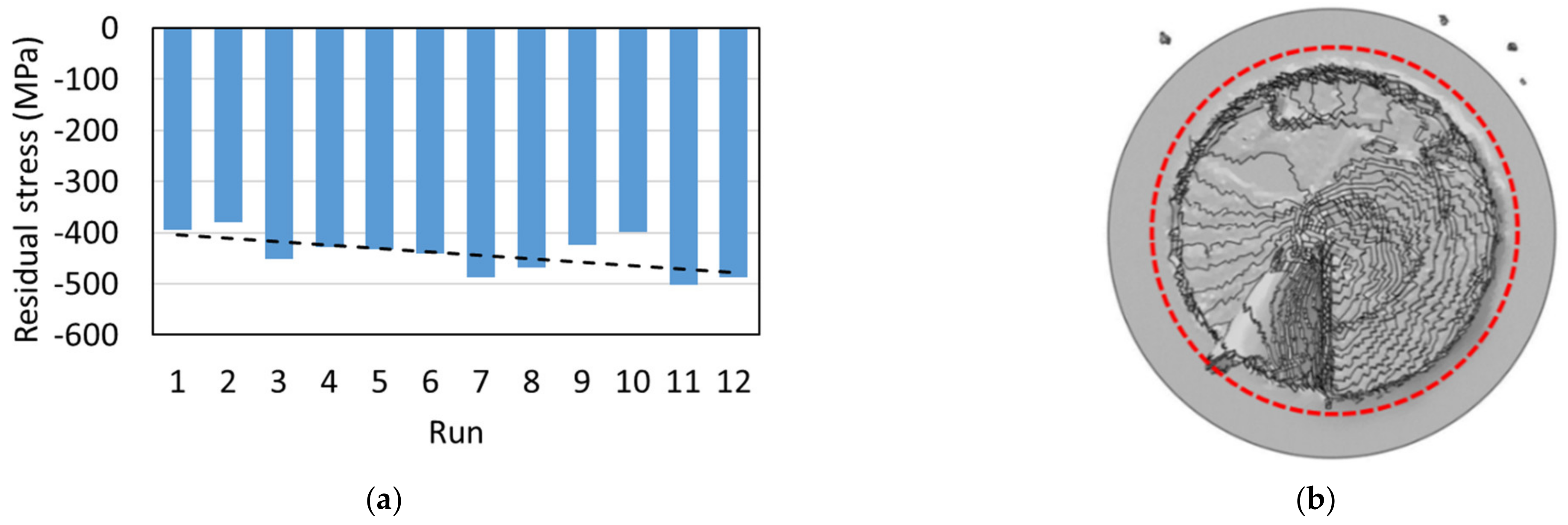
3.1.4. Residual Stress
3.2. SLD Simulation: Design of Experiments
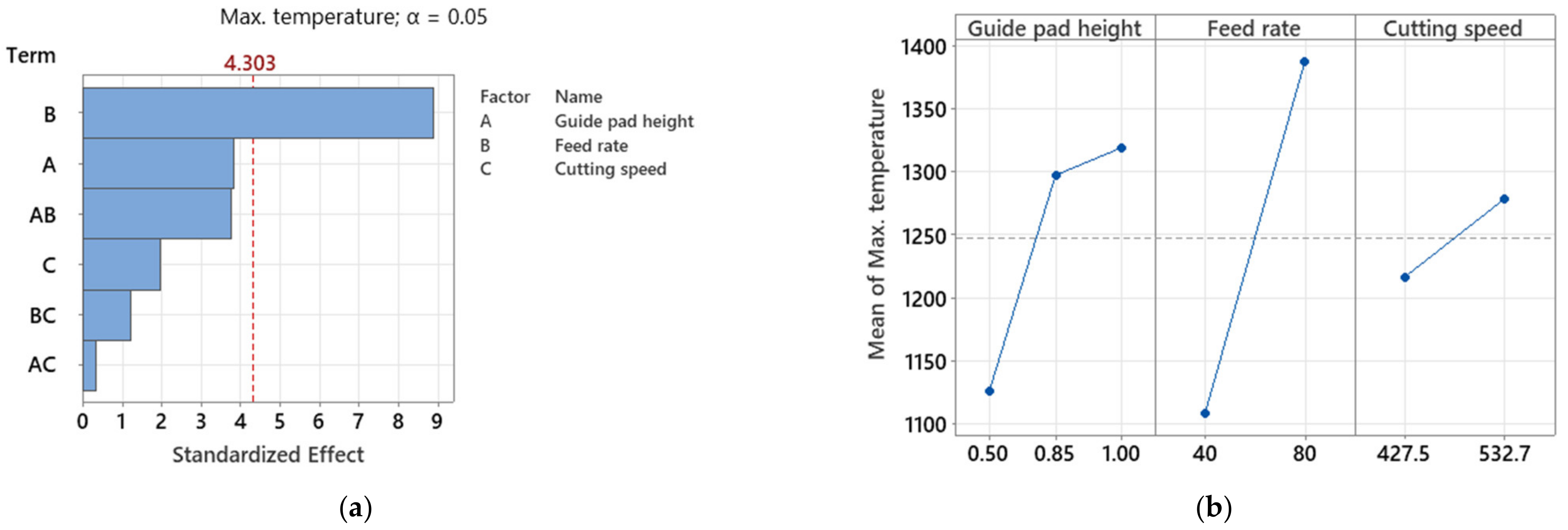
3.2.1. Temperature
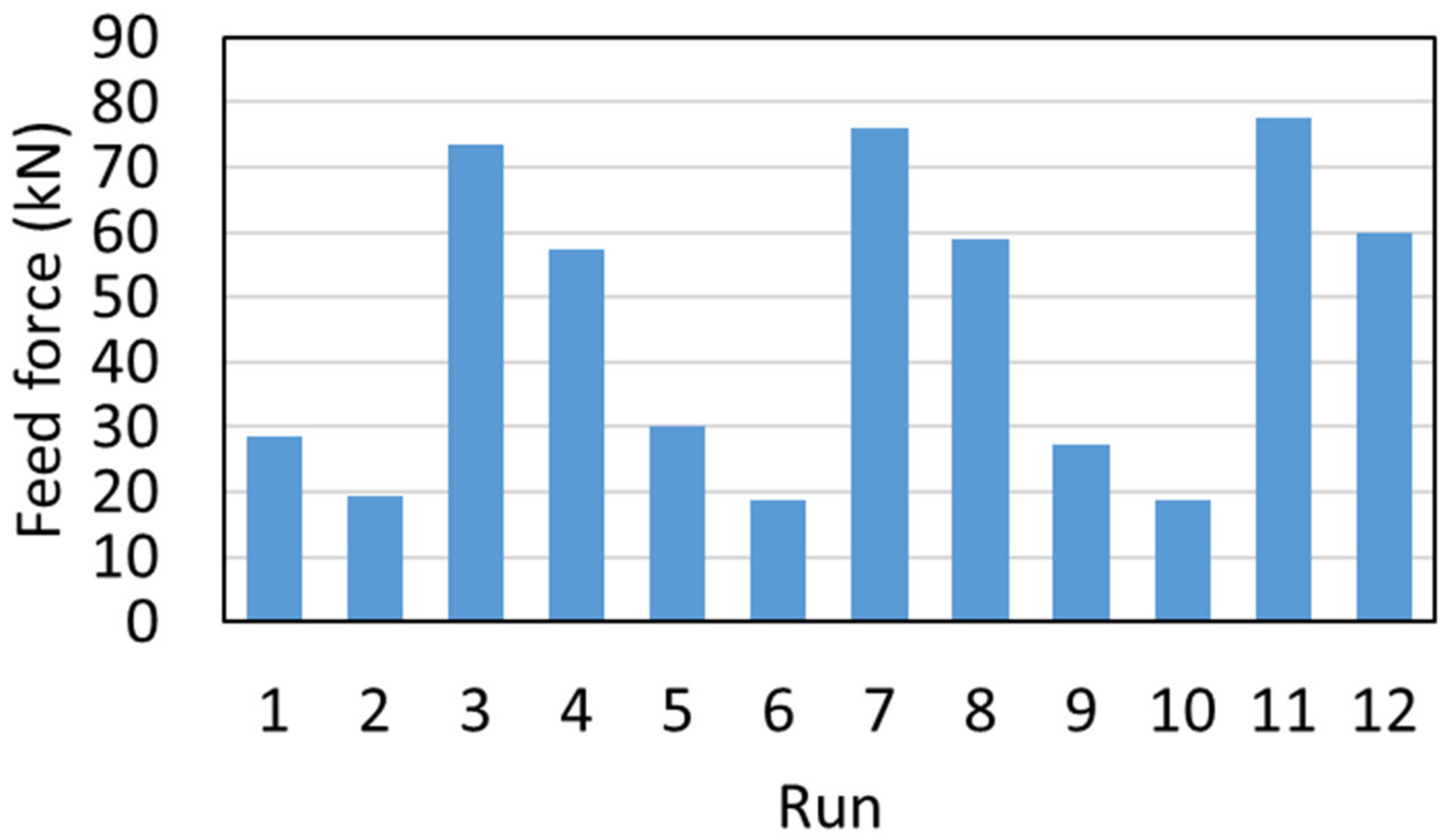
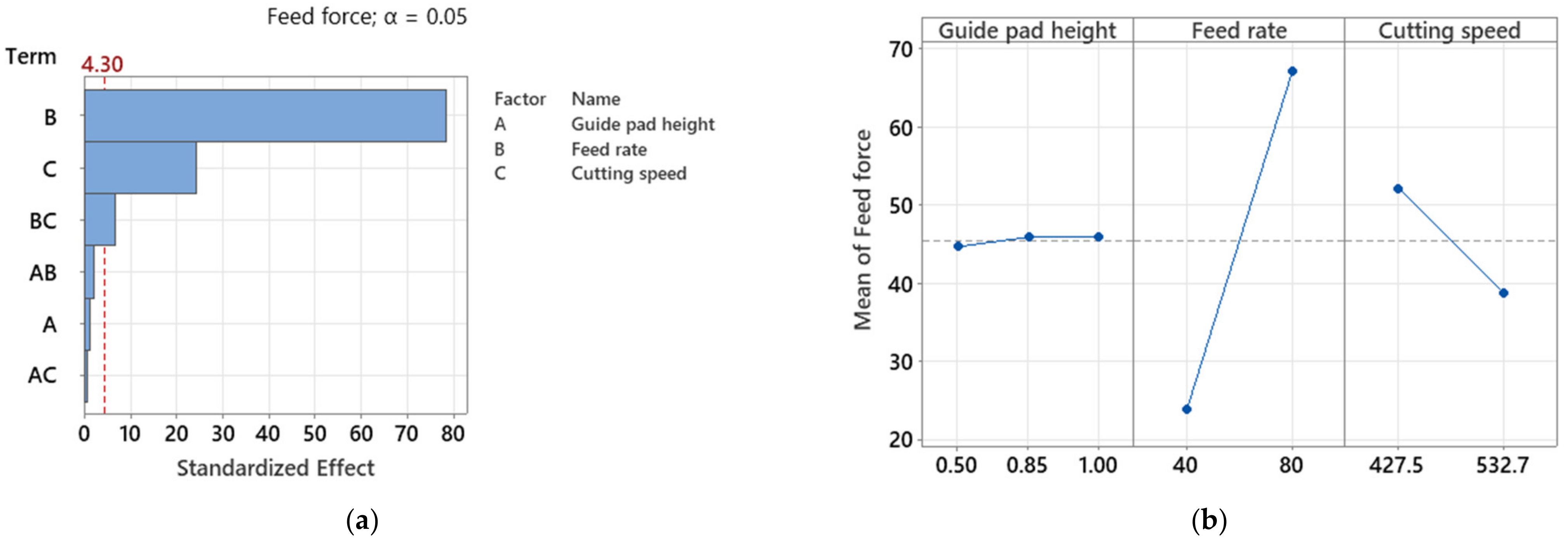
3.2.2. Feed Force
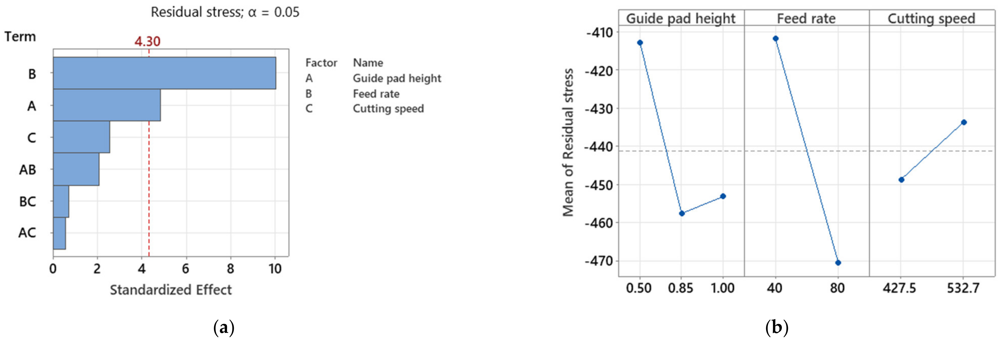
3.2.3. Residual Stress
4. Conclusions
- Although some assumptions and simplifications regarding the drill head and the drilling conditions were made, the chip formation and the temperature evolution were reproduced successfully. Moreover, the feeding force evolution as well as the residual stress were modeled with qualitative agreement.
- A full factorial DoE study was carried out applying three factors with two (feed rate, cutting speed) and three (guide pad height) levels, respectively.
- The extensive DoE study delivered clear effects of the selected factors, such as the feed rate, cutting speed, and guide pad height, on the maximum temperature in the drill head, the feed force, as well as the residual stress in the subsurface.
- The regression model delivers an R2 value of 99.97% for the feed force response, which indicates a high goodness of the results. For the responses of the maximum temperature and residual stress, R2 values of 98.63% and 98.81% were obtained, respectively. These values could be improved by more data or another regression model.
- ANOVA of the maximum temperature shows a significant effect from the feed rate. An increasing feed rate leads to increasing temperatures.
- Significant effects of the feed rate, cutting speed, and the interaction between both on the feed force were obtained by ANOVA. An increasing feed rate and a decreasing cutting speed lead to larger chips, which have to be cut by the driller. Thus, higher forces occur in the process.
- The residual stress is significantly affected by the guide pad height and the feed rate. Increasing factors lead to increasing compressive stresses.
- Regression models for the feed force, maximum temperature, and residual stress were developed, and their corresponding coefficients were successfully determined.
Author Contributions
Funding
Data Availability Statement
Acknowledgments
Conflicts of Interest
Nomenclature
| SLD | Single-lip drill |
| BTA | Boring and Trepanning Association |
| EET | Element elimination technique |
| DoE | Design of experiment |
| CAD | Computer-aided design |
| PTC | Positive temperature coefficient |
| FEM | Finite element method |
| JC | Johnson–Cook |
| ANOVA | Analysis of variance |
| f | Feed per tooth, mm/rev |
| vc | Cutting speed, m/min |
| ρ | Density, kg/m3 |
| ν | Poisson’s ratio |
| E | Young’s modulus, GPa |
| ε | Strain, mm/mm |
| σ | Flow stress, MPa |
| Strain rate, 1/s | |
| λ | Stress triaxiality |
| hGP | Guide pad height, mm |
| δ | Conductivity, W/m K |
| α | Thermal expansion coefficient, µm/m K |
| k | Gap conductance, W/m2 K |
| q | Heat flux per unit area, W/m2 |
| T | Temperature, K |
| Ta | Ambient temperature, K |
| Tm | Melting temperature, K |
References
- Kumari, P. Drilling Machine Market. Available online: alliedmarketresearch.com (accessed on 31 March 2021).
- Biermann, D.; Bleicher, F.; Heisel, U.; Klocke, F.; Möhring, H.C.; Shih, A. Deep hole drilling. CIRP Ann. 2018, 67, 673–694. [Google Scholar] [CrossRef]
- Biermann, D.; Heilmann, M.; Kirschner, M. Analysis of the Influence of Tool Geometry on Surface Integrity in Single-lip Deep Hole Drillingwith Small Diameters. Procedia Eng. 2011, 19, 16–21. [Google Scholar] [CrossRef] [Green Version]
- Agmell, M.; Ahadi, A.; Ståhl, J. A fully coupled thermomechanical two-dimensional simulation model for orthogonal cutting: Formulation and simulation. Proc. Inst. Mech. Eng. B 2011, 225, 1735–1745. [Google Scholar] [CrossRef]
- Agmell, M.; Ahadi, A.; Gutnichenko, O.; Ståhl, J. The influence of tool micro-geometry on stress distribution in turning operations of AISI 4140 by FE analysis. Int. J. Adv. Manuf. Technol. 2017, 89, 9–12. [Google Scholar] [CrossRef] [Green Version]
- Persson, H.; Agmell, M.; Bushlya, V.; Ståhl, J. Experimental and numerical investigation of burr formation in intermittent turning of AISI 4140. Procedia CIRP 2017, 58, 37–42. [Google Scholar] [CrossRef]
- Arrazola, P.J.; Özel, T.; Umbrello, D.; Davies, M.; Jawahir, I.S. Recent advances in modelling of metal machining processes. CIRP Ann. 2013, 62, 695–718. [Google Scholar] [CrossRef]
- Pimenov, D.Y.; Guzeev, V.I. Mathematical model of plowing forces to account for flank wear using FEM modeling for orthogonal cutting scheme. Int. J. Adv. Manuf. Technol. 2017, 89, 3149–3159. [Google Scholar] [CrossRef]
- Pantalé, O.; Bacaria, J.L.; Dalverny, O.; Rakotomalala, R.; Caperaa, S. 2D and 3D numerical models of metal cutting with damage effects. Comput. Methods Appl. Mech. Eng. 2004, 193, 4383–4399. [Google Scholar] [CrossRef] [Green Version]
- Wegert, R.; Guski, V.; Schmauder, S.; Möhring, H.C. Effects on surface and peripheral zone during single lip deep hole drilling. Procedia Cirp 2020, 87, 113–118. [Google Scholar] [CrossRef]
- Aveiro, P. Design of Experiments in Production Engineering; Davim, J.P., Ed.; Springer International Publishing: Basel, Switzerland, 2016. [Google Scholar]
- Kyratsis, P.; Bilalis, N.; Antoniadis, A. CAD-based simulations and design of experiments for determining thrust force in drilling operations. Comput. Aided Des. 2011, 43, 1879–1890. [Google Scholar] [CrossRef]
- Chatterjee, S.; Mahapatra, S.S.; Abhishek, K. Simulation and optimization of machining parameters in drilling of titanium alloys. Simul. Model. Pr. Theory 2016, 62, 31–48. [Google Scholar] [CrossRef]
- Wegert, R.; Guski, V.; Möhring, H.C.; Schmauder, S. Determination of thermo-mechanical quantities with a sensor-integrated tool for single lip deep hole drilling. Procedia Manuf. 2020, 52, 73–78. [Google Scholar] [CrossRef]
- Wegert, R.; Guski, V.; Möhring, H.C.; Schmauder, S. Temperature monitoring in the subsurface during single lip deep hole drilling: Measuring of the thermo-mechanical load at different cutting parameters, including wear and simulative validation. tm-Tech. Mess. 2020, 87, 757–767. [Google Scholar] [CrossRef]
- Brnic, J.; Turkalj, G.; Canadija, M.; Lanc, D.; Brcic, M. Study of the effects of high temperatures on the engineering properties of steel 42CrMo4. High Temp. Mater. Process. 2015, 34, 27–34. [Google Scholar] [CrossRef]
- Storchak, M.; Rupp, P.; Möhring, H.C.; Stehle, T. Determination of Johnson–Cook constitutive parameters for cutting simulations. Metals 2019, 9, 473. [Google Scholar] [CrossRef] [Green Version]
- Johnson, G.R.; Cook, W.H. Fracture characteristics of three metals subjected to various strains, strain rates, temperatures and pressures. Eng. Fract. Mech. 1985, 21, 31–48. [Google Scholar] [CrossRef]
- ABAQUS. Version 2018, ABAQUS Documentation, Dessault Systems Simulia Corp; ABAQUS: Providence, RI, USA, 2018. [Google Scholar]
- Barge, M.; Hamdi, H.; Rech, J.; Bergheau, J. Numerical modelling of orthogonal cutting: Influence of numerical parameters. J. Mater. Process. Technol. 2005, 164, 1148–1153. [Google Scholar] [CrossRef]
- Mabrouki, T.; Rigal, J. A contribution to a qualitative understanding of thermo-mechanical effects during chip formation in hard turning. J. Mater. Process. Technol. 2006, 176, 214–221. [Google Scholar] [CrossRef]
- Schulze, V.; Michna, J.; Zanger, F.; Faltin, C.; Maas, U.; Schneider, J. Influence of cutting parameters, tool coatings and friction on the process heat in cutting processes and phase transformations in workpiece surface layers. Htm J. Heat Treat. Mater. 2013, 68, 22–31. [Google Scholar] [CrossRef]
- Fluhrer, J. DEFORM 3D Version 6.1 User´s Manual; Scientific Forming Technologies Corporation-SFTC: Columbus, OH, USA, 2007. [Google Scholar]
- Koric, S.; Hibbeler, L.; Thomas, B. Explicit coupled thermo-mechanical finite element model of steel solidification. Int. J. Numer. Methods Eng. 2009, 78, 1–31. [Google Scholar] [CrossRef] [Green Version]
- Prior, M. Applications of implicit and explicit finite element techniques to metal forming. J. Mater. Process. Technol. 1994, 45, 649–656. [Google Scholar] [CrossRef]
- Rajput, R. A Textbook of Manufacturing Technology: Manufacturing Processes; Laxmi Publications: New Delhi, India, 2007. [Google Scholar]
- ASTM. E837: Standard Test Method for Determining Residual Stresses by the Hole-Drilling Strain-Gage Method; ASTM International: West Conshohocken, PA, USA, 2013. [Google Scholar]


| Young’s Modulus (GPa) | Poisson’s Ratio (-) | Temperature (K) |
|---|---|---|
| 217 | 0.3 | 173 |
| 213 | 0.3 | 273 |
| 212 | 0.3 | 293 |
| 207 | 0.3 | 373 |
| 199 | 0.3 | 473 |
| 192 | 0.3 | 573 |
| 184 | 0.3 | 673 |
| 175 | 0.3 | 773 |
| 164 | 0.3 | 873 |
| 69 | 0.3 | 1773 |
| A (MPa) | B (MPa) | C (-) | n (-) | m (-) | Tm (K) | Ta (K) |
|---|---|---|---|---|---|---|
| 595 | 580 | 0.023 | 0.133 | 1.03 | 1793 | 300 |
| d1 | d2 | d3 | d4 | d5 | (K) | (K) | (1/s) |
|---|---|---|---|---|---|---|---|
| 0.1 | 0.04 | −0.02 | 1 | 0.12 | 1793 | 300 | 1 |
| Temperature (K) | Thermal Expansion (µm/m K) | Conductivity (W/m K) | Specific Heat (J/kg K) |
|---|---|---|---|
| 173 | 10.8 | - | 291.24 |
| 273 | 11.7 | - | 354.04 |
| 293 | 11.9 | 41.7 | 361.89 |
| 373 | 12.5 | 43.4 | 389.36 |
| 473 | 13.0 | 43.2 | 418.41 |
| 573 | 13.6 | 41.4 | 445.88 |
| 673 | 14.1 | 39.1 | 479.64 |
| 773 | 14.5 | 36.7 | 531.45 |
| 873 | 14.9 | 34.1 | 610.73 |
| 1773 | 14.9 | 34.1 | 610.73 |
| 1923 | - | 34.1 | 610.73 |
| Property | Unit | Value |
|---|---|---|
| Density, ρ | kg/m3 | 15,700 |
| Young’s modulus, E | GPa | 524 |
| Poisson’s ratio, ν | - | 0.23 |
| Thermal expansion, α | µm/m K | 6.3 |
| Conductivity, δ | W/m K | 82.2404 |
| Specific heat, Cp | J/kg K | 579.45 |
| Run Order | Guide Pad Height (mm) | Feed Rate (mm/s) | Cutting Speed (m/min) |
|---|---|---|---|
| 1 | 0.5 | 40 | 427.5 |
| 2 | 0.5 | 40 | 532.7 |
| 3 | 0.5 | 80 | 427.5 |
| 4 | 0.5 | 80 | 532.7 |
| 5 | 0.85 | 40 | 427.5 |
| 6 | 0.85 | 40 | 532.7 |
| 7 | 0.85 | 80 | 427.5 |
| 8 | 0.85 | 80 | 532.7 |
| 9 | 1.00 | 40 | 427.5 |
| 10 | 1.00 | 40 | 532.7 |
| 11 | 1.00 | 80 | 427.5 |
| 12 | 1.00 | 80 | 532.7 |
| Term | Coefficient | SE Coefficient | T-Value | p-Value |
|---|---|---|---|---|
| Constant | 1247.7 | 15.8 | 79.05 | 0.0 |
| Guide pad height (A) | ||||
| 0.5 | −121.7 | 22.3 | −5.45 | 0.032 |
| 0.85 | 49.8 | 22.3 | 2.23 | 0.155 |
| Feed rate (B) | ||||
| 40 | −140.0 | 15.8 | −8.87 | 0.012 |
| Cutting speed (C) | ||||
| 427.5 | −31.2 | 15.8 | −1.97 | 0.187 |
| Guide pad height, feed rate (AB) | ||||
| 0.50, 40 | 121.0 | 22.3 | 5.42 | 0.032 |
| 0.85, 40 | −59.0 | 22.3 | −2.64 | 0.118 |
| Guide pad height, Cutting speed (AC) | ||||
| 0.50, 427.5 | −17.3 | 22.3 | −0.78 | 0.519 |
| 0.85, 427.5 | 12.7 | 22.3 | 0.57 | 0.628 |
| Feed rate, cutting speed (BC) | ||||
| 40, 427.5 | −19.5 | 15.8 | −1.24 | 0.342 |
| Term | Coefficient | SE Coefficient | T-Value | p-Value |
|---|---|---|---|---|
| Constant | 45.446 | 0.277 | 164.19 | 0.0 |
| Guide pad height (A) | ||||
| 0.5 | −0.813 | 0.391 | −2.08 | 0.172 |
| 0.85 | 0.404 | 0.391 | 1.03 | 0.410 |
| Feed rate (B) | ||||
| 40 | −21.672 | 0.277 | −78.30 | 0.0 |
| Cutting speed (C) | ||||
| 427.5 | 6.683 | 0.277 | 24.14 | 0.002 |
| Guide pad height, feed rate (AB) | ||||
| 0.50, 40 | 0.970 | 0.391 | 2.48 | 0.131 |
| 0.85, 40 | 0.207 | 0.391 | 0.53 | 0.649 |
| Guide pad height, cutting speed (AC) | ||||
| 0.50, 427.5 | −0.385 | 0.391 | −0.98 | 0.429 |
| 0.85, 427.5 | 0.427 | 0.391 | 1.09 | 0.389 |
| Feed rate, cutting speed (BC) | ||||
| 40, 427.5 | −1.862 | 0.277 | −6.73 | 0.021 |
| Term | Coefficient | SE Coefficient | T-Value | p-Value |
|---|---|---|---|---|
| Constant | 441.15 | 2.94 | −150.24 | 0.0 |
| Guide pad height (A) | ||||
| 0.50 | 28.46 | 4.15 | 6.85 | 0.021 |
| 0.85 | −16.45 | 4.15 | −3.96 | 0.058 |
| Feed rate (B) | ||||
| 40 | 29.40 | 2.94 | 10.01 | 0.010 |
| Cutting speed (C) | ||||
| 427.5 | −7.51 | 2.94 | −2.56 | 0.125 |
| Guide pad height, feed rate (AB) | ||||
| 0.50, 40 | −3.21 | 4.15 | −0.77 | 0.520 |
| 0.85, 40 | −9.20 | 4.15 | −2.22 | 0.157 |
| Guide pad height, cutting speed (AC) | ||||
| 0.50, 427.5 | −2.25 | 4.15 | −0.54 | 0.642 |
| 0.85, 427.5 | 4.59 | 4.15 | 1.10 | 0.384 |
| Feed rate, cutting speed (BC) | ||||
| 40, 427.5 | 2.10 | 2.94 | 0.72 | 0.549 |
Publisher’s Note: MDPI stays neutral with regard to jurisdictional claims in published maps and institutional affiliations. |
© 2021 by the authors. Licensee MDPI, Basel, Switzerland. This article is an open access article distributed under the terms and conditions of the Creative Commons Attribution (CC BY) license (https://creativecommons.org/licenses/by/4.0/).
Share and Cite
Fandiño, D.; Guski, V.; Wegert, R.; Möhring, H.-C.; Schmauder, S. Simulation Study on Single-Lip Deep Hole Drilling Using Design of Experiments. J. Manuf. Mater. Process. 2021, 5, 44. https://0-doi-org.brum.beds.ac.uk/10.3390/jmmp5020044
Fandiño D, Guski V, Wegert R, Möhring H-C, Schmauder S. Simulation Study on Single-Lip Deep Hole Drilling Using Design of Experiments. Journal of Manufacturing and Materials Processing. 2021; 5(2):44. https://0-doi-org.brum.beds.ac.uk/10.3390/jmmp5020044
Chicago/Turabian StyleFandiño, Daniel, Vinzenz Guski, Robert Wegert, Hans-Christian Möhring, and Siegfried Schmauder. 2021. "Simulation Study on Single-Lip Deep Hole Drilling Using Design of Experiments" Journal of Manufacturing and Materials Processing 5, no. 2: 44. https://0-doi-org.brum.beds.ac.uk/10.3390/jmmp5020044