Article

Prediction of Machining Condition Using Time Series Imaging and Deep Learning in Slot Milling of Titanium Alloy

by
Faramarz Hojati
*,
Bahman Azarhoushang
,
Amir Daneshi
and
Rostam Hajyaghaee Khiabani
Institute of Precision Machining (KSF), Furtwangen University, 78532 Tuttlingen, Germany
*
Author to whom correspondence should be addressed.
J. Manuf. Mater. Process. 2022, 6(6), 145; https://0-doi-org.brum.beds.ac.uk/10.3390/jmmp6060145
Submission received: 17 October 2022 / Revised: 10 November 2022 / Accepted: 13 November 2022 / Published: 16 November 2022

Abstract

:
Low surface quality, undesired geometrical and dimensional tolerances, and product damage due to tool wear and tool breakage lead to a dramatic increase in production cost. In this regard, monitoring tool conditions and the machining process are crucial to prevent unwanted events during the process and guarantee cost-effective and high-quality production. This study aims to predict critical machining conditions concerning surface roughness and tool breakage in slot milling of titanium alloy. Using the Siemens SINUMERIK Edge Box integrated into a CNC machine tool, signals were recorded from main spindle and different axes. Instead of extraction of features from signals, the Gramian angular field (GAF) was used to encode the whole signal into an image with no loss of information. Afterwards, the images obtained from different machining conditions were used for training a convolutional neural network (CNN) as a suitable and frequently applied deep learning method for images. The combination of GAF and trained CNN model indicates good performance in predicting critical machining conditions, particularly in the case of an imbalanced dataset. The trained classification CNN model resulted in recall, precision, and accuracy with 75%, 88%, and 94% values, respectively, for the prediction of workpiece surface quality and tool breakage.

1. Introduction

Cutting tool breakage or severe tool wear cause low product quality or even scrap production, damage to machine components or unexpected production downtime. For this reason, tool breakage should be prohibited, and a tool should be changed before being subjected to severe wear. However, earlier tool change increases the tool cost and tool changing cost (due to production down-time during the tool change), which is a remarkable share of the total production cost. With tool wear prediction or detection, the cutting tool can be changed at an appropriate time interval to avoid damage or quality failures [1].
In recent years, extensive research works have been conducted to monitor the condition of cutting tools during the process for optimizing tool lifespan [2], early detection of tool wear, and prevention of tool breakage [3]. Direct monitoring of the cutting tool, which measures the tool geometry using vision or optical apparatus, requires expensive equipment and cannot be applied in real-time, among other issues, due to the presence of coolant and the contact between the tool and material [4]. Therefore, the focus of research activities was mainly on indirect approaches of tool and machining condition monitoring, which benefit from the fact that a variation in cutting tool condition changes certain variables such as cutting forces, vibration, and surface finish. In these methods, the machine data (such as the current, power, and so on) from the machine elements (such as spindle or axis motors) [5,6,7] or signals from the sensors integrated into the machine tool (such as piezosensor, accelerometer, strain gauge, thermocouple, acoustic emission sensor, and so on) [8,9,10,11,12,13,14,15,16] are analyzed to recognize the possible correlations with the cutting tool and machining condition. Olma et al. [17] presented an efficient method for monitoring high-speed broaching for Inconel 718 using process vibrations recorded by accelerometers. In this regard, analyzing time and frequency domain signals, considering tooth pass frequency and harmonics, were carried out. The results indicate a useful method for using in daily life production. However, due to the complex and unpredictable progress of tool wear during the machining process, introducing signal features or algorithms showing the best correlation with the wear states of the cutting tool is difficult. In addition, the process parameters and cutting conditions can significantly influence sensor signals and may lead to remarkable noises in the measurement. For these reasons, multiple sensors are integrated into the machine tool to acquire data with a high signal-to-noise ratio in practice. In this regard, Nasir et al. [18] conducted an investigation regarding tool condition monitoring using power, sound, vibration and acoustic emission (AE) signals. The authors discussed a trade-off between accuracies of classifiers and the tolerance for sensor redundancy playing an important role in the optimal combination of sensors. Ou et al. [19] applied sound pressure signals, acceleration signals, and spindle motor current signals and confused them into images as monitoring samples. Kuntoğlu et al. [20] used five sensors of acoustic emission, current, temperature, force and vibration to monitor tool condition with respect to flank wear. They concluded the acoustic emission and temperature signals were found effective for detecting tool flank wear. Zhang et al. [8], in addition to capturing the machine power signal, employed a 3-axis accelerometer and two piezosensors to monitor vibration and cutting forces, respectively. They observed that total power and acceleration signals could effectively highlight the processing condition. A failure in cutting by identifying the abnormal peak values of recorded signals was detected. Finally, it was demonstrated that the trend of the total power signal is in accordance with that introduced by the Taylor model [21] for predicting tool life. This confirmed a feasible tool wear monitoring. Hesser and Markert [9] applied an acceleration sensor to detect tool wear during milling. The concept of their work was based on the fact that the cutting force and, simultaneously, process vibrations increase once the tool wear initiates. The higher cutting force and process vibrations, in turn, result in a higher magnitude of the acceleration signal. After training an artificial neural network (ANN) model using accelerometer signals, the tool condition could be classified into two groups (new tool and worn tool). In addition to the acceleration sensor, acoustic emission (AE) and force sensors have been utilized for tool wear detection in various studies. Wang et al. [22] evaluated tool wear using clustering energy of AE signals induced by minimum quantity lubrication (MQL), material fracture and workpiece plastic deformation. A linear relation between flank wear and the total energy of AE signals induced by workpiece material fracture and plastic deformation was found. Tahir et al. [23] measured the cutting forces in milling by piezoelectric sensors and analyzed the cutting force signals in time and frequency domains. The results indicate that the main cutting force correlates with the evolution of the tool flank wear. An increase in the amplitude of the main cutting force was observed with increasing flank wear. Another research work, conducted by Nouri et al. [4], introduced a method based on cutting force coefficients for tool condition monitoring. After starting chipping at the cutting tool, an increase in force coefficients with considerable variability in their magnitude was observed. A dramatic change in the tool geometry was highlighted by a fluctuation in cutting force coefficients and was considered as a transition from gradual wear to a failure region. Accordingly, it was concluded that the tangential and radial cutting force coefficients also correlate with tool flank wear and could be used to monitor the tool wear. Zhou et al. [24] applied sound singularity analysis for tool condition monitoring in the milling process. A significant qualitative correlation between sound waveform singularities and tool wear progress was observed. Using a support vector machine (SVM) as a classification model, a prediction accuracy of 85% was obtained. Machine vision-based tool condition monitoring has also gained high popularity in recent years. In this method, the image matrices of the final surfaces are analyzed through different algorithms (such as classification or regression algorithms) to extract decisive features for tool monitoring [25]. Dutta et al. [26] analyzed the machined surfaces and extracted the features correlating well with the tool wear progress. Four features were extracted from the machined surface images using gray level co-occurrence matrix-based (GLCM) and discrete wavelet transform-based (DWT) texture analyses techniques. It was demonstrated that all extracted features increase with the average flank wear of the tool. Lin et al. [27] applied accelerator vibration signals combined with deep learning predictive models for predicting surface roughness. They have used three models: the fast Fourier transform–deep neural network (FFT-DNN), fast Fourier transform–long short-term memory network (FFT-LSTM), and one-dimensional convolutional neural network (1-D CNN) to explore training and prediction performances. Based on the results, the use of prediction of the surface roughness via vibration signals using FFT-LSTM or 1-D CNN is recommended to develop an intelligent system. Bhandari et al. [28] conducted a non-contact surface roughness evaluation using a convolutional neural network (CNN). The machined surface images were used to develop CNN models for surface roughness prediction in four classes of fine, smooth, rough, and coarse. Based on the developed model, the training and test accuracy of 96.30% and 92.91% were reported, respectively. Rifai et al. [29] applied the CNN model for prediction of surface roughness. The prediction was based on the ridge–valley pattern of the cutter marks. The proposed model was evaluated for outside diameter turning, slot milling, and side milling, at various cutting conditions.
Apart from the proposed methods, the term of digital twining has been highlighted for the manufacturing process by Magalhães [30]. According to Liu et al. [31], digital twining provides high-fidelity virtual entities of physical entities for observing, analyzing, and controlling the machining process in real-time. In [32], the multi-dimensional modeling approach for machining processes, by introducing digital twin (DT) technology was presented. As reported, application of digital twining increased the material removal rate and reduced deformation in key components of diesel engines.
The tool and process condition monitoring methods generally need to extract the features of the measured signal (after recording the signals) manually to use them for model training. In this regard, the application of the utilized algorithm in the extraction of features varies from signal to signal, and the feature extraction requires a well-experienced person. Moreover, some information on the signal through the feature extraction would be lost. To solve this issue, imaging the signals using different approaches, such as Gramian angular field [33] rather than feature extraction, can be helpful. As an example, Arellano et al. [34] applied GAF for tool wear classification. The recorded cutting force signals were encoded to several images that have been used for training a convolutional neural network (CNN) classification model. A percentage of accuracy over 80% was reported for different groups, corresponding to different states of tool wear (break-in, steady-state, and failure).
A need for analyzing the signal for process monitoring is growing with a new generation of machine tools capable of recording different types of data. The Siemens SINUMERIK EDGE (SE) Box, that can be integrated into the machine tool, records the signals from different axes and main spindles and fuses all measured data into a JSON file. The signals for recording are selected in the MindSphere Capture4Analysis application, which is connected to the SINUMERIK Edge Box. The current study aims to predict the machining condition using different types of signals recorded by the SINUMERIK Edge Box integrated into the five axes CNC machine tool (Haas-Multigrind® CA, Trossingen, Germany). The experimental tests were conducted in milling a titanium alloy (Ti6Al4V) as a difficult-to-cut material. Severe tool wear and even tool breakage due to a built-up edge (BUE), particularly at high-speed machining of the titanium alloy, followed by low workpiece surface quality, was detected. After measuring signals, GAF, as one of the time series imaging methods, was applied for encoding the signals into images. Further, images were used for training the CNN classification model to predict the critical machining condition. Eventually, the combination of the GAF and CNN model was evaluated.

2. Materials & Methods

In this investigation, Ti6Al4V was selected as the workpiece material. Slot milling was used as a milling strategy. The milling tests were carried out with different process parameters. In all tests, the axial depth of cut ap was kept constant and equal to 1 mm, and the radial depth of cut ae was 3 mm. The feed per tooth, fz, and cutting speed vc were considered as varying parameters. A total of 161 tests (each test including 6 slot milling passes) were carried out with different combinations of varying process parameters. The tests were conducted with and without coolant lubricant. In the presence of cooling, no tool wear and tool breakage were observed. Therefore, several tests were also carried out without coolant lubricant (dry cutting) at the higher range of feeds and cutting speeds to increase the tool wear rate and reduce the required experimental time. Table 1 provides the range of milling parameters.
Figure 1 indicates the integration of the whole data acquisition system into the utilized milling machine. A five axes CNC machine tool (Haas-Multigrind® CA, Trossingen, Germany) with a Siemens Sinumerik controller used in this study. For the data acquisition, the machine tool is equipped with a so-called Siemens SINUMERIK EDGE (SE) Box. Siemens CNC controls supply data, and SE, making it possible to record data and states of the control in a resolution of 1 ms (1kHz) parallel to the process. The SE box is, in principle, an industrial computer and has the corresponding resources to store the data. The MindSphere Capture4Analysis application enables the selection of the signals to be recorded and the trigger time from which a signal is to be recorded. According to a defined system, the data is written to a JSON file on the hard disk of the SE box with the execution of the NC program. Further, the JSON File for each test is processed through a written ETL program (extract–transform–load) to obtain the tabular data in CSV format. The CSV data and post-process information from the measurement system collected in tabular data are imported directly into an artificial intelligence (AI) Model. Moreover, the CSV data can also be visualized using an external computer for the machine tool user.
The concept of the utilized AI Model is shown in Figure 1. Instead of using the signals features such as mean, peak and standard deviation, each signal was converted into an image by Gramian angular field (GAF), which contains all the features as well as the relationships between different points of the signal. In the next step, the images were used as input parameters for training the CNN model. Finally, the model can predict the quality of the process concerning the critical machining condition in terms of machined surface roughness and tool breakage with respect to new images obtained from new signals (even with different process parameters). In this section, the AI model is explained in detail.
Figure 2a illustrates the experimental setup. The milling tool moved from the right side to the left side of the workpiece (according to the milling direction shown in Figure 2a), and for the creation of slots with a depth of 6 mm, six slot milling passes each with axial depth of cut, ap, of 1 mm were conducted. The signals from different axes of the machine tool were recorded through the SE Box system and saved as a JSON file. Figure 2b illustrates the different axes in the HAAS machine tool. The types of signals that the Edge Box for the main spindle and each axis can record are categorized into current, load, torque and power, and are described in section results and discussions. At each milling pass, the Edge Box started to automatically record the signals slightly prior to the slot milling process and the recording was automatically stopped after the cutting process.
Figure 3a shows the geometrical properties of the utilized tools. The milling tools were coated with AlTiN. D1, D2, L1, L2, EF and Z are cutting tool and shank diameter, total length, cutting edge length, corner chamfer and the number of teeth, respectively. Figure 3b–d also demonstrated three cutting edges of a new tool.

3. Signal Selection

As explained in the previous section, after recording the signals through the Edge Box, the data from JSON files for each experiment were extracted. Figure 4 illustrates different types of signals in terms of current, load, power and torque recorded by Edge Box in the spindle and various axes of the machine tool for the first pass of slot milling at vc = 50 m/min and fz = 30 µm/tooth. Signals showing a change when the milling tool came into contact with the workpiece, were used for further analysis. For the current signal, the difference between machining time and non-machining time could be observed from axes of A, C, SP1, Y, and Z. In the case of load signal, the axes of A, C, Y, and Z differentiate between contact and non-contact time. Regarding the power signal, the only axis that indicated such a difference is SP1, although it is not considerable in this figure. The axes of A, C, Y and Z highlight the contact time between tool and workpiece for the torque signal.
In the next step, the sensitivity of each signal against changing machining conditions was investigated to find the signals with informative data. In this regard, after observing the potential signals in different experiments, it was concluded that the signals in the z-axis for current, load and torque are the best candidates for model training. In detail, the signals in other axes showed no remarkable change before tool breakage, while the mentioned types of signals in the z-axis considerably altered.
Figure 5 illustrates an example of these signals before the tool breakage. After the second pass, a considerable fluctuation in all types of the signal can clearly be observed. This can be associated with considerable built-up edge (BUE) at the dry milling of titanium alloys, that was eventually followed by tool breakage. Figure 6 shows a considerable BUE at vc = 80 m/min and fz = 20.6 µm/tooth that led to cutting edge and tool breakage.
According to Figure 5, the response of three different types of signals (current, load and torque) are similar and using all of them for training the model is not required. Therefore, the load signal was used for further analysis.

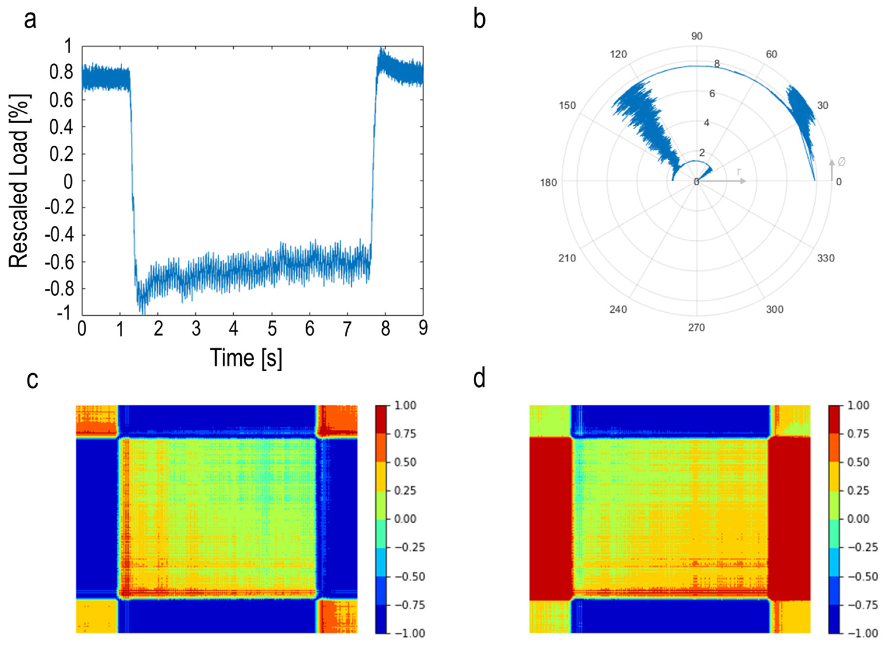
4. Gramian Angular Field (GAF)

The GAF algorithm is used for encoding the time series signal into an image, resulting in transferring the signal to a polar coordinate space. First, the signal points X = x 1 , x 2 , x 3 , , x n are normalized so that all values fall in the range of [−1,1] (See Figure 7a).
x ˜ i = x i max X + x i min X max X min X
The rescaled signal X ˜ = x ˜ 1 , x ˜ 2 , x ˜ 3 , , x ˜ n is transformed in the polar system using the following equations:
= arccos x ˜ i , 1 x ˜ i 1   ,   x ˜ i X ˜ r = t i N  
where Ø and r are angular positions and the radius for determining the position of each point in the polar space. The ti is the corresponding time of the signal points. Moreover, N is a constant and is considered as a regularization factor for polar space span. This value was set to 1 in this study. Figure 7b represents the rescaled signal in the polar coordinate.
Next, the GAF algorithm is applied for encoding the polar coordinate of the normalized time series into an image to produce a temporal correlation between different time series points. Using a Gramian angular summation field (GASF), the trigonometric sum is applied to each couple of angular positions of each time series point and the rest of the signal points for generating each row of the GASF matrices. Therefore, the temporal correlation between each point of the signal and the rest of the signal is calculated at each row, as below:
GASF = cos 1 + 1 cos 1 + n cos 2 + 1 cos 2 + n cos n + 1 cos n + n
For the construction of Gramian angular difference field (GADF) matrices, the couple of angular positions of each time series point and the rest points are subjected to the trigonometric difference, as described in the following equation:
GADF = sin 1 1 sin 1 n sin 2 1 sin 2 n sin n 1 sin n n
Two matrices of GASF and GADF are illustrated in Figure 7c,d. It is possible to apply the GASF or GADF methods for further analysis. In this study, GASF images have been used. In the produced GASF image, some regions are related to the non-machining area, which are not informative for use in the model training. Therefore, these areas are removed to reduce the computational time and prevent any inaccuracy in further analysis (See Figure 8).
Figure 9 provides the signals and corresponding GASF images for a series of five pass-milling prior to the tool breakage. At the first two passes, no remarkable change in the image (and correspondingly the row signals) can be observed, while afterwards, a dramatic change in images (alteration in the colors and pattern of images) associated with the signal fluctuation can clearly be seen, followed by tool breakage in the fifth pass.

5. Clustering Images

Before training the CNN model, the images were clustered into two main groups (A and B). Group A contains all images from experiments where no tool breakage occurred. The build-up edge resulted in an unstable condition followed by tool breakage. Before tool breakage, a remarkable fluctuation was observed in the signals (and correspondingly changing the color and pattern of images), which can be considered as an alarm for tool breakage and belongs to group B. In some experiments, such a fluctuation in the signals was also observed, but no tool breakage occurred. Instead, the surface quality deteriorated dramatically, as shown in Figure 10a,b, which indicates the milled surface has considerably better quality and, therefore, its corresponding GASF image is associated with group A.
Figure 11 also shows the quantitative analysis of the generated surfaces from different milling series with respect to the roughness values (Ra and Rz). Accordingly, the images change significantly at higher values of Ra and Rz (red ellipse). Therefore, the GASF images from these tests were also included in group B.
Eventually, group B contains all images belonging to the experimental tests where tool breakage occurred, or the surface quality deteriorated dramatically. Therefore, these two phenomena should be avoided in the machining process and are included in group B as critical conditions. Meanwhile, group A includes images of the tests where no tool breakage occurred, and acceptable surface quality was induced. A total of 858 GASF images were produced in this study. Based on the assumption regarding the clustering of images in two groups, 726 and 132 images corresponded to group A and group B, respectively.

6. Convolutional Neural Network (CNN)

A convolutional neural network (CNN), a commonly applied method for machine learning of images, was used as a classification model in this study. Figure 12 illustrates the architecture of the developed CNN model. Two main components in this model are the convolution layer and the pooling layer. In the convolution layer, multiple filters are applied to the imported image. Each filter scans the entire image, and at each position, the similarity of the filter is compared with that area of the image. The output of the convolution layer results in several images that are smaller than the original image. The number of images corresponds to the number of applied filters. In the next step, the pooling layer is applied to reduce the size of the images and, correspondingly, the number of parameters to be learned as well as the number of computations performed in the network. Moreover, the pooling layer extracts the most important features of the image. Therefore, the images are imported from the convolution layer to the pooling layer, which results in a dimension reduction while preserving the important features of the images. Finally, the images are flattened and imported into the neural network for training.
After creating the images using the GASF method, they are resized to 224 × 224 for importing into the CNN model. In this study, two convolution layers were determined. The number and size of filters for each convolution layer accounted for 128 and 3 × 3, respectively. After each convolution layer, a pooling layer is placed with a pool size of 2 × 2. Therefore, the imported images (with the size of 224 × 224) after the first convolution layer are reduced to 222 × 222. Further, 128 images obtained from the first convolution layer are further subjected to the pooling layer, which results in 128 images with the size of 111 × 111. Afterwards, the output of the second convolution layer results in images with the size of 109 × 109. By applying the second pooling layer, the size of 128 images is eventually reduced to 54 × 54. The rectified linear unit (ReLU) function is applied as an activation function at both convolution and pooling layers. In the next step, two layers in a neural network are determined. The number of neurons at the first and second layers accounted for 256 and 2, respectively. The ReLU function is selected as an activation function in the first layer. Equation (5) provides the ReLU function:
f x = max 0 , x = x i x i > 0   0 x i 0
Accordingly, the ReLU function returns 0 if the value is negative and otherwise returns xi (See Figure 13a). The ReLU function results in improvement of computational efficiency in the deep learning model. Due to binary classification, the sigmoid function is used as an activation function in the last layer. Equation (6) describes the sigmoid function.
f x = 1 1 + e x
As shown in Figure 13b, the derivation of sigmoid function at high values (negative or positive) is zero, which leads to the deletion of corresponding neurons in the training process. Therefore, the sigmoid function is not recommended to be used in the hidden layer. The value of the sigmoid function stands between 0 and 1. Thus, the classification at the output layer of the neural network can be conducted in which if the value of the sigmoid function for the given value of x is higher than 0.5, it is referred to class A. Otherwise, the occurrence of class B is more probable. Moreover, the number of epochs is set to 20 for the model’s training.
To better evaluate the trained model, the K-fold cross-validation approach was used in this study. In this method, the dataset was divided into K groups, where K-1 groups are used for the training model and one group is used for the test. Again, the test group is changed, and the rest of the dataset is used for training. This procedure is repeated K times, and the average accuracy is considered as a good indicator for the future prediction of the model. In this study, K is set to 4 so that the dataset for group A and group B has been divided into four groups. As mentioned before, the number of images in group A and B are 726 and 132, respectively. For each round of training, 545 and 181 images for group A are used for training and testing, respectively. In the case of group B, the number of images for training and testing accounted for 99 and 33, respectively. The loss function for the training of the model is provided by Equation (7).
Loss = 1 N i = 1 N y i · log p y i + 1 y i · log 1 p y i
where N, yi and p(yi) are the number of output values, the target value, and the probability of the occurrence of the target value, respectively.

7. Classification Model

After training, the classification model is evaluated with respect to the accuracy, precision, and recall. For the calculation of mentioned metrics, a confusion matrix should be created for each test group. In the case of binary classification with two groups (positive and negative), the confusion matrix can be created as shown in Figure 14. Accordingly, each row of the matrix represents the instances in the actual classes, while each column denotes the instances in the predicted classes.
The confusion matrix has four outcomes of TP, FN, FP, and TN. Based on these outcomes, accuracy, precision, and recall are calculated as follows:
accuracy = TP + TN TP + FN + FP + TN
precision = TP TP + FP
recall = TP TP + FN
Accordingly, accuracy represents the number of predicted true instances divided by the total number of instances in the confusion matrix. In fact, the accuracy evaluates the model with respect to both classes. Precision is defined as the fraction of predicted true positive instances among all instances predicted as a positive class. In other words, precision indicates how accurate the model is for predicting positive class. Recall provides the number of true positive instances divided by a total number of actual positive instances. In other words, recall denotes the sensitivity of the model. As mentioned before, two groups (A and B) were defined. Group A includes the experimental test results with lower surface roughness and no tool breakage, while group B is associated with the critical machining condition. The precision and recall have been calculated with respect to group B, which contains a lower number of instances than that for group A.

8. Results and Discussion

As explained before, the dataset was divided into four groups according to the K-fold cross validation method (K = 1, 2, 3 and 4). Figure 15 summarized the evaluation of the trained model for these groups. Figure 15a provides the confusion matrixes. For each confusion matrix, the first and second row of the matrix includes group B and group A instances, respectively. The instances in the first and second columns were predicted by the trained classifiers as group B and group A, respectively. With respect to the confusion matrix obtained at each K (See Figure 15a), the accuracy was calculated. According to Figure 15b, accuracies in all groups (K = 1, 2, 3 and 4) are over 90%, and overall accuracy is equal to 94%. According to Figure 15c, apart from K = 1 where the recall is 57%, the values for other groups (K = 2, 3 and 4) are 87%, 78% and 75%, respectively, that lead to the total value of 75% for recall. This indicates that 75% of instances associated with group B could be classified as group B by the trained classification model, and the rest were incorrectly predicted as group A. In the case of precision shown in Figure 15d, the maximum value (100%) was obtained at K = 1. At K = 2, 3 and 4, the precision of the model accounted for 76%, 89%, 89%, respectively, which results in overall precision of 88%. It can be concluded that 88% of instances predicted as group B are associated with group B. In other words, 12% of instances predicted as group B were wrongly classified in this group and considered as FP (false positive).
More precisely, the trained model indicates a high value of accuracy for all groups (K = 1, 2, 3 and 4). This good result is mainly associated with a high number of correctly predicted instances for group A. Therefore, the model’s performance concerning group B would not be evaluated based on the accuracy metric. Recall and precision cannot also evaluate the model’s performance individually with respect to group B and the combination of both of them should be taken into account. As an example, all instances predicted as group B at K = 1 associated with this group result in a precision of 100%. However, the trained model could not predict 14 out of 33 instances (approximately 40%) that are in group B. Therefore, the model at K = 1 has excellent accuracy for predicting group B instances with no wrong prediction of instances in group A as group B. Meanwhile, the model’s sensitivity in detecting group B instances is not appropriate. In the case of K = 2, 29 out of 33 instances existing in group B could be predicted, while 9 instances related to group A were wrongly classified in group B. This results in a reduction of precision at K = 2 compared to that at K = 1, while the model’s sensitivity at K = 2 is higher than that at K = 1. In the case of K = 3 and 4, the recall and precision are approximately same.
As explained before, the last layer in the neural network is introduced by the sigmoid function that classifies the outcome values based on threshold 0.5. Correspondingly, the summarized results in Figure 15 are associated with the evaluation of the model based on this threshold that does not provide a comprehensive evaluation of the trained model. In this regard, some approaches are introduced in the following to better evaluate the model.
A receiver operator characteristic (ROC) curve can be helpful for the evaluation of a binary classifier. In this approach, a ROC curve can be developed by plotting a true positive rate (TPR) against a false positive rate (FPR) at various threshold values. These two parameters can be calculated as follows:
TPR = TP TP + FN
FPR = FP FP + TN
According to the above equations, TPR is defined as a proportion of true positive instances out of all actual positive instances that correspond to the model’s recall and sensitivity. FPR represents a fraction of false positive instances out of all actual negative instances. Figure 16a illustrates the ROC curve for four groups (K = 1, 2, 3 and 4). The classifier that provides a curve close to the top-left corner indicates a better performance based on the ROC curve. Accordingly, the trained model at K = 2 shows better performance compared to others. The lowest performance with respect to the ROC curve can be seen for K = 4. The area under the ROC curve as AUC is considered as another parameter for the evaluation of the classifier model. This parameter is ranged from 0 and 1. A higher value of AUC highlights better model performance. As shown in Figure 16b, AUC for all groups (K = 1, 2, 3 and 4) stands over 0.8. Figure 16c indicates the precision-recall curve that has been derived by calculation of recall and precision at different threshold values. It is desired that the classifier model has higher precision and recall. Therefore, the precision-recall curve closer to the top-right corner shows better performance. Correspondingly, the trained model classifier at K = 1, 2, 3 performed better than that at K = 4.
As mentioned before, the dataset includes 726 instances for group A and 132 instances for group B, which indicates an imbalanced dataset. A variation in performance of the trained model in different groups (K = 1, 2, 3 and 4) shown in Figure 16 is related to the issue that the model is mainly trained by group A rather than group B. To deal with this issue, the dataset is oversampled through the image augmentation technique by ImageDataGenerator from the KERAS library at Python. In this regard, the trained images are subjected to different transformations to generate new images. The model was trained using the oversampled dataset, and the results are summarized in Figure 17. As illustrated in Figure 17a, the ROC curve at all groups (K = 1, 2, 3 and 4) indicates the good performance of the model with the value of AUC more than 0.95 for all groups (K = 1, 2, 3 and 4) (See Figure 17b). Additionally, the precision-recall curve indicates higher precision and recall in different groups (K = 1, 2, 3 and 4). Apparently, the performance of the model was improved using the oversampled dataset. This highlighted the issue of the imbalanced dataset in the training of the model. Therefore, the extension of the dataset, particularly with respect to group B, is important to assist the model training by reducing a degree of imbalance in the dataset.

9. Conclusions

In this study, the Gramian angular field (GAF) method was applied after collecting the process signals through an Edge computing device (Siemens SINUMERIK Edge (SE) Box) integrated into the machine. The captured signals were encoded into images using GAF. Additionally, an AI-Model (a CNN classification model) was developed to predict the critical process conditions in milling of a titanium alloy (Ti6Al4V). The developed AI model is able to predict the process critical conditions in terms of tool breakage and low surface quality in the slot milling of Ti6Al4V. In the following, the results of the current investigation are summarized.
-
The potential of Gramian angular field (GAF) was evaluated for signals from a SE Box. Instead of applying algorithms for feature detection, the raw signals were converted into several images. This method guarantees no loss of information, and also provide temporal correlation between different points of the signal. Using GASF images, it was indicated that the critical machining condition could be detected through changing in their patterns and colors.
-
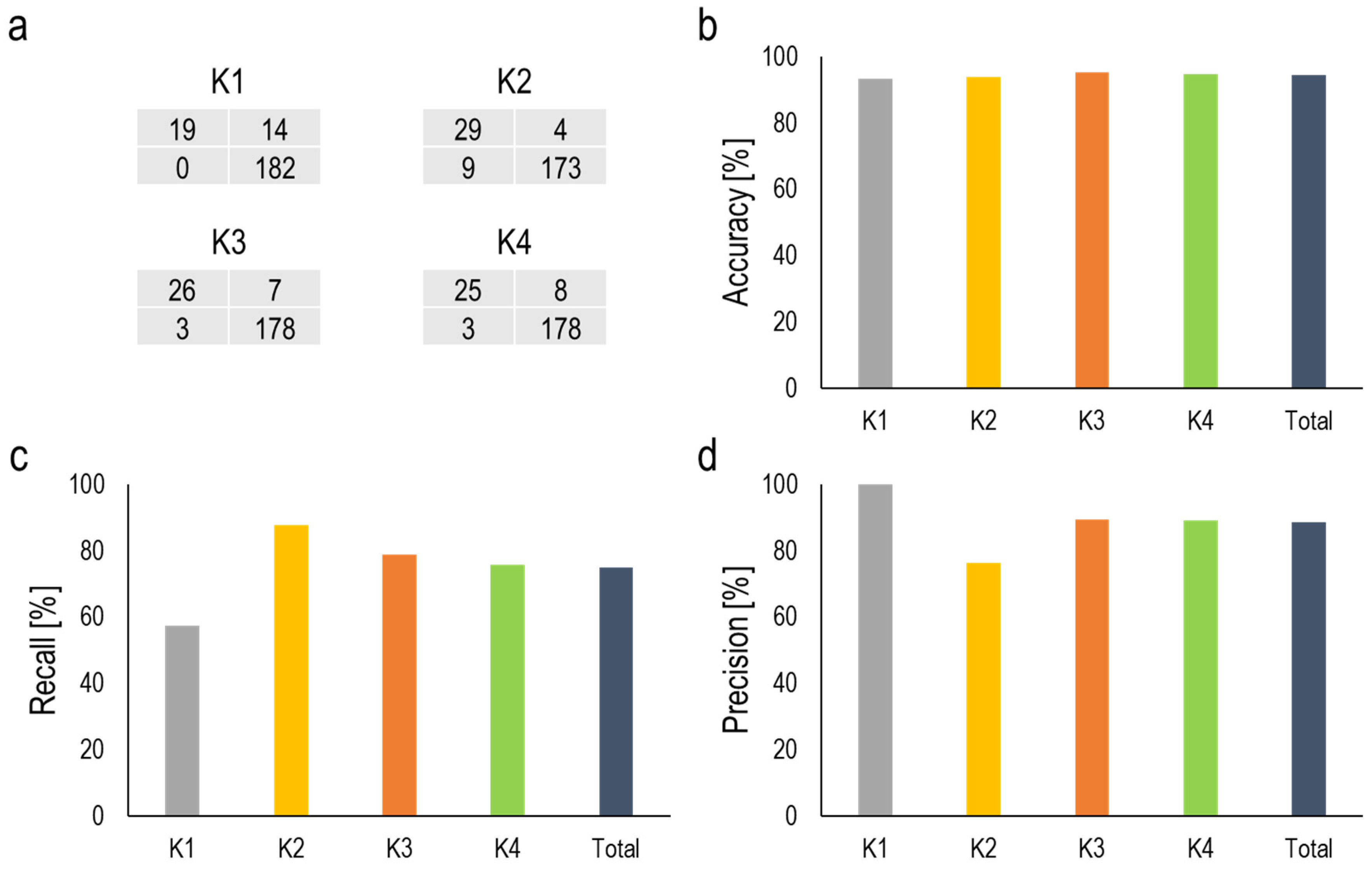
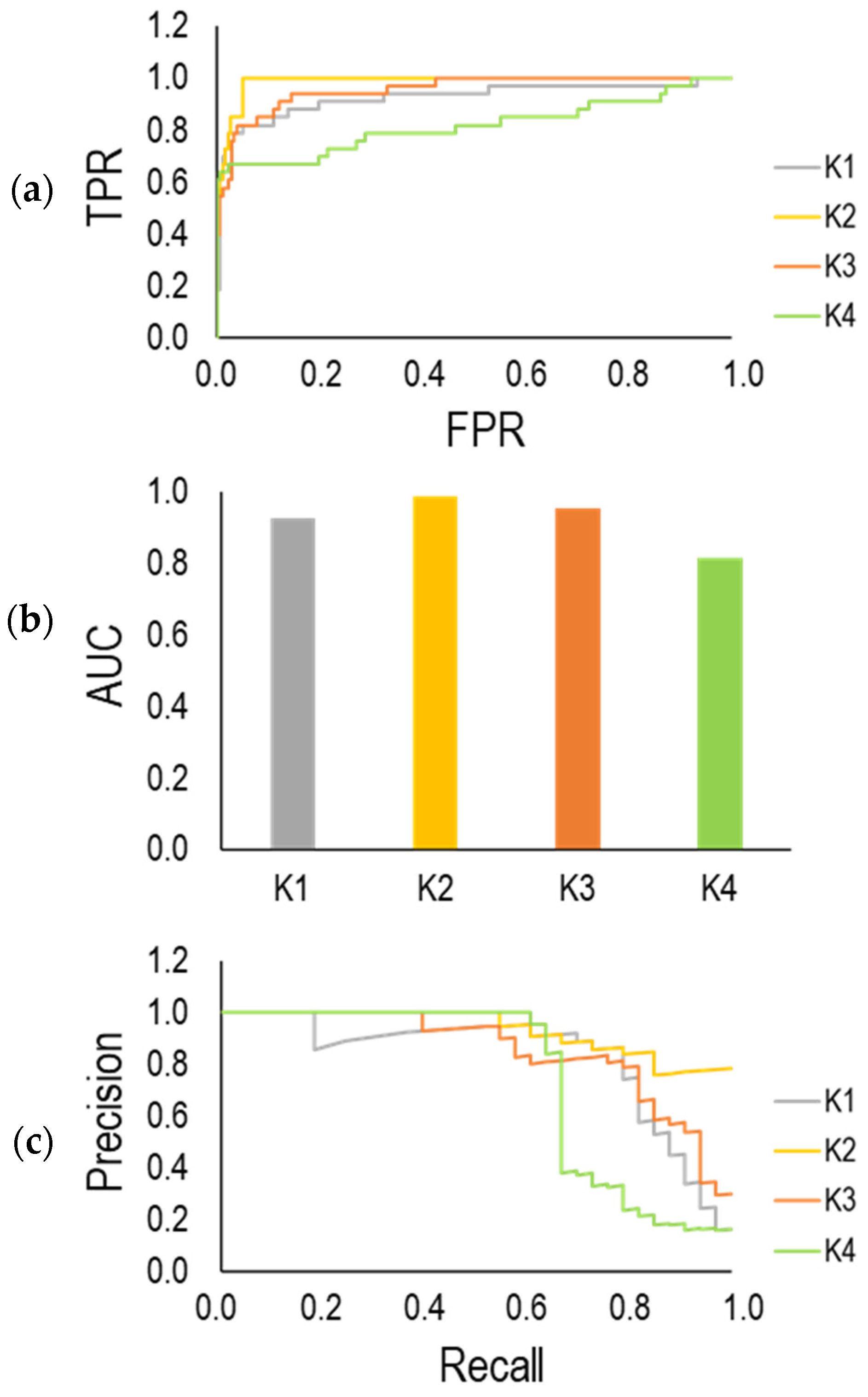
The GASF images were classified into two groups. Group A contained images induced by stable process conditions (no tool breakage and acceptable surface quality). All images belonging to the experimental tests where tool breakage occurred, or the surface quality deteriorated dramatically, were classified in group B. The trained classification CNN model resulted in recall and precision with 75% and 88% values, respectively. According to the evaluation of the CNN model based on ROC and precision-recall curves, the trained models at K = 1, 2, 3 show acceptable performance compared to that at K = 4. Moreover, AUC value for K = 4 is lower than that for others at K = 1, 2, 3. This highlighted that the model suffers from an imbalanced dataset. The extension of the dataset, particularly for group B with a lower number of instances, is required to achieve a better model’s performance.
-
Using the image augmentation technique for oversampling the dataset in the training procedure, the variation of ROC and precision-recall curves between different groups has been reduced. Precision-recall curves show higher precision and recall, and the AUC metric stands over 0.95 in different groups (K = 1, 2, 3 and 4).
-
According to the introduced metrics for the evaluation of the model, the combination of the GAF and CNN classification model for the prediction of critical machining conditions showed a good performance even in the presence of an imbalanced dataset. Improvement of the model in the future can be carried out by expanding the dataset, particularly for collecting more experimental data associated with the critical machining condition. Based on the obtained results, the robustness of time series imaging in combination with the CNN model can also be used in other machining processes to predict unwanted issues and eventually enhance the product’s quality.

Author Contributions

F.H.: Experiment, programming, model development, validation, and writing; B.A.: supervision and editing; A.D.: supervision and editing; R.H.K.: post-process measurements. All authors have read and agreed to the published version of the manuscript.

Funding

Thanks to Ministerium für Wirtschaft, Arbeit und Wohnungsbau Baden-Württemberg for funding the KInCNC Project.

Acknowledgments

Thanks to Company HB microtec for providing the tools/Company Synop Systems for providing ETL program.

Conflicts of Interest

The authors declare no conflict of interest.

References

  1. Ambhore, N.; Kamble, D.; Chinchanikar, S.; Wayal, V. Tool Condition Monitoring System: A Review. Mater. Today Proc. 2015, 2, 3419–3428. [Google Scholar] [CrossRef]
  2. Teti, R.; Jemielniak, K.; O’Donnell, G.; Dornfeld, D. Advanced monitoring of machining operations. CIRP Ann. 2010, 59, 717–739. [Google Scholar] [CrossRef] [Green Version]
  3. Mohanraj, T.; Shankar, S.; Rajasekar, R.; Sakthivel, N.R.; Pramanik, A. Tool condition monitoring techniques in milling process—A review. J. Mater. Res. Technol. 2020, 9, 1032–1042. [Google Scholar] [CrossRef]
  4. Nouri, M.; Fussell, B.K.; Ziniti, B.L.; Linder, E. Real-time tool wear monitoring in milling using a cutting condition independent method. Int. J. Mach. Tools Manuf. 2015, 89, 1–13. [Google Scholar] [CrossRef]
  5. Patra, K.; Jha, A.K.; Szalay, T.; Ranjan, J.; Monostori, L. Artificial neural network based tool condition monitoring in micro mechanical peck drilling using thrust force signals. Precis. Eng. 2017, 48, 279–291. [Google Scholar] [CrossRef]
  6. Drouillet, C.; Karandikar, J.; Nath, C.; Journeaux, A.-C.; El Mansori, M.; Kurfess, T. Tool life predictions in milling using spindle power with the neural network technique. J. Manuf. Process. 2016, 22, 161–168. [Google Scholar] [CrossRef]
  7. Demko, M.; Vrabeľ, M.; Maňková, I.; Ižol, P. Cutting tool monitoring while drilling using internal CNC data. Procedia CIRP 2022, 112, 263–267. [Google Scholar] [CrossRef]
  8. Zhang, X.Y.; Lu, X.; Wang, S.; Wang, W.; Li, W.D. A multi-sensor based online tool condition monitoring system for milling process. Procedia CIRP 2018, 72, 1136–1141. [Google Scholar] [CrossRef]
  9. Hesser, D.F.; Markert, B. Tool wear monitoring of a retrofitted CNC milling machine using artificial neural networks. Manuf. Lett. 2019, 19, 1–4. [Google Scholar] [CrossRef]
  10. Siddhpura, M.; Paurobally, R. A review of chatter vibration research in turning. Int. J. Mach. Tools Manuf. 2012, 61, 27–47. [Google Scholar] [CrossRef]
  11. Hall, S.; Newman, S.T.; Loukaides, E.; Shokrani, A. ConvLSTM deep learning signal prediction for forecasting bending moment for tool condition monitoring. Procedia CIRP 2022, 107, 1071–1076. [Google Scholar] [CrossRef]
  12. Gokulachandran, J.; Bharath Krishna Reddy, B. A study on the usage of current signature for tool condition monitoring of drill bit. Mater. Today Proc. 2021, 46, 4532–4536. [Google Scholar] [CrossRef]
  13. Zhou, C.; Guo, K.; Sun, J. An integrated wireless vibration sensing tool holder for milling tool condition monitoring with singularity analysis. Measurement 2021, 174, 109038. [Google Scholar] [CrossRef]
  14. Ajayram, K.A.; Jegadeeshwaran, R.; Sakthivel, G.; Sivakumar, R.; Patange, A.D. Condition monitoring of carbide and non-carbide coated tool insert using decision tree and random tree—A statistical learning. Mater. Today Proc. 2021, 46, 1201–1209. [Google Scholar] [CrossRef]
  15. González, G.; Schwär, D.; Segebade, E.; Heizmann, M.; Zanger, F. Chip segmentation frequency based strategy for tool condition monitoring during turning of Ti-6Al-4V. Procedia CIRP 2021, 102, 276–280. [Google Scholar] [CrossRef]
  16. Zhang, P.; Gao, D.; Lu, Y.; Ma, Z.; Wang, X.; Song, X. Cutting tool wear monitoring based on a smart toolholder with embedded force and vibration sensors and an improved residual network. Measurement 2022, 199, 111520. [Google Scholar] [CrossRef]
  17. del Olmo, A.; de Lacalle, L.L.; de Pissón, G.M.; Pérez-Salinas, C.; Ealo, J.; Sastoque, L.; Fernandes, M. Tool wear monitoring of high-speed broaching process with carbide tools to reduce production errors. Mech. Syst. Signal Process. 2022, 172, 109003. [Google Scholar] [CrossRef]
  18. Nasir, V.; Dibaji, S.; Alaswad, K.; Cool, J. Tool wear monitoring by ensemble learning and sensor fusion using power, sound, vibration, and AE signals. Manuf. Lett. 2021, 30, 32–38. [Google Scholar] [CrossRef]
  19. Ou, J.; Li, H.; Liu, B.; Peng, D. Deep Transfer Residual Variational Autoencoder with Multi-sensors Fusion for Tool Condition Monitoring in Impeller Machining. Measurement 2022, 204, 112028. [Google Scholar] [CrossRef]
  20. Kuntoğlu, M.; Sağlam, H. Investigation of signal behaviors for sensor fusion with tool condition monitoring system in turning. Measurement 2021, 173, 108582. [Google Scholar] [CrossRef]
  21. Johansson, D.; Hägglund, S.; Bushlya, V.; Ståhl, J.-E. Assessment of Commonly used Tool Life Models in Metal Cutting. Procedia Manuf. 2017, 11, 602–609. [Google Scholar] [CrossRef]
  22. Wang, C.; Bao, Z.; Zhang, P.; Ming, W.; Chen, M. Tool wear evaluation under minimum quantity lubrication by clustering energy of acoustic emission burst signals. Measurement 2019, 138, 256–265. [Google Scholar] [CrossRef]
  23. Tahir, N.; Muhammad, R.; Ghani, J.A.; Nuawi, M.Z.; Haron, C.H.C. Monitoring the flank wear using piezoelectric of rotating tool of main cutting force in end milling. J. Teknol. 2016, 78, 45–51. [Google Scholar] [CrossRef] [Green Version]
  24. Zhou, C.; Guo, K.; Sun, J. Sound singularity analysis for milling tool condition monitoring towards sustainable manufacturing. Mech. Syst. Signal Process. 2021, 157, 107738. [Google Scholar] [CrossRef]
  25. Liu, Y.; Guo, L.; Gao, H.; You, Z.; Ye, Y.; Zhang, B. Machine vision based condition monitoring and fault diagnosis of machine tools using information from machined surface texture: A review. Mech. Syst. Signal Process. 2022, 164, 108068. [Google Scholar] [CrossRef]
  26. Dutta, S.; Pal, S.K.; Sen, R. Progressive tool condition monitoring of end milling from machined surface images. Proc. Inst. Mech. Eng. Part B J. Eng. Manuf. 2018, 232, 251–266. [Google Scholar] [CrossRef]
  27. Lin, W.-J.; Lo, S.-H.; Young, H.-T.; Hung, C.-L. Evaluation of Deep Learning Neural Networks for Surface Roughness Prediction Using Vibration Signal Analysis. Appl. Sci. 2019, 9, 1462. [Google Scholar] [CrossRef] [Green Version]
  28. Bhandari, B.; Park, G. Non-contact surface roughness evaluation of milling surface using CNN-deep learning models. Int. J. Comput. Integr. Manuf. 2022, 1–15. [Google Scholar] [CrossRef]
  29. Rifai, A.P.; Aoyama, H.; Tho, N.H.; Md Dawal, S.Z.; Masruroh, N.A. Evaluation of turned and milled surfaces roughness using convolutional neural network. Measurement 2020, 161, 107860. [Google Scholar] [CrossRef]
  30. Magalhães, L.C.; Magalhães, L.C.; Ramos, J.B.; Moura, L.R.; de Moraes, R.E.N.; Gonçalves, J.B.; Hisatugu, W.H.; Souza, M.T.; de Lacalle, L.N.L.; Ferreira, J.C.E. Conceiving a Digital Twin for a Flexible Manufacturing System. Appl. Sci. 2022, 12, 9864. [Google Scholar] [CrossRef]
  31. Liu, S.; Lu, Y.; Zheng, P.; Shen, H.; Bao, J. Adaptive reconstruction of digital twins for machining systems: A transfer learning approach. Robot. Comput.-Integr. Manuf. 2022, 78, 102390. [Google Scholar] [CrossRef]
  32. Liu, J.; Wen, X.; Zhou, H.; Sheng, S.; Zhao, P.; Liu, X.; Kang, C.; Chen, Y. Digital twin-enabled machining process modeling. Adv. Eng. Inform. 2022, 54, 101737. [Google Scholar] [CrossRef]
  33. Wang, Z.; Oates, T. Imaging Time-Series to Improve Classification and Imputation. arXiv 2015, arXiv:1506.00327v1. [Google Scholar]
  34. Martínez-Arellano, G.; Terrazas, G.; Ratchev, S. Tool wear classification using time series imaging and deep learning. Int. J. Adv. Manuf. Technol. 2019, 104, 3647–3662. [Google Scholar] [CrossRef]
Figure 1. Schematic representation of the integration of the ETL program and AI Model.
Jmmp 06 00145 g001
Figure 2. (a) Experimental setup. (b) Illustration of different axes.
Jmmp 06 00145 g002
Figure 3. (a) Specification of utilized cutting tool; (b) edge 1; (c) edge 2; (d) edge 3.
Jmmp 06 00145 g003
Figure 4. Signals of current, load, power, and torque from different axes and spindle in the slot milling at vc = 50 m/min and fz = 30 µm/tooth.
Jmmp 06 00145 g004
Figure 5. Signals of current, load and torque in different passes before tool breakage at vc = 80 m/min and fz = 20.6 µm/tooth.
Jmmp 06 00145 g005
Figure 6. BUE and tool breakage at vc = 80 m/min and fz = 20.6 µm/tooth (a) edge 1; (b) edge 2; (c) edge 3.
Jmmp 06 00145 g006
Figure 7. (a) Rescaled load signal; (b) polar coordinate mapping of signal; (c) Gramian angular summation field (GASF); (d) Gramian angular difference field (GADF).
Jmmp 06 00145 g007
Figure 8. Extraction of machining area from the GASF image.
Jmmp 06 00145 g008
Figure 9. GASF images at five different milling passes with a new tool and at constant process parameters.
Jmmp 06 00145 g009
Figure 10. Exemplary milled surfaces and their corresponding GASF images; (a) at vc = 75 m/min and fz = 22 µm/tooth in dry machining and (b) at vc = 50 m/min and fz = 30 µm/tooth with oil.
Jmmp 06 00145 g010
Figure 11. Surface roughness values and some exemplary GASF images.
Jmmp 06 00145 g011
Figure 12. Architecture of the CNN model.
Jmmp 06 00145 g012
Figure 13. (a) ReLU function. (b) Sigmoid function.
Jmmp 06 00145 g013
Figure 14. Schematic of confusion matrix.
Jmmp 06 00145 g014
Figure 15. (a) Confusion matrix; (b) accuracy; (c) recall; (d) precision.
Jmmp 06 00145 g015
Figure 16. (a) ROC curve; (b) AUC (area under the ROC curve); (c) precision-recall curve.
Jmmp 06 00145 g016
Figure 17. (a) ROC curve; (b) AUC; (c) precision-recall curve after reducing the imbalance between the number of datasets between groups A and B through oversampling of group B datasets.
Jmmp 06 00145 g017
Table 1. Process parameters.
Cutting Speed vc [m/min]Feed per Tooth fz [µm/tooth]Radial Depth of Cut ae [mm]Axial Depth of Cut ap [mm]Coolant
50–11317–5031Oil/Dry
Publisher’s Note: MDPI stays neutral with regard to jurisdictional claims in published maps and institutional affiliations.

