Constituents Phase Reconstruction through Applied Machine Learning in Nanoindentation Mapping Data of Mortar Surface


Abstract
:1. Introduction
2. Machine Learning Principles
2.1. Supervised and Unsupervised Machine Learning
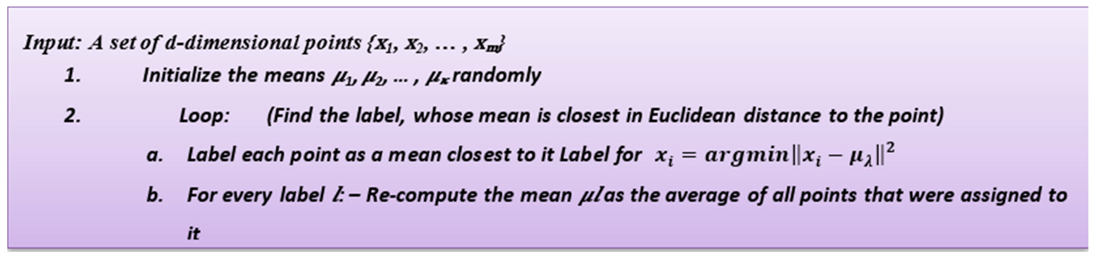
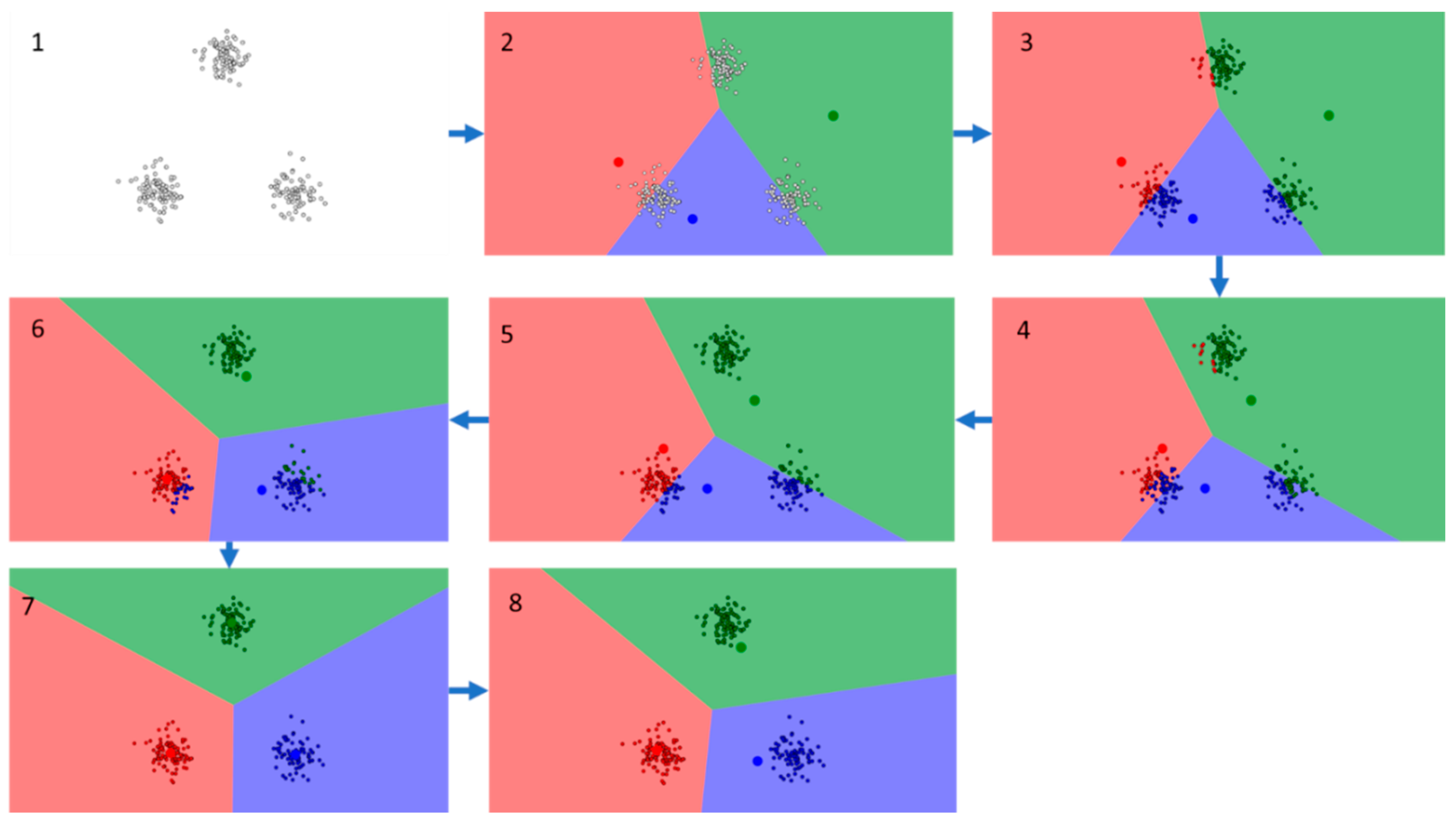
2.2. K-Means Clustering
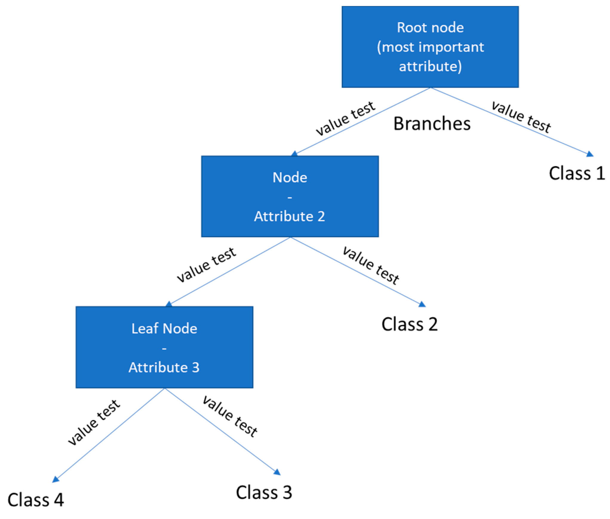
2.3. Decision Trees and Random Forests
3. The Dataset: Experimental Details and Methodology
4. Results and Discussion
5. Conclusions
Author Contributions
Funding
Conflicts of Interest
References
- Tofail, S.A.M.; Koumoulos, E.P.; Bandyopadhyay, A.; Bose, S.; O’Donoghue, L.; Charitidis, C. Additive manufacturing: Scientific and technological challenges, market uptake and opportunities. Mater. Today 2018, 21, 22–37. [Google Scholar] [CrossRef]
- Leatherbarrow, A.; Wu, H. Mechanical behaviour of the constituents inside carbon-fibre/carbon-silicon carbide composites characterised by nano-indentation. J. Eur. Ceram. Soc. 2012, 32, 579–588. [Google Scholar] [CrossRef] [Green Version]
- Urena, A.; Rams, J.; Escalera, M.D.; Sanchez, M. Characterization of interfacial mechanical properties in carbon fiber/aluminium matrix composites by the nanoindentation technique. Compos. Sci. Technol. 2005, 65, 2025–2038. [Google Scholar] [CrossRef]
- Koumoulos, E.P.; Tofail, S.A.M.; Silien, C.; de Felicis, D.; Moscatelli, R.; Dragatogiannis, D.A.; Bemporad, E.; Sebastiani, M.; Charitidis, C.A. Metrology and nano-mechanical tests for nano-manufacturing and nano-bio interface: Challenges & future perspectives. Mater. Des. 2018, 137, 446–462. [Google Scholar] [CrossRef] [Green Version]
- Koumoulos, E.P.; Charitidis, C. Surface analysis and mechanical behaviour mapping of vertically aligned cnt forest array through nanoindentation. Appl. Surf. Sci. 2017, 396, 681–687. [Google Scholar] [CrossRef]
- Koumoulos, E.P.; Charitidis, C.A. Integrity of Carbon-Fibre Epoxy Composites through a Nanomechanical Mapping Protocol towards Quality Assurance. Fibers 2018, 6, 78. [Google Scholar] [CrossRef]
- Koumoulos, E.P.; Jagdale, P.; Kartsonakis, I.A.; Giorcelli, M.; Tagliaferro, A.; Charitidis, C.A. Carbon nanotube/polymer nanocomposites: A study on mechanical integrity through nanoindentation. Polym. Compos. 2015, 36, 1432–1446. [Google Scholar] [CrossRef]
- Charitidis, C.A.; Dragatogiannis, D.A.; Koumoulos, E.P.; Kartsonakis, I.A. Residual stress and deformation mechanism of friction stir welded aluminum alloys by nanoindentation. Mater. Sci. Eng. A 2012, 540, 226–234. [Google Scholar] [CrossRef]
- Charitidis, C.A.; Koumoulos, E.P.; Dragatogiannis, D.A. Nanotribological behavior of carbon-based thin films: Friction and lubricity mechanisms at the nanoscale. Lubricants 2013, 1, 22–47. [Google Scholar] [CrossRef]
- Hu, Z.; Farahikia, M.; Delfanian, F. Fiber bias effect on characterization of carbon fiber-reinforced polymer composites by nanoindentation testing and modeling. J. Compos. Mater. 2015, 49, 3359–3372. [Google Scholar] [CrossRef]
- Maurin, R.; Davies, P.; Baral, N.; Baley, C. Transverse properties of carbon fibres by nano-indentation and micro-mechanics. Appl. Compos. Mater. 2008, 15, 61. [Google Scholar] [CrossRef]
- Hardiman, M.; Vaughan, T.J. A review of key developments and pertinent issues in nanoindentation testing of fibre reinforced plastic microstructures. Compos. Struct. 2017, 180, 782–798. [Google Scholar] [CrossRef]
- Ulm, F.J.; Vandamme, M.; Bobko, C.; Ortega, J.A.; Tai, K.; Ortiz, C. Statistical indentation techniques for hydrated nanocomposites: Concrete, bone, and shale. J. Am. Ceram. Soc. 2007, 90, 2677–2692. [Google Scholar] [CrossRef]
- Sebastiani, M.; Moscatelli, R.; Ridi, F.; Baglioni, P.; Carassitia, F. High-resolution high-speed nanoindentation mapping of cement pastes: Unravelling the effect of microstructure on the mechanical properties of hydrated phases. Mater. Des. 2016, 97, 372–380. [Google Scholar] [CrossRef]
- Allen, A.J.; Thomas, J.J.; Jennings, H.M. Composition and density of nanoscale calcium–silicate–hydrate in cement. Nat. Mater. 2007, 6, 311–316. [Google Scholar] [CrossRef] [PubMed]
- Chiang, W.S.; Ferraro, G.; Fratini, E.; Ridi, F.; Yeh, Y.Q.; Jeng, U.S.; Chen, S.H.; Baglioni, P. Multiscale structure of calcium-and magnesium-silicate-hydrate gels. J. Mater. Chem. A 2014, 2, 12991–12998. [Google Scholar] [CrossRef]
- Shu, X.; Graham, R.K.; Huang, B.; Burdette, E.G. Hybrid effects of carbon fibers on mechanical properties of Portland cement mortar. Mater. Des. 2015, 65, 1222–1228. [Google Scholar] [CrossRef]
- Soto-Pérez, L.; Lopez, V.; Hwang, S.S. Response Surface Methodology to optimize the cement paste mix design: Time-dependent contribution of fly ash and nano-iron oxide as admixtures. Mater. Des. 2015, 86, 22–29. [Google Scholar] [CrossRef]
- Lothenbach, B.; Scrivener, K.; Hooton, R.D. Supplementary cementitious materials. Cem. Concr. Res. 2011, 41, 1244–1256. [Google Scholar] [CrossRef]
- Lee, J.; Mahendra, S.; Alvarez, P.J.J. Nanomaterials in the construction industry: A review of their applications and environmental health and safety considerations. ACS Nano 2010, 4, 3580–3590. [Google Scholar] [CrossRef]
- Chiang, W.C.; Fratini, E.; Ridi, F.; Lim, S.H.; Yeh, Y.Q.; Baglioni, P.; Choi, S.M.; Jeng, U.S.; Chen, S.H. Microstructural changes of globules in calcium–silicate–hydrate gels with and without additives determined by small-angle neutron and X-ray scattering. J. Colloid Interface Sci. 2013, 398, 67–73. [Google Scholar] [CrossRef] [PubMed]
- Hajilar, S.; Shafei, B. Nano-scale investigation of elastic properties of hydrated cement paste constituents using molecular dynamics simulations. Comput. Mater. Sci. 2015, 101, 216–226. [Google Scholar] [CrossRef]
- Nochaiya, T.; Sekine, Y.; Choopun, S.; Chaipanich, A. Microstructure, characterizations, functionality and compressive strength of cement-based materials using zinc oxide nanoparticles as an additive. J. Alloys Compd. 2015, 630, 1–10. [Google Scholar] [CrossRef]
- Le, H.T.; Müller, M.; Siewert, K.; Ludwig, H.M. The mix design for self-compacting high performance concrete containing various mineral admixtures. Mater. Des. 2015, 72, 51–62. [Google Scholar] [CrossRef]
- Constantinides, G.; Ulm, F.J. The effect of two types of CSH on the elasticity of cement-based materials: Results from nanoindentation and micromechanical modeling. Cem. Concr. Res. 2004, 34, 67–80. [Google Scholar] [CrossRef]
- Haoyang, S.; Jinyu, X.; Weibo, R. Experimental study on the dynamic compressive mechanical properties of concrete at elevated temperature. Mater. Des. 2014, 56, 579–588. [Google Scholar] [CrossRef]
- Chen, S.J.; Duan, W.H.; Li, Z.J.; Sui, T.B. New approach for characterisation of mechanical properties of cement paste at micrometre scale. Mater. Des. 2015, 87, 992–995. [Google Scholar] [CrossRef] [Green Version]
- Jiang, J.; Lu, Z.; Niu, Y.; Li, J.; Zhang, Y. Study on the preparation and properties of high-porosity foamed concretes based on ordinary Portland cement. Mater. Des. 2016, 92, 949–959. [Google Scholar] [CrossRef]
- Gao, Y.; Hu, C.; Zhang, Y.; Li, Z.; Pan, J. Characterisation of the interfacial transition zone in mortars by nanoindentation and scanning electron microscope. Mag. Concr. Res. 2018, 70, 965–972. [Google Scholar] [CrossRef]
- Constantinides, G.; Ulm, F.J.; van Vliet, K. On the use of nanoindentation for cementitious materials. Mater. Struct. 2003, 36, 191–196. [Google Scholar] [CrossRef]
- Zadeh, V.Z.; Bobko, C.P. Nano-mechanical properties of internally cured kenaf fiber reinforced concrete using nanoindentation. Cem. Concr. Compos. 2014, 52, 9–17. [Google Scholar] [CrossRef]
- Hintsala, E.D.; Hangen, U.; Stauffer, D.D. High-Throughput Nanoindentation for Statistical and Spatial Property Determination. JOM 2018, 70, 494–503. [Google Scholar] [CrossRef] [Green Version]
- Kusne, A.G.; Gao, T.; Mehta, A.; Ke, L.; Nguyen, M.C.; Ho, K.M.; Takeuchi, I. On-the-fly machine-learning for high-throughput experiments: Search for rare-earth-free permanent magnets. Sci. Rep. 2014, 4, 6367. [Google Scholar] [CrossRef]
- Mueller, T.; Kusne, A.G.; Ramprasad, R. Machine learning in materials science: Recent progress and emerging applications. Rev. Comput. Chem. 2016, 29, 186–273. [Google Scholar]
- Chang, S.; Cohen, T.; Ostdiek, B. What is the machine learning? Phys. Rev. D 2018, 97, 056009. [Google Scholar] [CrossRef] [Green Version]
- Brehmer, J.; Cranmer, K.; Louppe, G.; Pavez, J. Constraining Effective Field Theories with Machine Learning. arXiv 2018, arXiv:1805.00013. [Google Scholar]
- Nieves, J.; Santos, I.; Penya, Y.K.; Rojas, S.; Salazar, M.; Bringas, P.G. Mechanical properties prediction in high-precision foundry production. In Proceedings of the 2009 7th IEEE International Conference on Industrial Informatics, Cardiff, UK, 23–26 June 2009; pp. 31–36. [Google Scholar] [CrossRef]
- Ramprasad, R.; Batra, R.; Pilania, G.; Mannodi-Kanakkithodi, A.; Kim, C. Machine learning in materials informatics: Recent applications and prospects. npj Comput. Mater. 2017, 3, 54. [Google Scholar] [CrossRef]
- Jain, A.K. Data clustering: 50 years beyond K-means. Pattern Recognit. Lett. 2010, 31, 651–666. [Google Scholar] [CrossRef]
- Awad, M.; Khanna, R. Efficient Learning Machines: Theories, Concepts, and Applications for Engineers and System Designers; Apress: New York, NY, USA, 2015. [Google Scholar]
- Quinlan, J.R. Induction of decision trees. Mach. Learn. 1986, 1, 81–106. [Google Scholar] [CrossRef] [Green Version]
- Mannila, H. Data mining: Machine learning, statistics, and databases. In Proceedings of the 8th International Conference on Scientific and Statistical Data Base Management, Stockholm, Sweden, 18–20 June 1996; p. 2. [Google Scholar]
- Koumoulos, E.P.; Dragatogiannis, D.A.; Charitidis, C.A. Nanomechanical properties and deformation mechanism in metals, oxides and alloys. In Nanomechanical Analysis of High-Performance Materials; Springer: Dordrecht, The Netherlands, 2014; pp. 123–152. [Google Scholar]
- Koumoulos, E.P.; Charitidis, C.A.; Papageorgiou, D.P.; Papathanasiou, A.G.; Boudouvis, A.G. Nanomechanical and nanotribological properties of hydrophobic fluorocarbon dielectric coating on tetraethoxysilane for electrowetting applications. Surf. Coat. Technol. 2012, 206, 3823–3831. [Google Scholar] [CrossRef]
- Oliver, W.C.; Pharr, G.M. An improved technique for determining hardness and elastic modulus using load and displacement sensing indentation experiments. J. Mater. Res. 1992, 7, 1564–1583. [Google Scholar] [CrossRef]
- Sneddon, I.N. Boussinesq’s problem for a rigid cone. Math. Proc. Camb. Philos. Soc. 2008, 44, 492–507. [Google Scholar] [CrossRef]
- Huang, L.; Lu, J.; Troyon, M. Nanomechanical properties of nanostructured titanium prepared by SMAT. Surf. Coat. Technol. 2006, 201, 208–213. [Google Scholar] [CrossRef]
- King, R.B. Elastic analysis of some punch problems for a layered medium. Int. J. Solids Struct. 1987, 23, 1657–1664. [Google Scholar] [CrossRef]
- Bei, H.; George, E.P.; Hay, J.L.; Pharr, G.M. Influence of indenter tip geometry on elastic deformation during nanoindentation. Phys. Rev. Lett. 2005, 95, 045501. [Google Scholar] [CrossRef]
- Constantinides, G.; Ulm, F.J. The nanogranular nature of C–S–H. J. Mech. Phys. Solids 2007, 55, 64–90. [Google Scholar] [CrossRef]
- Zhu, W.; Hughes, J.J.; Bicanic, J.N.; Pearce, C.J. Nanoindentation mapping of mechanical properties of cement paste and natural rocks. Mater. Charact. 2017, 58, 1189–1198. [Google Scholar] [CrossRef]
- Hu, C. Nanoindentation as a tool to measure and map mechanical properties of hardened cement pastes. MRS Commun. 2015, 5, 83–87. [Google Scholar] [CrossRef]
- Howind, T.; Hughes, J.J.; Zhu, W.; Puertas, F.; Elizalde, S.G.; Hernandez, M.S.; Dolado, J.S. Mapping of mechanical properties of cement paste microstructures. In Proceedings of the 13th International Congress on the Chemistry of Cement, Madrid, Spain, 3–8 July 2011; p. 309. [Google Scholar]


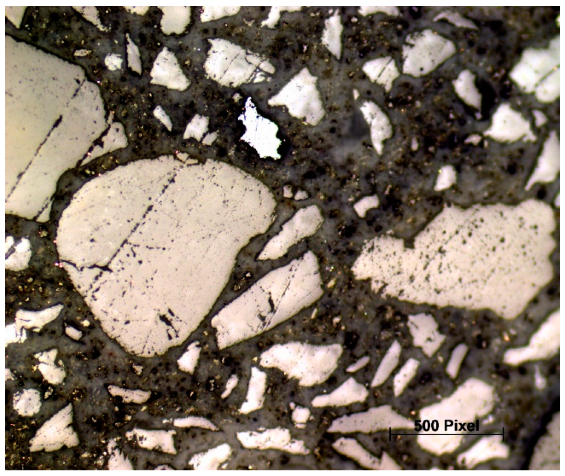
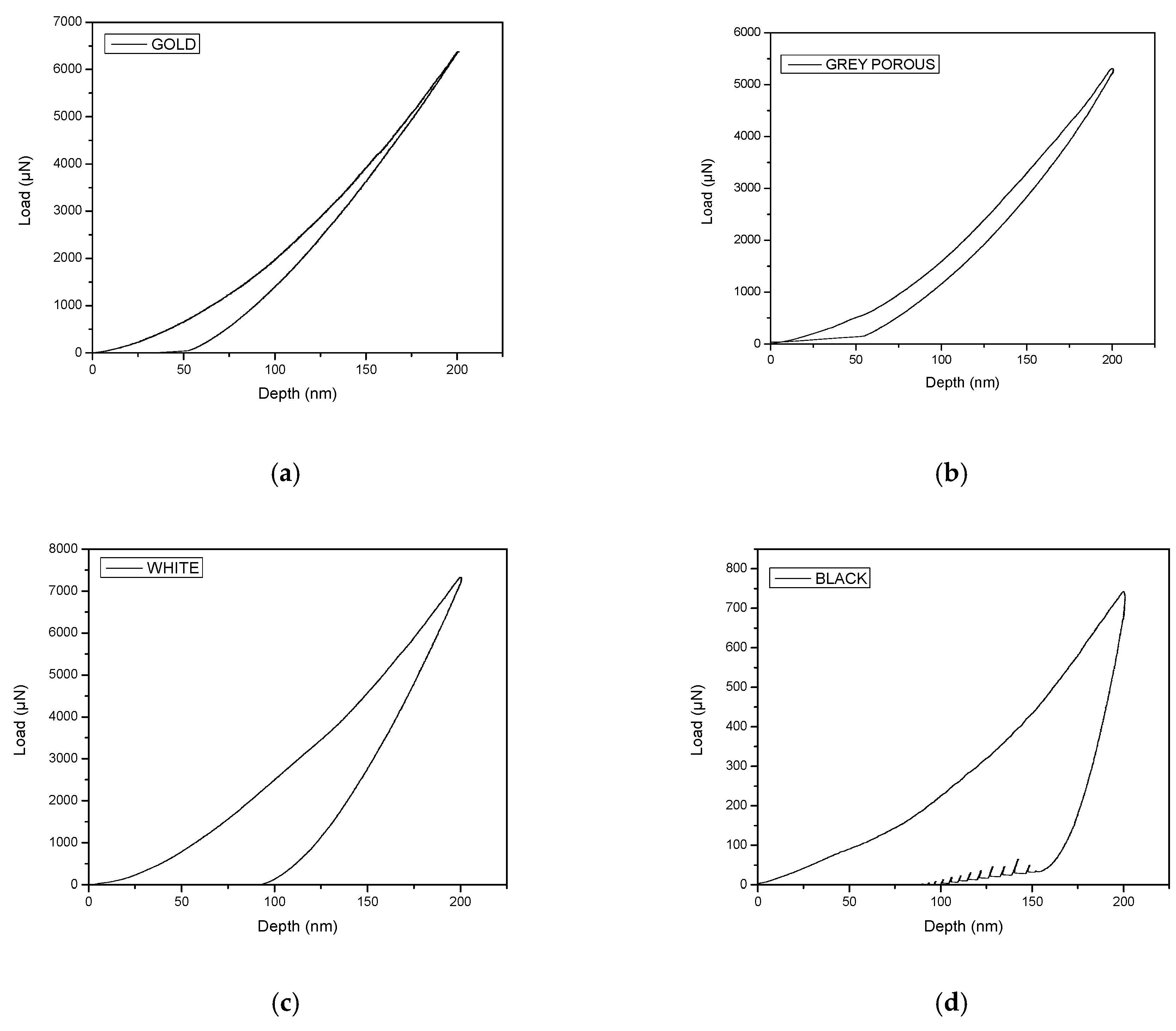
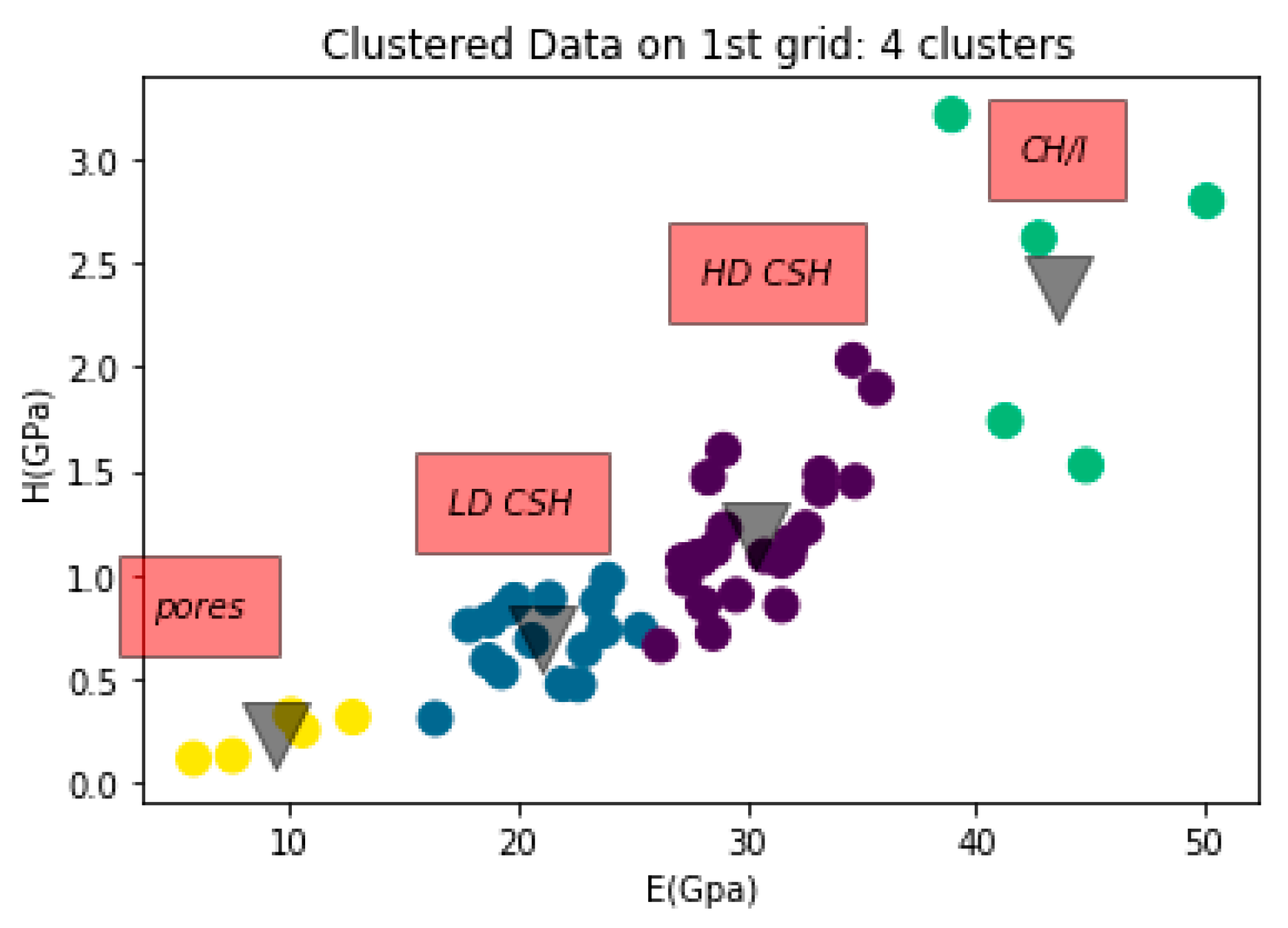
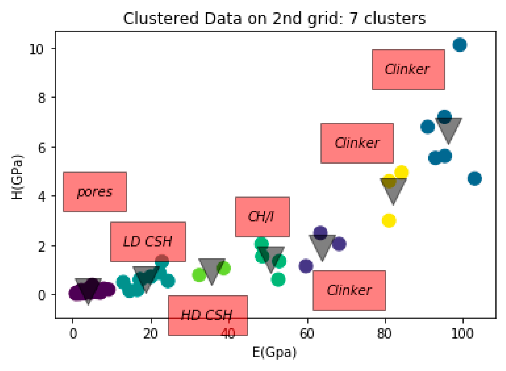
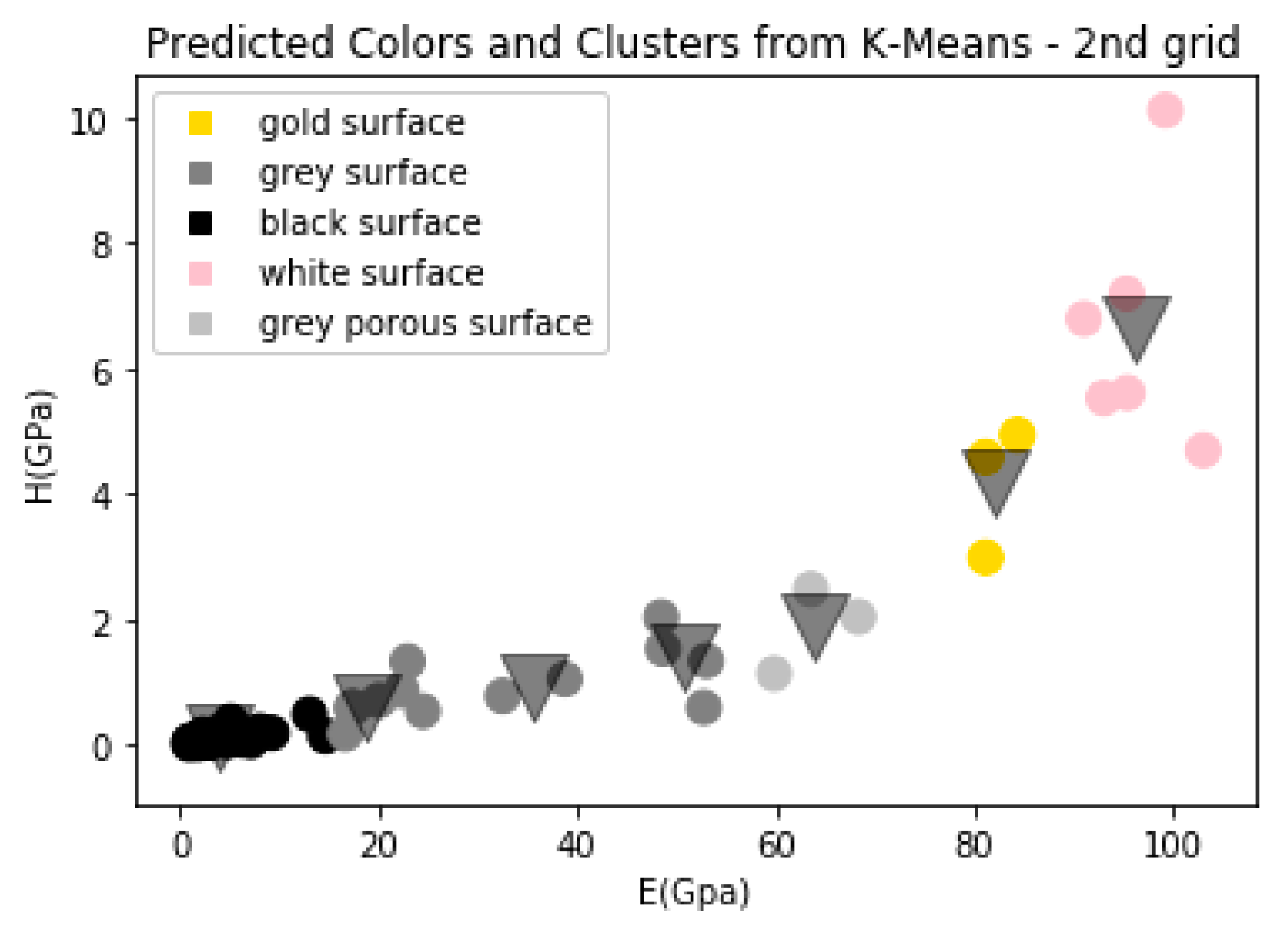
| 1. Cement (grey), containing low/high density C–S–H phase (LD/HD C–S–H) and portlandite (CH) |  |  |
| 2. Clinker (white) |  |  |
| 3. Clinker (left, gold) and Porous clinker (right, grey) |  |  |
| 4. Pores (black) |  |
| Phases | E (GPa) | H (GPa) | ||
|---|---|---|---|---|
| Literature | Cluster (This Work) | Literature | Cluster (This Work) | |
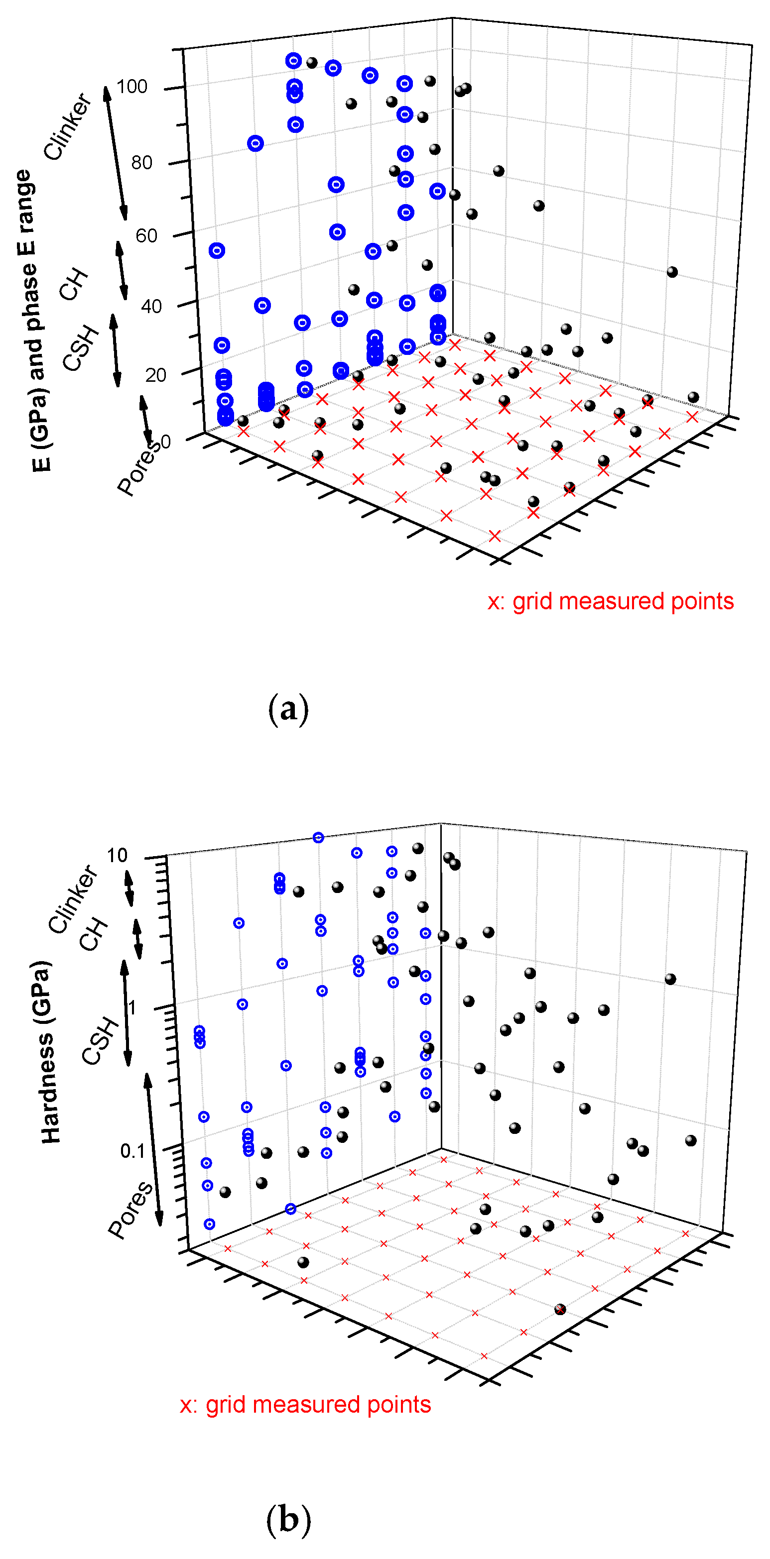
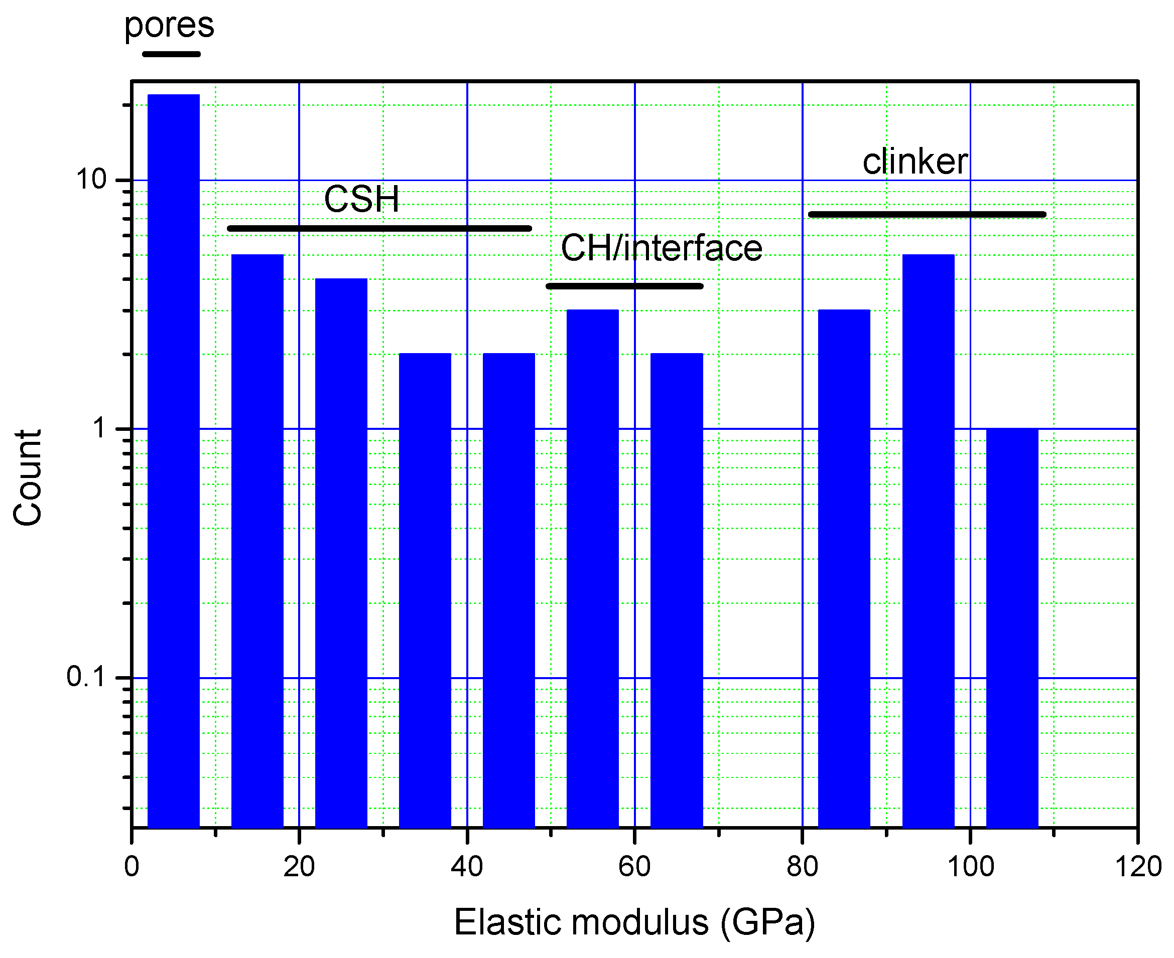
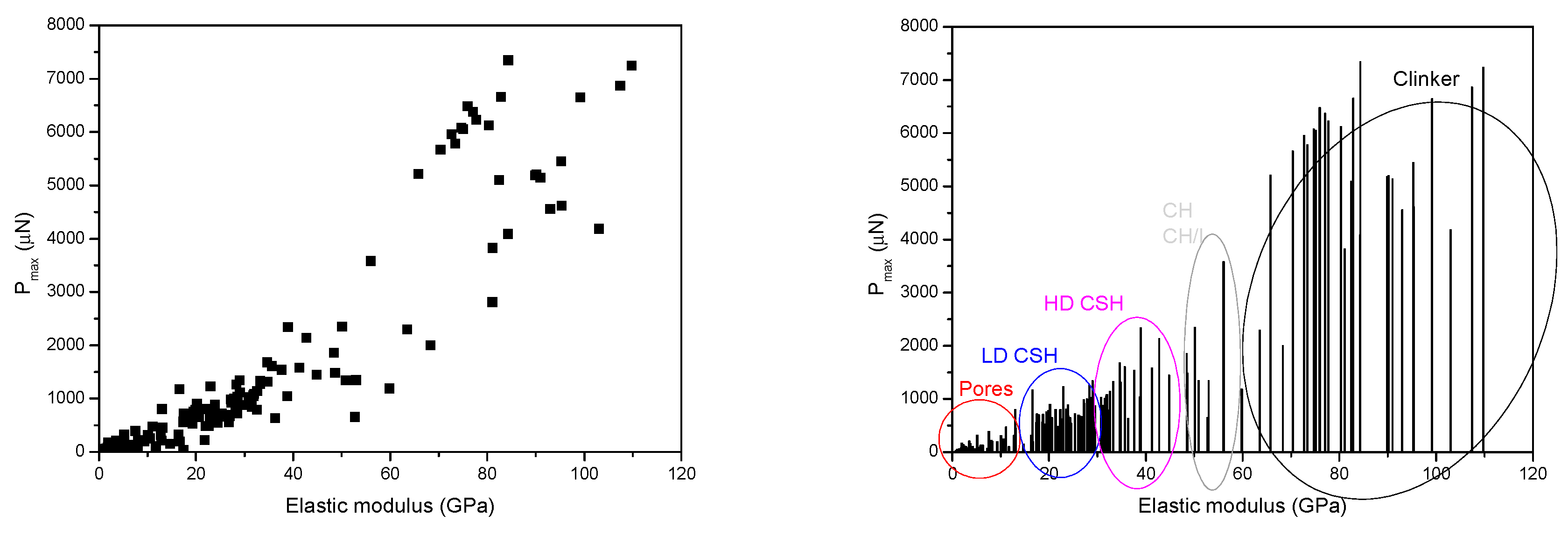
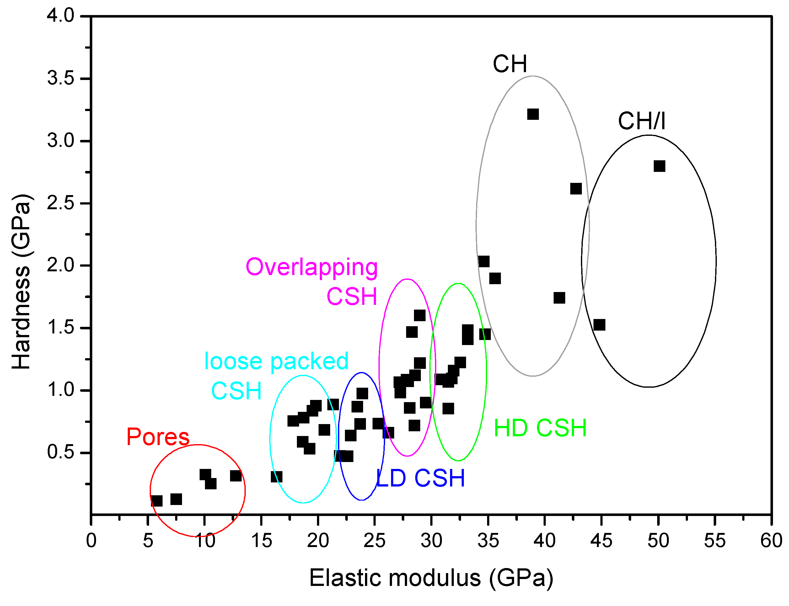
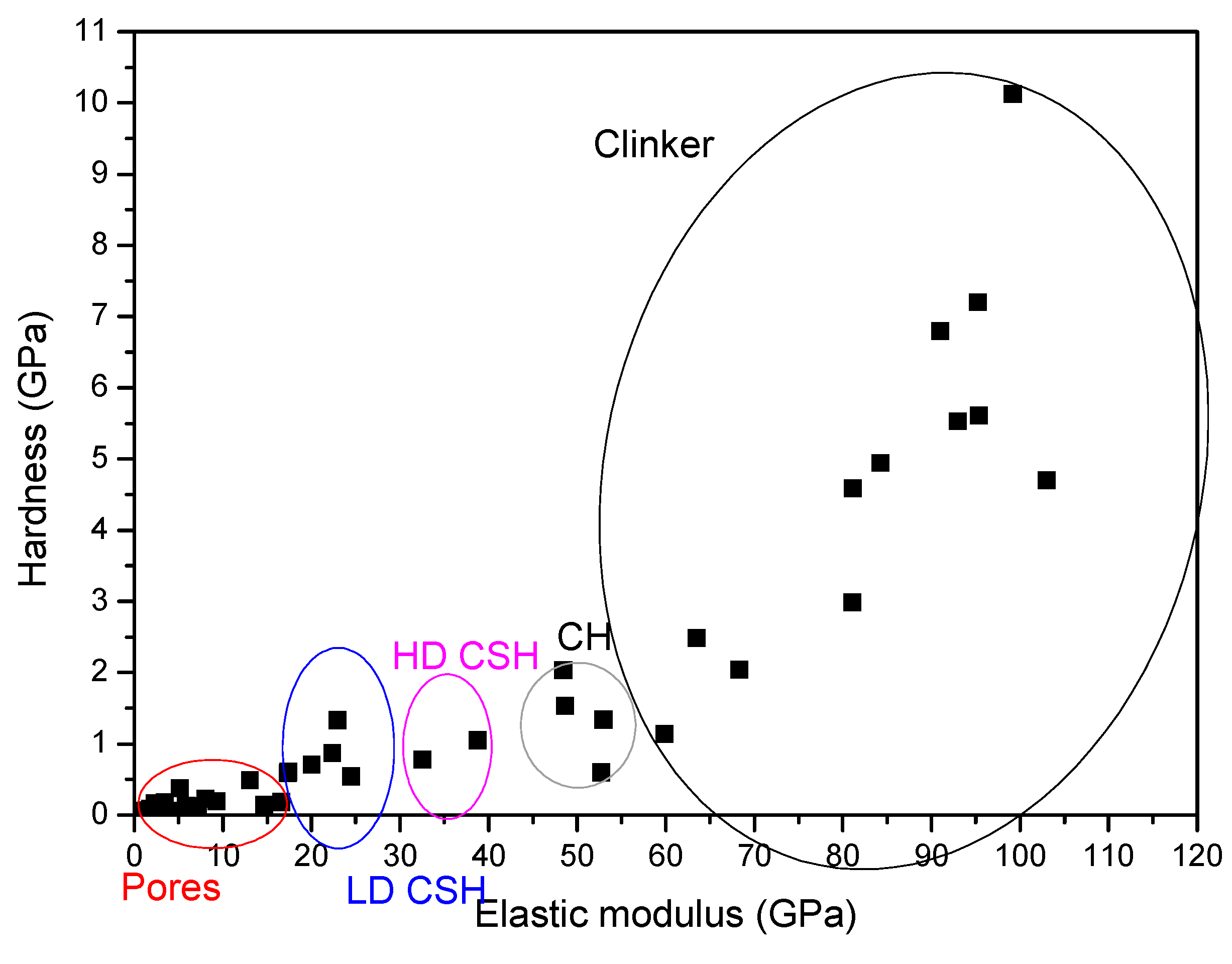
| Pores | 0–13 | 0.2–15 | 0.16–0.18 | 0.1–0.35 |
| LD C-S-H | 13–26 | 16–26 | 0.4–0.8 | 0.4–1.8 |
| HD C-S-H | 26–39 | 26–40 | 0.8–1.25 | 0.4–2.1 |
| CH-CH/I | 35.1–42.9 | 41–58 | 1.31–1.66 | 0.8–3.2 |
| Clinker | - | >60 | - | >1.8 |
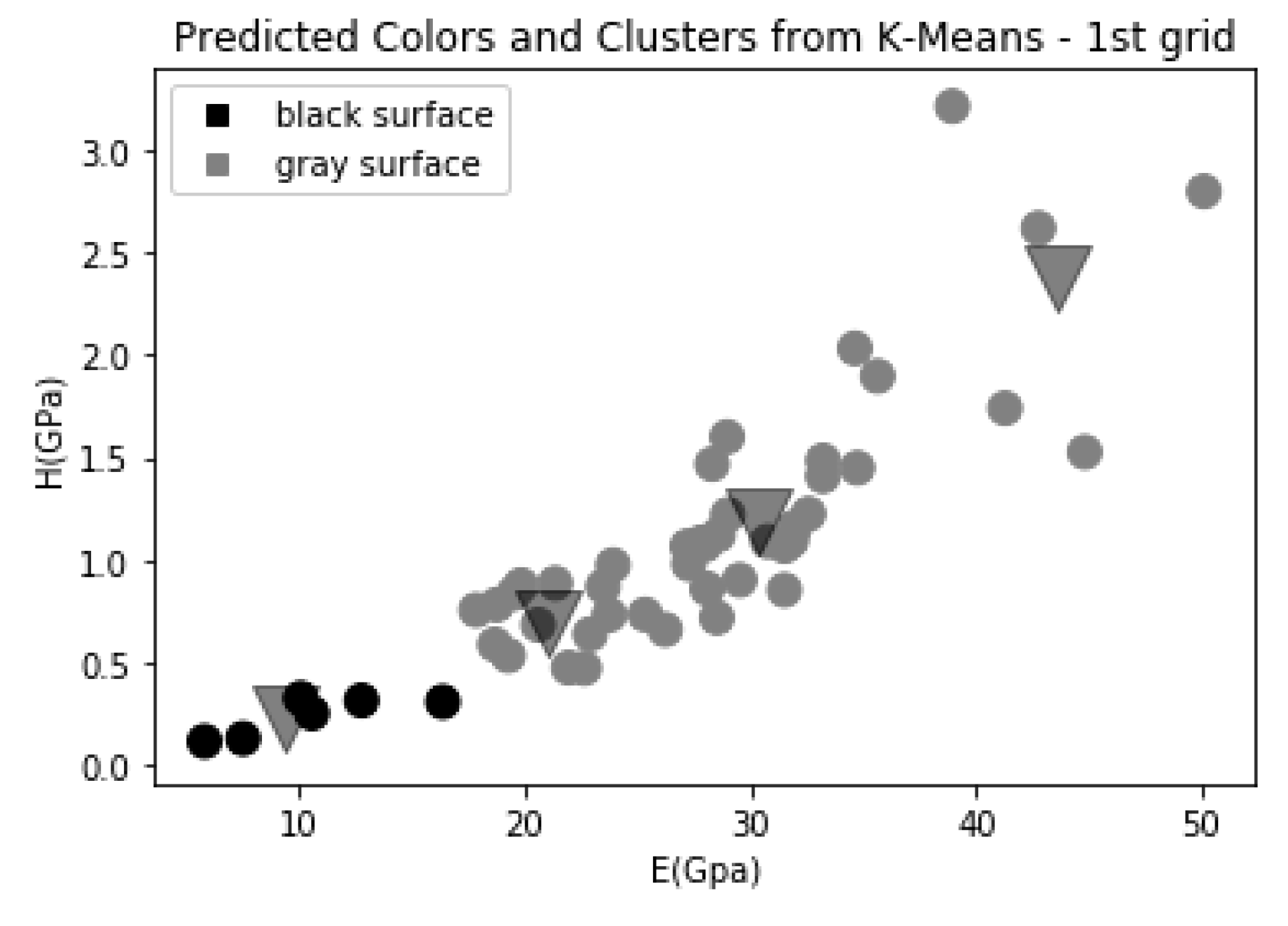
| Surface Colour | E (GPa) | H (GPa) |
|---|---|---|
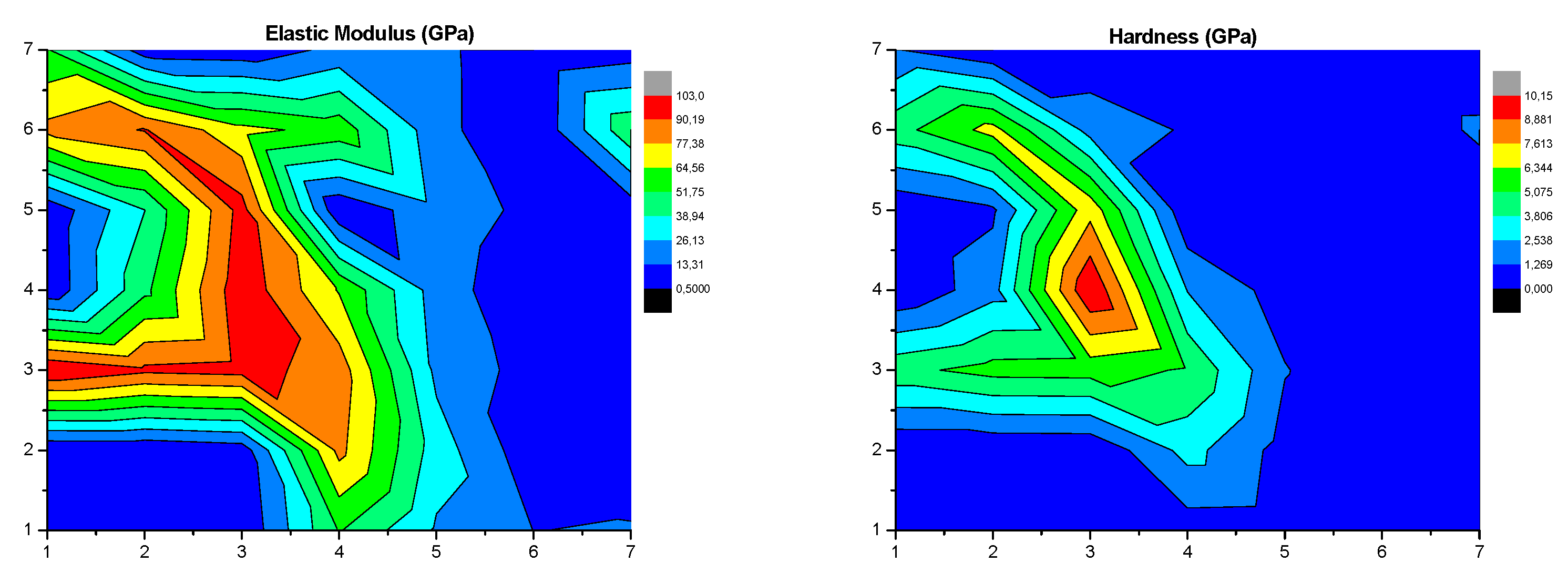
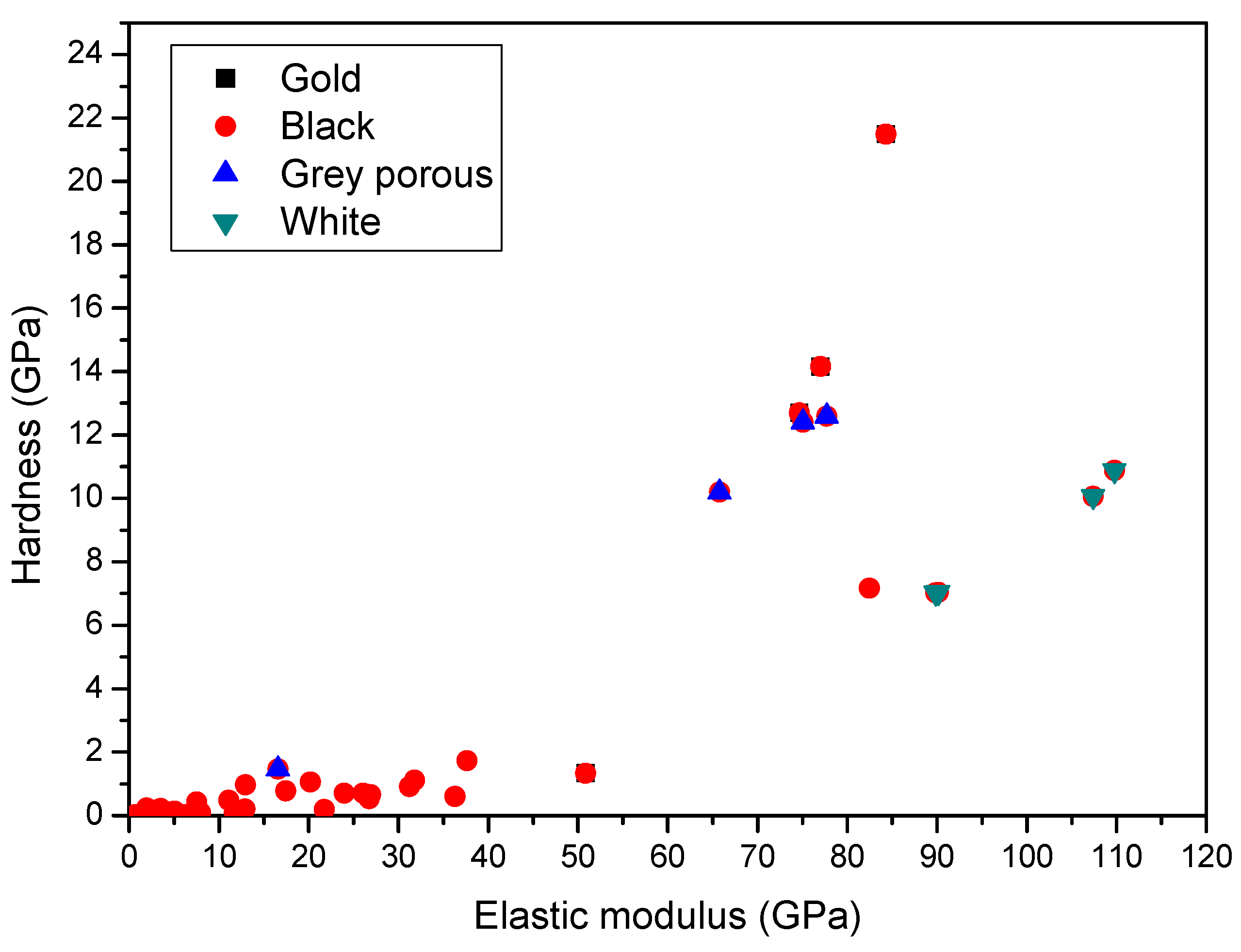
| black | <18 | <0.4 |
| grey | 18–58 | 0.5–3.1 |
| grey porous | 60–71 | 1–2.2 |
| gold | 80–88 | 2.4–5 |
| White | >90 | >4.2 |
© 2019 by the authors. Licensee MDPI, Basel, Switzerland. This article is an open access article distributed under the terms and conditions of the Creative Commons Attribution (CC BY) license (http://creativecommons.org/licenses/by/4.0/).
Share and Cite
Koumoulos, E.P.; Paraskevoudis, K.; Charitidis, C.A. Constituents Phase Reconstruction through Applied Machine Learning in Nanoindentation Mapping Data of Mortar Surface. J. Compos. Sci. 2019, 3, 63. https://0-doi-org.brum.beds.ac.uk/10.3390/jcs3030063
Koumoulos EP, Paraskevoudis K, Charitidis CA. Constituents Phase Reconstruction through Applied Machine Learning in Nanoindentation Mapping Data of Mortar Surface. Journal of Composites Science. 2019; 3(3):63. https://0-doi-org.brum.beds.ac.uk/10.3390/jcs3030063
Chicago/Turabian StyleKoumoulos, Elias P., Konstantinos Paraskevoudis, and Costas A. Charitidis. 2019. "Constituents Phase Reconstruction through Applied Machine Learning in Nanoindentation Mapping Data of Mortar Surface" Journal of Composites Science 3, no. 3: 63. https://0-doi-org.brum.beds.ac.uk/10.3390/jcs3030063