Optimum Design of Carbon/Epoxy Composite Pressure Vessels Including Moisture Effects

Abstract

The main target of the present study is to preserve the structural integrity of the composite pressure vessels (PVs) used in the seawater reverse osmosis (SWRO) desalination plants under internal pressure loading when moisture effects are taken into consideration. Different composite material lay-ups and fiber orientations are considered. In each case, the optimum safe thickness of the PV is found based on the appropriate failure criterion. The PVs are made of carbon/epoxy C/E IM7/977-3 with (±θ)ns lay-up. For verification purposes, PVs made from stainless steel SST 316L and carbon/epoxy C/E AS4/3501-6 are considered and their available results are compared with the predictions of the MATLAB code developed in this study. The study consists of three main cases. The first case considered the PVs materials SST 316L steel and C/E AS4/3501-6 carbon/epoxy composite, without moisturizing effect, with the purpose to verify the results of the developed MATLAB code by comparing with results from the available literature. The second case is concerned with the composite material C/E IM7/977-3, without moisture effects, while the third case included moisture effects on the same material (C/E IM7/977-3). The optimum angles found for C/E AS4/3501-6 is (±55.1)ns and for C/E IM7/977-3 with and without moisture are (±55.8)ns and (±54.0)ns, respectively. The best weight saving of the composite PV, when compared to the steel PV, reached 95.2%.

1. Introduction

A lot of work has been done on the optimization of pressure vessels (PVs), due to their importance in various fields and applications. Using composite materials in PVs is a common way to improve their design and create a lighter, more controlled material behavior. The classical lamination theory (CLT) was used by [1] and [2] to model the composite PV. They have shown that a maximum pressure for the PV can be achieved using higher modulus fibers in the hoop direction and lower modulus fibers in the longitudinal direction. One study proposed a method to design hybrid laminated composite PVs under different loading conditions [3]. A hydrogen PV was investigated and showed the failure under transverse tensile stress using three different techniques, laminate-based, full ply-based and hybrid-based [4]. An optimum lay-up for composite PV was concluded by [5], after analyzing three composite materials with a MATLAB code they programmed. The materials studied were S-glass/epoxy, Kevlar/epoxy and carbon/epoxy (C/E), and their results showed that the optimum lay-up for all composite materials was (±54)ns.

The relation between moisture and temperature effects on the physical aging of polymeric composite IM7/977-3 was studied by using momentary creep tests on off-axis coupon specimens [6]. It was found that the weight gain of the composite material IM7/977-3 reached a steady value of 1.3% after 40 days of immersion.

The desalination solution to supply fresh water in scarce areas is continuously researched and developed [7]. The seawater reverse osmosis (SWRO) desalination plant is an extensively spread technology in desalination. It typically consists of four stages, seawater intake, pretreatment, reverse osmosis system and post-treatment [8]. The current trends in SWRO technologies and future expectations of it were comprehensively reviewed [9]. One aspect of optimizing the SWRO technology is to improve the design of pressure vessels (PVs) used in the filtration units. The filtration unit generally consists of a PV and a membrane element; the membrane is usually fabricated from stainless steel or fiber-reinforced composite materials [10].

A recent study [11], carried out the optimization of SWRO PV for different materials analytically, which was verified using ANSYS software. A comparison was made between stainless steel (SST 316L), the standard material for SWRO PV and different lay-ups and combinations of C/E and E-glass/epoxy (E-g/E). The comparison found out that the optimum lay-ups for E-g/E, C/E and a hybrid E-g/E C/E were (±54)ns, (±55)ns, and (90G/±50C/90G)ns, respectively. Also, the lightest PV was achieved by the C/E composite with the material code AS4/3501-6.

The present work is focused on optimizing the structural integrity of the composite PVs used in SWRO desalination plants, by using different composite material lay-ups and varying the fiber orientation. The previous works did not include the moisture effect when studying the PV in SWRO plants. Moreover, the composite material used in the present study is different from the composite materials used in the previous works, which showed better results.

Building on previous findings in the literature, the optimum lay-up of (±θ)ns for composite PV will be used and a different C/E composite will be investigated. In the first part of the work, the PV will be made from SST 316L and AS4/3501-6 to verify the established MATLAB code and compare with the new results. Second, the composite C/E IM7/977-3 will be investigated and compared with the first study. In both studies, the moisture expansion of PV for being continually filled with water is ignored. In the third and final study, the analysis of composite C/E IM7/977-3 including moisture effects is performed.

2. Methodology

In this study, the optimum fiber orientation and lamination lay-ups are found in order to come up with an allowable PV thickness for a safe design that will guarantee the structural integrity of the vessel during operation under internal pressure loading. Four different sizes of PVs are considered, as shown in

Table 1. Pressure vessel (PV) sizes used in this work.

PV Size	Diameter (mm)	Length (mm)
2.5″	63.5	400
4″	101.6	1000
8″	203.3	1000
16″	406.6	1000

, which are the same sizes found in the literature [11] and adopted here for verification and comparison purposes. A thin-walled analysis is used and only the cylindrical parts of the PVs are considered. The internal pressure in the PVs is chosen to be 8 MPa. The analytical model is developed, and solutions are obtained by establishing a MATLAB code for this purpose. Different materials and loading conditions are utilized and studied in the following three sections (stainless steel SST 316L and composite materials C/E AS4/3501-6 and C/E IM7/977-3). The effect of including moisture is investigated by considering the longitudinal and transverse expansion of the pressure vessel, due to being filled with water. The water content that the studied composite material (C/E IM7/977-3) can absorb was taken from a previous experimental study that showed a steady value of 1.3% moisture difference when immersed for 40 days [6].

The thermal effects are neglected, due to low thermal variation in the working environment [12]. The von Mises failure criterion is used to calculate the minimum allowable steel vessels (SST 316L), while the Tsai–Wu failure criterion is used for the composite vessels (C/E AS4/3501-6 and C/E IM7/977-3).

The composite material lay-ups were selected to be (±θ)ns, where n is the number of basic laminates and s indicate the symmetry of lay-ups. The (±θ)ns lay-up provides good results when compared to other common lay-ups, as reported in some previous works [4].

2.1. Case 1: SST 316L and C/E AS4/3501-6, Without Moisture Effects

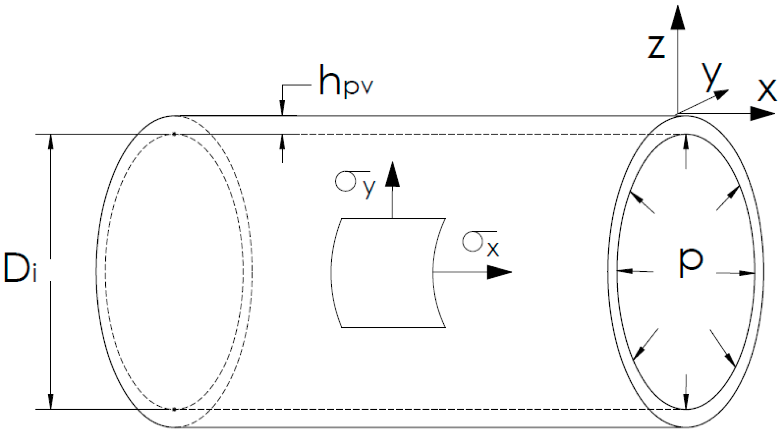
The purpose of this case is to verify the analysis procedure and the MATLAB code by comparing its results with the previous work [11]. Two analyses were performed, in the first one, the four PV sizes made from stainless steel SST 316L (Figure 1) was subjected to 8 MPa internal pressure. Moisture effect is not taken into consideration in this case. The material is considered isotropic and linearly elastic with the properties shown in

Table 2. Properties of stainless steel SST 316L [11].

Property	Value
Density (kg/m3)	7750
Young’s modulus (GPa)	193
Poisson’s ratio	0.31
Tensile yield strength (MPa)	207
Tensile ultimate strength (MPa)	586

.

The relations for axial and hoop stresses, σ_x and σ_y respectively [13], to a thin-walled cylinder, are as follows:

$${\mathsf{\sigma }}_{\mathrm{x}}=\frac{{\mathrm{pD}}_{\mathrm{i}}}{4{\mathrm{h}}_{\mathrm{PV}}}$$

(1)

$${\mathsf{\sigma }}_{\mathrm{y}}=\frac{{\mathrm{pD}}_{\mathrm{i}}}{2{\mathrm{h}}_{\mathrm{PV}}}$$

(2)

where, p is the internal water pressure, in MPa; D_i is the internal diameter of the PV, in mm; h_PV is the thickness of the PV cylindrical part, in mm

By utilizing the principal stresses with the von Mises yield criterion, the following relation for stainless steel SST 316L PV thickness can be found:

$${\mathrm{h}}_{\mathrm{PV}}=\frac{\sqrt{3}{\mathrm{pD}}_{\mathrm{i}}}{4{\mathrm{S}}_{\mathrm{ty}}}{\mathrm{SF}}_{\mathrm{all}}$$

(3)

where, ${\mathrm{S}}_{\mathrm{ty}}$ is the tensile yield strength of SST 316L, in MPa; ${\mathrm{SF}}_{\mathrm{all}}$ is the allowable safety factor of the PV, in mm.

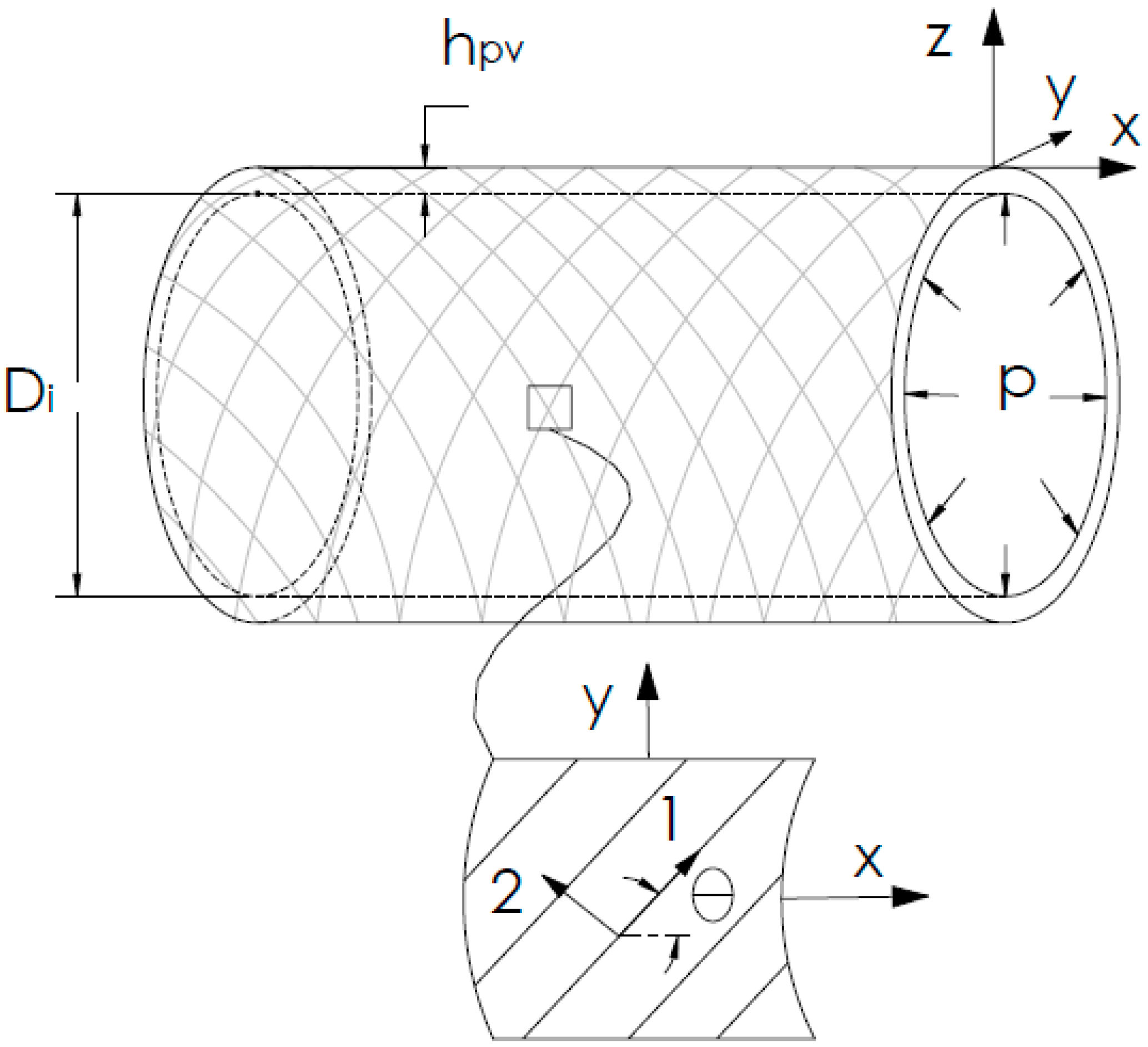
In the second analysis, the four PVs shown in Figure 2 are made from C/E AS4/3501-6 composite with the properties shown in

Table 3. Properties of the composite materials used in this work, from [15]. Properties indicated by (*) are found using composite micromechanics relations from [14]. C/E: carbon/epoxy.

Properties	C/E AS4/3501-6	C/E IM7/977-3
Fiber volume fraction	0.63	0.45
Density (kg/m3)	1580	1610
Longitudinal modulus (GPa)	142	190
Transverse modulus (GPa)	10.3	9.9
In-plane shear modulus (GPa)	7.2	7.8
Major Poisson’s ratio	0.27	0.35
Longitudinal tensile strength (MPa)	2280	3250
Transverse tensile strength (MPa)	57	62
In-plane shear strength (MPa)	71	75
Longitudinal compressive strength (MPa)	620	1590
Transverse compressive strength (MPa)	128	200
Longitudinal moisture expansion coefficient	0.01	*0.0081
Transverse moisture expansion coefficient	0.20	*0.5575

. The same loading conditions used in SST 316L PV were applied in this analysis as well.

The composite C/E AS4/3501-6 vessel is fabricated from a laminate that consists of four laminae, each with a thickness of 0.2 mm and a lay-up of (±θ)ns. The analytical procedure used to create the basic laminate model is performed using the classical lamination theory (CLT), [14].

Each lamina is considered to be orthotropic and linearly elastic. The stress–strain relations for a thin lamina (a plane stress condition) are:

$$\left[\begin{array}{c}{\mathsf{\epsilon }}_1\\ {\mathsf{\epsilon }}_2\\ {\mathsf{\gamma }}_{12}\end{array}\right]=\left[\begin{array}{ccc}\frac{1}{{\mathrm{E}}_1}& -\frac{{\mathsf{\nu }}_{21}}{{\mathrm{E}}_2}& 0\\ -\frac{{\mathsf{\nu }}_{12}}{{\mathrm{E}}_1}& \frac{1}{{\mathrm{E}}_2}& 0\\ 0& 0& \frac{1}{{\mathrm{G}}_{12}}\end{array}\right]\left[\begin{array}{c}{\mathsf{\sigma }}_1\\ {\mathsf{\sigma }}_2\\ {\mathsf{\tau }}_{12}\end{array}\right]$$

(4)

where ${\mathsf{\epsilon }}_{\mathrm{i}}$ is the normal strain in the i axis; ${\mathsf{\gamma }}_{\mathrm{ij}}$ is the shear strain in the i–j plane; ${\mathrm{E}}_{\mathrm{i}}$ is the modulus of elasticity in the i axis, in GPa; ${\mathrm{G}}_{\mathrm{ij}}$ is the shear modulus in the i–j plane, in GPa; ${\mathsf{\nu }}_{\mathrm{ij}}$ is the Poisson’s ratio for the i–j plane;${\mathsf{\sigma }}_{\mathrm{i}}$ is the normal stress in the i axis, in MPa; ${\mathsf{\tau }}_{\mathrm{ij}}$ is the shear stress in the i–j plane, in MPa.

Equation (4) can also be written as:

$$\left[\begin{array}{c}{\mathsf{\sigma }}_1\\ {\mathsf{\sigma }}_2\\ {\mathsf{\tau }}_{12}\end{array}\right]=\left[\begin{array}{ccc}{\mathrm{Q}}_{11}& {\mathrm{Q}}_{12}& 0\\ {\mathrm{Q}}_{12}& {\mathrm{Q}}_{22}& 0\\ 0& 0& {\mathrm{Q}}_{66}\end{array}\right]\left[\begin{array}{c}{\mathsf{\epsilon }}_1\\ {\mathsf{\epsilon }}_2\\ {\mathsf{\gamma }}_{12}\end{array}\right]\mathrm{or}\left[{\mathsf{\sigma }}_{1,2}\right]=\left[{\mathrm{Q}}_{1,2,6}\right]\left[{\mathsf{\epsilon }}_{1,2}\right]$$

(5)

where $Q_{ij}$ are the stiffness components in the i–j direction, and can be found using:

$$\begin{gathered} {\mathrm{Q}}_{11}=\frac{{\mathrm{E}}_1}{1-{\mathsf{\nu }}_{12}{\mathsf{\nu }}_{21}}, \\ {\mathrm{Q}}_{12}=\frac{{\mathsf{\nu }}_{12}{\mathrm{E}}_2}{1-{\mathsf{\nu }}_{12}{\mathsf{\nu }}_{21}}, \\ {\mathrm{Q}}_{22}=\frac{{\mathrm{E}}_2}{1-{\mathsf{\nu }}_{12}{\mathsf{\nu }}_{21}}, \\ {\mathrm{Q}}_{66}={\mathrm{G}}_{12}. \end{gathered}$$

(6)

The transformation between the lamina’s material principle axes (1, 2) to the global axes of the laminate (x, y) can be done with the following:

$$\left[\begin{array}{c}{\mathsf{\sigma }}_1\\ {\mathsf{\sigma }}_2\\ {\mathsf{\tau }}_{12}\end{array}\right]=T\left[\begin{array}{c}{\mathsf{\sigma }}_{\mathrm{x}}\\ {\mathsf{\sigma }}_{\mathrm{y}}\\ {\mathsf{\tau }}_{\mathrm{xy}}\end{array}\right]$$

(7)

$$\left[\begin{array}{c}{\mathsf{\epsilon }}_1\\ {\mathsf{\epsilon }}_2\\ \frac{1}{2}{\mathsf{\gamma }}_{12}\end{array}\right]=T\left[\begin{array}{c}{\mathsf{\epsilon }}_{\mathrm{x}}\\ {\mathsf{\epsilon }}_{\mathrm{y}}\\ \frac{1}{2}{\mathsf{\gamma }}_{\mathrm{xy}}\end{array}\right]$$

(8)

where T is the transformation matrix and can be determined as follow:

$$T=\left[\begin{array}{ccc}{\mathrm{C}}^2& {\mathrm{S}}^2& 2\mathrm{CS}\\ {\mathrm{S}}^2& {\mathrm{C}}^2& -2\mathrm{CS}\\ -\mathrm{CS}& \mathrm{CS}& {\mathrm{C}}^2-{\mathrm{S}}^2\end{array}\right], \mathrm{C}=\cos \mathsf{\theta },\mathrm{S}=\sin \mathsf{\theta }$$

(9)

Utilizing Equations (5) to (9) leads to:

$$\left[\begin{array}{c}{\mathsf{\sigma }}_{\mathrm{x}}\\ {\mathsf{\sigma }}_{\mathrm{y}}\\ {\mathsf{\tau }}_{\mathrm{xy}}\end{array}\right]=\left[\begin{array}{ccc}{\overline{\mathrm{Q}}}_{11}& {\overline{\mathrm{Q}}}_{12}& {\overline{\mathrm{Q}}}_{16}\\ {\overline{\mathrm{Q}}}_{12}& {\overline{\mathrm{Q}}}_{22}& {\overline{\mathrm{Q}}}_{26}\\ {\overline{\mathrm{Q}}}_{16}& {\overline{\mathrm{Q}}}_{26}& {\overline{\mathrm{Q}}}_{66}\end{array}\right]\left[\begin{array}{c}{\mathsf{\epsilon }}_{\mathrm{x}}\\ {\mathsf{\epsilon }}_{\mathrm{y}}\\ {\mathsf{\gamma }}_{\mathrm{xy}}\end{array}\right] \mathrm{or}\left[{\mathsf{\sigma }}_{\mathrm{x},\mathrm{y}}\right]=[{\overline{\mathrm{Q}}}_{1,2,6}]\left[{\mathsf{\epsilon }}_{\mathrm{x},\mathrm{y}}\right]$$

(10)

where $\overline{Q}$_1,2,6 are the elements of the transformed reduced stiffness matrix and are given by:

$$\begin{array}{l}{\overline{\mathrm{Q}}}_{11}={\mathrm{Q}}_{11}{\mathrm{C}}^4+{\mathrm{Q}}_{22}{\mathrm{S}}^4+2({\mathrm{Q}}_{12}+2{\mathrm{Q}}_{66}){\mathrm{S}}^2{\mathrm{C}}^2\\ {\overline{\mathrm{Q}}}_{12}=({\mathrm{Q}}_{11}+{\mathrm{Q}}_{22}-4{\mathrm{Q}}_{66}){\mathrm{S}}^2{\mathrm{C}}^2+{\mathrm{Q}}_{12}\left({\mathrm{S}}^2+{\mathrm{C}}^4\right)\\ {\overline{\mathrm{Q}}}_{22}={\mathrm{Q}}_{11}{\mathrm{S}}^4+{\mathrm{Q}}_{22}{\mathrm{C}}^4+2({\mathrm{Q}}_{12}+2{\mathrm{Q}}_{66}){\mathrm{S}}^2{\mathrm{C}}^2\\ {\overline{\mathrm{Q}}}_{16}=({\mathrm{Q}}_{11}-{\mathrm{Q}}_{12}-2{\mathrm{Q}}_{66}){\mathrm{C}}^3\mathrm{S}-({\mathrm{Q}}_{22}-{\mathrm{Q}}_{12}-2{\mathrm{Q}}_{66}){\mathrm{S}}^3\mathrm{C}\\ {\overline{\mathrm{Q}}}_{26}=({\mathrm{Q}}_{11}-{\mathrm{Q}}_{12}-2{\mathrm{Q}}_{66}){\mathrm{S}}^3\mathrm{C}-({\mathrm{Q}}_{22}-{\mathrm{Q}}_{12}-2{\mathrm{Q}}_{66}){\mathrm{C}}^3\mathrm{S}\\ {\overline{\mathrm{Q}}}_{66}=({\mathrm{Q}}_{11}+{\mathrm{Q}}_{22}-2{\mathrm{Q}}_{12}-2{\mathrm{Q}}_{66}){\mathrm{S}}^2{\mathrm{C}}^2+{\mathrm{Q}}_{66}\left({\mathrm{S}}^4+{\mathrm{C}}^4\right)\end{array}$$

(11)

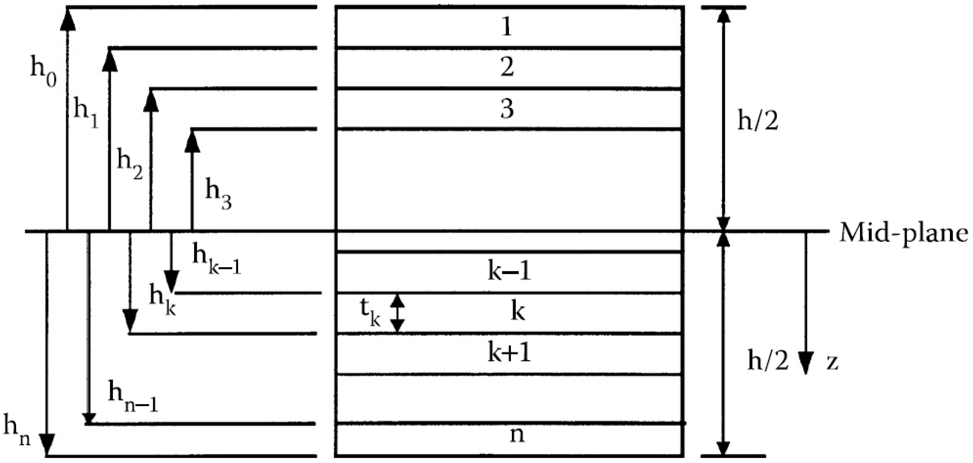
After finding the $\overline{Q}$ matrix for all four laminae in the basic laminate, the surface position of each lamina from the laminate mid-plane can be determined. The position from the laminate mid-plane to the bottom surface of each lamina is h_k, and can be found using:

$${\mathrm{h}}_{\mathrm{k}}=-\frac{\mathrm{h}}{2}+{\sum }_1^{\mathrm{k}}\mathrm{t} \left(\mathrm{bottom}\mathrm{surface}\right)$$

(12)

where h is the laminate thickness (the basic laminate thickness, 0.8 mm in this work), ${\mathrm{t}}_{\mathrm{k}}$ is the thickness of each lamina (taken as 0.2 mm) and k refers to the number of the lamina (Figure 3).

Knowing $\overline{Q}$ and ${\mathrm{h}}_{\mathrm{k}}$_, the extensional, the coupling and bending stiffness matrices, A, B and D respectively, can be found from the following:

$$\begin{gathered} {\mathrm{A}}_{\mathrm{ij}}={\sum }_{\mathrm{k}=1}^{\mathrm{n}}{[{\mathrm{Q}¯}_{\mathrm{ij}}]}_{\mathrm{k}}\left({\mathrm{h}}_{\mathrm{k}}-{\mathrm{h}}_{\mathrm{k}-1}\right),\mathrm{i}=1,2,6;\mathrm{j}=1,2,6 \\ {\mathrm{B}}_{\mathrm{ij}}=\frac{1}{2}{\sum }_{\mathrm{k}=1}^{\mathrm{n}}{[{\mathrm{Q}¯}_{\mathrm{ij}}]}_{\mathrm{k}}\left({\mathrm{h}}_{\mathrm{k}}^2-{\mathrm{h}}_{\mathrm{k}-1}^2\right),\mathrm{i}=1,2,6;\mathrm{j}=1,2,6 \\ {\mathrm{D}}_{\mathrm{ij}}=\frac{1}{3}{{\displaystyle \sum }}_{\mathrm{k}=1}^{\mathrm{n}}{[{\mathrm{Q}¯}_{\mathrm{ij}}]}_{\mathrm{k}}\left({\mathrm{h}}_{\mathrm{k}}^3-{\mathrm{h}}_{\mathrm{k}-1}^3\right),\mathrm{i}=1,2,6;\mathrm{j}=1,2,6 \end{gathered}$$

(13)

The mid-plane strains ${{\epsilon }_{x,y}}^{\mathbf{0}}$ and curvatures ${\mathsf{\kappa }}_{x,y}$ can be solved for from:

$$\left[\begin{array}{c}{\mathrm{N}}_{\mathrm{x}}\\ {\mathrm{N}}_{\mathrm{y}}\\ \begin{array}{c}{\mathrm{N}}_{\mathrm{xy}}\\ {\mathrm{M}}_{\mathrm{x}}\\ \begin{array}{c}{\mathrm{M}}_{\mathrm{y}}\\ {\mathrm{M}}_{\mathrm{xy}}\end{array}\end{array}\end{array}\right]=\left[\begin{array}{cccccc}{\mathrm{A}}_{11}& {\mathrm{A}}_{12}& {\mathrm{A}}_{16}& {\mathrm{B}}_{11}& {\mathrm{B}}_{12}& {\mathrm{B}}_{16}\\ {\mathrm{A}}_{12}& {\mathrm{A}}_{22}& {\mathrm{A}}_{26}& {\mathrm{B}}_{12}& {\mathrm{B}}_{22}& {\mathrm{B}}_{26}\\ {\mathrm{A}}_{16}& {\mathrm{A}}_{26}& {\mathrm{A}}_{66}& {\mathrm{B}}_{16}& {\mathrm{B}}_{26}& {\mathrm{B}}_{66}\\ {\mathrm{B}}_{11}& {\mathrm{B}}_{12}& {\mathrm{B}}_{16}& {\mathrm{D}}_{11}& {\mathrm{D}}_{12}& {\mathrm{D}}_{16}\\ {\mathrm{B}}_{12}& {\mathrm{B}}_{22}& {\mathrm{B}}_{26}& {\mathrm{D}}_{12}& {\mathrm{D}}_{22}& {\mathrm{D}}_{26}\\ {\mathrm{B}}_{16}& {\mathrm{B}}_{26}& {\mathrm{B}}_{66}& {\mathrm{D}}_{16}& {\mathrm{D}}_{26}& {\mathrm{D}}_{66}\end{array}\right]\left[\begin{array}{c}{\mathsf{\epsilon }}_{\mathrm{x}}^0\\ {\mathsf{\epsilon }}_{\mathrm{x}}^0\\ \begin{array}{c}{\mathsf{\gamma }}_{\mathrm{xy}}^0\\ {\mathsf{\kappa }}_{\mathrm{x}}\\ \begin{array}{c}{\mathsf{\kappa }}_{\mathrm{y}}\\ {\mathsf{\kappa }}_{\mathrm{xy}}\end{array}\end{array}\end{array}\right],\mathrm{or}\left[\begin{array}{c}\mathrm{N}\\ \mathrm{M}\end{array}\right]=\left[\begin{array}{cc}A& B\\ B& D\end{array}\right]\left[\begin{array}{c}{\mathsf{\epsilon }}^0\\ \mathsf{\kappa }\end{array}\right]$$

(14)

where N_xy and M_xy are the resultant forces and moments per unit length in the laminate, in N/m and N, respectively. The loads in this study are:

$${\mathrm{N}}_{\mathrm{x}}={\mathsf{\sigma }}_{\mathrm{x}}\mathrm{h}=\frac{{\mathrm{pD}}_{\mathrm{i}}}{4},{\mathrm{N}}_{\mathrm{y}}={\mathsf{\sigma }}_{\mathrm{y}}\mathrm{h}=\frac{{\mathrm{pD}}_{\mathrm{i}}}{2}$$

(15)

Using the assumptions of CLT the laminate strains at any location across the thickness can be determined, by the following:

$$\left[\begin{array}{c}{\mathsf{\epsilon }}_{\mathrm{x}}\\ {\mathsf{\epsilon }}_{\mathrm{y}}\\ {\mathsf{\gamma }}_{\mathrm{xy}}\end{array}\right]=\left[\begin{array}{c}{{\mathsf{\epsilon }}_{\mathrm{x}}}^0\\ {{\mathsf{\epsilon }}_{\mathrm{y}}}^0\\ {{\mathsf{\gamma }}_{\mathrm{xy}}}^0\end{array}\right]+\mathrm{z}\left[\begin{array}{c}{\mathsf{\kappa }}_{\mathrm{x}}\\ {\mathsf{\kappa }}_{\mathrm{y}}\\ {\mathsf{\kappa }}_{\mathrm{xy}}\end{array}\right]$$

(16)

where z is the location we wish to find the strains and is measured from the laminate mid-plane, following the same coordinate as shown in Figure 3.

Utilizing Equations (6) to (16), the local stresses and strains at the top and bottom surfaces of each lamina can be found as functions of the fiber angles only,$\mathbf{\sigma }{\left(\theta \right)}_{ij}$ and $\mathbf{\epsilon }\left(\theta \right)$_ij, respectively.

The failure criterion of Tsai–Wu is used to determine the safety factor (SF ($\mathsf{\theta }$)) for all the local stresses previously found, eight $\mathbf{\sigma }{\left(\theta \right)}_{ij}$ and eight SF ($\mathsf{\theta }$), which relate to the top and bottom of each of the four laminas in the basic laminate. According to the Tsai–Wu failure, the lamina will fail if Equation (17) is violated.

$${\mathrm{H}}_1{\mathsf{\sigma }}_1+{\mathrm{H}}_2{\mathsf{\sigma }}_2+{\mathrm{H}}_6{\mathsf{\tau }}_{12}+{\mathrm{H}}_{11}{\mathsf{\sigma }}_1^2+{\mathrm{H}}_{22}{\mathsf{\sigma }}_2^2+{\mathrm{H}}_{66}{\mathsf{\tau }}_{12}^2+2{\mathrm{H}}_{12}{\mathsf{\sigma }}_1{\mathsf{\sigma }}_2<1$$

(17)

where:

$$\begin{gathered} {\mathrm{H}}_1=\frac{1}{{\mathrm{S}}_{1\mathrm{TU}}}-\frac{1}{{\mathrm{S}}_{1\mathrm{CU}}},{\mathrm{H}}_2=\frac{1}{{\mathrm{S}}_{2\mathrm{TU}}}-\frac{1}{{\mathrm{S}}_{2\mathrm{CU}}},{\mathrm{H}}_{11}=\frac{1}{{\mathrm{S}}_{1\mathrm{TU}}{\mathrm{S}}_{1\mathrm{CU}}} \\ {\mathrm{H}}_{22}=\frac{1}{{\mathrm{S}}_{2\mathrm{TU}}{\mathrm{S}}_{2\mathrm{CU}}},{\mathrm{H}}_{12}=-\frac{1}{2}\sqrt{{\mathrm{H}}_{11}{\mathrm{H}}_{22}},{\mathrm{H}}_{66}=\frac{1}{{({\mathrm{S}}_{12\mathrm{SU}})}^2} \end{gathered}$$

(18)

where the subscripts of S refer to the fiber longitudinal direction, fiber transverse direction, tensile strength, compression strength, shear strength and ultimate strength of the lamina, respectively.

Using the first ply failure approach, only the minimum of the eight safety factor functions (${\mathrm{SF}}_{\min }$ ($\mathsf{\theta }$)) is considered. Knowing ${\mathrm{SF}}_{\min }$ ($\mathsf{\theta }$), the allowable thickness ${\mathrm{h}}_{\mathrm{all}}$($\mathsf{\theta }$) can be found by

$${\mathrm{h}}_{\mathrm{all}}\left(\mathsf{\theta }\right)=\frac{{\mathrm{SF}}_{\mathrm{all}}}{{\mathrm{SF}}_{\min }\left(\mathsf{\theta }\right)}\mathrm{h}$$

(19)

where ${\mathrm{SF}}_{\mathrm{all}}$ is the allowable (or design) safety factor (taken as two).

Solving for entries of θ from 0° to 90°, the relation between the PV allowable thickness ${\mathrm{h}}_{\mathrm{all}}\left(\mathsf{\theta }\right)$ and fiber angles θ can be realized. The minimum allowable thickness $({\mathrm{h}}_{\mathrm{all}.\min })$ and the optimum fiber angle $\left({\mathsf{\theta }}_{\mathrm{opt}}\right)$ can then be determined.

The design of ${\mathrm{h}}_{\mathrm{PV}}$ cannot be completed using the value for ${\mathrm{h}}_{\mathrm{all}.\min }$. In order for the analysis procedure to hold, only an integer number of the basic laminates can be added. Thus, the number of required basic laminates n can be found by

$$\mathrm{n}=\frac{{\mathrm{SF}}_{\mathrm{all}}}{{\mathrm{SF}}_{\min }}$$

(20)

where n is approximated to the highest integer. The final pressure vessel thickness can be calculated as follows:

$${\mathrm{h}}_{\mathrm{PV}}=\mathrm{n}\mathrm{x}\mathrm{h}$$

(21)

2.2. Case 2: C/E IM7/977-3, Without Moisture Effects

The composite PV made of C/E IM7/977-3 subjected to the same loading conditions in case 1 (internal pressure = 8 MPa and no moisture effects) is solved analytically. The same analysis procedure and material assumptions of case 1 are used. The composite material properties can be found in Table 3.

The purpose of this study was to increase the specific strength of the PV and compare the solution with case 1.

2.3. Case 3: C/E IM7/977-3, Including Moisture Effects

In this case, the moisture effect is taken into consideration in the analysis of C/E IM7/977-3 PV. In order to include the moisture effects, the longitudinal and transverse moisture expansion coefficients for the composite material should be known as ${\mathsf{\beta }}_1$ and ${\mathsf{\beta }}_2$, respectively. The values of ${\mathsf{\beta }}_1$ and ${\mathsf{\beta }}_2$ for C/E IM7/977-3 are 0.0081 and 0.5575, respectively (using the equations of micromechanical analysis). The micromechanical relations used are [14]:

$${\mathsf{\beta }}_1=\frac{{\mathrm{E}}_{\mathrm{m}}{\mathsf{\rho }}_{\mathrm{c}}}{{\mathrm{E}}_1{\mathsf{\rho }}_{\mathrm{m}}}{\mathsf{\beta }}_{\mathrm{m}}$$

(22)

$${\mathsf{\beta }}_2=\left(1+{\mathsf{\nu }}_{\mathrm{m}}\right)\frac{{\mathsf{\rho }}_{\mathrm{c}}}{{\mathsf{\rho }}_{\mathrm{m}}}{\mathsf{\beta }}_{\mathrm{m}}-{\mathsf{\beta }}_1{\mathsf{\nu }}_{12}$$

(23)

where ${\mathrm{E}}_{\mathrm{m}}$ is the matrix modulus of elasticity, 3.7 GPa for epoxy 977-3 [15]; ${\mathsf{\rho }}_{\mathrm{m}}$ is the matrix density, 1280 kg/m³ for epoxy 977-3 [15]; ${\mathsf{\beta }}_{\mathrm{m}}$ is the matrix moisture expansion coefficient, 0.33 assumed [14]; ${\mathsf{\rho }}_{\mathrm{c}}$ is the composite density, 1610 kg/m for C/E IM7/977-3 [15]; ${\mathsf{\nu }}_{\mathrm{m}}$ is the matrix Poisson’s ratio, 0.35 for epoxy 977-3 [15]; ${\mathsf{\nu }}_{12}$ is the composite major Poisson’s ratio, 0.35 for C/E IM7/977-3 [15].

The change in the moisture content of the composite ($\Delta \mathrm{C}$) determines how much water the composite material has absorbed during a set of time. In a previous study by [6], the effect of immersing a C/E IM7/977-3 specimen in water was experimented. It was found that after 40 days of immersing in water, it reached a steady state value of 1.3% weight gain ($\Delta \mathrm{C}=1.3\%$).

To include the moisture effect in the analysis, all the previous mathematical formulation from Equation (4) to Equation (13) should be performed. In Equation (14) another term is added to account for the resistance created by the bonds between the laminae, the resistance occurs due to different moisture expansion response in each lamina. Equation (14) in compact notation becomes:

$$\left[\begin{array}{c}{\mathrm{N}}^{\mathrm{C}}\\ {\mathrm{M}}^{\mathrm{C}}\end{array}\right]+\left[\begin{array}{c}\mathrm{N}\\ \mathrm{M}\end{array}\right]=\left[\begin{array}{cc}A& B\\ B& D\end{array}\right]\left[\begin{array}{c}{\mathsf{\epsilon }}^0\\ \mathsf{\kappa }\end{array}\right]$$

(24)

where,

$$\left[{\mathrm{N}}^{\mathrm{C}}\right]=\left[\begin{array}{c}{\mathrm{N}}_{\mathrm{x}}^{\mathrm{C}}\\ {\mathrm{N}}_{\mathrm{y}}^{\mathrm{C}}\\ {\mathrm{N}}_{\mathrm{xy}}^{\mathrm{C}}\end{array}\right]=\Delta \mathrm{C}{\displaystyle \sum }_{\mathrm{k}=1}^{\mathrm{n}}{\left[\begin{array}{ccc}{\overline{\mathrm{Q}}}_{11}& {\overline{\mathrm{Q}}}_{12}& {\overline{\mathrm{Q}}}_{16}\\ {\overline{\mathrm{Q}}}_{12}& {\overline{\mathrm{Q}}}_{22}& {\overline{\mathrm{Q}}}_{26}\\ {\overline{\mathrm{Q}}}_{16}& {\overline{\mathrm{Q}}}_{26}& {\overline{\mathrm{Q}}}_{66}\end{array}\right]}_{\mathrm{k}}{\left[\begin{array}{c}{\mathsf{\beta }}_{\mathrm{x}}\\ {\mathsf{\beta }}_{\mathrm{y}}\\ {\mathsf{\beta }}_{\mathrm{xy}}\end{array}\right]}_{\mathrm{k}}\left({\mathrm{h}}_{\mathrm{k}}-{\mathrm{h}}_{\mathrm{k}-1}\right)$$

(25)

$$\left[{\mathrm{M}}^{\mathrm{C}}\right]=\left[\begin{array}{c}{\mathrm{M}}_{\mathrm{x}}^{\mathrm{C}}\\ {\mathrm{M}}_{\mathrm{y}}^{\mathrm{C}}\\ {\mathrm{M}}_{\mathrm{xy}}^{\mathrm{C}}\end{array}\right]=\frac{1}{2}\Delta \mathrm{C}{\displaystyle \sum }_{\mathrm{k}=1}^{\mathrm{n}}{\left[\begin{array}{ccc}{\overline{\mathrm{Q}}}_{11}& {\overline{\mathrm{Q}}}_{12}& {\overline{\mathrm{Q}}}_{16}\\ {\overline{\mathrm{Q}}}_{12}& {\overline{\mathrm{Q}}}_{22}& {\overline{\mathrm{Q}}}_{26}\\ {\overline{\mathrm{Q}}}_{16}& {\overline{\mathrm{Q}}}_{26}& {\overline{\mathrm{Q}}}_{66}\end{array}\right]}_{\mathrm{k}}{\left[\begin{array}{c}{\mathsf{\beta }}_{\mathrm{x}}\\ {\mathsf{\beta }}_{\mathrm{y}}\\ {\mathsf{\beta }}_{\mathrm{xy}}\end{array}\right]}_{\mathrm{k}}\left({\mathrm{h}}_{\mathrm{k}}^2-{\mathrm{h}}_{\mathrm{k}-1}^2\right)$$

(26)

and,

$$\left[\begin{array}{c}{\mathsf{\beta }}_{\mathrm{x}}\\ {\mathsf{\beta }}_{\mathrm{y}}\\ {\mathsf{\beta }}_{\mathrm{xy}}/2\end{array}\right]=T^{-1}\left[\begin{array}{c}{\mathsf{\beta }}_1\\ {\mathsf{\beta }}_2\\ 0\end{array}\right]$$

(27)

Using Equations (15) and (16), the actual global strains can be found in any location across the thickness ${\epsilon }_{x,y}$. To determine the mechanical strains that induce stresses in the material, the following relations are used:

$${\left[\begin{array}{c}{\mathsf{\epsilon }}_{\mathrm{x}}^{\mathrm{M}}\\ {\mathsf{\epsilon }}_{\mathrm{y}}^{\mathrm{M}}\\ {\mathsf{\gamma }}_{\mathrm{xy}}^{\mathrm{M}}\end{array}\right]}_{\mathrm{k}}=\left[\begin{array}{c}{\mathsf{\epsilon }}_{\mathrm{x}}\\ {\mathsf{\epsilon }}_{\mathrm{y}}\\ {\mathsf{\gamma }}_{\mathrm{xy}}\end{array}\right]-{\left[\begin{array}{c}{\mathsf{\epsilon }}_{\mathrm{x}}^{\mathrm{C}}\\ {\mathsf{\epsilon }}_{\mathrm{y}}^{\mathrm{C}}\\ {\mathsf{\gamma }}_{\mathrm{xy}}^{\mathrm{C}}\end{array}\right]}_{\mathrm{k}} ,{\left[\begin{array}{c}{\mathsf{\epsilon }}_{\mathrm{x}}^{\mathrm{C}}\\ {\mathsf{\epsilon }}_{\mathrm{y}}^{\mathrm{C}}\\ {\mathsf{\gamma }}_{\mathrm{xy}}^{\mathrm{C}}\end{array}\right]}_{\mathrm{k}}=\Delta \mathrm{C}{\left[\begin{array}{c}{\mathsf{\beta }}_{\mathrm{x}}\\ {\mathsf{\beta }}_{\mathrm{y}}\\ {\mathsf{\beta }}_{\mathrm{xy}}\end{array}\right]}_{\mathrm{k}}$$

(28)

The global stresses for each lamina can be found from:

$${\left[\begin{array}{c}{\mathsf{\sigma }}_{\mathrm{x}}\\ {\mathsf{\sigma }}_{\mathrm{y}}\\ {\mathsf{\tau }}_{\mathrm{xy}}\end{array}\right]}_{\mathrm{k}}={\left[\begin{array}{ccc}{\overline{\mathrm{Q}}}_{11}& {\overline{\mathrm{Q}}}_{12}& {\overline{\mathrm{Q}}}_{16}\\ {\overline{\mathrm{Q}}}_{12}& {\overline{\mathrm{Q}}}_{22}& {\overline{\mathrm{Q}}}_{26}\\ {\overline{\mathrm{Q}}}_{16}& {\overline{\mathrm{Q}}}_{26}& {\overline{\mathrm{Q}}}_{66}\end{array}\right]}_{\mathrm{k}}{\left[\begin{array}{c}{\mathsf{\epsilon }}_{\mathrm{x}}^{\mathrm{M}}\\ {\mathsf{\epsilon }}_{\mathrm{y}}^{\mathrm{M}}\\ {\mathsf{\gamma }}_{\mathrm{xy}}^{\mathrm{M}}\end{array}\right]}_{\mathrm{k}}$$

(29)

The local stresses in each lamina are found using the transformation matrix T. Equations (17) to (21) are utilized to determine the ${\mathrm{SF}}_{\min }$, plot the relation between ${\mathrm{h}}_{\mathrm{all}}$ and θ, and find the required number of basic laminates and the final PV thickness h_PV.

3. Results and Discussion

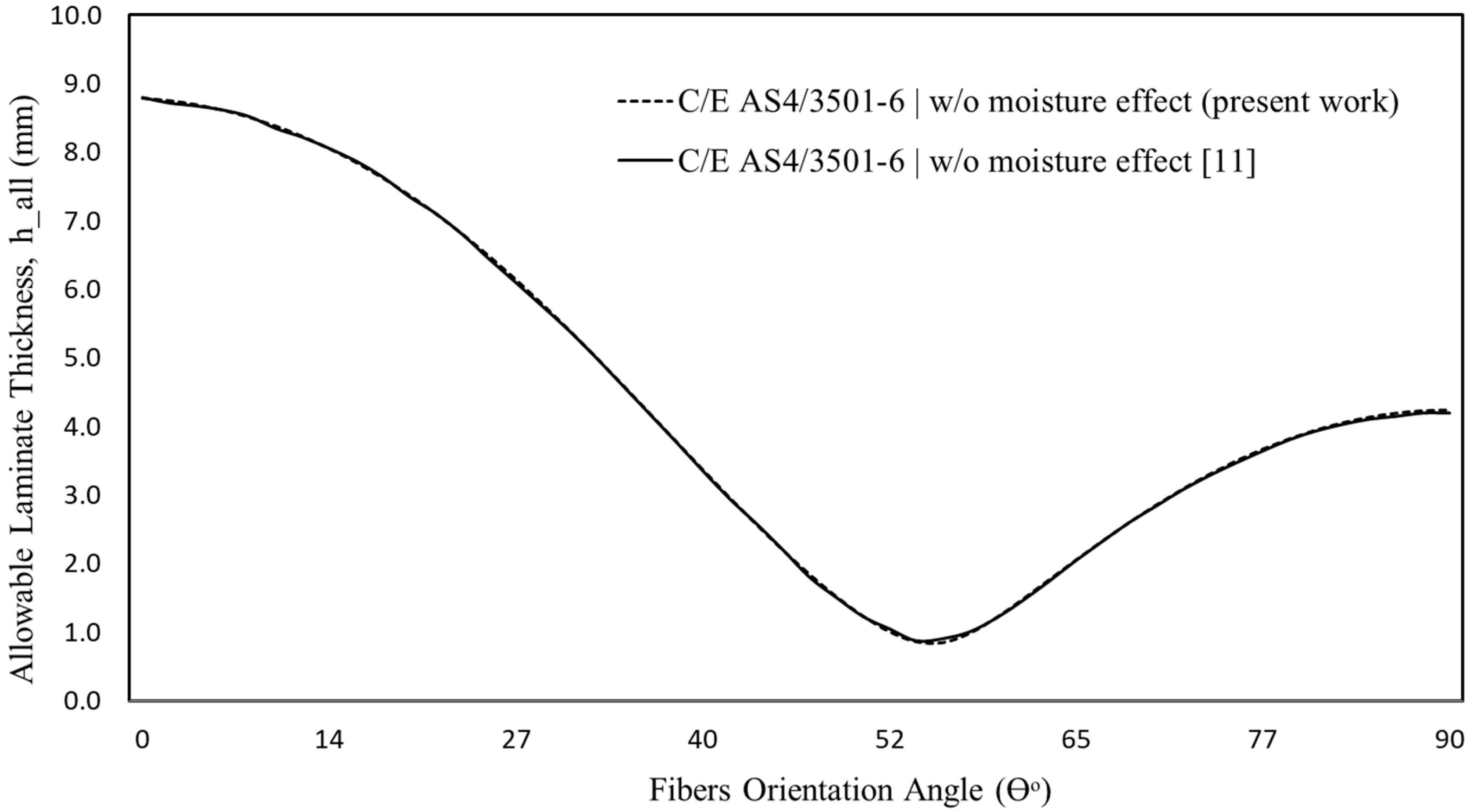
The analysis of four sizes of PV made of SST 316L, C/E AS4/3501-6 and C/E IM7/977-3 was performed. Figure 4 verifies the solution used in this study with previous work, where both studies were made on the same composite material C/E AS4/3501-6, with the same geometries and without considering the moisture effect. The same program was later on used for the material IM7/977-3 and was extended to include the moisture effect.

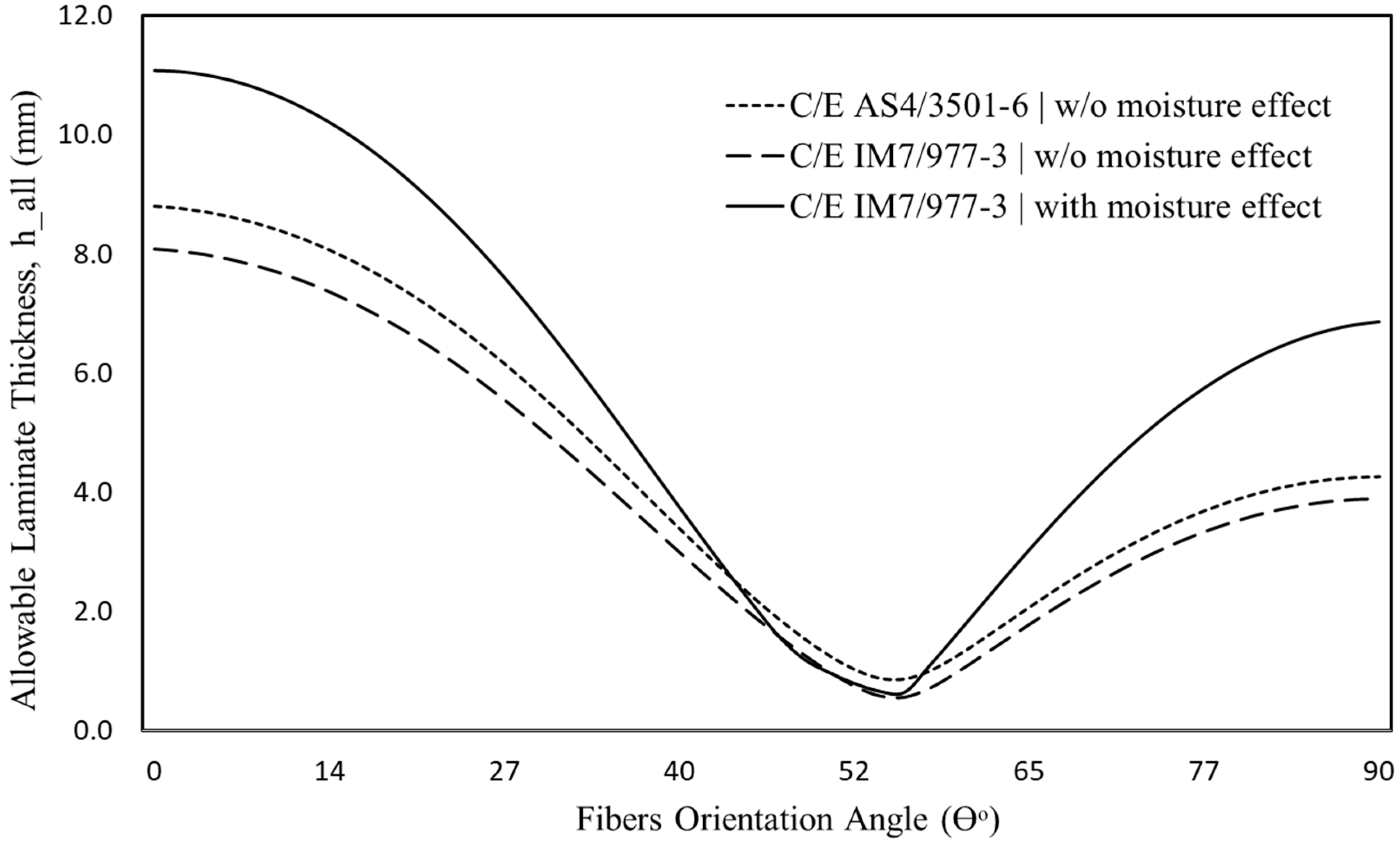
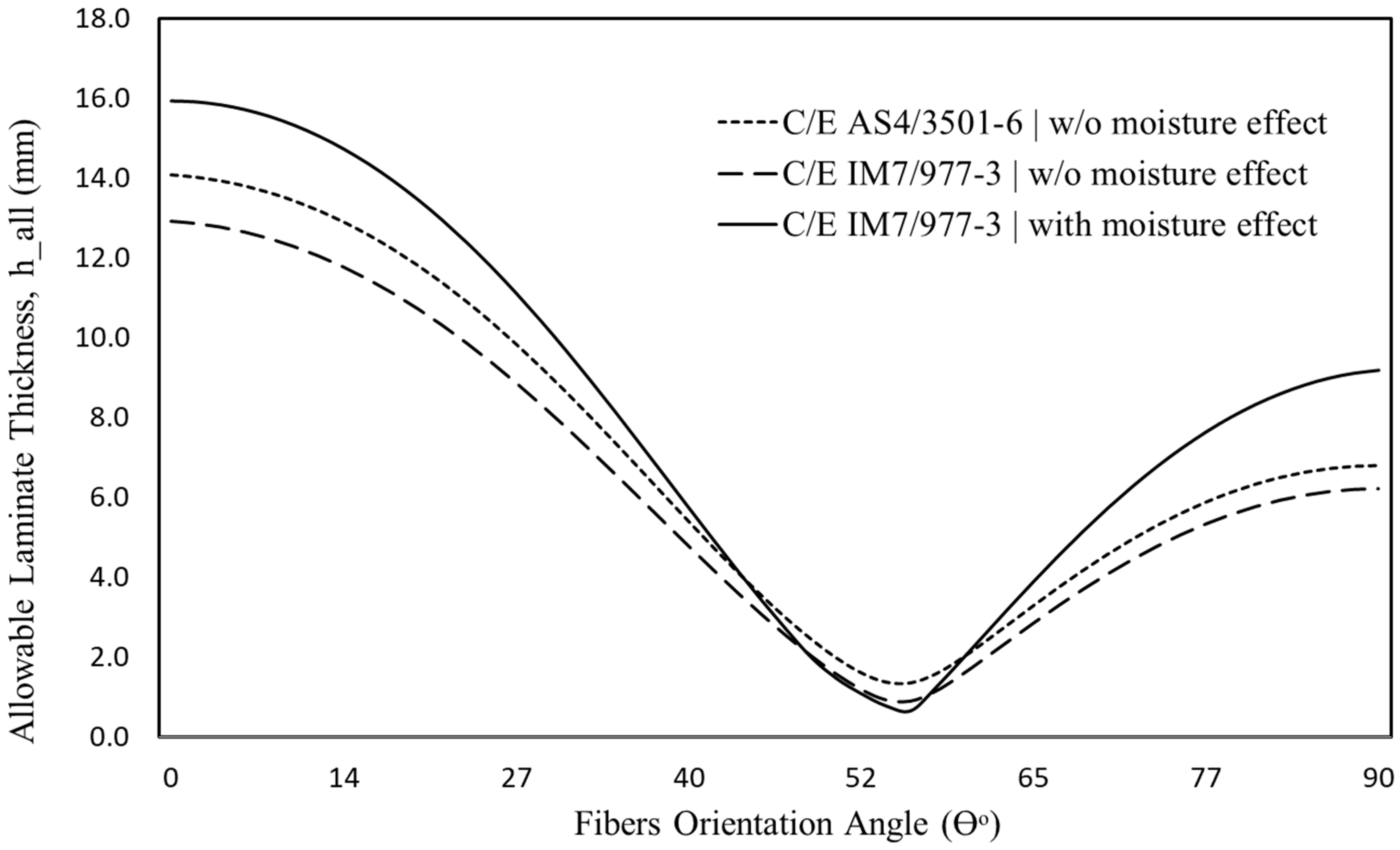
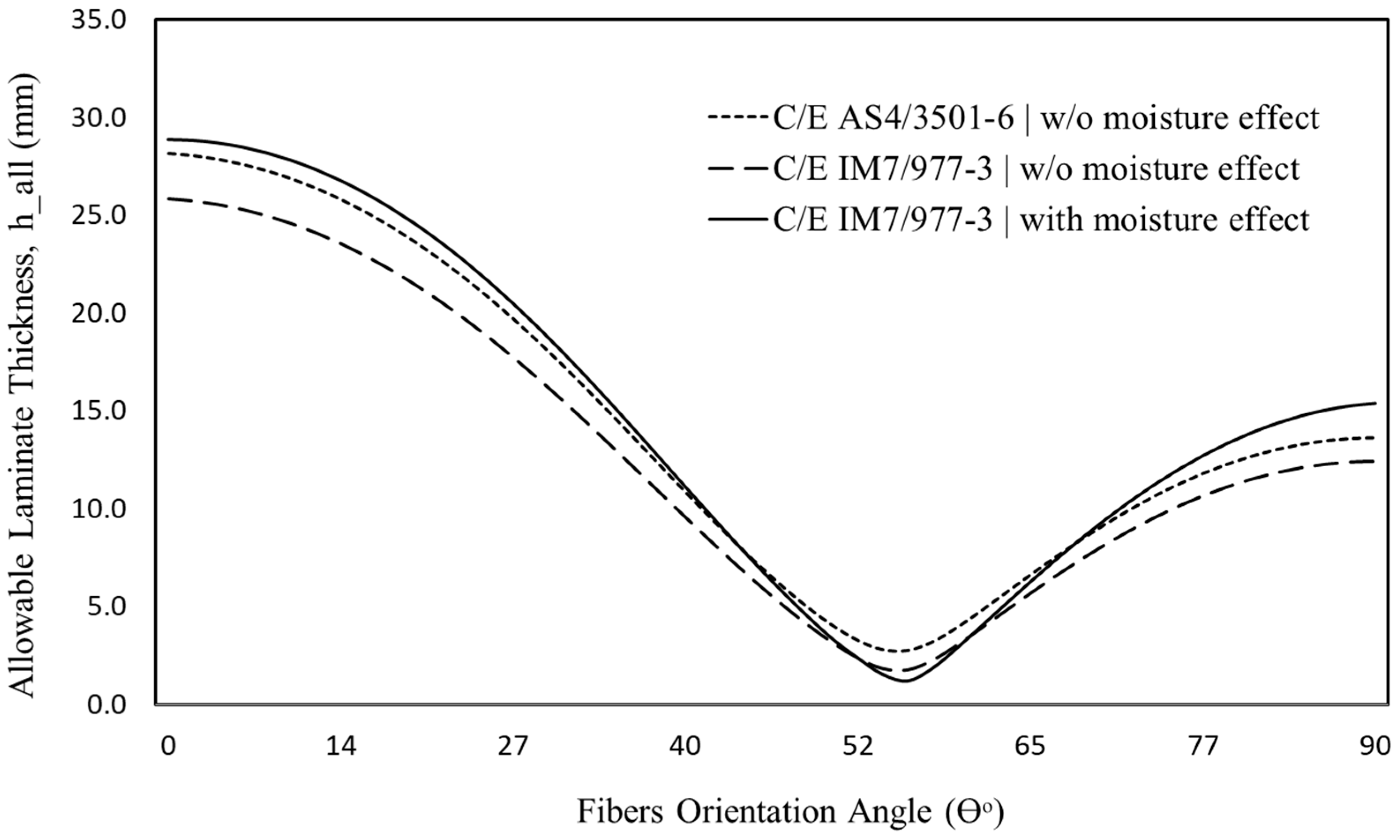
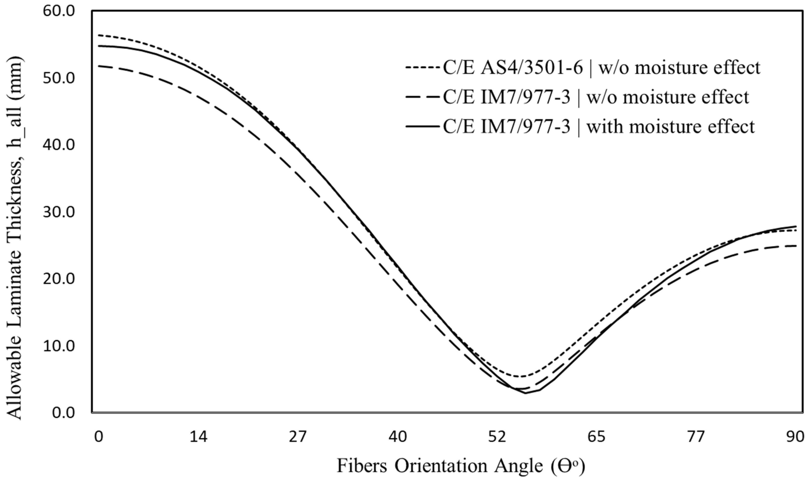
The relations between the fiber orientation angle and the allowable thickness for PV size 2.5″, 4″, 8″ and 16″ were plotted in Figure 5, Figure 6, Figure 7 and Figure 8, respectively. Each figure shows three solutions; one for C/E AS4/3501-6 PVs and two for C/E IM7/977-3 PVs, with and without the moisture effect.

The solutions shown in Figure 5, Figure 6, Figure 7 and Figure 8 for C/E AS4/3501-6 are in good agreement with the literature in terms of the general trend and the values obtained for the minimum allowable vessel thickness and fibers optimum angle [11,16]. In literature, ${\mathrm{h}}_{\mathrm{all}.\min }$ achieved for the four vessel sizes of SST 316L was 2.125, 3.401, 6.801 and 13.602 mm, and in this work it was 2.125, 3.400, 6.804 and 13.608 mm, for C/E AS4/3501-6, ${\mathrm{h}}_{\mathrm{all}.\min }$ and ${\mathsf{\theta }}_{\mathrm{opt}}$ was found in the literature as 0.847, 1.355, 2.710 and 5.419 mm, and (±55)ns, and in this work 0.847, 1.355, 2.711 and 5.421 mm and (±55.1)ns, respectively.

Figure 5, Figure 6, Figure 7 and Figure 8 also show that when C/E IM7/977-3 was used, the allowable vessel thickness for all PV sizes decreased, or the specific strength of all PV increased, which was due to the higher strength of the material (see material properties in Table 3).

The minimum allowable thicknesses achieved were 0.56, 0.90, 1.80 and 3.59 mm for the four PV sizes, and the optimum fiber angle was (±55.8)ns. This relates to a decrease of 34.1%, 33.3%, 33.6% and 33.8% in allowable thickness over C/E AS4/3501-6.

When the moisture effect was added to the composite C/E IM7/977-3, it strengthened the PV around the optimum angle and weakened it everywhere else, as can be seen in Figure 5, Figure 6, Figure 7 and Figure 8. However, in Figure 5, which corresponds to the 2.5″ size, the moisture solution did not follow the trend of other figures in strengthening around the optimum angle. This can be explained by realizing that, unlike the other two solutions, moisture loading is more affected by the size of the PV. In order to capture this relation, the decrease in the allowable thickness of composites relative to the SST 316L thickness for the three studies was determined and shown in Figure 9, using the following relation:

$$\left(1-\frac{{\mathrm{h}}_{\mathrm{i}.\mathrm{all}.\min }}{{\mathrm{h}}_{\mathrm{SST}.\mathrm{PV}}}\right)\ast 100$$

(30)

where ${\mathrm{h}}_{\mathrm{i}.\mathrm{all}.\min }$ is the minimum allowable thickness in mm, for the three composite material studies, C/E AS4/3501-6 without moisture, C/E IM7/977-3 with and without moisture. The PV allowable thickness for SST 316L is ${\mathrm{h}}_{\mathrm{SST}.\mathrm{PV}}$. When Equation (30) is applied, composites without moisture show independence of PV size, where the one with moisture shows a relatively large dependency. The ${\mathrm{h}}_{\mathrm{all}.\min }$ decrease (in mid-range) for C/E AS4/3501-6 was found as 60.15 ± 0.15%, for C/E IM7/977-3 without moisture as 73.6 ± 0.1% and for C/E IM7/977-3 with moisture as 76.05 ± 6.15%.

The SF in

Table 4. Weight, safety factor and optimum lay-up comparison for all solutions.

Size	Material	Moisture	$\mathbf{S}{\mathbf{F}}_{\mathbf{m}\mathbf{i}\mathbf{n}}$	$$\begin{gathered} {\mathbf{W}}_{\mathbf{m}\mathbf{i}\mathbf{n}} \\ \left(\mathbf{kg}\right) \end{gathered}$$	$$\begin{gathered} {\mathbf{W}}_{\mathbf{r}} \\ (\%) \end{gathered}$$	No. of Laminas	Optimum Lay-up
2.5′	SST 316L	No	2.00	1.36	-	-	-
	C/E AS4/3501-6	No	3.72	0.21	84.8	08	(±55.1)2S
	C/E IM7/977-3	No	2.85	0.10	92.3	04	(±55.8)S
	C/E IM7/977-3	Yes	2.50	0.10	92.3	04	(±54.0)S
4′	SST 316L	No	2.00	8.69	-	-	-
	C/E AS4/3501-6	No	2.33	0.82	90.6	08	(±55.1)2S
	C/E IM7/977-3	No	3.57	0.84	90.4	08	(±55.8)2S
	C/E IM7/977-3	Yes	2.41	0.41	95.2	04	(±54.0)S
8′	SST 316L	No	2.00	34.81	-	-	-
	C/E AS4/3501-6	No	3.20	3.28	90.6	16	(±55.1)4S
	C/E IM7/977-3	No	2.40	2.50	92.8	12	(±55.8)3S
	C/E IM7/977-3	Yes	1.60	1.66	95.2	08	(±54.0)2S
16′	SST 316L	No	2.00	139.23	-	-	-
	C/E AS4/3501-6	No	2.03	11.46	91.8	28	(±55.1)7S
	C/E IM7/977-3	No	2.23	08.31	94.0	20	(±55.8)5S
	C/E IM7/977-3	Yes	2.19	06.63	95.2	16	(±54.0)4S

varies between the studies due to the fact that the analysis procedure increases the thickness only in an integer number of basic laminates (increments of four laminas). This increase can best be seen in Figure 10, where the final PV thickness and the allowable thickness for all studies are compared.

When the allowable thickness for all PVs was determined, the weight achieved for all studies were found using simple geometrical relations and the material properties (Table 2 and Table 3). A comparison solution for the studied cases can be found in Table 4. The reduction in weight (${\mathrm{W}}_{\mathrm{r}}$) was determined relative to the weight of SST 316L PV and the maximum weight reductions can be found in Table 4. Figure 11 and Figure 12 show the weight reduction in relation with the fibers angle; it can be seen from the figures that for small sizes the curves are less smooth, which is expected because an increment of four laminas has a bigger impact for the smaller vessels than the larger ones.

4. Conclusions

In this work, design and failure analyses of four standard sizes of pressure vessels (SWRO PVs) were carried out in order to come up with the minimum allowable thickness of the vessel under an internal pressure loading. The PVs were made of stainless steel SST 316L and composite material C/E AS4/3501-6 and C/E IM7/977-3. The PVs were loaded by an internal pressure of 8 MPa. At first, the three materials were analyzed without considering the moisture effect, and then the moisture effect was included in another study for C/E IM7/977-3 PV. The analysis in all studies assumed a plane stress condition and was made on the cylindrical part of the PV. For SST 316L PV, the von Mises criterion was used. For the composite materials, Tsai–Wu criterion was used. A MATLAB code was developed to perform the analysis. The solutions show that using C/E AS4/3501-6 resulted in an average reduction for the PV allowable thickness by 60.18% using the optimum fibers angle (±55.1)ns, while for C/E IM7/977-3 the reduction was 73.58% using the optimum fibers angle (±55.8)ns. When the moisture effect was considered, it showed that the real values of reduction in allowable thickness were even higher (i.e., an average of 77.8% for C/E IM7/977-3 using (±54.0)ns). Also, the allowable thickness required became dependent on the size of the PV.

References

- Yan, H.G.; Liu, Z.M.; Xie, Y.J. Buckling optimization of hybrid-fiber multilayer-sandwich cylindrical shells under external lateral pressure. Compos. Sci. Technol. 1996, 56, 1349–1353. [Google Scholar]
- Katirci, N.; Parnas, L. Design of fiber-reinforced composite pressure vessels under various loading conditions. Compos. Struct. 2002, 58, 83–95. [Google Scholar]
- Krikanov, A.A. Composite pressure vessels with higher stiffness. Compos. Struct. 2000, 48, 119–127. [Google Scholar] [CrossRef]
- Chang, S.-H.; Son, D.-S. Evaluation of modeling techniques for a type III hydrogen pressure vessel (70 MPa) made of an aluminum liner and a thick carbon/epoxy composite for fuel cell vehicles. Int. J. Hydrog. Energy 2012, 37, 2353–2369. [Google Scholar]
- Wang, G.; Dar, U.-A.; Mian, H.H.; Zhang, W. Optimization of Composite Material System and Lay-up to Achieve Minimum Weight Pressure Vessel. Appl. Compos. Mater. 2013, 20, 873–889. [Google Scholar]
- Sun, C.T.; Hu, H. The equivalence of moisture and temperature in physical aging of polymeric composites. J. Compos. Mater. 2003, 37, 913–928. [Google Scholar]
- Ayoub, G.M.; Malaeb, L. Reverse osmosis technology for water treatment: State of the art review. Desalination 2011, 267, 1–8. [Google Scholar]
- Kim, Y.M.; Kim, S.J.; Kim, Y.S.; Lee, S.; Kim, I.S.; Kim, J.H. Overview of systems engineering approaches for a large-scale seawater desalination plant with a reverse osmosis network. Desalination 2009, 238, 312–332. [Google Scholar] [CrossRef]
- García-Rodríguez, L.; Peñate, B. Current trends and future prospects in the design of seawater reverse osmosis desalination technology. Desalination 2012, 284, 1–8. [Google Scholar]
- Porter, M.C. Handbook of Industrial Membrane Technology; Elsevier: Amsterdam, The Netherlands, 1989. [Google Scholar]
- El-Sayed, T.A.; El-Butch, A.M.A.; Farghaly, S.H.; Kamal, A.M. Analytical and finite element modeling of pressure vessels for seawater reverse osmosis desalination plants. Desalination 2016, 397, 126–139. [Google Scholar]
- Hanbury, W.T.; Hodgkiess, T.; Al-Bahri, Z.K. Optimum feed temperatures for seawater reverse osmosis plant operation in an MSF/SWRO hybrid plant. Desalination 2001, 138, 335–339. [Google Scholar]
- Nisbett, K.; Budynas, R.G. Shigley’s Mechanical Engineering Design; McGraw-Hill: New York, NY, USA, 2008. [Google Scholar]
- Kaw, A.K. Mechanics of Composite Materials; CRC Press: Qialadun, FL, USA, 2005. [Google Scholar]
- Ishai, O.; Isaac, M.D. Engineering Mechanics of Composite Materials; Oxford University Press: New York, NY, USA, 1994. [Google Scholar]
- Sayman, O.; Dogan, T.; Tarakcioglu, N.; Onder, A. Burst failure load of composite pressure vessels. Compos. Struct. 2009, 89, 159–166. [Google Scholar]
Figure 1.
Thin-walled PV made of stainless steel SST 316L.
Figure 2.
Thin-walled PV made of composite material.
Figure 3.
Location of plies in a laminate.
Figure 4.
Verification of analytical solution and the MATLAB program developed in the present work. The lay-up is (±θ)ns and the PV size is 63.5 mm in diameter and 400 mm in length.
Figure 5.
Variation of vessel thickness with fibers orientation angle for case 1, 2 and 3. The lay-up is (±θ)ns and the PV size is 63.5 mm in diameter and 400 mm in length.
Figure 6.
Variation of vessel thickness with fibers orientation angle for case 1, 2 and 3. The lay-up is (±θ)ns and the PV size is 101.6 mm in diameter and 1000 mm in length.
Figure 7.
Variation of vessel thickness with fibers orientation angle for case 1, 2 and 3. The lay-up is (±θ)ns and the PV size is 203.3 mm in diameter and 1000 mm in length.
Figure 8.
Variation of vessel thickness with fibers orientation angle for case 1, 2 and 3. The lay-up is (±θ)ns and the PV size is 406.6 mm in diameter and 1000 mm in length.
Figure 9.
The reduction of minimum allowable thickness for composite PVs relative to SST 316L PV. The figure shows the dependency between the PV size and the inclusion of moisture effects.
Figure 10.
The allowable PV thicknesses and the composites final PV thicknesses after approximating to an integer number of basic laminates.
Figure 11.
The weight reduction of 2.5″ and 4″ PVs made of IM7/977-3 compared to ones made of SST 316L for different fiber angles.
Figure 12.
The weight reduction of 8″ and 16″ PVs made of IM7/977-3 compared to ones made of SST 316L for different fiber angles.