Experimental Validation of a Direct Fiber Model for Orientation Prediction


Polymer Engineering Center (PEC), University of Wisconsin-Madison, 1513 University Ave, Madison, WI 53706, USA
*
Author to whom correspondence should be addressed.
J. Compos. Sci. 2020, 4(2), 59; https://0-doi-org.brum.beds.ac.uk/10.3390/jcs4020059
Submission received: 24 April 2020
/
Revised: 16 May 2020
/
Accepted: 19 May 2020
/
Published: 25 May 2020
(This article belongs to the Special Issue Discontinuous Fiber Composites, Volume II)
Abstract
:Predicting the fiber orientation of reinforced molded components is required to improve their performance and safety. Continuum-based models for fiber orientation are computationally very efficient; however, they lack in a linked theory between fiber attrition, fiber–matrix separation and fiber alignment. This work, therefore, employs a particle level simulation which was used to simulate the fiber orientation evolution within a sliding plate rheometer. In the model, each fiber is accounted for and represented as a chain of linked rigid segments. Fibers experience hydrodynamic forces, elastic forces, and interaction forces. To validate this fundamental modeling approach, injection and compression molded reinforced polypropylene samples were subjected to a simple shear flow using a sliding plate rheometer. Microcomputed tomography was used to measure the orientation tensor up to 60 shear strain units. The fully characterized microstructure at zero shear strain was used to reproduce the initial conditions in the particle level simulation. Fibers were placed in a periodic boundary cell, and an idealized simple shear flow field was applied. The model showed a faster orientation evolution at the start of the shearing process. However, agreement with the steady-state aligned orientation for compression molded samples was found.
1. Introduction
Over the past decade, the use of long fiber-reinforced thermoplastics (LFTs) has gained wide acceptance in the automotive industry in order to meet the increasingly tightened corporate average fuel efficiency standards [1,2]. As more efficient engines and electric powertrains will not carry the whole load, the automotive industry is pressured into finding alternative solutions. One of those solutions has been light weighting car components by retrofitting existing structures made out of steel [3,4,5,6,7]. LFTs are being considered as a substitute because they show high performance in terms of mechanical properties, are lightweight, noncorrosive, and can be tailored to satisfy performance requirements [3,5,6,8,9].
Although the mechanical advantages of LFTs are widely reported in literature, the uncertainty remains being able to accurately model this heterogenous material class. It has been shown by numerous researchers that LFTs’ mechanical performance and dimensional stability are a direct function of their microstructure, and therefore depend on fiber orientation (FO), fiber length (FL), and fiber concentration (FC) [7]. Parts are stronger in the direction of the fiber alignment and if fiber length and volume fraction (φ) are increased [10]. Being able to accurately predict the microstructure of molded components is a key factor in the automotive industry, not only for design calculations and a successful process, but also for an optimized part’s performance and for guaranteeing parts are safely introduced into vehicles.
Continuum-based models for fiber orientation [11,12,13,14], length distribution [15,16], and fiber content prediction [17,18,19] have been developed in the last decades. These models employ a probabilistic approach to obtain the fiber configuration evolution during processing which is based on the input parameters, such as fiber characteristics and flow conditions. These models are computationally very efficient and have been implemented into commercial software. However, they can only describe the mechanism of fiber–matrix separation, fiber-attrition, and fiber alignment individually. They lack a linked theory between the three mechanisms and their interdependency [7]. Additionally, these models require experimentally determined fitting parameters. Conducting these experiments is costly, lengthy, and their provided information is limited.
Particle level simulations (PLS) have been used in the past for microstructure predictions in the plastics industry to learn about the real mechanisms present in processing discontinuous fibers [20,21,22]. PLS provide a fundamental modeling approach, as they solve the forces and moments acting on individual fibers during processing by accounting for the complex interactions of fibers and matrix. Compared to continuum models, the state and motion of fibers are not described as averaged and homogenized properties, but rather by solving the governing equations of each fiber explicitly. Hydrodynamic forces, fiber flexibility, excluded volume forces, fiber–fiber, and fiber–wall contacts are taken into account, leading to more accurate simulation results [7,23]. Additionally, PLS can be used to determine the fitting parameters of continuum models numerically. This has advantages as all parameters can be accurately controlled, detailed information is always available, and simulations are relatively inexpensive to perform.
PLS of semi-concentrated to concentrated fiber suspensions must address two central problems: First, the formulation of the equation of motion for individual fibers. Second, the particle–particle interactions, which can affect the flow behavior. To do this, various approaches have been taken in the past. Yamane et al. [24] represented fibers a rigid rods and calculated motion based on Jeffery’s theory. They considered only short range interactions and modeled them with lubrication theory. Fan et al. [20] extended Yamane’s work with rigid fibers. They accounted for long range interactions by employing a slender body approximation. Fan and co-workers later used a chain of beads joined with connectors to model flexible fibers, improving their viscosity predictions [25]. Schmid et al. [26] used PLS to study fiber flocculation. They modeled fibers as chains of rigid rods interconnected with hinges. Rods could rotate and twist about the hinges, replicating fiber bending and twisting deformations. They modeled interactions by considering repulsive forces acting normal to fiber surfaces to represent the fiber’s excluded volume, and frictional fiber forces which prevented fibers from sliding over one another.
The objective of this work is to generate reliable FO evolution data in a well-defined simple shear flow to aid in the validation and development of our PLS. Simple shear was chosen as it is one of the fundamental flow conditions present in most polymer processes, such as injection molding (IM). This allows us to directly correlate the rate of deformation with the filler’s behavior. IM and compression molded (CM) glass fiber-reinforced polypropylene samples were sheared in a Sliding Plate Rheometer (SPR) following Cieslinski et al. [27]. As has been shown by the same author, CM has no control over the planar orientation of the fibers, and is therefore not a suitable sample preparation method. This work will present a CM technique which ensures a controlled and repeatable initial FO for shear experiments. Results from both simulation and experiment are presented in this work.
2. Direct Fiber Model
The direct fiber or mechanistic model, used in this work, was developed at the Polymer Engineering Center, University of Wisconsin-Madison, USA, and is based on Schmid et al. [26]. Every single fiber is discretized as a chain of rigid elements with circular cross sections of diameter D, interconnected with spherical joints. The joints elastically couple the segments of a fiber as shown in Figure 1.
In the model, inertial effects are neglected due to the low Reynolds numbers (Re) that result from the high viscosity of the polymer matrix. It has been shown experimentally by Hoffman [28] and Barnes [29] that inertial effects become important at Re ≥ 10−3. In our work, the Re was calculated to be in a range of 10−9–10−4. Long-range hydrodynamic interactions are neglected as well due to the fluid’s high viscosity [30]. Additionally, extensional and torsional deformations are neglected as fluid forces are not sufficiently high to cause fiber stretching or torsional deformation. Only bending deformation is included in the model. Brownian motion can be neglected as the Peclet number (Pe) is well above 103 and at this point Brownian interactions are disrupted by hydrodynamic forces [31]. Buoyant effects are neglected in the model as well [7,32]. The presence of fillers in any suspension modifies the flow field, especially in the semi-diluted and more concentrated regimes. However, the coupling between particle and fluid is not considered in the present formulation due to its high computational cost [32].
The force calculation for a segment includes the drag force , the interaction force with an adjacent segment , and intra-fiber forces exerted by internal connection loads at the nodes. The translation equation of motion is
The rotational equation of motion is equally derived and includes elastic recovery terms and a hydrodynamic torque
where describes the shortest distance vector between two segments. Some of these quantities are presented in Figure 2. A fiber divided into more than one element requires an extra constraint that enforces connectivity between the different elements
Hydrodynamic effects are approximated by modeling each fiber segment as a chain of beads. The hydrodynamic force is the sum of forces experienced by the beads and is described as
is given by Stokes law, where describes the number of beads, the bead radius, the polymer matrix viscosity, the surrounding fluid velocity, and the velocity of the bead ().
is then be written as
Due to the fluid’s vorticity each bead is also subjected to a hydrodynamic torque
where the hydrodynamic contribution of bead is
is the vorticity of the surrounding fluid and is the angular velocity of the bead . Substituting the expression of and the expression of into the fluid’s vorticity we can write
The fiber–fiber interaction force is decomposed in a normal force and a tangential force
describes the friction between the segments and starts acting when the distance between adjacent fibers, , is below a defined threshold . is an excluded volume force which is implemented as a discrete penalty method [7,32,33]. usually has a function of the following type [26,34,35],
where is the shortest distance between rod and rod , the fiber diameter, and is the vector along the closest distance between the rods. and are parameters for which different values have been presented in the literature [26,34]. In this work, has been chosen empirically to avoid the overlapping of fibers. value of 1000 N was the minimum constant value at which penetrations cease to occur in the simulation [32]. was set to 2.
The friction force between segment and is computed as
is the Coulomb coefficient between fibers, is the vector of the relative velocity between elements.
Bending of a fiber was approximated by using elastic beam theory
with as the bending moment, as the angle between segments, and as the segment length.
A linear system of equations was assembled and solved to find the velocities and connective forces in each fiber. These velocities were integrated over time using an explicit Euler scheme to determine the fiber trajectory during the simulation [7].
3. Test Setup and Experimental Validation
3.1. Sample Preparation
The fiber suspension used in this work was a 10 and 20 wt % glass fiber in a polypropylene (PP) matrix. The 20 wt % (STAMAX PPGF20) was commercially available and provided by SABICTM. The material was supplied in the form of coated pellets with a nominal length of 15 mm, which also represents the initial and uniform length of the glass fibers. The used E-glass fibers (ρ = 2.55 g/cm3) are chemically coupled to the PP matrix (ρ = 0.91 g/cm3). The fiber diameter was measured to be 19 ± 1 μm using an optical microscope. The 10 wt % was achieved by mixing higher FCs with neat PP (SABICTM PP579S) in a cement mixer. The neat PP is identic to the matrix material for the commercial available STAMAX pellets. The matrix was considered as a generalized Newtonian fluid under the test conditions presented. The authors of [27,36] showed that the presence of polymer matrix eliminates any concerns regarding fiber sedimentation due to gravity.
Two separate processes were used to prepare samples that were tested in the SPR. The first method combined extrusion to disperse fibers and compression molding to form proper sample dimensions. The second approach used IM to produce plates.
The first sample preparation method used an Extrudex Kunstoffmaschinen single-screw extruder to process the pultruded material. The 45 mm 30 L/D extruder was equipped with a gradually tapering screw and fitted with a 3 mm die. The temperature zones of the extruder were set to 210, 210, 220, 220, 230, 230, and 230 °C and the die temperature was set to 230 °C. The composite was extruded at 5 rpm. Due to the low processing speed, most of the initial FL was maintained in the extruded strand (LN = 6.7 mm, LW = 11.4 mm). Computational time for the mechanistic model simulation is geometrically proportional to the maximum detected FL. To reduce computation, the strands were pelletized to 3.2 mm. Initial compression molding trials showed that manual alignment of pellets in the mold did not yield a repeatable initial FO, because pellets could move easily and rotate. Therefore, pellets were re-extruded and strands were cut to fit mold dimensions. The mold geometry was a rectangular prism (14 mm × 14 mm × 2.1 mm). Analysis of the re-extruded strands showed a LN of 0.83 mm and LW of 1.53 mm. The mold was coated and placed on a heating plate to cause partial melting of the aligned strands. This facilitated space reduction between irregular shaped strands. The plate was extracted, flipped 180°, and re-molten to remove trapped air bubbles between strands. Failure to remove caught air bubbles would alter matrix rheology. Plates were compression molded at 210 °C and a load of 1000 lbs. Final fiber properties are summarized in Table 1.
The second sample preparation procedure involved IM a simple plate geometry (102 × 305 × 2.85 mm3). The cavity was filled through a 20 mm edge-gate with the same thickness as the plate and was fed through a 17 mm full-round runner. Parts were molded on a 130 ton Supermac Machinery SM-130 IM machine. The melt temperature was set to 250 °C, and back and holding pressure to 5 and 300 bar, respectively. Injection and holding time were set to 2 and 22 s, respectively. A full microstructure analysis was conducted. Fiber properties are summarized in Table 1. Samples for the SPR were only extracted from regions which showed a clear developed shell–core structure and identic FCs [4].
For both sample preparation methods, the SPR sample sizes were calculated by adding 20 mm to the stroke applied to be able to extract pure shear samples for FO analysis.
3.2. Sliding Plate Rheometer
FO evolution data was obtained in a SPR by shearing samples in a controlled simple shear flow (Figure 3). The rheometer was based on the design of [37]. The SPR was contained in a convection oven and the rectilinear plate displacement was generated by an Interlaken 3300 universal testing instrument. The rheometer had an effective surface of 100 × 300 mm2 and a maximum stroke of 120 mm. The SPR gap thickness could be altered. However, it was chosen to be 2 mm, as this work yields to aid in the understanding of how fibers flow and orient themselves during the IM process. Typically, IM parts show a thickness of 2 mm. The maximum possible displacement and the chosen gap size, limited the deformation that could be imposed on the sample to a shear strain of 60. Both, shear rate and shear strain, were programmable through the Wintest® Software (Bose Corporation, Eden Prairie, MN, USA).
The experimental procedure was based on the SPR experiment conducted by [27]. The rheometer was heated to 260 °C for 2 h prior to sample loading. Upon loading, the test specimen was rotated 90° with respect to the extrusion/filling direction, effectively swapping the a11 and the a22 components of the orientation tensor. This allowed for a low alignment in the shearing direction, so a larger change in orientation could be observed. The sample was secured between the rheometer plates and allowed to melt evenly before the plates were tightened to a final gap of 2 mm (=initial condition). As the initial thickness of the test specimen was larger than the final gap thickness, samples were slightly compressed when tightening the plates to guarantee full contact. After an additional 10 min of heating, the sample was sheared at a rate of 1 s−1. Forced convection was used to cool the sample to preserve its shape and FO for further analysis. Five repetitions per testing condition were used to ensure accuracy and repeatability of results.
3.3. Measurement of Fiber Microstructure
A fully characterized microstructure was required to accurately reproduce the initial conditions in the direct fiber simulation (Figure 4). FO was determined by using the X-ray microcomputed tomography (μCT) approach. A sample of dimensions 10 × 10 × 2 mm3 was loaded into a sample holder and then placed on a rotating platform. The X-rays penetrated the sample and were absorbed differently depending on the configuration of the sample’s constituents. The detector recorded the attenuated X-rays as radiographs at incremental angles during the rotation of the sample to achieve a full scan of the sample. After completion of the 3D reconstruction, the μCT data set was processed with the VG StudioMAX (Volume Graphics) software to quantify the FO distribution using the structure tensor approach [4,38,39]. Samples were scanned with an industrial μCT system (Metrotom 800, Carl Zeiss AG, Oberkochen, Germany). Throughout the reported studies, the voltage was set to 80 V, the current to 100 A, the integration time to 1000 ms, the gain to 8, the number of projections to 2200, and the voxel size was set to 5 μm.
FC was quantified with VG StudioMAX as well. The μCT data set was converted into a stack of 2D cross-sectional images aligned normal to the thickness direction. The grayscale images were transformed into binary images by thresholding, which separated the image into black (matrix) and white (fibers) pixels. Subsequently, the fiber volume fraction through the thickness was calculated [4].
The FL measurement technique presented in [40] was employed in this work. This technique consists of fiber dispersion and a fully automated image processing algorithm to quantify the fiber length distribution (FLD). It has been shown in [41] that downsampling methods yield to a preferentially capture of long fibers, and thus skew the real FLD. In this work, a correction was therefore applied to all results as published by [41].
4. Direct Fiber Simulation
4.1. Simulation
To set up a simulation that matches the SPR experiment, a number of fibers matching the experimental volume fraction was placed inside a shear cell. To guarantee a constant fiber volume fraction, Lees–Edwards periodic boundaries [42] were assigned to the cell faces perpendicular to the shearing direction (Figure 5). Mechanical properties were assigned to the fibers while rheological properties were assigned to the matrix. A simple shear flow field was applied to the matrix phase which translates into the hydrodynamic force term in the force balance calculation explained in Section 2.
4.2. Simulation Setup
In order to obtain reliable rheological information from discontinuous fiber composites, accurate and repeatable initial conditions are needed [27]. To create the initial cluster of fibers for the simulation, the microstructure of the experimental samples was carefully characterized. The experimental values of orientation (aij) and fiber density (vol %) were reproduced by discretizing each through-thickness profile into a set number of layers as shown in Figure 6. For each layer the average orientation tensor components were used to reconstruct the fiber orientation state by using a Fourier Series expansion. It is worth noticing that as the thickness of the individual layers is decreased, to obtain better resolution, the target off-plane orientation becomes harder to achieve.
The average FLs (LN, LW) were assigned as a global length distribution to the complete cluster of fibers. This distribution was obtained by fitting a Weibull probability distribution function to the experimental length measurement. The result was a heterogeneous cluster of fibers closely resembling the experimental condition (Figure 7). Prior to imposing the shear flow, a short simulation was conducted with no velocity field and only interaction forces present. This was applied as a relaxation step, so fibers are not overlapping or in extreme proximity at the start of the shearing simulation. This step does not modify the initial orientation state in a significant way.
A simple shear flow with a rate of deformation of 1 s−1 was applied to the shear cell. The viscosity was set to 110 Pas using the properties of the neat PP. The dimension of the cell is dictated by the SPR gap in Z direction of 2 mm. To allow free rotation, the dimension in X and Y were set to 1.1 times the length of the longest fiber. The cluster properties corresponding to both sample preparation methods are listed in Table 2.
The simulation time was set to 60 s to obtain a total strain of 60. Cell walls parallel to the YZ plane have a periodic boundary condition. A tight array of fixed fibers is placed on the upper and lower boundaries to represent the SPR walls. The additional input parameters for the simulation are listed in Table 3. The simulation results were the coordinates of each fiber at every time step. With this information orientation tensors were calculated as a function of time and strain.
5. Results and Discussion
5.1. Injection Molded Samples
IM provides a repeatable flow history that will yield to FO that is consistent among multiple samples [4,27]. The global diagonal components of the orientation tensor at zero shear strain are shown in Figure 8. The common core–shell structure associated with molded composites can be seen. The core layer consists of fibers predominantly aligned in cross-flow direction (a22), while fibers in the shell are oriented along the flow direction (a11) due to the fountain flow effect. The orientation in thickness direction a33 is uniform and generally low with average values less than 0.06 [4].
The average orientation tensor as a function of shear strain is shown in Figure 9. For both simulation and experiment fibers gradually align in the flow direction over 60 shear strain units. The general trend of a11 for the experimental data begins at 0.53 and evolves to a value of 0.63. In contrast, the simulation starts at a value for a11 at 0.60 and evolves to a value of 0.74. The computational initial condition differs from the experimental one due to two main reasons: First, the complex core–shell structure present in the IM sample is difficult to discretize (Figure 8). There will be a loss of accuracy by averaging the orientation data into seven layers. Second, the FL of the experimental sample is very high which increases the shear cell size and therefore computational time. Therefore, the FL was truncated in the simulation. As the initial conditions were not accurately reproduced, a different rate of orientation evolution was obtained in the PLS. However, experiment and simulation still show similarities in their behavior. Both show a slight drop in a11 before fibers start aligning in shearing direction. This drop is less pronounced in the PLS, as fibers start off with a higher a11 alignment. An initial decrease in a11 was also found in [27]. In their work, this phenomenon was explained as follows. Fibers oriented slightly out of the 1–2 plane need to flip first to become oriented in flow direction, leading to an increase in a13, thus a decrease in a11. This increase in a13 could be seen in the experimental data. Depending on the initial value of a13, the alignment in flow direction is different. If a13 is positive, the fiber will continue to align in flow direction. However, an initial negative a13 orientation would require the fiber to flip before becoming aligned in flow direction. It is expected that a fiber with a negative a13 would take longer to align in flow direction [27]. A slight initial decrease in a11 was also reported by [44]. The used SPR was limited to 60 strain units and a steady state response associated with fiber suspensions could not be obtained.
The simulation results for a11 through thickness were smoothed and plotted for different strains in Figure 10. Under a constant shear, the complex heterogeneous orientation profile transitions into a more homogeneous profile.
5.2. Compression Molded Samples
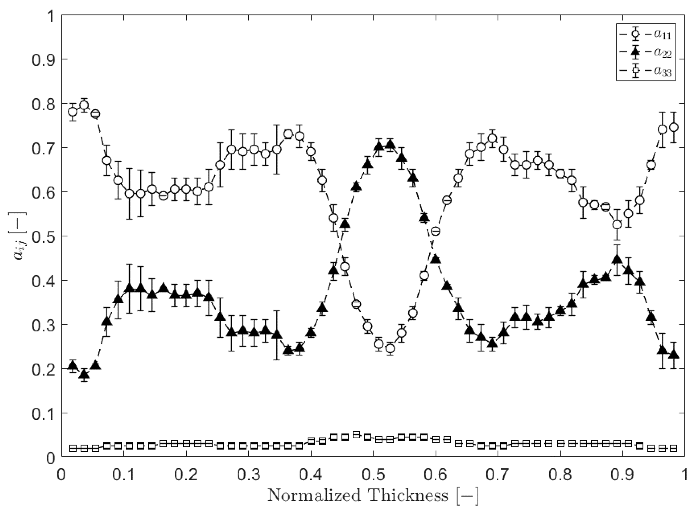
It has been shown that IM samples provide a repeatable initial FO; however, IM specimens show a complex core–shell structure, which is difficult to reproduce computationally (Figure 8). In addition, samples showed a high alignment in shearing direction at zero strain; therefore, only a low further alignment of a11 could be observed (Figure 9). CM samples with a controlled FL, FC, homogenous structure, and with a low a11 alignment were consequently manufactured to accurately reproduce the initial conditions (Figure 6).
The average orientation through sample thickness as a function of shear strain is shown in Figure 11. Initial conditions could be accurately reproduced computationally and fit the experimental data. The standard deviation for experimental values at zero strain is low, which demonstrates a repeatable initial FO, validating the CM sample preparation method.
The a11 component starts at 0.36 and transitions to a steady-state value of approximately 0.7 for both the experiment and the PLS. A steady state is reached at a total strain of 50. A slight initial drop in a11 could be seen in the experimental data, but was not present for the PLS. The simulation shows faster orientation evolution than the experiment. This phenomenon has also been reported in literature [45,46] for other diffusion models. It has been established that Jeffrey’s hydrodynamic model and Folgar–Tucker’s model predict a faster transient orientation rate when compared to related experiments [46]. Therefore, recent models have been developed with slow fiber orientation kinetics. Wang et al. [12] introduced the reduced strain closure model. This model employs a scalar factor to slow the orientation dynamics. Results still showed a quicker initial rise of flow-direction orientation, but achieved nearly the same steady state orientation as obtained with experiments [45]. In an attempt to slow the orientation kinetics predicted, Phelps et al. [13] derived the anisotropic rotary diffusion model.
The distortion of the flow field due to the presence of particles gives rise to the particular rheology of suspensions. As the aspect ratio () of the particles increases, this effect becomes dependent on the orientation state, as described by Dinh et al. [47]. Lindstrom et al. [34] conducted a PLS with individual fibers in simple shear flow. They observed orbit periods were overestimated when not including two-way coupling. They concluded that particle–fluid interaction is essential to the fiber’s dynamic behavior in shear flow. In that regard, neglecting the two-way coupling between the fiber orientation state and the underlying flow field in a PLS, can be a considerable source of error. However, various authors have shown that including two-way coupling has marginal effect on the orientation state for flow in common geometries. Mezi et al. [48] pointed out that accounting for the coupling effect had little impact on the fiber orientation distribution for the fluid flow in a planar channel, while having a considerable effect in the pressure drop. They also observed coupling increased the size of corner vortex in a contraction geometry. This last effect was also noted by VerWeyst et al. [49], who observed moderate impact of coupling on the fiber orientation in a center-gated disk. They showed effects of coupling decayed rapidly with increasing distance from the center of the disk. The difficulty with these approaches lies in the large computational domain required to resolve both the spatial and orientation domains. With PLS the computational cost increases rapidly as the two-way coupling must be calculated for each fiber.
In a PLS study for SFTs under simple shear, Kugler et al. [50] also observed a faster alignment in the simulation with respect to the experimental data. They suggested a reduced shear strain to correct for the lack of two-way coupling. Similarly, in an experimental study of fiber attrition employing a Couette rheometer, Moritzer et al. [51] use the scale factor ) to account for the reduced rate of deformations experienced by fibers in the suspension.
Published work indicates that the coupling effect might have a greater impact on the fiber orientation in the dynamic portion of the orientation evolution, and that aspect ratio and volume fraction are scaling factors of such effect. A PLS study to determine quantitatively the impact of coupling under simple shear flow remains to be done; one that compares the predicted orientation to the complete microstructural data determined experimentally.
The a13 and a12 components of orientation are shown in Figure 12. In both prediction and experiment a13 and a12 show close agreement with the final steady state value. The measured a13 component shows small oscillations. This behavior indicates some fibers orbit in the plane of shear. The predicted a13 component also shows these orbits, however, with a shorter period. The initial measured a13 component has a negative value of −6 × 10⁻⁴, while the computational cluster started with a very small, yet positive, value of 6 × 10⁻⁵. Literature suggests that the initial value of a13 impacts whether components of orientation evolve monotonically to a steady state or present an overshoot and/or undershoot prior to reaching a steady state [52]. The fact that the initial computational cluster differed from the experimental one in this aspect, is a factor in why the a11 component oriented directly to steady state in the simulation, while the experimental a11 did show a slight undershoot (Figure 11). It can be seen that a12, for the simulation, increases continuously with shear strain. As fibers oriented in the 1–2 plane orient themselves in 1, the value of a12 should approach zero.
The mentioned faster orientation kinetics in the PLS are also shown in Figure 13. Compared to the initial orientation, the experimental core–shell structure is largely unchanged at 12.5 strain units. At the same applied strain, the simulation already shows a large transition to a rather homogenous structure. At 60 strain units, the core–shell structure disappears, a homogeneous profile is reached and a good match between experiment and the PLS was observed. It is assumed that shearing beyond 60 strain units would lead to a steady state FO through thickness [27]. The smoothed computational a11 evolution as a function of shear strain is shown Figure 14. With an increase in shear strain, the heterogeneous orientation profile transitions into a homogeneous steady state. The most significant change in orientation occurs in the core of the sample. The rate of change slows down as the orientation approaches steady state.
With the proposed CM technique, it was possible to manufacture samples with low alignment in shearing direction, which allowed a larger orientation transition. Higher alignment and faster orientation evolution was observed for the CM samples when compared to the IM ones. The faster alignment can be attributed to the lower FL of the CM samples. The long fibers present in the IM samples require more energy to rotate and also hinder the motion of adjacent fibers.
6. Conclusions and Outlook
A PLS was used to simulate the FO evolution of glass fiber-reinforced PP plates sheared in a SPR. The PLS results showed a faster orientation evolution at the beginning of the shearing process compared to the experimental data. However, an agreement with the final orientation state was observed for the CM plates after fine-tuning the initial condition discretization method. In the experiment, an early decrease in a11 was observed for IM and CM samples. The same behavior has been reported in literature by [27]. However, the author used shorter fibers compared to the FL in this work. It appears that this phenomenon is more easily observed with longer fibers due to a slower rate of FO.
A reliable sample preparation method for suspension rheology was developed. Repeatable and controlled initial orientation can be achieved through the presented CM technique. Even though it has been shown in [27] that CM samples do not exhibit repeatable orientation evolution data during the startup of simple shear flow in a SPR, the CM technique employed in this work differs significantly by manually depositing individual and aligned strands.
As the dynamics of fiber suspensions are not yet well captured by the PLS, future work will focus on implementing the effect of fiber fluid coupling and studying its impact under different combinations of the dimensionless number .
Author Contributions
S.A.S. and A.B.S. conceived and designed the experiments. S.A.S. was responsible for performing the experimental studies and the microstructure analysis. A.B.S. performed the simulations. S.A.S. and A.B.S. analyzed the data and wrote the paper. T.O. supervised the project and was involved in all stages of the research. All authors have read and agreed to the published version of the manuscript.
Funding
This research was supported by the National Science Foundation under Grant No. 1633967.
Acknowledgments
The authors would like to thank SABIC® for their ongoing support and collaboration with our research group and their material supply. Additionally, we would also like to thank our colleagues from the Polymer Engineering Center who provided insight and expertise that greatly assisted the research.
Conflicts of Interest
The authors declare no conflicts of interest.
References
- NHTSA. Corporate Average Fuel Economy (CAFE) Standards; NHTSA: Washington, DC, USA, 2020. [Google Scholar]
- Ning, H.; Lu, N.; Hassen, A.A.; Chawla, K.; Selim, M.; Pillay, S. A review of Long fibre thermoplastic (LFT) composites. Int. Mater. Rev. 2019, 65, 164–188. [Google Scholar] [CrossRef]
- Jain, R.; Lee, L. Fiber Reinforced Polymer (FRP). Composites for Infrastructure Applications; Springer: Berlin/Heidelberg, Germany, 2012. [Google Scholar]
- Goris, S. Characterization of the Process-Induced Fiber Configuration of Long Glass Fiber-Reinforced Thermoplastics. Ph.D. Thesis, University of Wisconsin-Madison, Madison, WI, USA, 2017. [Google Scholar]
- Thomason, J.L. The influence of fibre length and concentration on the properties of glass fibre reinforced polypropylene. 6. the properties of injection moulded long fibre PP at high fibre content. Compos. Part A Appl. Sci. Manuf. 2005, 36, 995–1003. [Google Scholar] [CrossRef] [Green Version]
- Nghiep Nguyen, B.; Kunc, V. An elastic-plastic damage model for long-fiber thermoplastics. Int. J. Damage Mech. 2010, 19, 691–725. [Google Scholar] [CrossRef]
- Osswald, T.; Ghandi, U.; Goris, S. Discontinous Fiber Reinforced Composites, 1st ed.; Carl-Hanser Verlag: Munich, Germany, 2020. [Google Scholar]
- Zhang, G.; Thompson, M.R. Reduced fibre breakage in a glass-fibre reinforced thermoplastic through foaming. Compos. Sci. Technol. 2005, 65, 2240–2249. [Google Scholar] [CrossRef]
- Wang, J.; Geng, C.; Luo, F.; Liu, Y.; Wang, K.; Fu, Q.; He, B. Shear induced fiber orientation, fiber breakage and matrix molecular orientation in long glass fiber reinforced polypropylene composites. Mater. Sci. Eng. A 2011, 528, 3169–3176. [Google Scholar] [CrossRef]
- Fu, S.Y.; Hu, X.; Yue, C.Y. Effects of fiber length and orientation distributions on the mechanical properties of short-fiber-reinforced polymers: A Review. Int. J. Mater. Res. 1999, 5, 74–83. [Google Scholar] [CrossRef] [Green Version]
- Advani, S.G.; Tucker, C.L. The Use of Tensors to Describe and Predict Fiber Orientation in Short Fiber Composites. J. Rheol. 1987, 31, 751–784. [Google Scholar] [CrossRef]
- Wang, J.; O’Gara, J.F.; Tucker, C.L. An objective model for slow orientation kinetics in concentrated fiber suspensions: Theory and rheological evidence. J. Rheol. 2008, 52, 1179–1200. [Google Scholar] [CrossRef]
- Phelps, J.H.; Tucker, C.L. An anisotropic rotary diffusion model for fiber orientation in short- and long-fiber thermoplastics. J. Nonnewton. Fluid Mech. 2009, 156, 165–176. [Google Scholar] [CrossRef]
- Tseng, H.C.; Chang, R.Y.; Hsu, C.H. Phenomenological improvements to predictive models of fiber orientation in concentrated suspensions. J. Rheol. 2013, 57, 1597–1631. [Google Scholar] [CrossRef]
- Phelps, J.H.; Abd El-Rahman, A.I.; Kunc, V.; Tucker, C.L. A model for fiber length attrition in injection-molded long-fiber composites. Compos. Part A Appl. Sci. Manuf. 2013, 51, 11–21. [Google Scholar] [CrossRef]
- Durin, A.; De Micheli, P.; Ville, J.; Inceoglu, F.; Valette, R.; Vergnes, B. A matricial approach of fibre breakage in twin-screw extrusion of glass fibres reinforced thermoplastics. Compos. Part A Appl. Sci. Manuf. 2013, 48, 47–56. [Google Scholar] [CrossRef]
- Nott, P.R.; Brady, J.F. Pressure-driven flow of suspensions: Simulation and theory. J. Fluid Mech. 1994, 275, 157–199. [Google Scholar] [CrossRef] [Green Version]
- Morris, J.F.; Boulay, F. Curvilinear flows of noncolloidal suspensions: The role of normal stresses. J. Rheol. 1999, 43, 1213–1237. [Google Scholar] [CrossRef] [Green Version]
- Miller, R.M.; Morris, J.F. Normal stress-driven migration and axial development in pressure-driven flow of concentrated suspensions. J. Non-Newton. Fluid Mech. 2006, 135, 149–165. [Google Scholar] [CrossRef]
- Fan, X.; Phan-Thien, N.; Zheng, R. A direct simulation of fibre suspensions. J. Non-Newton. Fluid Mech. 1998, 74, 113–135. [Google Scholar] [CrossRef]
- Londoño-Hurtado, A.; Osswald, T.; Hernandez-Ortíz, J.P. Modeling the behavior of fiber suspensions in the molding of polymer composites. J. Reinf. Plast. Compos. 2011, 30, 781–790. [Google Scholar] [CrossRef]
- Yashiro, S.; Sasaki, H.; Sakaida, Y. Particle simulation for predicting fiber motion in injection molding of short-fiber-reinforced composites. Compos. Part A Appl. Sci. Manuf. 2012, 43, 1754–1764. [Google Scholar] [CrossRef]
- Strautins, U. Flow-driven orientation dynamics in two classes of fibre suspensions. Ph.D. Thesis, University of Kaiserslautern, Kaiserslautern, Germany, 2008. [Google Scholar]
- Yamane, Y.; Kaneda, Y.; Doi, M. Numerical simulation of a concentrated suspension of rod-like particles in shear flow. J. Non-Newton. Fluid Mech. 1994, 54, 405–421. [Google Scholar] [CrossRef]
- Joung, C.G.; Phan-Thien, N.; Fan, X.J. Direct simulations of flexible fibers. J. Non-Newton. Fluid Mech. 2001, 99, 1–36. [Google Scholar] [CrossRef]
- Schmid, C.F.; Switzer, L.H.; Klingenberg, D.J. Simulations of fiber flocculation: Effects of fiber properties and interfiber friction. J. Rheol. 2000, 44, 781–809. [Google Scholar] [CrossRef] [Green Version]
- Cieslinski, M.J.; Baird, D.G.; Wapperom, P. Obtaining repeatable initial fiber orientation for the transient rheology of fiber suspensions in simple shear flow. J. Rheol. 2016, 60, 161–174. [Google Scholar] [CrossRef]
- Hoffman, R.L. Discontinuous and dilatant viscosity behavior in concentrated suspensions. 1. Observation of a flow instability. T. Soc. Rheol. 1972, 16, 155–173. [Google Scholar] [CrossRef]
- Barnes, H.A. Shear-thickening (dilatancy) in suspension of nonaggregating solid particles dispersed in Newtonian liquids. J. Rheol. 1989, 33, 329–366. [Google Scholar] [CrossRef]
- Sundararajakumar, R.R.; Koch, D.L. Structure and properties of sheared fiber suspensions with mechanical contacts. J. Non-Newton. Fluid Mech. 1997, 73, 205–239. [Google Scholar] [CrossRef]
- Stickel, J.J.; Powell, R.L. Fluid mechanics and rheology of dense suspensions. Annu. Rev. Fluid Mech. 2005, 37, 129–149. [Google Scholar] [CrossRef]
- Pérez, C. The Use of a Direct Particle Simulation to Predict Fiber Motion in Polymer Processing. Ph.D. Thesis, University of Wisconsin-Madison, Madison, WI, USA, 2016. [Google Scholar]
- Tang, M.; Manochay, D.; Otaduyz, M.A.; Tongx, R. Continuous penalty forces. ACM Trans. Graph. 2012, 31, 1–9. [Google Scholar] [CrossRef]
- Lindström, S.B.; Uesaka, T. Simulation of the motion of flexible fibers in viscous fluid flow. Phys. Fluids 2007, 19. [Google Scholar] [CrossRef]
- Switzer, L.H.; Klingenberg, D.J. Rheology of sheared flexible fiber suspensions via fiber-level simulations. J. Rheol. 2003, 47, 759–778. [Google Scholar] [CrossRef] [Green Version]
- Chaouche, M.; Koch, D.L. Rheology of non-Brownian rigid fiber suspensions with adhesive contacts. J. Rheol. 2001, 45, 369–382. [Google Scholar] [CrossRef]
- Giacomin, A.J.; Samurkas, T.; Dealy, J.M. A Novel Sliding Plate Rheometer for Molten Plastics. Polym. Eng. Sci. 1989, 29, 499–504. [Google Scholar] [CrossRef]
- Krause, M.; Hausherr, J.M.; Burgeth, B.; Herrmann, C.; Krenkel, W. Determination of the fibre orientation in composites using the structure tensor and local X-ray transform. J. Mater. Sci. 2010, 45, 888–896. [Google Scholar] [CrossRef]
- Nguyen, B.N.; Bapanapalli, S.K.; Kunc, V.; Frame, B.J.; Phelps, J.H.; Tucker, C.L. Fiber length and orientation in long-fiber injection-molded thermoplastics—Part I: Modeling of microstructure and elastic properties. J. Compos. Mater. 2008, 42, 1003–1029. [Google Scholar] [CrossRef]
- Goris, S.; Back, T.; Yanev, A.; Brands, D.; Drummer, D.; Osswald, T. A novel fiber length measurement technique for discontinuous fiber-reinforced composites: A comparative study with existing methods. Polym. Compos. 2018, 39, 4058–4070. [Google Scholar] [CrossRef]
- Kunc, V.; Frame, B.; Nguyen, B.N.; Tucker, C.L.; Velez-Garcia, G. Fiber length distribution measurement for long glass and carbon fiber reinforced injection molded thermoplastics. In Proceedings of the SPE Automotive Composites Conference and Exhibition, Troy, MI, USA, 11 September–13 November 2007. [Google Scholar]
- Evans, D.J.; Morriss, G.J. Non-Newtonian molecular dynamics. Comput. Phys. Rep. 1984, 1, 297–343. [Google Scholar] [CrossRef]
- Simon, S.A.; Bechara, A.; Osswald, T. Direct fiber model validation: Orientation evolution in simple shear flow. In Proceedings of the SPE Automotive Composites Conference and Exhibition, Novi, MI, USA, 4–6 September 2019. [Google Scholar]
- Ortman, K.; Baird, D.; Wapperom, P.; Whittington, A. Using startup of steady shear flow in a sliding plate rheometer to determine material parameters for the purpose of predicting long fiber orientation. J. Rheol. 2012, 56, 955–981. [Google Scholar] [CrossRef] [Green Version]
- Wang, M.L.; Chang, R.Y.; Hsu, C.H. Molding Simulation: Theory and Practice; Carl-Hanser Verlag: Munich, Germany, 2018. [Google Scholar]
- Tseng, H.C.; Chang, R.Y.; Hsu, C.H. Numerical investigations of fiber orientation models for injection molded long fiber composites. Int. Polym. Process. 2018, 33, 543–552. [Google Scholar] [CrossRef]
- Dinh, S.M.; Armstrong, R.C. A rheological equation of state for semiconcentrated fiber suspension. J. Rheol. 1984, 28, 207–227. [Google Scholar] [CrossRef]
- Mezi, D.; Ausias, G.; Advani, S.G.; Férec, J. Fiber suspension in 2D nonhomogeneous flow: The effects of flow/fiber coupling for Newtonian and power-law suspending fluids. J. Rheol. 2019, 63, 405–418. [Google Scholar] [CrossRef]
- VerWeyst, B.E.; Tucker, C.L. Fiber suspension in complex geometries: Flow/orientation coupling. Can. J. Chem. Eng. 2002, 80, 1093–1106. [Google Scholar] [CrossRef]
- Kugler, S.K.; Lambert, G.M.; Cruz, C.; Kech, A.; Osswald, T.A.; Baird, D.G. Efficient parameter identification for macroscopic fiber orientation models with experimental data and a mechanistic fiber simulation. AIP Conf. Proc. 2020, 2205, 3–8. [Google Scholar]
- Moritzer, E.; Heiderich, G. Fiber Length Degradation of Glass Fiber Reinforced Polypropylene during Shearing; ANTEC: Fremont, CA, USA, 2016. [Google Scholar]
- Cieslinski, M.J.; Wapperom, P.; Baird, D.G. Fiber orientation evolution in simple shear flow from a repeatable initial fiber orientation. J. Non-Newton. Fluid Mech. 2016, 237, 65–75. [Google Scholar] [CrossRef]
Figure 1.
Particle-level simulation: modeling single fiber and macroscale interactions [7].
Figure 1.
Particle-level simulation: modeling single fiber and macroscale interactions [7].

Figure 2.
Fiber represented as a chain of segments. Positions are stored at the segment nodes. A neighboring fiber is depicted. The contact force when the distance between two segments is [32].
Figure 2.
Fiber represented as a chain of segments. Positions are stored at the segment nodes. A neighboring fiber is depicted. The contact force when the distance between two segments is [32].

Figure 3.
Sliding plate rheometer and defined coordinate system.

Figure 4.
Fully characterized microstructure of an injection molded plaque.

Figure 5.
Shear cell with periodic boundary conditions.

Figure 6.
Through-thickness discretization for (a) fiber concentration and (b) fiber orientation of a compression molded sample. Experimental (black) and discretized, computational (red) data is shown [43].
Figure 6.
Through-thickness discretization for (a) fiber concentration and (b) fiber orientation of a compression molded sample. Experimental (black) and discretized, computational (red) data is shown [43].

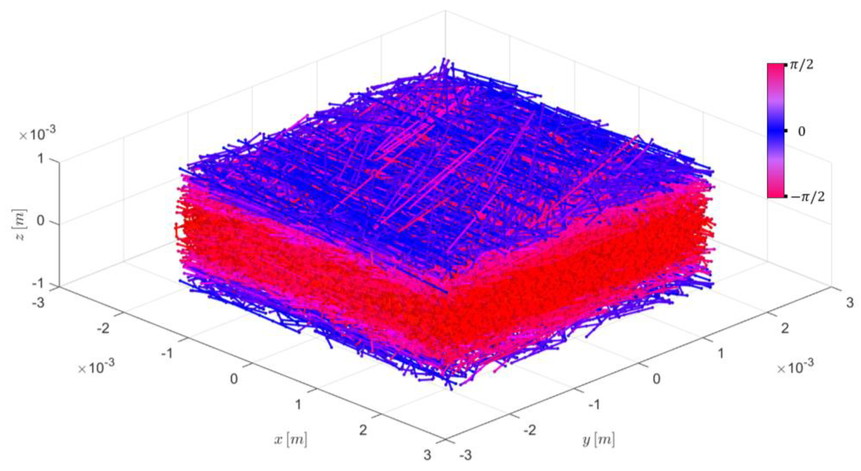
Figure 7.
Computational compression molded cluster, with x as the shearing direction (a11). Fibers are colored as a function of their XY (=12) planar orientation [43].
Figure 7.
Computational compression molded cluster, with x as the shearing direction (a11). Fibers are colored as a function of their XY (=12) planar orientation [43].

Figure 8.
Initial fiber orientation for injection molded samples for simple shear flow tests.

Figure 9.
Experimental (black) and predicted (red) fiber orientation evolution of injection molded samples.
Figure 9.
Experimental (black) and predicted (red) fiber orientation evolution of injection molded samples.

Figure 10.
Smoothed computational a11 evolution of injection molded samples at varying shear strains.
Figure 10.
Smoothed computational a11 evolution of injection molded samples at varying shear strains.

Figure 11.
Experimental (black) and predicted (red) fiber orientation evolution of compression molded samples [43].
Figure 11.
Experimental (black) and predicted (red) fiber orientation evolution of compression molded samples [43].

Figure 12.
Experimental (black) and predicted (red) off-diagonal orientation components (a) a12 and (b) a13 as a function of shear strain.
Figure 12.
Experimental (black) and predicted (red) off-diagonal orientation components (a) a12 and (b) a13 as a function of shear strain.

Figure 13.
Experimental (black) and predicted (red) a11 values averaged through sample thickness at varying shear strains for compression molded samples. (a) Initial fiber orientation distribution at 0 shear strain, (b) fiber orientation distribution after 5 strain units, (c) 12.5, (d) 20, (e) 40, and (f) 60 shear strain units [43].

Figure 14.
Smoothed computational a11 evolution of compression molded samples [43].
Figure 14.
Smoothed computational a11 evolution of compression molded samples [43].


Table 1.
Fiber properties. Average FLs, a11, a22, and a33 as the orientation tensors. a11 representing extrusion direction in compression molded samples and the melt flow direction in injection molded samples.
Table 1.
Fiber properties. Average FLs, a11, a22, and a33 as the orientation tensors. a11 representing extrusion direction in compression molded samples and the melt flow direction in injection molded samples.
| Material Property | CM Plates | IM Plates |
|---|---|---|
| LN [mm] | 0.83 | 1.28 |
| LW [mm] | 1.53 | 2.92 |
| a11 [-] | 0.86 | 0.60 |
| a22 [-] | 0.11 | 0.37 |
| a33 [-] | 0.03 | 0.03 |
Table 2.
Cluster properties for injection- and compression molded samples.
| Cluster Property | IM Plates | CM Plates |
|---|---|---|
| vol % | 4 | 8.5 |
| Longest fiber [mm] | 5 | 4 |
| LN [mm] | 0.71 | 0.83 |
| LW [mm] | 1.32 | 1.53 |
| a11 [-] | 0.6 | 0.36 |
| a22 [-] | 0.39 | 0.62 |
| a33 [-] | 0.002 | 0.02 |
Table 3.
Shear cell properties for injection- and compression molded samples.
| Parameter | Value |
|---|---|
| E [GPa] | 73 |
| Fiber diameter [µm] | 19 |
| η [Pas] | 110 |
| [s−1] | 1 |
| Time step [s] | 5 × 10⁻⁵ |
| Integrations [-] | 1,200,000 |
© 2020 by the authors. Licensee MDPI, Basel, Switzerland. This article is an open access article distributed under the terms and conditions of the Creative Commons Attribution (CC BY) license (http://creativecommons.org/licenses/by/4.0/).
Share and Cite
MDPI and ACS Style
Simon, S.A.; Bechara Senior, A.; Osswald, T. Experimental Validation of a Direct Fiber Model for Orientation Prediction. J. Compos. Sci. 2020, 4, 59. https://0-doi-org.brum.beds.ac.uk/10.3390/jcs4020059
AMA Style
Simon SA, Bechara Senior A, Osswald T. Experimental Validation of a Direct Fiber Model for Orientation Prediction. Journal of Composites Science. 2020; 4(2):59. https://0-doi-org.brum.beds.ac.uk/10.3390/jcs4020059
Chicago/Turabian StyleSimon, Sara Andrea, Abrahán Bechara Senior, and Tim Osswald. 2020. "Experimental Validation of a Direct Fiber Model for Orientation Prediction" Journal of Composites Science 4, no. 2: 59. https://0-doi-org.brum.beds.ac.uk/10.3390/jcs4020059