Boosting Inter-ply Fracture Toughness Data on Carbon Nanotube-Engineered Carbon Composites for Prognostics

Abstract

In order to build predictive analytic for engineering materials, large data is required for machine learning (ML). Gathering such a data can be demanding due to the challenges involved in producing specialty specimen and conducting ample experiments. Additionally, numerical simulations require efforts. Smaller datasets are still viable, however, they need to be boosted systematically for ML. A newly developed, knowledge-based data boosting (KBDB) process, named COMPOSITES, helps in logically enhancing the dataset size without further experimentation or detailed simulation. This process and its successful usage are discussed in this paper, using a combination of mode-I and mode-II inter-ply fracture toughness (IPFT) data on carbon nanotube (CNT) engineered carbon fiber reinforced polymer (CFRP) composites. The amount of CNT added to strengthen the mid-ply interface of CFRP vs the improvement in IPFT is studied. A simpler way of combining mode-I and mode-II values of IPFT to predict delamination resistance is presented. Every step of the 10-step KBDB process, its significance and implementation are explained and the results presented. The KBDB helped in not only adding a number of data points reliably, but also in finding boundaries and limitations of the augmented dataset. Such an authentically boosted dataset is vital for successful ML.

1. Introduction

Advanced polymeric composites are being used in many weight-sensitive, load-carrying applications. Layered configurations, or laminates, are preferred because of flexibility in tailoring properties, optimizing weight and achieving high specific properties [1]. However, exploiting laminate’s full potential is always marred by delamination issues [2].

Researchers have studied inter-ply fracture modes and have suggested a failure criterion based on inter-ply fracture toughness (IPFT), which quantitatively is the strain energy released per unit area (i.e., G kJ/m²) during crack propagation. Loading applied in an opening fracture mode or mode-I is the most damaging. Mode-II is a sliding mode and less detrimental. The tearing mode, commonly known as mode-III, is less of a concern, as the laminates are seen to offer high resistance in this mode. It is likely that most composite laminates experience mixed mode I/II loading in service. Benzeggagh and Kenane [3] suggested a criterion to assess delamination growth under mixed mode I/II as below.

$$G_I+G_{II}=G_{IC}+\left(G_{IIc}-G_{IC}\right)\ast \left[G_{II}/(G_I+G_{II}\right){]}^m$$

(1)

where $G_{IC}$ and $G_{IIc}$ are the critical IPFT in modes I and II, respectively. $G_I$ and $G_{II}$ are the energy release rates in respective modes under mixed mode loading condition. Constant m is an empirical constant. Ali, Amin and Sepideh [4] adopted this formula further and revised it as a failure criterion against delamination. According to them, the total IPFT ($G_{Tc})$ is

$$G_{TC}=G_{IC}+\left(G_{IIc}-G_{IC}\right)\ast \left[G_{II}/(G_I+G_{II}\right){]}^m$$

(2)

In Equation (2), ‘m’ is the Benzeggah and Kenane [3] parameter, which is empirical.

Irrespective of the value of ‘m’, it is clear that $\left[G_{II}/(G_I+G_{II}\right)]<1.0$ when $G_I\ne 0.0$ and $G_{IIc}\ne 0.0$. Thus, in all cases $G_{TC}$ shall lie between $G_{IC}$ and $G_{IIc}$. This also means that one will be able to build a prognostic for possible delamination resistance based on $G_{IC}$ and $G_{IIc}$ values in absence of mixed mode data.

The use of machine learning (ML) in prognostic is widespread in engineering, including composites and materials [5,6,7,8]. Success of ML depends on accurate algorithms and data; in particular, a machine cannot train or learn without data. Such data shall be accurate, and large enough for reliable ML-based predictive analytic for engineering materials like composites. Gathering such data can be demanding, due to the challenges involved in producing special specimen and conducting extensive experiments. Numerical simulation also requires efforts. Smaller datasets, however, may be boosted systematically for ML. Data augmentation works well with images form of data. Statistical methods are helpful, but the accuracy of the generated data cannot be guaranteed, which involves understanding of the engineering materials, parameters, phenomena and even the processes involved. All these warranted a systematic approach to ensure the quality of the new data points (NP).

In this paper, a knowledge-based data boosting (KBDB) process, proposed [9] and discussed [10] by the same author in earlier publications, is adopted. This procedure is meant to address data sparsity systematically and reliably without compromising the data quality. The KBDB process, acrostically named ‘COMPOSITES’ consists of 10 steps that are essential, starting from identifying data, understanding physics, sanitizing available data, to final scrutiny of the boosted dataset. This provides a pragmatic novel way of creating near-real engineering data for ML. KBDB can be adopted for any case that comprises countable variables and quantities, and requires the available lean data to be augmented to the size useful for ML.

A study on IPFT of carbon nanotubes (CNT) engineered carbon fiber reinforced polymer (CFRP) laminates is used to explain and discuss the entire KBDB process. An experimental data highlighting the effect of CNT content on the critical IPFT values is taken from [11] to develop the case study. This original research involved nano-scale strengthening of inter-ply interfaces in CFRP using multi-wall carbon nanotubes (MWCNT) for studying improvement in its IPFT under mode-I and mode-II type of loading. This is still an area under research, offering limited case studies and datasets. For composites, experiments are generally possible only in small numbers, due to the specialty materials, processing and testing methods involved.

The KBDB study presented here facilitated understanding of the data values, operational boundaries, and limitations of the augmented dataset. This demonstrated the utility of the COMPOSITES process for engineering data augmentation.

2. Materials and Methods

A study is conducted for a CFRP composites, a schematic of which is shown in Figure 1. Such composites typically consist of many layers or plies stacked one above the other and cured using heat, vacuum, and pressure to bond the plies together and consolidate them into a laminate.

The inter-ply region between the individual plies is matrix dominated lacking other reinforcement that can resist any form of initiation, formation, and propagation of cracks. The addition of nano-fillers, such as carbon nanotubes (CNT), is seen to improve the resistance to cracks at the inter-ply interfaces [12]. One of the already published [13,14,15,16] research works on such nano-engineered woven CFRP composites from the author’s research group is used in this KBDB exercise.

The specimens were fabricated using a bi-directional, 12 k, plain weave, carbon fabric prepreg that consisted of Epoxy L-930HT matrix. Various type of MWCNT used to nano-reinforce the inter-ply interface were found to bond well with the prepreg [11].

Due to their nano-size, CNT do agglomerate making it difficult to disperse and penetrate into the adjacent plies forming a good reinforcement. In order to achieve uniform dispersion, “dry CNT on transfer media” process was used, as reported in [11,13]. CNT were mixed separately in Ethanol in 1:500 proportion. The mixture was sonicated for 2 hours, and then was spread on a Teflon sheet. After the Ethanol evaporated out, a layer of carbon prepreg was laid on the top such that the CNT stuck onto the prepreg surface in contact. The Teflon sheet was removed after flipping the prepreg upside down. The prepreg layer thus prepared was then stacked in a pre-decided lay-up sequence to form the test laminates. Thin impervious Teflon film used as crack initiator was also laid appropriately. These laminates were cured in an autoclave as recommended by the prepreg supplier [11,13] under 85 psi pressure and 120 deg C temperature for 2 hours. A vacuum of 15–25 mmHg was also applied for debulking and removing volatiles.

Even though CNT agglomeration was eliminated, their spread over the prepreg surface was random, and also, the cutline into the prepreg and the fibers might not have been exactly aligned in all plies. All these might have resulted in the scatter seen in the test results, which was already accounted in for by selecting the minima, mean and maxima values of IPFT. Note that the amount of CNT used varied from 0.0 g/sqm to less than 1.0 g/sqm of the prepreg area.

The DCB and ENF test samples cut from these laminates were used to conduct the tests according to ASTM D 5528 and JIS K7086 respectively [11].

Generation of any engineering data requires understanding of the phenomena and the various parameters involved. Adding new data points to any such available dataset requires the same attention and rigor, especially when the points are to be generated artificially, as before, to uphold the same accuracy. The new knowledge-based data boosting (KBDB) process, reported in [9,10] and used in this paper, is schematically shown in Figure 2.

Below described are these 10 generic steps in the proposed KBDB process. As seen, these also form an acrostic ‘COMPOSITES’ [9,10].

Collect	Gather authentic engineering, semi-processed/raw, data.
Organize	Choose/select data points based on certain parameter or criterion.
Mathematics	Tabulate and plot data points to check scatter, trend and deviation.
Physics	Examine underlying reasons for the data point values.
Oddities	Identify and remove outliers and extremity points.
Space	Mark the space or domain within which the data may be boosted.
Infer	Form guidelines to be observed while boosting the data.
Translate	Form mathematical propositions based on inferred guidelines.
Employ	Apply those propositions to augment the data and visualize it.
Scrutinize	Examine the new dataset considering all details and build suggestions.

The implementation of the process for the CFRP composites case is demonstrated in the next section.

3. Results

In this study, only mode-I and mode-II data for critical IPFT are considered, which are then systematically augmented using the COMPOSITES process.

3.1. Collect:

Double cantilever beam (DCB) and end notched flexure (ENF) test data characterizing mode-I and mode-II IPFT (i.e., $G_{IC}$ and $G_{IIc}$ kJ/m²), respectively, is collected from [11], representing delamination resistance of a bi-directional CFRP composites without nano-fillers and with a variety of CNT added in to strengthen the inter-ply interfaces. The fabrication and testing of the DCB and ENF coupons, for which the data was gathered, were conducted in a controlled environment. A total of five different cases for each mode were identified, where the processing parameters, such as the autoclave curing cycle, applied vacuum as well as sonication period for CNT were consistent. All cases have sufficient scatter. In order to take care of the scatter, all lower-bound, mean and upper-bound values of IPFT are captured as part of the dataset. Out of the five cases for each mode, one is on zero CNT, one with non-functionalized multi-wall (MW) CNT (or MWCNT), and three with functionalized MWCNT with –COOH, –OH1 or –OH2 groups.

3.2. Organize:

The data is arranged such way that the amount of CNT (g/sqm surface of prepreg) used as nano-reinforcement for the mid-plane is directly related to the respective IPFT values. Additionally, the G ratio, $G_{IIc}$/$G_{IC}$, is calculated to understand whether the composites offered more resistance in mode-I or mode-II. This also helps in understanding in which mode the CNT are more effective.

In all total, 30 data points for IPFT and 15 for the G ratio were gathered and plotted in a X-Y domain. The plots for lower, mean, and upper limit values were drawn separately (refer to Figure 3) to get an overall picture of the variations in $G_{IC}$ and $G_{IIc}$ kJ/m² values as a function of weight of CNT per unit area of the inter-ply interface.

This amount of data (15 for each mode) was certainly very lean and not sufficient for any predictive modeling. This certainly required boosting of the entire data set systematically, for which the remaining steps of the COMPOSITES process are implemented.

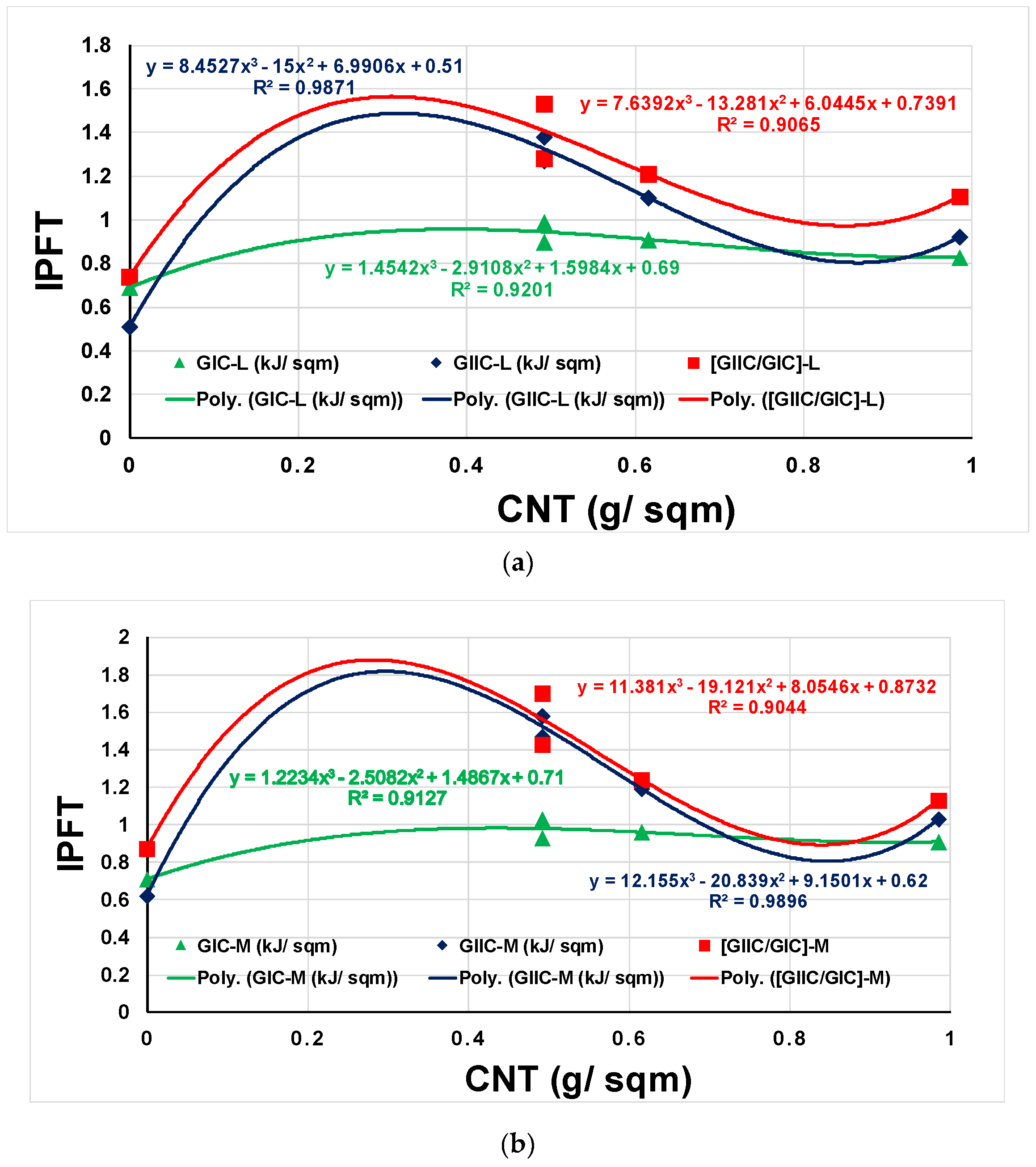
3.3. Mathematics:

It is clear from the data points that the relationship between IPFT and the CNT content is non-linear. Subsequently trend line functions, such as, moving average and polynomials were tried to get the best-fit lines. The third order polynomial functions fit the data in a reasonable manner. The plots are shown in Figure 4. Separate trend lines were plotted for the minima (L), mean (M) and the maxima (U) for clarity and understanding the variance. The trends seemed to best fit and the R² (i.e., Coefficient of Determination, or, in short, CoD) values were high enough in all three cases.

However, the dataset is very sparse and there are intermittent regions of no data, especially where peaks and deeps for the polynomial fits lie. These certainly warrant logical augmentation of the dataset.

3.4. Physics:

It is clear from Figure 4 that, without the addition of CNT, the IPFT in mode-I is slightly higher than in mode-II. However, the CNT changed this trend in that IPFT in mode-II seemed to have improved significantly as compared to IPFT in mode-I. It is certain that with a right proportion of CNT at the inter-ply interface, significant amount of fiber bridging between fibers from the adjacent plies occurs. This fiber bridging helps in sustaining loads for a much longer time, resulting in higher IPFT. In conclusion, the mode-I and mode-II data gathered are representative enough for studying delamination resistance.

It is clear from Equation (2) that, under a mixed mode loading, composites would offer a better resistance than in a pure mode-I condition with a certain amount of CNT added in at the inter-ply interfaces. With this, equation (2) can be simplified as below to derive $G_{TC}$. Equation (3) also satisfies the $G_{IC}\le G_{TC}\le G_{IIC}$ condition.

$$G_{TC}=(G_{IC}\ast z)+G_{IIc}\ast \left(1-z\right) \mathrm{where} 0 > \mathrm{z} > 1$$

(3)

In this study, z = 0.75 is adopted. Figure 5 shows the plots and the trend line equations for the $G_{TC}$ thus calculated; the CoD, in all cases, is excellent.

Although, the way that $G_{TC}$ was calculated might be conservative, still it is more practical than using only single mode values. This also means that for prognostic related to delamination resistance, the ML shall be based on the $G_{TC}$ dataset than $G_{IC}$ and $G_{IIc}$ individually and independently. Notwithstanding, the data augmentation has to be conducted still at the level of individual fracture modes in order to maintain the reliability of the $G_{TC}$ data.

The choice of factor ‘z’ and its impact on the final dataset is discussed later in Section 4.

3.5. Oddities:

As presented in Figure 3, Figure 4 and Figure 5, out of the 15 cases for each mode, three points are the result of zero CNT, three with non-functionalized multi-wall or MWCNT, and nine with functionalized MWCNT with –COOH, –OH₁ or –OH₂. There are six points that belong to the same percentage of MWCNT, but with two different functionlized groups, viz; -COOH and –OH₂. However, the resultant $G_{TC}$ are very close. Therefore, both the data points were retained.

One oddity to observe is the best fit for $G_{IIc}$. Its apex exceeds the maxima of the original dataset (i.e., 1.78 kJ/m²), which does not seem to be realistic. This oddity needs to be and will be scrutinized after the data boosting exercise.

3.6. Space:

It was noticed that beyond 0.6–0.7 g/sqm of CNT content, the gain in IPFT results is minimal. It is mentioned in [11] that CNT content higher than 1 g/sqm thickens the interface, and thereby reduces the IPFT. In the current study, the data values chosen are only up to 0.98 g/sqm of CNT content, hence, that automatically forms the valid limit. In the same way, the minima and maxima of $G_{IC}$ and $G_{IIC}$ data points together (0.51 kJ/m² and 1.78 kJ/m²) form the other limits for the $G_{TC}.$ Thus, it will be good enough to observe these boundaries while data boosting.

3.7. Infer:

Understanding of the data and the physics behind the chosen data points helped in guiding data boosting. First, new $G_{IC},G_{IIC}, and G_{TC}$ data points are to be added in without changing the CNT. In this ‘vertical KBDB’, new points (NP) are to be created in between the minima and mean, as well as the mean and maxima values. This will be linear interpolation. Subsequently, NP to be generated between two close-by CNT content points. It is fair to assume that between any two close-enough points, the variations in $G_{IC} and G_{IIC}$ are linear. This may be termed as ‘horizontal KBDB’. The same may be applied to the diagonally opposite, adjacent data points. These are also the proximity points, one from the L data range and the other from the U data range. This operation is named as ‘cross KBDB’. In summary, the vertical, horizontal and cross KBDB shall logically add NP within the defined space.

These NP creations are justifiable given the fact that the CNT content used in nano-engineering the composites interfaces is small (less than 1 g/sqm), and some variation is expected and bound to happen during actual manufacturing.

3.8. Translate:

The above inferences were then translated into the mathematical simple formulae based on the schematics shown in Figure 6. The effect of these operations can be studied upon generating and adding NP to the original datasets. The trend-lines, their CoD, as well as space boundaries may be examined then.

The cross KBDB can be either forward (as opted in the current case), backward or cross diagonal, which may lead to some variation in data points. This aspect is deliberated in Section 4.

3.9. Employ:

As planned, the NP were created systematically and added to the original dataset. The results for $G_{IC},G_{IIC} and G ratio$ are shown in Figure 7, while the results for $G_{TC}$ are shown in Figure 8.

It is clear from Figure 8 that the KBDB implemented was reasonable, and did not distort the data. It, in fact, helped to fill in empty space rationally closing the gaps in the original data.

3.10. Scrutinize:

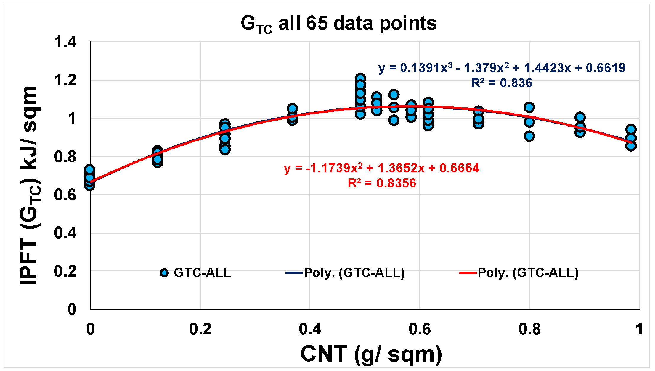
Although the initially collected data was organized in minima, mean and maxima for convenience of analysis, all three points still belonged to only one CNT content. It essentially means that, during predictive modeling, one need not differentiate between L, M and U values. Rather, one can merge all L, M and U values, and use their collective trend for a prognostic. As seen in Figure 9, the entire dataset aligns well irrespective of second or third order trend fitting. In addition, all points fall within the space marked earlier.

This corroborates that all NP are valid and justifiable. The data augmentation factor achieved at this stage through the COMPOSITES approach is 4.33 (i.e., the ratio of augmented dataset of 65 points to the original dataset of 15 values). It was interesting to see how the augmented dataset compared with the original dataset. Referring to Figure 10 for the comparison, it is clear that the dataset augmentation has removed the spuriousness observed in the third order best fit line, due to the sparsity of data.

The second order trend lines have no such issue; however, the CoD for the augmented dataset is better than the original. This will also mean that the boosted dataset follows the original dataset well and will help better facilitate the ML for predictive modeling.

It may also be noted that the second and third order polynomial trend lines show similar trends and CoD values for the new dataset. This is a sort of bench marking and the testimony that the data boosting carried out is reliable. Further error analysis was not conducted since no ML exercise was planned to be part of this study.

4. Discussion

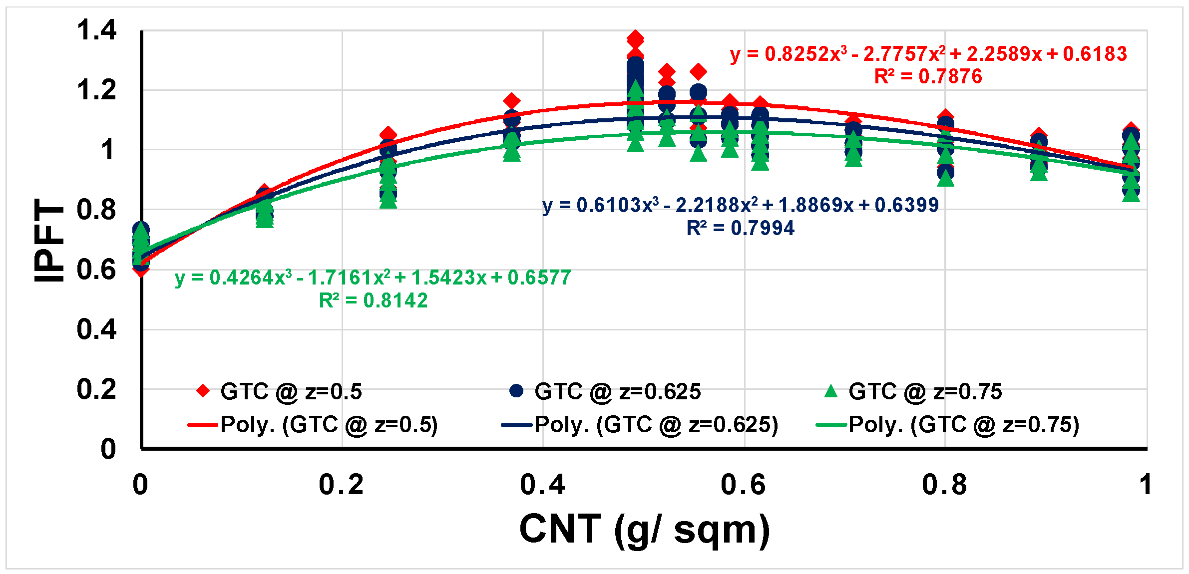
As mentioned earlier, the value of parameter ‘z’ was preselected as 0.75 for this study. This, however, can be changed to fit the loading conditions. For the loading dominated by opening mode, one shall use higher ‘z’ values whereas when loading is closer to sliding mode, ‘z’ shall be low. For mixed mode loading, users may use their preference. Notwithstanding, ‘z’ that gives slightly conservative outcome is always safer.

The final $G_{TC}$ datasets for three different values of ‘z’ are shown in Figure 11. It shows that the shift in trend lines is systematic and logical. This means that the prognostic will remain valid at all such values, as long as the mode-I and mode-II dataset remain the same. The user may even use the same database for either mode-I (z = 1) or mode-II (z = 0) prognostic. This is an added advantage.

As shown in Figure 6, cross KBDB uses forward interpolation. One may alternatively use reversed or X interpolation as shown in Figure 12 to generate NP.

As a result of the small ranges of x and y values, the magnitudes of $G_{IC},G_{IIC}, and G_{TC}$ will, however, not change significantly. In addition, the user may be able to boost the dataset further with additional interpolations within the extent of the original experimental data scatter. However, all these operations fall within the same COMPOSITES approach, and hence are not attempted in this paper.

It may be noted from the polynomial equations in Figure 11 that the fourth or the last term typically indicates the $G_{TC}$ value at zero CNT content (e.g., 0.6577 kJ/m² in Equation 4). The rest of the terms in the same equation, associated with CNT content, give the additional delamination resistance attainable by adding the corresponding amount of CNT at the inter-ply interface.

$$G_{TC}=0.4264({CNT)}^3-1.7161({CNT)}^2+1.5423(CNT)+0.6577 \mathrm{for}\mathrm{z}=0.75$$

(4)

The type of functionalized CNT does have impact on the percentage improvement achievable in $G_{TC}$. However, in this dataset, the variation is within the experimental scatter of the entire dataset. Hence, the user may not need to pay specific attention to the type of functionalization (–COOH, –OH₁ or –OH₂) for the MWCNT to be used.

5. Conclusions

The IPFT data on composites in the study is boosted by a factor 4.33 successfully using the 10-step, COMPOSITES process. This proves the usefulness and versatility of the KBDB process. The new dataset, in fact, became more representative, and both second and third order polynomials seemed to best fit without much variation in CoD. It is demonstrated that this KBDB process not only helped in adding NP to the originally lean dataset, but also helped in identifying and defining the dataset boundaries within the experienced scatter.

Besides this, a simpler way of estimating the total IPFT using the mode-I and mode-II data is presented. This avoided the use of an empirical parameter as used by other researchers. This provided additional flexibility in working with different ratio of mixing between mode-I and mode-II. As such, the same modeling exercise can therefore be used for cases from pure mode I, mixed mode and pure mode II.

References

- Gürdal, Z.; Haftka, R.T.; Hajela, P. Design and Optimization of Laminated Composite Materials; John Wiley & Sons: Hoboken, NJ, USA, 1999. [Google Scholar]
- Sridharan, S. Delamination Behaviour of Composites; Woodhead Publishing and Maney Publishing: Cambridge, UK, 2008. [Google Scholar]
- Benzeggagh, M.L.; Kenane, M. Measurement of mixed-mode delamination fracture toughness of unidirectional glass/epoxy composites with mixed-mode bending apparatus. Compos. Sci. Technol. 1996, 56, 439–449. [Google Scholar] [CrossRef]
- Ali, D.-N.; Amin, F.; Sepideh, R.J. An energy based approach for reliability analysis of delamination growth under mode I, mode II and mixed mode I/II loading in composite laminates. Int. J. Mech. Sci. 2018, 145, 287–298. [Google Scholar] [CrossRef]
- Chen, C.-T.; Gu, G.X. Machine learning for composite materials. MRS Commun. 2019, 9, 556–566. [Google Scholar] [CrossRef] [Green Version]
- Navid, Z.; Johannes, R.; Reza, V. Theory-guided machine learning for damage characterization of composites. Compos. Struct. 2020, 246, 112407. [Google Scholar] [CrossRef]
- Daghigh, V.; Lacy, T.E., Jr.; Daghigh, H.; Gu, G.; Baghaei, K.T.; Mark, F.; Horstemeyer, M.F.; Pittman, C.U., Jr. Machine learning predictions on fracture toughness of multiscale bio-nano-composites. J. Reinf. Plast. Comp. 2020, 39, 587–598. [Google Scholar] [CrossRef]
- Gossett, E.; Toher, C.; Oses, C.; Isayev, O.; Legrain, F.; Rose, F.; Zurek, E.; Carrete, J.; Mingo, N.; Tropsa, A.; et al. AFLOW-ML: A RESTful API for machine-learning predictions of materials properties. Comp. Mater. Sci. 2018, 152, 134–145. [Google Scholar] [CrossRef] [Green Version]
- Joshi, S.C. COMPOSITES: A pragmatic knowledge-based engineering data boosting process. J. Eng. Sci. 2020, 1, 1–2. [Google Scholar]
- Joshi, S.C. Knowledge based data boosting exposition on CNT-engineered carbon composites for machine learning. Adv. Comp. Hybrid. Mat. 2020, 3, 354–364. [Google Scholar] [CrossRef]
- Dikshit, V. Manufacturing and Performance Studies of Laminated Composites with Nano-reinforced Inter-ply Interfaces. Ph.D. Thesis, Nanyang Technological University Singapore, Singapore, 2014. [Google Scholar]
- Fereidoon, A.; Memarian, F.; Ehsani, Z. Effect of CNT on the delamination resistance of composites. Fuller. Nanotub. Carb. Nanostruct. 2013, 21, 712–724. [Google Scholar] [CrossRef]
- Joshi, S.C.; Dikshit, V. Enhancing interlaminar fracture characteristics of woven CFRP prepreg composites through CNT dispersion. J. Comp. Mat. 2011, 46, 665–675. [Google Scholar] [CrossRef]
- Dikshit, V.; Bhudolia, S.K.; Joshi, S.C. Multiscale polymer composites: A review of the interlaminar fracture toughness improvement. Fibers 2017, 5, 38. [Google Scholar] [CrossRef] [Green Version]
- Boon, Y.D.; Joshi, S.C. A review of methods for improving interlaminar interfaces and fracture toughness of laminated composites. Mat. Today Com. 2020, 22, 100830. [Google Scholar] [CrossRef]
- Dikshit, V.; Joshi, S.C. Manufacturing of multiscale interlaminar interface composites and quantitative analysis of interlaminar fracture toughness. In Fiber-Reinforced Nanocomposites: Fundamentals and Applications; Elsevier: New York, NY, USA, 2020; pp. 261–278. [Google Scholar] [CrossRef]
Figure 1.
Schematic of layered composites.
Figure 2.
Schematic of the knowledge-based data boosting (KBDB) process.
Figure 3.
Chosen set of data points, (a) minima or lower-bound, (b) mean or average, (c) maxima or upper-bound, for Mode-I inter-ply fracture toughness.
Figure 4.
Trends and coefficient of determination (CoD) for, (a) minima or lower-bound, (b) mean or average, (c) maxima or upper-bound, Mode-I inter-ply fracture toughness data for carbon fiber reinforced polymer (CFRP).
Figure 5.
Trends and CoD for total inter-ply fracture toughness data for CFRP (a) minima or lower-bound, (b) mean or average, (c) maxima or upper-bound.
Figure 6.
KBDB strategy used for generating (a) vertical, (b) horizontal, and (c) cross new points (NP).
Figure 7.
GIC, GIIC and G ratio values, trends and CoD after the KBDB for (a) minima or lower-bound, (b) mean or average, (c) maxima or upper-bound data.
Figure 8.
GTC (minimum, mean and maximum) values, trends and CoD after the KBDB.
Figure 9.
All GTC values, with second and third order polynomial best fit trends and CoD.
Figure 10.
Comparison between original and augmented GTC datasets, their trends and CoD values (a) third order polynomial trends (b) second order polynomial trends.
Figure 11.
Comparison of all GTC values, with different values of ‘z’ parameter.
Figure 12.
Alternative (a) reversed, (b) X interpolation KBDB strategies for generating cross NP.
Publisher’s Note: MDPI stays neutral with regard to jurisdictional claims in published maps and institutional affiliations. |
© 2020 by the author. Licensee MDPI, Basel, Switzerland. This article is an open access article distributed under the terms and conditions of the Creative Commons Attribution (CC BY) license (http://creativecommons.org/licenses/by/4.0/).
Share and Cite
MDPI and ACS Style
Joshi, S.C. Boosting Inter-ply Fracture Toughness Data on Carbon Nanotube-Engineered Carbon Composites for Prognostics. J. Compos. Sci. 2020, 4, 170. https://0-doi-org.brum.beds.ac.uk/10.3390/jcs4040170
AMA Style
Joshi SC. Boosting Inter-ply Fracture Toughness Data on Carbon Nanotube-Engineered Carbon Composites for Prognostics. Journal of Composites Science. 2020; 4(4):170. https://0-doi-org.brum.beds.ac.uk/10.3390/jcs4040170
Chicago/Turabian StyleJoshi, Sunil C. 2020. "Boosting Inter-ply Fracture Toughness Data on Carbon Nanotube-Engineered Carbon Composites for Prognostics" Journal of Composites Science 4, no. 4: 170. https://0-doi-org.brum.beds.ac.uk/10.3390/jcs4040170