An Assessment of Thick Nanocomposite Plates’ Behavior under the Influence of Carbon Nanotubes Agglomeration

Abstract

The influence assessment of carbon nanotubes (CNTs) agglomeration on CNT-reinforced composite (CNTRC) thick plates’ behavior is the main aim of the present work. CNTs are known to agglomerate into clusters even for relatively low volume fractions, which imposes the need to characterize the effects this may introduce in structures behavior, also knowing that recent works have concluded that neglecting agglomeration phenomenon may lead to an overestimation of the mechanical properties of nanocomposites. Hence, it matters to understand how the arising of these clusters may affect the static and free vibrational behaviors of low side-to-thickness nanocomposite plates. To this purpose, the nanocomposite plate properties’ estimation is performed by using the two-parameter model of agglomeration based on the Eshelby–Mori–Tanaka approach, while for behavioral analyses one considers a Higher-order Shear Deformation Theory (HSDT) based on the displacement field of Kant, implemented through the finite element method. The analyses developed consider a set of parametric studies involving the assessment of the influence of side-to-side ratios, side-to-thickness ratios, boundary conditions, and CNTs’ distributions along the thickness. The results obtained allow concluding that the transverse deflections and fundamental frequencies of these structures are significantly influenced by the CNTs’ agglomeration.

1. Introduction

Carbon nanotubes (CNTs) have excellent mechanical, thermal, and electrical properties, besides their high aspect ratio and large surface area, which make them a desirable material in many engineering applications [1,2,3]. In this work the CNTs are addressed as a reinforcing phase of a polymeric matrix.

Assessing the material properties of a CNTRC is of utmost importance, however using the traditional homogenization schemes for particle-reinforced composites might lead to an over estimation of the material properties, since CNTs tend to bundle together forming inclusions within polymeric matrices, which affects the mechanical properties of the resulting CNTRC, usually in a non-desirable manner. This phenomenon occurs due to their high aspect ratio, van der Waals forces and their low bending stiffness values [4,5,6,7].

To overcome this problem of overestimating the mechanical properties, Shi et al. [8] proposed a theoretical two-parameter agglomeration model using an Eshelby–Mori–Tanaka homogenization scheme. This model is appropriate for modelling the material properties of randomly oriented CNTs within a matrix, based on an equivalent CNT fiber.

The concept of an equivalent long fiber for modelling the properties of the carbon nanotube was developed by Shokrieh [9,10] using the finite element method (FEM) to model the CNT, its interphase region and surrounding resin, treating the interphase region as van der Walls interactions. The equivalent fiber consists in a solid cylindrical nano-fiber and its interphase resin.

Since the proposal of the two-parameter model of agglomeration, a few authors have been exploring this concept of CNTRC properties estimation in late years. Kamarian et al. [11] studied a functionally-graded CNTRC (FG-CNTRC) Timoshenko beam resting on a Paskternak foundation demonstrating that its dynamic behavior is highly influenced by CNTs agglomeration, using the generalized differential quadrature method (GDQ) to formulate the dynamic problem. Another study of the same author [12] revealed the high influence of the agglomeration effect on the natural frequency of CNTRC conical shells using again the GDQ method to solve the governing equations of motion.

Tornabene et al. [13] studied the dynamic behavior of FG-CNTRC doubly-curved shells under the influence of CNTs agglomeration, developing parametric studies involving the CNT volume fraction, agglomeration parameters, and CNTs distribution across the thickness direction to characterize the influence of agglomerated CNTs in the natural frequencies of these structures. Another study developed by the same author [14] addressed the response of CNT-reinforced plates and shells under a static loading and CNTs agglomeration using Carrera Unified Formulation, having this study revealed that the stresses and the strains of these structures were highly affected by the agglomeration effect.

Banić et al. [15] studied the influence of the agglomeration effect on the natural frequencies of CNTRC laminated plates and shells considering an elastic foundation based on the Winkler–Pasternak theory. They concluded that the natural frequencies are highly affected by CNTs agglomeration, with this aspect becoming more evident for higher values of CNTs mass fraction.

Daghigh et al. [16] used the Eringen’s nonlocal elasticity theory to study the bending and buckling response of CNTRC plates resting on a Pasternak elastic foundation under the influence of CNTs agglomeration. They concluded that using an elastic foundation reduced the effect of agglomeration. Previously to this study, the same author had led another study regarding the CNTs agglomeration effect [17] on the dynamic behavior of temperature and size dependent CNTRC plates resting on a viscoelastic foundation using the Pasternak model, where they concluded that ignoring the agglomeration effect might lead to an overestimation of the material properties and the usage of the viscoelastic foundation led to an increase of the natural frequency of the structure.

Yousefi et al. [18] used a combination of the Eshelby–Mori–Tanaka homogenization scheme along with the Hahn’s homogenization technique, and by means of parametric studies they evaluated the influence of CNT agglomeration along with other parameters on the free vibration characteristics of CNT/polymer/fiber laminated truncated conical shells surrounded by an elastic foundation. They confirmed that natural frequencies decreased with the increase of CNTs in agglomerated regions.

The agglomeration effect of continuously graded single-walled CNTs (SWCNTs) on the vibration behavior of a SWCNTs/fiber/polymer/metal laminated cylindrical shell was assessed by Ghasemi et al. [19], by means of parametric studies, evaluating the CNTs’ agglomeration and distribution, mass and volume fraction of the fibers, boundary conditions and lay-up configurations. They concluded that CNT agglomeration significantly affects the natural frequencies and that the symmetric agglomerated CNTs distributions yield higher frequencies.

Kolahchi et al. [20] studied the dynamic response of cylindrical shells submerged in an incompressible fluid subjected to earthquake, thermal, and moisture loads. Several parametric studies were carried out accounting the influences of the fluid, boundary condition, thermal load, moisture changes, structural damping parameter, length to thickness aspect ratio, CNTs volume fraction, and agglomeration state on the dynamic deflections of the structure. The results revealed that when considering the agglomeration effect the deflections increased.

Hassanzadeh-Aghdam et al. [21] investigated the creep response of polymer nanocomposites reinforced with randomly dispersed CNTs through the modelling of a micromechanical model and its comparison with experimental results, which were in excellent agreement. CNTs’ agglomeration as well as the CNT/polymer interphase, were considered in these studies, and it was shown that CNT’s agglomeration dramatically influences and degrades the creep resistance of CNT-reinforced polymers.

On the field of smart structures, Bished et al. [22] addressed wave propagation in CNTRC cylindrical shells with piezoelectric effect under the influence of CNTs agglomeration, and developed and analytical model capable of finding the effects of CNTs agglomeration on wave propagation characteristics in applications of energy harvesting and structural health monitoring.

Continuing with the advances in CNT-reinforced piezoelectric materials, Krishnaswamy et al. [23] studied piezoelectric matrix inclusion composites using lead-free ceramic, and developed a modelling paradigm to improve the piezoelectric effect by means of optimal polycrystallinity and improved matrices in the considered piezoelectric inclusions. CNTs were included within the matrices with the objective of improving the piezoelectric response. Although CNT agglomeration has been shown as undesirable by many studies, here they have shown that under certain circumstances these inclusions can lead to an enhancement of the piezoelectric effect.

Moradi-Dastjerdi et al. [24] bonded the upper and the lower surfaces of CNTRC porous plate with piezoceramics and studied the deflection and the stress responses under static mechanical and electrical solicitations. They concluded that introducing CNTs in the middle lamina had a positive effect in the deflections of the nanocomposite plate, however only up to a certain CNTs volume fraction due to CNTs agglomeration effect.

A recent review article reinforced that this agglomeration effect directly affects CNTRC thermal, electrical, and mechanical properties. It is also mentioned that there are already a few effective CNT dispersion methods that may contribute to reduce the clustering, but re-agglomeration is still common with the increase of contamination of the material [25].

In a previous work, the present authors [26] developed parametric studies on the natural frequencies and modes’ shapes of thin and moderately thick FG-CNTRC square and rectangular plates under the influence of CNTs agglomeration using a first-order shear deformation theory (FSDT) to formulate the governing equations of motion of the problem. It was concluded that the agglomeration negatively affects the natural frequencies of these structures, but also influence certain modes’ shapes for a few CNTs distributions.

The CNTs have entered the fields of engineering due to their superior physical properties. However, they tend to bundle together negatively affecting their mechanical properties and not taking into account this agglomeration effect might lead to an overestimation of its properties, even for relatively low volume fractions [27], as already highlighted by the several studies mentioned above. In this work one assesses the static and free vibration behaviors of thick FG-CNTRC quadrilateral-shaped plates, using for this purpose a Higher-order Shear Deformation Theory (HSDT) model. The influence of the CNT agglomeration in these nanocomposite plates namely the deterioration effect it has on the mechanical behavior of these structures is addressed in order to prevent overestimated numerically predicted responses. The influence of the CNT’s distributions through these thick structures thickness is also addressed considering the potential relevance they may provide to the plates’ response.

2. Materials and Methods

This section aims to do a brief description of the models, techniques, and methodologies used in the present work. This section is divided in two main sub-sections, a first one where the two-parameter agglomeration model using the Eshelby–Mori–Tanaka approach is used for properties’ prediction purpose and the second one devoted to the model development based on a HSDT theory.

2.1. Two Parameter Agglomeration Model Based on the Eshelby–Mori–Tanaka Approach

As mentioned in the introduction, CNTs have a tendency to agglomerate together forming clusters in the polymeric matrices because of their high aspect ratio, van der Waals forces interaction, and low bending stiffness [4,5,27].

For the present study, the property estimation is based on the two-parameter agglomeration model based on the Eshelby–Mori–Tanaka approach described for the first time by Shi et al. [8], which is based on an equivalent fiber concept. The equivalent fiber properties may be determined using a multiscale finite element method (FEM) analysis or by molecular dynamics’ (MD) simulations. These FEM or MD simulations will yield the properties of the composite.

$$\{\begin{array}{c}{E}_{LEF}=\frac{E_{LC}}{V_{EF}}-\frac{E_M{V}_M}{V_{EF}}\\ \frac{1}{E_{TEF}}=\frac{1}{E_{TC}{V}_{EF}}-\frac{V_M}{E_M{V}_{EF}}\\ \frac{1}{G_{EF}}=\frac{1}{G_C{V}_{EF}}-\frac{V_M}{G_M{V}_{EF}}\\ {\nu }_{EF}=\frac{{\nu }_C}{V_{EF}}-\frac{{\nu }_M{V}_M}{V_{EF}}\end{array}$$

(1)

The properties can be determined using the Rule of Mixtures (ROM), presented in Equation (1), where $E_{LEF}$, $E_{TEF}$, $G_{EF}$, and ${\nu }_{EF}$ are the longitudinal elastic modulus, transverse elastic modulus, transverse shear modulus and the Poisson’s ratio of the equivalent fiber. The constants $E_{LC}$, $E_{TC}$, $G_C$, and ${\nu }_C$ are respectively the longitudinal elastic modulus, transverse elastic modulus, transverse shear modulus and the Poisson’s ratio of the composite determined using FEM or MD, and finally, $E_M$, $G_M$, and ${\nu }_M$ are the elastic modulus, the shear modulus and the Poisson’s ration of the matrix. The volume fraction of the matrix and equivalent fiber are denoted by $V_M$ and $V_{EF}$, respectively.

The virtual equivalent fiber consists of a straight CNT embedded in a polymeric resin and its interphase [9]. For the present study, a SWCNT is considered with a chiral index of (10,10) and its equivalent fiber is defined by a solid cylinder with 1.424 nm of diameter [11]. The properties of this equivalent fiber are listed in the

Table 1. Properties of the equivalent fiber considered [11].

Properties	Value
Longitudinal elastic modulus (GPa)	649.12
Transverse elastic modulus (GPa)	11.27
Transverse shear modulus (GPa)	5.13
Poisson’s ratio	0.284
Density (kg/m3)	1400

.

The agglomeration model based on the Eshelby–Mori–Tanaka homogenization scheme considers that the CNTs are randomly dispersed along the matrix, but some of them are known to be bundled together forming clusters. Those clusters or inclusions are modelled according to the Eshelby inclusion model, considering these inclusions will assume a spherical shape [11], as schematically represented in Figure 1.

The detailed description of the present two-parameter model of agglomeration can be found in the reference article written by Shi et al. [8].

The total CNT volume fraction in the representative volume element (RVE) is denotes by $V_r$ and is divided in the volume fraction of CNTs inside the inclusions $V_r^{inclusion}$ and in the CNTs volume fraction outside the inclusions and dispersed in the matrix $V_r^m$, thus one can express the total CNT volume fraction in the RVE according to

$$V_r=V_r^{inclusion}+V_r^m$$

(2)

The agglomeration state is described according to two parameters, $\mu$ which is the volume fraction of inclusions ($V_{inclusion}$) considering the volume $V$ of the RVE, and $\eta$ which is the volume ratio between of the volume of CNTs that are within the inclusions and the total volume of CNTs in the RVE.

When $\mu =1$ or $\mu =\eta$ the CNTs are uniformly distributed along the matrix. When $\mu$ decreases; the level of agglomeration in the CNTRC becomes more severe. When $\eta =1$, all CNTs in the CNTRC are located within inclusions which is a state of complete agglomeration; however, it is more common to incur in a partial agglomeration situation [8], where both parameters characterize the agglomerated state. If $\eta >\mu$ and for high values of $\eta$, the CNTs’ distribution throughout the matrix is more heterogeneous.

$$\mu =\frac{V_{inclusion}}{V}, \eta =\frac{V_r^{inclusion}}{V_r}$$

(3)

Although the CNTs are assumed to be transversely isotropic, given the nanoscale of these particles and considering that they are randomly distributed throughout the matrix, as well as within the spherical inclusions, one can consider that the CNTRC behaves as an isotropic material inside and outside the inclusions. The subscript $r$ stands for the reinforcing phase and the subscript $m$ stands for the matrix phase. Generally, the average volume fraction of CNTs $f_r$ in the material is expressed by

$$f_r=\frac{V_r}{V}$$

(4)

This homogenization scheme uses the Hill’s elastic moduli $n_r$, $l_r$, $k_r$, $m_r$, and $p_r$ of the equivalent fiber for property estimation. The Hill’s elastic moduli of the equivalent fiber can be determined using the values of the inverse of the compliance matrix, given by [11]:

$$C_r=\left[\begin{array}{cccccc}{n}_r& l_r& l_r& 0& 0& 0\\ l_r& k_r+m_r& k_r-m_r& 0& 0& 0\\ l_r& k_r-m_r& k_r+m_r& 0& 0& 0\\ 0& 0& 0& p_r& 0& 0\\ 0& 0& 0& 0& m_r& 0\\ 0& 0& 0& 0& 0& p_r\end{array}\right]={\left[\begin{array}{cccccc}\frac{1}{E_L}& -\frac{{\nu }_{TL}}{E_T}& -\frac{{\nu }_{ZL}}{E_Z}& 0& 0& 0\\ -\frac{{\nu }_{LT}}{E_L}& \frac{1}{E_T}& -\frac{{\nu }_{ZT}}{E_Z}& 0& 0& 0\\ -\frac{{\nu }_{LZ}}{E_L}& -\frac{{\nu }_{TZ}}{E_T}& \frac{1}{E_Z}& 0& 0& 0\\ 0& 0& 0& \frac{1}{G_{TZ}}& 0& 0\\ 0& 0& 0& 0& \frac{1}{G_{TZ}}& 0\\ 0& 0& 0& 0& 0& \frac{1}{G_{LT}}\end{array}\right]}^{-1}$$

(5)

The $E_L$, $E_T$, $E_Z$, $G_{LT}$, $G_{TZ}$, $G_{TZ}$, and ${\nu }_{LT}$ are the equivalent fiber properties. In the next step, the effective bulk modulus inside $K_{in}$ and outside $K_{out}$ the inclusions, as well as the shear elastic modulus inside $G_{in}$ and outside $G_{out}$ the inclusions, will be determined according to:

$$K_{in}=K_m+\frac{f_r\eta \left({\delta }_r-3K_m{\alpha }_r\right)}{3\left(\mu -f_r\eta +f_r\eta {\alpha }_r\right)}$$

(6)

$$K_{out}=K_m+\frac{f_r\left(1-\eta \right)\left({\delta }_r-3K_m{\alpha }_r\right)}{3\left[1-\mu -f_r\left(1-\eta \right)+f_r\left(1-\eta \right){\alpha }_r\right]}$$

(7)

$$G_{in}=G_m+\frac{f_r\eta \left({\eta }_r-2G_m{\beta }_r\right)}{2\left(\mu -f_r\eta +f_r\eta {\beta }_r\right)}$$

(8)

$$G_{out}=G_m+\frac{f_r\left(1-\eta \right)\left({\eta }_r-2G_m{\beta }_r\right)}{2\left[1-\mu -f_r\left(1-\eta \right)+f_r\left(1-\eta \right){\beta }_r\right]}$$

(9)

where

$${\alpha }_r=\frac{3\left(K_m+G_m\right)+k_r-l_r}{3\left(K_m+k_r\right)}$$

(10)

$${\beta }_r=\frac{1}{5}\left\{\frac{4G_m+2k_r+l_r}{3(G_m+k_r)}+\frac{4G_m}{G_m+p_r}+\frac{2\left[G_m\left(3K_m+G_m\right)+G_m\left(3K_m+7G_m\right)\right]}{G_m\left(3K_m+G_m\right)+m_r\left(3K_m+7G_m\right)}\right\}$$

(11)

$${\delta }_r=\frac{1}{3}\left[n_r+2l_r+\frac{\left(2k_r+l_r\right)\left(3K_m+2G_m-l_r\right)}{G_m+k_r}\right]$$

(12)

$${\eta }_r= \frac{1}{5}\left[\frac{2}{3}\left(n_r-l_r\right)+\frac{8G_m{p}_r}{G_m+p_r}+\frac{8m_r{G}_m\left(3K_m+4G_m\right)}{3K_m\left(G_m+p_r\right)+G_m\left(7m_r+G_m\right)}+\frac{2\left(k_r-l_r\right)\left(2G_m+l_r\right)}{3(G_m+k_r)}\right]$$

(13)

$K_m$ and $G_m$ are the bulk modulus and the shear modulus of the matrix phase, respectively. Finally, the effective mechanical properties of the CNTRC are expressed according to

$$K=K_{out}\left[1+\frac{\mu \left(\frac{K_{in}}{K_{out}}-1\right)}{1+\alpha \left(1-\mu \right)\left(\frac{K_{in}}{K_{out}}-1\right)}\right]$$

(14)

$$G=G_{out}\left[1+\frac{\mu \left(\frac{G_{in}}{G_{out}}-1\right)}{1+\beta \left(1-\mu \right)\left(\frac{G_{in}}{G_{out}}-1\right)}\right]$$

(15)

where $K$ is the effective bulk modulus and $G$ is the effective shear modulus of the CNTRC material, and the ${\nu }_{out}$ (Possoin’s ratio outside the inclusions), $\alpha$ and $\beta$ are given by

$${\nu }_{out}=\frac{\left(3K_{out}-2G_{out}\right)}{2\left(3K_{out}+2G_{out}\right)}$$

(16)

$$\alpha =\frac{1+{\nu }_{out}}{3\left(1-{\nu }_{out}\right)}$$

(17)

$$\beta =\frac{2\left(4-5{\nu }_{out}\right)}{15\left(1-{\nu }_{out}\right)}$$

(18)

The effective Young’s modulus and Poisson’s ratio of the CNTRC are given according to

$$E=\frac{9KG}{3K+G}$$

(19)

$$\nu =\frac{3K-2G}{6K+2G}$$

(20)

The mass density of the CNTRC $\rho$ is calculated using the Voigt’s rule of mixtures, [28,29], where ${\rho }_m$ is the mass density and $f_m=1-f_r$ is the volume fraction of the matrix phase:

$$\rho =f_r{\rho }_r+f_m{\rho }_m$$

(21)

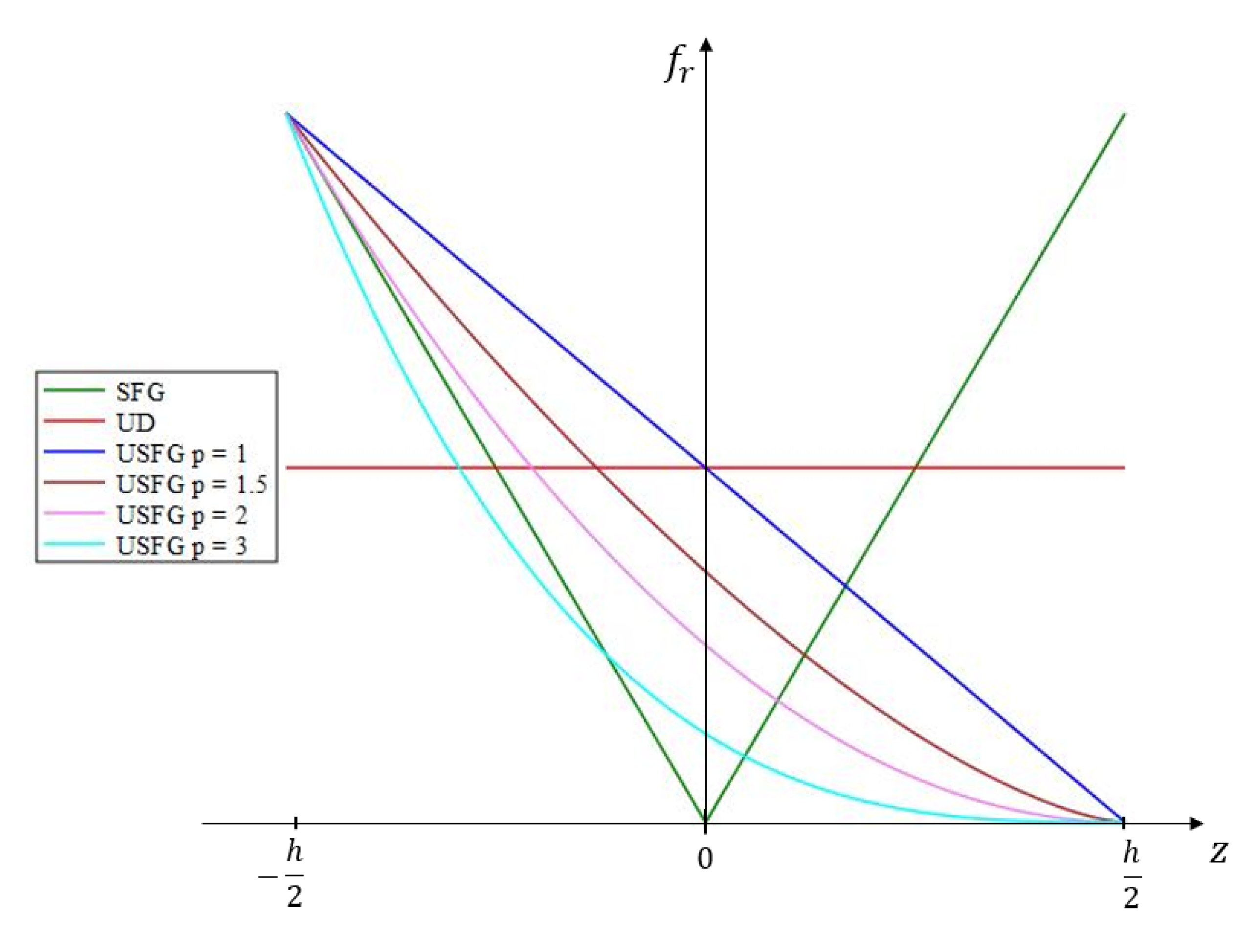
In the present study, different CNT volume fraction distributions along the thickness were considered. The functions that model the considered distributions are presented in the

Table 2. Carbon nanotubes (CNTs) volume fraction distributions considered.

CNTs Distributions
uniformly distributed (UD)	$f_r=f_r^{*}$
symmetrically functionally graded (SFG)	$f_r=\frac{4·\left|z\right|}{h}{f}_r^{*}$
unsymmetrically functionally graded (USFG)	$f_r=2·f_r^{*}{\left(\frac{1}{2}-\frac{z}{h}\right)}^p$

, where UD stands for uniformly distributed, SFG stands for symmetrically functionally graded, and finally, USFG stands for unsymmetrically functionally graded and obeys to a power law of reinforcement distribution. In the present study, the exponent of the USFG distribution is assumed the values of $p=\left\{1,1.5, 2, 3\right\}$.

The coordinate in the thickness direction varies within the interval $\left[-\frac{h}{2},\frac{h}{2}\right]$, where $h$ is the thickness of the plate and $f_r^{*}$ is expressed by

$$f_r^{*}=\frac{w_r}{w_r+\left(\frac{{\rho }_r}{{\rho }_m}\right)-\left(\frac{{\rho }_r}{{\rho }_m}\right)w_r}$$

(22)

where $w_r$ is the mass fraction of the CNTs. For the distributions considered, the CNT volume fraction varies across thickness according to the graphical representation of the Figure 2. Observing the graphical representation, it becomes clear that when p > 1, the CNT total volume in the CNTRC will be less when comparing to the other distributions.

2.2. Static and Free Vibration Analyses of Thick Plates

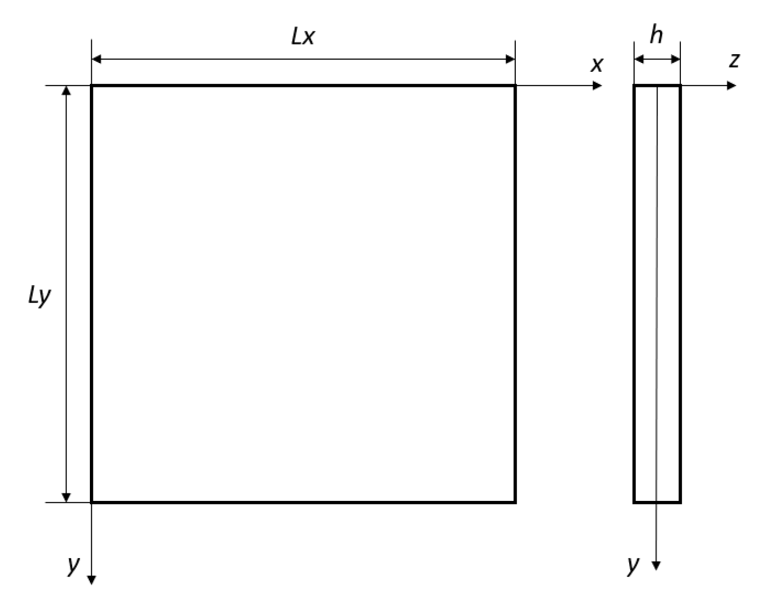
This work aims to characterize the static and free vibration behaviors of square and rectangular thick plates reinforced with agglomerated CNTs in a polymeric matrix. Finite element models were developed using a higher-order theory based on the HSDT of Kant [30,31]. The plate model with generic dimensions is presented in the Figure 3.

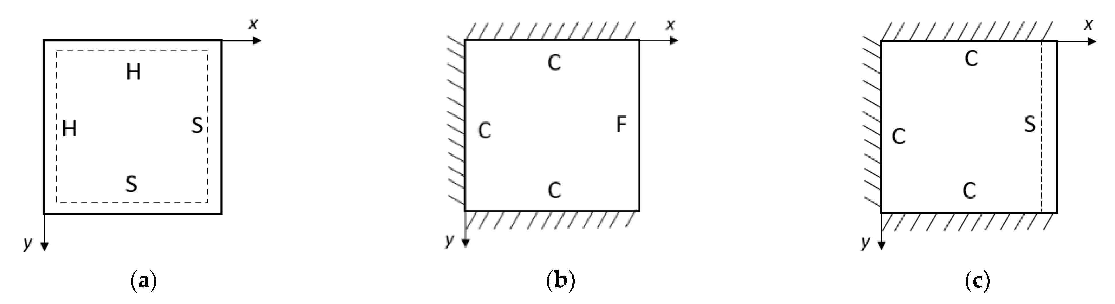
Three different boundary conditions were considered, as illustrated in the Figure 4, where C stands for clamped, F stands for free, H stands for hinged and S for supported. The difference between the hinged and the supported condition is in the constriction of the translational degrees of freedom $u^0$ and $v^0$, where for the hinged condition they are restricted and for the supported condition they are not, and for the sake of simplicity the (a) case will be denoted as simply-supported (SSSS).

The aspect ratio between the length of the $x$-edge and the thickness of the plate is considered to be $\raisebox{1ex}{$L_x$}\!\left/ \!\raisebox{-1ex}{$h$}\right.=5$, and the relations between the $x$ and $y$ edges’ lengths are $\raisebox{1ex}{$L_x$}\!\left/ \!\raisebox{-1ex}{$L_y$}\right.=\left\{1,2,3\right\}$.

2.2.1. Constitutive Equations

The present HSDT has the following displacement field, and is based on the HSDT of Kant [30,31]:

$$\begin{array}{c}u\left(x,y,z\right)=u^0\left(x,y,t\right)+z{\theta }_x\left(x,y,t\right)+z^3{\theta }_x^{*}\left(x,y,t\right)\\ v\left(x,y,z\right)=v^0\left(x,y,t\right)+z{\theta }_y\left(x,y,t\right)+z^3{\theta }_y^{*}\left(x,y,t\right)\\ w\left(x,y,z,t\right)=w^0\left(x,y,t\right)\end{array}$$

(23)

where ${\theta }_x$ and ${\theta }_y$ are the first order rotations, ${\theta }_x^{*}$ and ${\theta }_y^{*}$ are the third order rotations, and the $u^0$, $v^0$ and $w^0$ are the mid-surface displacements in the $\left(x,y,z\right)$ directions, respectively, and $t$ denotes time. Note that the original Kant theory does not consider the translational displacements $u^0$ and $v^0$, and the displacement w(x,y,z,t) is not necessarily constant along the thickness. The superscript 0 is used to refer to the mid-surface of the plate. The present displacement field presents a greater similarity with the version proposed by Pandya and Kant [31], which does not consider the $w\left(x,y,z,t\right)$ variable through-thickness.

The vector of the degrees of freedom {u} in the present work is defined as

$$\left\{u\right\}={\left\{\begin{array}{ccccccc}{w}^0& {\theta }_x& {\theta }_y& {\theta }_x^{*}& {\theta }_y^{*}& u^0& v^0\end{array}\right\}}^T$$

(24)

The strains of the present HSDT are obtained by considering the elasticity kinematical relations for small deformations [32,33]:

$$\left\{\begin{array}{c}{ϵ}_{xx}\\ {ϵ}_{yy}\\ {\gamma }_{xy}\\ {\gamma }_{yz}\\ {\gamma }_{xz}\end{array}\right\}=\left\{\begin{array}{c}\frac{\partial u}{\partial x}\\ \frac{\partial v}{\partial y}\\ \frac{\partial u}{\partial y}+\frac{\partial v}{\partial x}\\ \frac{\partial y}{\partial z}+\frac{\partial w}{\partial y}\\ \frac{\partial u}{\partial z}+\frac{\partial w}{\partial x}\end{array}\right\}$$

(25)

where ${ϵ}_{xx}$, ${ϵ}_{yy}$, and ${\gamma }_{xy}$ are the in-plane normal and shear strain components, ${\gamma }_{yz}$ and ${\gamma }_{xz}$ are the transverse shear strain components, which for the present HSDT yields, [31,33]:

$$\begin{array}{c}\left\{ϵ\right\}=\left\{\begin{array}{c}{ϵ}_{xx}\\ {ϵ}_{yy}\\ {\gamma }_{xy}\end{array}\right\}=\left\{\begin{array}{c}\frac{\partial u^0}{\partial x}\\ \frac{\partial v^0}{\partial y}\\ \frac{\partial u^0}{\partial y}+\frac{\partial v^0}{\partial x}\end{array}\right\}+z\left\{\begin{array}{c}\frac{\partial {\theta }_x}{\partial x}\\ \frac{\partial {\theta }_y}{\partial y}\\ \frac{\partial {\theta }_x}{\partial y}+\frac{\partial {\theta }_y}{\partial x}\end{array}\right\}+z^3\left\{\begin{array}{c}\frac{\partial {\theta }_x^{*}}{\partial x}\\ \frac{\partial {\theta }_y^{*}}{\partial y}\\ \frac{\partial {\theta }_x^{*}}{\partial y}+\frac{\partial {\theta }_y^{*}}{\partial x}\end{array}\right\},\\ \left\{\gamma \right\}=\left\{\begin{array}{c}{\gamma }_{yz}\\ {\gamma }_{xz}\end{array}\right\}=\left\{\begin{array}{c}\frac{\partial w^0}{\partial y}+{\theta }_y\\ \frac{\partial w^0}{\partial x}+{\theta }_x\end{array}\right\}+3z^2\left\{\begin{array}{c}{\theta }_x^{*}\\ {\theta }_y^{*}\end{array}\right\}\end{array}$$

(26)

Considering the present CNTRC material behaves as an isotropic material and the higher order theory used, the strain field is related to the stresses by the constitutive equation:

$$\begin{array}{c}\left\{\sigma \right\}=\left[Q\right]\left\{ϵ\right\}\\ \left\{\begin{array}{c}{\sigma }_{xx}\\ {\sigma }_{yy}\\ {\tau }_{xy}\\ {\tau }_{yz}\\ {\tau }_{xz}\end{array}\right\}=\left[\begin{array}{ccccc}{Q}_{11}& Q_{12}& 0& 0& 0\\ Q_{12}& Q_{22}& 0& 0& 0\\ 0& 0& Q_{66}& 0& 0\\ 0& 0& 0& Q_{44}& 0\\ 0& 0& 0& 0& Q_{55}\end{array}\right]\left\{\begin{array}{c}{ϵ}_{xx}\\ {ϵ}_{yy}\\ {\gamma }_{xy}\\ {\gamma }_{yz}\\ {\gamma }_{xz}\end{array}\right\}\end{array}$$

(27)

being the elastic stiffness coefficients associated to $\left[Q\right]$ given as

$$\begin{array}{c}{Q}_{11}=Q_{22}=\frac{E}{1-{\nu }^2}\\ Q_{12}=\frac{\nu E}{1-{\nu }^2}\\ Q_{44}=Q_{55}=Q_{66}=G\end{array}$$

(28)

where $E$, v and $G$ are the Young’s modulus, the Poisson’s ratio, and the transverse shear modulus, respectively, of the CNTRC.

2.2.2. Hamilton’s Principle

The Hamilton’s principle can be generally stated for a time interval between $t0$ and $t1$ as [29]:

$$\delta \underset{t0}{\overset{t1}{{\displaystyle \int }}}\left(\left(T-U\right)+W\right)dt=0$$

(29)

with $T$ standing for the kinetic energy, $U$ for the elastic strain energy, and $W$ for the work performed by applied forces, generically described according to

$$\begin{array}{c}T=\frac{1}{2}{{\displaystyle \int }}_V^{}\rho \left({\dot{u}}^2+{\dot{v}}^2+{\dot{w}}^2\right)dV\\ U=\frac{1}{2}{{\displaystyle \int }}_V^{}\left({\left\{ϵ\right\}}^T\left\{\sigma \right\}+{\left\{\gamma \right\}}^T\left\{\tau \right\}\right) dV\\ W={{\displaystyle \int }}_A^{}{\left\{q\right\}}^T·\left\{u\right\} dA\end{array}$$

(30)

in which, $\rho$ is the mass density of the material, $\dot{u}$, $\dot{v}$, and $\dot{w}$ are the velocities, and $\left\{q\right\}$ is the load vector.

Considering the aim of performing static analyses, the equilibrium equation obtained after a few mathematical manipulations, for the whole discretized domain, is given as

$$\left[K\right]\left\{u\right\}-\left\{f\right\}=0$$

(31)

where $\left\{u\right\}$ is the displacement vector, $\left[K\right]$ is the global stiffness matrix and $\left\{f\right\}$ is the load vector. The global stiffness matrix can be seen as constituted by a set of contributed matrices concerning different effects, namely, ${\left[K_{bb}\right]}^e$, ${\left[K_{b{b}^{*}}\right]}^e$, ${\left[K_{b^{*}b}\right]}^e$, ${\left[K_{b^{*}{b}^{*}}\right]}^e$, ${\left[K_{mm}\right]}^e$, ${\left[K_{ss}\right]}^e$, ${\left[K_{s^{*}s}\right]}^e$, ${\left[K_{s{s}^{*}}\right]}^e$, and ${\left[K_{s^{*}{s}^{*}}\right]}^e$ which stand for the stiffness matrices with the first order bending-bending terms, first order bending and higher-order bending terms, higher-order bending and first order bending terms, higher-order bending-bending terms, membrane-membrane terms, first order shear-shear terms, higher-order shear and first order shear terms, first order shear and higher-order shear terms, and higher-order shear-shear terms, respectively.

$$\left[K\right]={\displaystyle \sum }_{e=1}^N\left({\left[K_{bb}\right]}^e+{\left[K_{b{b}^{*}}\right]}^e+{\left[K_{b^{*}b}\right]}^e+{\left[K_{b^{*}{b}^{*}}\right]}^e+{\left[K_{mm}\right]}^e+{\left[K_{ss}\right]}^e+{\left[K_{s^{*}s}\right]}^e+{\left[K_{s{s}^{*}}\right]}^e+{\left[K_{s^{*}{s}^{*}}\right]}^e\right)$$

(32)

The index $e$ refers to a given element and $N$ is the total number of elements, in which the structure domain is sub-divided. These matrices are calculated according to the following expressions, where $\left(\xi ,\eta \right)$ are the local coordinates within each element [31,34]:

$${\left[K_{bb}\right]}^e=\underset{-1}{\overset{1}{{\displaystyle \int }}}\underset{-1}{\overset{1}{{\displaystyle \int }}}{\left[B_b\right]}_e^T{\left[D\right]}_{i,j=1,2,6}{\left[B_b\right]}_e\det \left(\left[J_e\right]\right) d\xi d\eta$$

(33)

$${\left[K_{mm}\right]}^e=\underset{-1}{\overset{1}{{\displaystyle \int }}}\underset{-1}{\overset{1}{{\displaystyle \int }}}{\left[B_m\right]}_e^T{\left[A\right]}_{i,j=1,2,6}{\left[B_m\right]}_e\det \left(\left[J_e\right]\right) d\xi d\eta$$

(34)

$${\left[K_{b^{*}b}\right]}^e=\underset{-1}{\overset{1}{{\displaystyle \int }}}\underset{-1}{\overset{1}{{\displaystyle \int }}}{\left[B_{b^{*}}\right]}_e^T{\left[F\right]}_{i,j=1,2,6}{\left[B_b\right]}_e\det \left(\left[J_e\right]\right) d\xi d\eta$$

(35)

$${\left[K_{b{b}^{*}}\right]}^e=\underset{-1}{\overset{1}{{\displaystyle \int }}}\underset{-1}{\overset{1}{{\displaystyle \int }}}{\left[B_b\right]}_e^T{\left[F\right]}_{i,j=1,2,6}{\left[B_{b^{*}}\right]}_e\det \left(\left[J_e\right]\right)d\xi d\eta$$

(36)

$${\left[K_{b^{*}{b}^{*}}\right]}^e=\underset{-1}{\overset{1}{{\displaystyle \int }}}\underset{-1}{\overset{1}{{\displaystyle \int }}}{\left[B_{b^{*}}\right]}_e^T\left[H\right]{\left[B_{b^{*}}\right]}_e\det \left(\left[J_e\right]\right) d\xi d\eta$$

(37)

$${\left[K_{ss}\right]}^e=\underset{-1}{\overset{1}{{\displaystyle \int }}}\underset{-1}{\overset{1}{{\displaystyle \int }}}{\left[B_s\right]}_e^T{\left[A\right]}_{i,j=4,5}{\left[B_s\right]}_e\det \left(\left[J_e\right]\right) d\xi d\eta$$

(38)

$${\left[K_{s^{*}s}\right]}^e=\underset{-1}{\overset{1}{{\displaystyle \int }}}\underset{-1}{\overset{1}{{\displaystyle \int }}}{\left[B_{s^{*}}\right]}_e^T{\left[D\right]}_{i,j=4,5}{\left[B_s\right]}_e\det \left(\left[J_e\right]\right) d\xi d\eta$$

(39)

$${\left[K_{s{s}^{*}}\right]}^e=\underset{-1}{\overset{1}{{\displaystyle \int }}}\underset{-1}{\overset{1}{{\displaystyle \int }}}{\left[B_s\right]}_e^T{\left[D\right]}_{i,j=4,5}{\left[B_{s^{*}}\right]}_e\det \left(\left[J_e\right]\right)d\xi d\eta$$

(40)

$${\left[K_{s^{*}{s}^{*}}\right]}^e=\underset{-1}{\overset{1}{{\displaystyle \int }}}\underset{-1}{\overset{1}{{\displaystyle \int }}}{\left[B_{s^{*}}\right]}_e^T{\left[F\right]}_{i,j=4,5}{\left[B_{s^{*}}\right]}_e\det \left(\left[J_e\right]\right)d\xi d\eta$$

(41)

Similarly to the global stiffness matrix, the load vector $\left\{f\right\}$ is obtained calculating the load contribution on each element, where $\left\{N\right\}$ is the vector containing the interpolating functions of the element $e$ [33]:

$${\left\{f\right\}}^e=\underset{-1}{\overset{1}{{\displaystyle \int }}}\underset{-1}{\overset{1}{{\displaystyle \int }}}{\left\{N\left(\xi ,\eta \right)\right\}}^T·\left\{q\right\}·\det \left(\left[J_e\right]\right)d\xi d\eta$$

(42)

where $\left[A\right]$, $\left[D\right]$, [F], and [H] are the extensional stiffness, first order bending stiffness, the first and higher-order bending coupling stiffness and the higher-order stiffness matrices, and their components are calculated according to

$$A_{ij}=\underset{-\raisebox{1ex}{$h$}\!\left/ \!\raisebox{-1ex}{$2$}\right.}{\overset{\raisebox{1ex}{$h$}\!\left/ \!\raisebox{-1ex}{$2$}\right.}{{\displaystyle \int }}}{\overline{Q}}_{ij}dz i,j=1,\dots , 6$$

(43)

$$D_{ij}=\underset{-\raisebox{1ex}{$h$}\!\left/ \!\raisebox{-1ex}{$2$}\right.}{\overset{\raisebox{1ex}{$h$}\!\left/ \!\raisebox{-1ex}{$2$}\right.}{{\displaystyle \int }}}{z}^2·{\overline{Q}}_{ij}dz i,j=1,\dots , 6$$

(44)

$$F_{ij}=\underset{-\raisebox{1ex}{$h$}\!\left/ \!\raisebox{-1ex}{$2$}\right.}{\overset{\raisebox{1ex}{$h$}\!\left/ \!\raisebox{-1ex}{$2$}\right.}{{\displaystyle \int }}}{z}^4·{\overline{Q}}_{ij}dz i,j=1,\dots , 6$$

(45)

$$H_{ij}=\underset{-\raisebox{1ex}{$h$}\!\left/ \!\raisebox{-1ex}{$2$}\right.}{\overset{\raisebox{1ex}{$h$}\!\left/ \!\raisebox{-1ex}{$2$}\right.}{{\displaystyle \int }}}{z}^6·{\overline{Q}}_{ij}dz i,j=1,2,6$$

(46)

where $h$ is the thickness of the nanocomposite plate [30]. The ${\left[B_b\right]}_e$, ${\left[B_m\right]}_e$, ${\left[B_{b^{*}}\right]}_e$, ${\left[B_s\right]}_e$, and ${\left[B_{s^{*}}\right]}_e$ are the strain-displacement coupling matrices of first order bending, membrane, higher-order bending, first order shear and higher-order shear, respectively, of each element. These matrices are determined for a given element $e$ according to the following expressions, where $n$ represents the total number of nodes in the element [30,33,34]:

$${\left[B_b\right]}_e=\left[\begin{array}{ccccccccccccccccccccc}0& \dots & 0& \frac{\partial N_1}{\partial x}& \dots & \frac{\partial N_n}{\partial x}& 0& \dots & 0& 0& \dots & 0& 0& \dots & 0& 0& \dots & 0& 0& \dots & 0\\ 0& \dots & 0& 0& \dots & 0& \frac{\partial N_1}{\partial y}& \dots & \frac{\partial N_n}{\partial y}& 0& \dots & 0& 0& \dots & 0& 0& \dots & 0& 0& \dots & 0\\ 0& \dots & 0& \frac{\partial N_1}{\partial y}& \dots & \frac{\partial N_n}{\partial y}& \frac{\partial N_1}{\partial x}& \dots & \frac{\partial N_n}{\partial x}& 0& \dots & 0& 0& \dots & 0& 0& \dots & 0& 0& \dots & 0\end{array}\right]$$

(47)

$${\left[B_m\right]}_e=\left[\begin{array}{ccccccccccccccccccccc}0& \dots & 0& 0& \dots & 0& 0& \dots & 0& 0& \dots & 0& 0& \dots & 0& \frac{\partial N_1}{\partial x}& \dots & \frac{\partial N_n}{\partial x}& 0& \dots & 0\\ 0& \dots & 0& 0& \dots & 0& 0& \dots & 0& 0& \dots & 0& 0& \dots & 0& 0& \dots & 0& \frac{\partial N_1}{\partial y}& \dots & \frac{\partial N_n}{\partial y}\\ 0& \dots & 0& 0& \dots & 0& 0& \dots & 0& 0& \dots & 0& 0& \dots & 0& \frac{\partial N_1}{\partial y}& \dots & \frac{\partial N_n}{\partial y}& \frac{\partial N_1}{\partial x}& \dots & \frac{\partial N_n}{\partial x}\end{array}\right]$$

(48)

$${\left[B_{b^{*}}\right]}_e=\left[\begin{array}{ccccccccccccccccccccc}0& \dots & 0& 0& \dots & 0& 0& \dots & 0& \frac{\partial N_1}{\partial x}& \dots & \frac{\partial N_n}{\partial x}& 0& \dots & 0& 0& \dots & 0& 0& \dots & 0\\ 0& \dots & 0& 0& \dots & 0& 0& \dots & 0& 0& \dots & 0& \frac{\partial N_1}{\partial y}& \dots & \frac{\partial N_n}{\partial y}& 0& \dots & 0& 0& \dots & 0\\ 0& \dots & 0& 0& \dots & 0& 0& \dots & 0& \frac{\partial N_1}{\partial y}& \dots & \frac{\partial N_n}{\partial y}& \frac{\partial N_1}{\partial x}& \dots & \frac{\partial N_n}{\partial x}& 0& \dots & 0& 0& \dots & 0\end{array}\right]$$

(49)

$${\left[B_s\right]}_e=\left[\begin{array}{ccccccccccccccccccccc}\frac{\partial N_1}{\partial x}& \dots & \frac{\partial N_n}{\partial x}& N_1& \dots & N_n& 0& \dots & 0& 0& \dots & 0& 0& \dots & 0& 0& \dots & 0& 0& \dots & 0\\ \frac{\partial N_1}{\partial y}& \dots & \frac{\partial N_n}{\partial y}& 0& \dots & 0& N_1& \dots & N_n& 0& \dots & 0& 0& \dots & 0& 0& \dots & 0& 0& \dots & 0\end{array}\right]$$

(50)

$${\left[B_{s^{*}}\right]}_e=\left[\begin{array}{ccccccccccccccccccccc}0& \dots & 0& 0& \dots & 0& 0& \dots & 0& N_1& \dots & N_n& 0& \dots & 0& 0& \dots & 0& 0& \dots & 0\\ 0& \dots & 0& 0& \dots & 0& 0& \dots & 0& 0& \dots & 0& N_1& \dots & N_n& 0& \dots & 0& 0& \dots & 0\end{array}\right]$$

(51)

The $\left\{N\right\}$ vector of the shape functions of the Lagrange elements considered in this work is given in the next equation, for the bi-linear element Q4 in the left-hand side and for the bi-quadratic element Q9 in the right-hand side [32,33]:

$$\left\{\begin{array}{c}{N}_1\\ N_2\\ N_3\\ N_4\end{array}\right\}=\left\{\begin{array}{c}\frac{1}{4}\left(1-\xi \right)\left(1-\eta \right)\\ \frac{1}{4}\left(1+\xi \right)\left(1-\eta \right)\\ \frac{1}{4}\left(1+\xi \right)\left(1+\eta \right)\\ \frac{1}{4}\left(1-\xi \right)\left(1+\eta \right)\end{array}\right\};\left\{\begin{array}{c}{N}_1\\ N_2\\ N_3\\ N_4\\ N_5\\ N_6\\ N_7\\ N_8\\ N_9\end{array}\right\}=\left\{\begin{array}{c}\frac{1}{4}\left({\xi }^2-\xi \right)\left({\eta }^2-\eta \right)\\ \frac{1}{4}\left({\xi }^2+\xi \right)\left({\eta }^2-\eta \right)\\ \frac{1}{4}\left({\xi }^2+\xi \right)\left({\eta }^2+\eta \right)\\ \frac{1}{4}\left({\xi }^2-\xi \right)\left({\eta }^2+\eta \right)\\ \frac{1}{2}\left(1-{\xi }^2\right)\left({\eta }^2-\eta \right)\\ \frac{1}{2}\left({\xi }^2+\xi \right)\left(1-{\eta }^2\right)\\ \frac{1}{2}\left(1-{\xi }^2\right)\left({\eta }^2+\eta \right)\\ \frac{1}{2}\left({\xi }^2-\xi \right)\left(1-{\eta }^2\right)\\ \left(1-{\xi }^2\right)\left(1-{\eta }^2\right)\end{array}\right\}$$

(52)

The Jacobian matrix that relates the local coordinates $\left(\xi ,\eta \right)$ with the global coordinates $\left(x,y\right)$ for a given element $e$, is expressed as

$$\left[J_e\right]=\left[\begin{array}{cc}\frac{\partial x}{\partial \xi }& \frac{\partial y}{\partial \xi }\\ \frac{\partial x}{\partial \eta }& \frac{\partial y}{\partial \eta }\end{array}\right]$$

(53)

This work also considers the characterization of the fundamental frequencies of these plates, hence considering Hamilton principle and again by carrying out some mathematical manipulations one yields for the whole discretized domain [29,32,33]:

$$\left(\left[K\right]-{\omega }_i^2\left[M\right]\right)\left\{u_i\right\}=0$$

(54)

in which, $\left[K\right]$ is the global stiffness matrix previously characterized, $\left[M\right]$ is the global mass matrix, ${\omega }_i$ are the natural frequencies and $\left\{u_i\right\}$ correspond to the mode shapes’ vector associated to the natural frequencies. For the present study, only the fundamental frequency will be considered, which is the smallest value of ${\omega }_i$.

The global mass matrix is obtained by assembling the mass matrices of all the elements within the discretized domain, according to

$$\left[M\right]={\displaystyle \sum }_{e=1}^N{\left[M\right]}_e$$

(55)

where ${\left[M\right]}_e$ is the mass matrix of a given element $e$, and according to the present HSDT approach, is it divided into five different contributions, each one associated with a different degree of freedom given as

$${\left[M_{w^0}\right]}_e=\underset{-1}{\overset{1}{{\displaystyle \int }}}\underset{-1}{\overset{1}{{\displaystyle \int }}}{\left\{N\left(\xi ,\eta \right)\right\}}^T{I}_0\left\{N\left(\xi ,\eta \right)\right\}\det \left(\left[J_e\right]\right) d\xi d\eta$$

(56)

$${\left[M_{{\theta }_x}\right]}_e=\underset{-1}{\overset{1}{{\displaystyle \int }}}\underset{-1}{\overset{1}{{\displaystyle \int }}}{\left\{N\left(\xi ,\eta \right)\right\}}^T{I}_2\left\{N\left(\xi ,\eta \right)\right\}\det \left(\left[J_e\right]\right) d\xi d\eta$$

(57)

$${\left[M_{{\theta }_x^{*}}\right]}_e=\underset{-1}{\overset{1}{{\displaystyle \int }}}\underset{-1}{\overset{1}{{\displaystyle \int }}}{\left\{N\left(\xi ,\eta \right)\right\}}^T{I}_4\left\{N\left(\xi ,\eta \right)\right\}\det \left([J_e\right]) d\xi d\eta$$

(58)

$${\left[M_{u^0}\right]}_e={\left[M_{v^0}\right]}_e={\left[M_{w^0}\right]}_e; {\left[M_{{\theta }_y}\right]}_e={\left[M_{{\theta }_x}\right]}_e; {\left[M_{{\theta }_y^{*}}\right]}_e={\left[M_{{\theta }_x^{*}}\right]}_e$$

(59)

where $I_0$, $I_2$, and $I_4$ are the inertias associated with the translational, first order and higher-order rotational degrees of freedom, respectively. These inertias are calculated according to the following equation, where ${\rho }_c$ is the mass density of the CNTRC plate [33]:

$$\left(I_0,I_2, I_4\right)=\underset{-\raisebox{1ex}{$h$}\!\left/ \!\raisebox{-1ex}{$2$}\right.}{\overset{\raisebox{1ex}{$h$}\!\left/ \!\raisebox{-1ex}{$2$}\right.}{{\displaystyle \int }}}\left(1,z^2, z^4\right)·{\rho }_c dz$$

(60)

3. Results

This section is sub-divided into three sub-sections. The first sub-section is dedicated to the verification studies of the developed and implemented model. In the second sub-section, a set of parametric studies on static analyses of agglomerated FG-CNT plates are presented. Those plates’ homogenized properties were obtained through the two-parameter agglomeration model using the Eshelby–Mori–Tanaka approach. The last sub-section is dedicated to complimentary parametric studies, this way related to the free vibration analysis of the previous sub-section plates.

3.1. Verification Studies

These first studies aim the verification of the implemented models to ensure the accuracy of the results obtained for the plates under the CNTs’ agglomeration effects. The present two-parameter model of agglomeration was validated in a previous study [26].

3.1.1. On the Use of HSDT for Static Analysis of a Square Plate

For the static studies developed in this work, the stiffness matrices $\left[K\right]$ were calculated considering selective numeric integration considering the Gauss–Legendre product rules.

For the present verification studies, several finite element meshes were considered for convergence verification in the plate FEM models. These meshes are listed in the

Table 3. Finite element method (FEM) meshes for convergence verification and their respective degrees of freedom.

Number of DOF
Mesh	5 × 5	10 × 10	15 × 15	20 × 20	25 × 25
Q4	252	847	1792	3087	4732
Q9	847	3087	6727	11,767	18,207

and their respective number of degrees of freedom, for the Q4 and the Q9 element.

Considering a transverse normal loading to the mid-surface of the plate, for the static verification studies, two different boundary conditions and two different aspect ratios for a square plate, were tested. The maximum dimensionless displacement was evaluated according to the element type and mesh size.

For the boundary conditions, it was considered a CCCC plate and a simply-supported (SSSS) plate. For these two different boundary conditions the L/h relation were considered to be equal to 5 and 10.

The dimensionless value of the maximum displacement is given according to

$$\overline{\mathcal{W}}=\left|w\left(\frac{L_x}{2},\frac{L_y}{2}\right)\right|·\frac{D}{q·L^4}$$

(61)

where $D$ is the bending stiffness given by $D=\frac{E·h^3}{12·\left(1-{\nu }^2\right)}$, $L$ is the plate width and length ($L_x=L_y=L$), $q$ is the distributed load along the surface, and $E$ and $\nu$ are the Young’s modulus and Poisson’s ratio, respectively of the material, being the material considered to be isotropic and the Poisson’s ratio assumed to be $\nu =0.3$.

The results obtained were tested against the solutions calculated by Kant et al. [30] and are presented in

Table 4. Displacement convergence analysis for the CCCC plate with two cases of aspect ratio.

Mesh	L/h = 5			L/h = 10
	Q4	Q9	Kant et al. [30]	Q4	Q9	Kant et al. [30]
5 × 5	0.001916 (9.17)	0.002155 (−2.14)	0.00211	0.001275 (12.67)	0.001504 (−2.98)	0.00146
10 × 10	0.002154 (−2.10)	0.002154 (−2.07)		0.001495 (−2.40)	0.001502 (−2.89)
15 × 15	0.002127 (−0.81)	0.002153 (−2.06)		0.001478 (−1.20)	0.001502 (−2.87)
20 × 20	0.002154 (−2.07)	0.002153 (−2.06)		0.001500 (−2.76)	0.001502 (−2.87)
25 × 25	0.002144 (−1.61)	0.002153 (−2.05)		0.001493 (−2.27)	0.001502 (−2.87)

for the CCCC plate and in

Table 5. Displacement convergence analysis for the SSSS plate with two cases of aspect ratio.

	L/h = 5			L/h = 10
Mesh	Q4	Q9	Kant et al. [30]	Q4	Q9	Kant et al. [30]
5 × 5	0.004482 (6.83)	0.004904 (−1.96)	0.00481	0.003852 (9.58)	0.004274 (−0.33)	0.00426
10 × 10	0.004903 (−1.94)	0.004904 (−1.96)		0.004263 (−0.07)	0.004273 (−0.31)
15 × 15	0.004856 (−0.95)	0.004903 (−1.93)		0.004226 (0.80)	0.004273 (−0.31)
20 × 20	0.004903 (−1.93)	0.004903 (−1.93)		0.004270 (−0.24)	0.004273 (−0.30)
25 × 25	0.004886 (−1.58)	0.004903 (−1.93)		0.004256 (0.10)	0.004273 (0.30)

for the SSSS plate. The values presented between parentheses are the deviations between the present and the reference values calculated using the following expression:

$$dev(\%)=\frac{{\overline{\mathcal{W}}}_{ref}-{\overline{\mathcal{W}}}_{present}}{{\overline{\mathcal{W}}}_{ref}}·100$$

(62)

Considering the results obtained, one can say that the solutions are in a good agreement [30]. It is not clear which element provides the most accurate results, since the Q4 element provides the lower deviations for particular meshes. However the Q9 element presents a better convergence behavior.

3.1.2. On the Use of HSDT for Free Vibration of a Square Plate

This validation study was carried out on the free vibration behavior of an isotropic square plate with two different boundary conditions, SSSS and CFCC. For the SSSS plate, the results of the fundamental frequency were tested against the solutions obtained by Chen et al. [35] and Mallikarjuna and Kant [36] which consider HSDTs although different from the present one.

For the CFCC plate, the results of the first natural frequency were compared with the solutions obtained by Dawe and Roufaeil [37] considering a first-order shear deformation theory.

Considering the same FEM meshes presented in Table 3 and knowing that the deviations between the obtained results and other authors’ results are calculated according to the expression defined in Equation (63), changing only the variable from $\overline{W}$ to $\lambda$, which is the non-dimensionlized fundamental frequency.

The dimensionless frequencies are given according to the following expressions, the first stands for the study of the SSSS plate and the second for the CFCC plate.

$${\lambda }_{SSSS}=\omega ·h·\sqrt{\frac{\rho }{G}}; {\lambda }_{CFCC}=\omega ·L·\sqrt{\frac{\rho }{G}}$$

(63)

where $\omega$ is the fundamental frequency, $G$ is the shear elastic modulus, and $\rho$ is the mass density of the material. This study was carried out using the same plate geometry and material, as in the static validation study, with the exception to the aspect ratio L/h, in which for this dynamic verification was merely considered as being equal to 10.

The results presented for the SSSS plate natural frequency are listed in the

Table 6. Natural frequency convergence study using the Q4 and the Q9 element for the SSSS plate.

Mesh	Q4			Q9			(a) Ref. [35]	(b) Ref. [36]
	λ	Dev (a)	Dev (b)	λ	Dev (a)	Dev (b)
5 × 5	0.12495	−34.35	−34.50	0.09310	−0.11	−0.22	0.093	0.0929
10 × 10	0.10151	−9.15	−9.27	0.09296	0.05	−0.06
15 × 15	0.09681	−4.10	−4.21	0.09295	0.06	−0.05
20 × 20	0.09513	−2.29	−2.40	0.09294	0.06	−0.05
25 × 25	0.09435	−1.45	−1.56	0.09294	0.06	−0.05

, and present good agreement with the reference authors for both element types. In terms of convergence, the Q9 element is faster for the same number of DOFs since the Q4 10 × 10 and the Q9 5 × 5 present the same number of DOFs, and the result with the Q9 are much closed to the other authors’ solutions.

For the CFCC plate, the natural frequencies are listed in the

Table 7. Natural frequency convergence study using the Q4 and the Q9 element for the CFCC plate.

Mesh	Q4		Q9		Ref. [37]
	λ	Dev (%)	λ	Dev (%)
5 × 5	1.6806	−54.32	1.0952	−0.57	1.089
10 × 10	1.2507	−14.85	1.0769	1.11
15 × 15	1.1563	−6.18	1.0753	1.26
20 × 20	1.1214	−2.98	1.0750	1.29
25 × 25	1.1049	−1.46	1.0748	1.30

. In this case the obtained deviations higher, however still under acceptable values given the differences in the DOFs considered in both theories. In terms of convergence, the element Q9 once again seems to converge much faster when comparing with the Q4 element.

In the following sections and for the static analyses, the results obtained by Q4 model consider a 25 × 25 mesh; however, for the static results presented using the Q9 element, the respective mesh is 20 × 20, given the higher number of DOFs assigned to the 25 × 25 mesh. As a less refined mesh with the Q9 element also provides good results, this constitutes a string reason to consider such discretization.

For the free vibration problem, the meshes Q4 20 × 20 and Q9 15 × 15 were considered given the higher complexity of the eigenvalue problem solution, and since these coarser meshes presented good results as well.

3.2. Static Analysis of CNT Agglomerated Rectangular Plates According to HSDT

In the following studies the material properties considered for the equivalent fiber are listed in the Table 1 and for the value of $f_r^{*}$ a value of 0.075 was chosen, since it was found that for this concentration of CNTs, a large amount are located in inclusions [27]. For the polymeric matrix the mechanical properties considered are $E_m=2.1\mathrm{GPa}$, ${\nu }_m=0.34$ and ${\rho }_m=1150\mathrm{kg}/{\mathrm{m}}^3$ [11,38].

In terms of agglomeration, six cases were considered. The first is related to the absence of agglomeration where the agglomeration parameters $\mu =\eta$, the second, third, and fourth are states of complete agglomeration where $\eta =1$ and $\mu =\left\{0.25, 0.5, 0.75\right\}$, and at last, the fifth and sixth states are of partial agglomeration where $\mu =0.5$ and $\eta =\left\{0.25, 0.75\right\}$, which represent more common situations [8].

The load case presented considers a uniformly distributed load $q$ transversely normal to the mid-surface of the plate. The results for the maximum displacement of the plate are presented in a non-dimensionalized form according to the following equation:

$$\overline{\mathcal{W}}=\min \left(w^0\left(x,y\right)\right)·\frac{D_m}{q·L_x^2·L_y^2}$$

(64)

where $D_m$ is the bending stiffness of a plate made purely of the matrix phase given by $D_m=\frac{E_m·h^3}{12·\left(1-{\nu }_m^2\right)}$. The uniformly distributed load $q$ was assumed to be applied in the opposite direction of the $z$-axis, to find the maximum absolute value of $w\left(x,y\right)$, a function for finding minimum value was applied to the developed codes.

The results are presented in tabled form and divided in three sets of results, where each set is dedicated to an $\raisebox{1ex}{$L_x$}\!\left/ \!\raisebox{-1ex}{$L_y$}\right.$ condition, with three tables each, and each table corresponds to a different boundary condition.

The first set of results to be addressed is when $L_x=L_y$. The results for the SSSS boundary condition are presented in the

Table 8. Maximum dimensionless vertical displacement for the SSSS boundary condition when $L_x=L_y$.

Q4
Distribution	No Agglomeration	Complete Agglomeration			Partial Agglomeration
	η = μ	η = 1, μ = 0.25	η = 1, μ = 0.5	η = 1, μ = 0.75	η = 0.25, μ = 0.5	η = 0.75, μ = 0.5
UD	0.00135	0.00318	0.00228	0.00172	0.00142	0.00146
SFG	0.00112	0.00317	0.00221	0.00158	0.00118	0.00123
USFG (p = 1)	0.00132	0.00338	0.00250	0.00186	0.00140	0.00145
USFG (p = 1.5)	0.00148	0.00354	0.00269	0.00204	0.00156	0.00162
USFG (p = 2)	0.00161	0.00365	0.00282	0.00217	0.00170	0.00175
USFG (p = 3)	0.00183	0.00378	0.00300	0.00237	0.00192	0.00197
Q9
	η = μ	η = 1, μ = 0.25	η = 1, μ = 0.5	η = 1, μ = 0.75	η = 0.25, μ = 0.5	η = 0.75, μ = 0.5
UD	0.00135	0.00319	0.00228	0.00173	0.00142	0.00147
SFG	0.00112	0.00318	0.00222	0.00158	0.00119	0.00123
USFG (p = 1)	0.00133	0.00339	0.00251	0.00186	0.00140	0.00146
USFG (p = 1.5)	0.00149	0.00355	0.00270	0.00204	0.00157	0.00162
USFG (p = 2)	0.00162	0.00366	0.00283	0.00218	0.00170	0.00176
USFG (p = 3)	0.00184	0.00380	0.00301	0.00238	0.00192	0.00198

. Both results of the element Q4 and the element Q9 are in good agreement for the selected meshes.

When considering no agglomeration effect, in terms of the CNTs volume fraction distribution, the minimum values of displacement are obtained for the SFG distribution that ensures a higher concentration of CNTs in high bending stress areas, which results in stiffer plates. When considering UD and USFG (p = 1), the USFG (p = 1) seems to be slightly stiffer, but their behaviors are similar in terms of maximum displacement. For the other cases of the USFG distribution, one can see that the higher the value of the exponent p, the higher the maximum displacement, this happens due to less CNTs volume fraction across the thickness of the plate.

For all of the agglomeration situations considered and CNTs volume fraction distributions, the displacements are always higher under the influence of agglomeration.

For complete agglomerated situations, where all the CNTs are located in inclusions, for the case where the distribution is more heterogeneous (η = 1, μ = 0.25), the UD distribution provides almost the same displacement as the SFG distribution, being the distribution that suffers the least weakening effect due to the agglomeration.

For partial agglomerated states, the displacements increased for all distributions but there is no evident record of a more weakened CNTs volume fraction distribution.

For the USFG distributions with p > 1, the higher the value of p the lower the total volume fraction of CNTs across the thickness of the plate, thus resulting in less stiff structures and higher values of displacement.

For the CFCC boundary condition, the results are listed in the

Table 9. Maximum dimensionless vertical displacement for the CFCC boundary condition when $L_x=L_y$.

Q4
Distribution	No Agglomeration	Complete Agglomeration			Partial Agglomeration
	η = μ	η = 1, μ = 0.25	η = 1, μ = 0.5	η = 1, μ = 0.75	η = 0.25, μ = 0.5	η = 0.75, μ = 0.5
UD	0.00129	0.00302	0.00215	0.00164	0.00136	0.00140
SFG	0.00118	0.00306	0.00217	0.00160	0.00124	0.00129
USFG (p = 1)	0.00127	0.00319	0.00234	0.00174	0.00133	0.00139
USFG (p = 1.5)	0.00144	0.00333	0.00253	0.00193	0.00152	0.00157
USFG (p = 2)	0.00160	0.00345	0.00267	0.00208	0.00167	0.00172
USFG (p = 3)	0.00186	0.00360	0.00289	0.00233	0.00193	0.00199
Q9
	η = μ	η = 1, μ = 0.25	η = 1, μ = 0.5	η = 1, μ = 0.75	η = 0.25, μ = 0.5	η = 0.75, μ = 0.5
UD	0.00130	0.00304	0.00217	0.00165	0.00136	0.00141
SFG	0.00119	0.00308	0.00219	0.00161	0.00125	0.00130
USFG (p = 1)	0.00128	0.00321	0.00236	0.00176	0.00134	0.00140
USFG (p = 1.5)	0.00145	0.00336	0.00255	0.00195	0.00153	0.00158
USFG (p = 2)	0.00161	0.00347	0.00269	0.00210	0.00168	0.00174
USFG (p = 3)	0.00187	0.00363	0.00290	0.00235	0.00194	0.00200

. The results obtained with both element Q4 and Q9 are in good agreement. The displacements obtained with this boundary condition are lower than the ones calculated for the SSSS plate, as expected. The lowest displacements are obtained for the SFG distribution, followed by the USFG (p = 1) and the UD distributions in the absence of agglomeration.

Globally for this case, the agglomeration effect weakens the plate since its displacement increases independently of the distribution considered or the severity of the agglomeration.

When considering the complete agglomerated cases, the SFG and the USFG (p = 1) are clearly weaker than the UD distribution, in which for the first and the second severest cases of complete agglomeration the UD distribution presents lower displacements than the SFG distribution. However, for the states of partial agglomeration this tendency is not observable.

For the USFG distributions with p > 1, the higher the value of p, the highest the displacements are, as stated before.

For the $L_x=L_y$ plate with the CSCC boundary condition, the results are presented in the

Table 10. Maximum dimensionless vertical displacement for the CSCC boundary condition when $L_x=L_y$.

Q4
Distribution	No Agglomeration	Complete Agglomeration			Partial Agglomeration
	η = μ	η = 1, μ = 0.25	η = 1, μ = 0.5	η = 1, μ = 0.75	η = 0.25, μ = 0.5	η = 0.75, μ = 0.5
UD	0.00071	0.00168	0.00120	0.00091	0.00075	0.00078
SFG	0.00067	0.00171	0.00122	0.00090	0.00070	0.00073
USFG (p = 1)	0.00070	0.00177	0.00131	0.00097	0.00074	0.00077
USFG (p = 1.5)	0.00080	0.00185	0.00141	0.00108	0.00085	0.00087
USFG (p = 2)	0.00089	0.00191	0.00149	0.00116	0.00093	0.00096
USFG (p = 3)	0.00104	0.00200	0.00161	0.00130	0.00108	0.00111
Q9
	η = μ	η = 1, μ = 0.25	η = 1, μ = 0.5	η = 1, μ = 0.75	η = 0.25, μ = 0.5	η = 0.75, μ = 0.5
UD	0.00072	0.00169	0.00121	0.00091	0.00075	0.00078
SFG	0.00067	0.00171	0.00123	0.00091	0.00070	0.00073
USFG (p = 1)	0.00071	0.00178	0.00131	0.00097	0.00074	0.00077
USFG (p = 1.5)	0.00081	0.00186	0.00141	0.00108	0.00085	0.00088
USFG (p = 2)	0.00089	0.00192	0.00149	0.00117	0.00094	0.00096
USFG (p = 3)	0.00104	0.00201	0.00162	0.00131	0.00109	0.00111

. The results obtained with both element Q4 and Q9 are in good agreement. The displacements obtained with this boundary condition are lower than the displacements obtained for the SSSS and the CFCC plates. Once again, the SFG distribution shows the lower values of displacement, followed by the USFG (p = 1) and the UD distributions in the absence of agglomeration.

For any of the agglomerated states considered, the CNTs agglomeration revealed a weakening effect in these structures. In terms of complete and partial agglomeration, the weakening effect is similar to what was observed for the CFCC boundary condition.

Globally for the square plate, it is possible to conclude that the CNTs agglomeration has a negative impact on the stiffness of the structure, where its vertical displacements tend to increase with the increase of the severity of the agglomeration. However, it was possible to observe that for complete agglomeration states, some of the CNTs’ volume fraction distributions are more weakened than others.

The second set of results to be addressed is when $L_x=2 L_y$. The results for the SSSS boundary condition are listed in the

Table 11. Maximum dimensionless vertical displacement for the SSSS boundary condition when $L_x=2 L_y$.

Q4
Distribution	No Agglomeration	Complete Agglomeration			Partial Agglomeration
	η = μ	η = 1, μ = 0.25	η = 1, μ = 0.5	η = 1, μ = 0.75	η = 0.25, μ = 0.5	η = 0.75, μ = 0.5
UD	0.00106	0.00250	0.00179	0.00135	0.00112	0.00115
SFG	0.00099	0.00254	0.00182	0.00134	0.00105	0.00108
USFG (p = 1)	0.00100	0.00255	0.00182	0.00135	0.00105	0.00108
USFG (p = 1.5)	0.00119	0.00275	0.00209	0.00160	0.00125	0.00130
USFG (p = 2)	0.00132	0.00284	0.00221	0.00173	0.00138	0.00143
USFG (p = 3)	0.00154	0.00297	0.00239	0.00194	0.00161	0.00165
Q9
	η = μ	η = 1, μ = 0.25	η = 1, μ = 0.5	η = 1, μ = 0.75	η = 0.25, μ = 0.5	η = 0.75, μ = 0.5
UD	0.00106	0.00250	0.00179	0.00136	0.00112	0.00115
SFG	0.00100	0.00255	0.00182	0.00135	0.00105	0.00108
USFG (p = 1)	0.00105	0.00264	0.00195	0.00145	0.00110	0.00115
USFG (p = 1.5)	0.00119	0.00276	0.00210	0.00160	0.00126	0.00130
USFG (p = 2)	0.00132	0.00285	0.00222	0.00173	0.00139	0.00143
USFG (p = 3)	0.00155	0.00298	0.00240	0.00194	0.00161	0.00165

. The results obtained with the element Q4 and the element Q9 are in good agreement for the present case.

In the absence of CNTs agglomeration, in terms of the CNTs volume fraction distribution, the lowest values of displacement were obtained with the SFG distribution. The USFG (p = 1) maximum vertical displacement is lower than the one obtained with the UD distribution. For this rectangular plate, the other cases of the USFG distribution also show less favorable values of displacement, due to less CNTs volume fraction across the thickness of the plate.

Once again, the agglomeration effect affects negatively the displacements for every CNTs distribution independently of the agglomeration severity.

When in complete agglomerated situations, for the two cases where the distribution is more heterogeneous, the UD distribution provides a better behavior than the SFG distribution, being the distribution that suffers the least weakening effect when comparing to the other distributions. For partial agglomerated states, the displacements increased for all distributions but there is no evident record of a more weakened CNTs volume fraction distribution.

For the USFG distributions with p > 1, one verifies a poorer behavior with higher values of displacement.

For the CFCC boundary condition with $L_x=2L_y$, the results are listed in the

Table 12. Maximum dimensionless vertical displacement for the CFCC boundary condition when $L_x=2 L_y$.

Q4
Distribution	No Agglomeration	Complete Agglomeration			Partial Agglomeration
	η = μ	η = 1, μ = 0.25	η = 1, μ = 0.5	η = 1, μ = 0.75	η = 0.25, μ = 0.5	η = 0.75, μ = 0.5
UD	0.00062	0.00144	0.00103	0.00078	0.00065	0.00067
SFG	0.00067	0.00151	0.00111	0.00086	0.00070	0.00072
USFG (p = 1)	0.00061	0.00150	0.00110	0.00082	0.00064	0.00067
USFG (p = 1.5)	0.00072	0.00157	0.00119	0.00093	0.00076	0.00077
USFG (p = 2)	0.00081	0.00163	0.00127	0.00102	0.00085	0.00087
USFG (p = 3)	0.00099	0.00172	0.00141	0.00118	0.00101	0.00104
Q9
	η = μ	η = 1, μ = 0.25	η = 1, μ = 0.5	η = 1, μ = 0.75	η = 0.25, μ = 0.5	η = 0.75, μ = 0.5
UD	0.00062	0.00145	0.00104	0.00079	0.00065	0.00067
SFG	0.00067	0.00151	0.00112	0.00086	0.00070	0.00072
USFG (p = 1)	0.00061	0.00151	0.00110	0.00083	0.00065	0.00067
USFG (p = 1.5)	0.00072	0.00158	0.00120	0.00093	0.00076	0.00078
USFG (p = 2)	0.00082	0.00164	0.00128	0.00102	0.00085	0.00088
USFG (p = 3)	0.00099	0.00173	0.00142	0.00119	0.00102	0.00105

. The results obtained with both element Q4 and Q9 are in good agreement. The displacements obtained with this boundary condition are lower than the ones calculated for the SSSS plate. The lowest displacements are obtained for the USFG (p = 1) distribution, followed by the UD and the SFG distributions in the absence of agglomeration.

Despite the agglomeration state, the CNTs agglomeration weakens the rectangular plate since its displacement increases for every CNTs volume fraction distributions considered.

When considering the complete agglomerated cases, the SFG and the USFG (p = 1) are clearly more weakened than the UD distribution, in which for every case of complete agglomeration, the UD distribution presents lower displacements than the USFG (p = 1) and SFG distributions. However, for the states of partial agglomeration this tendency of more severe weakening for a certain distribution is not observable.

For the USFG distributions with p > 1, the higher the value of p, the highest the displacements are, as already-mentioned.

For the $L_x=2L_y$ plate with the CSCC boundary condition, the results are listed in the

Table 13. Maximum dimensionless vertical displacement for the CSCC boundary condition $L_x=2 L_y$.

Q4
Distribution	No Agglomeration	Complete Agglomeration			Partial Agglomeration
	η = μ	η = 1, μ = 0.25	η = 1, μ = 0.5	η = 1, μ = 0.75	η = 0.25, μ = 0.5	η = 0.75, μ = 0.5
UD	0.00057	0.00132	0.00095	0.00072	0.00059	0.00061
SFG	0.00061	0.00138	0.00103	0.00079	0.00064	0.00066
USFG (p = 1)	0.00056	0.00138	0.00101	0.00075	0.00059	0.00061
USFG (p = 1.5)	0.00066	0.00144	0.00109	0.00085	0.00069	0.00071
USFG (p = 2)	0.00075	0.00149	0.00117	0.00094	0.00078	0.00080
USFG (p = 3)	0.00091	0.00158	0.00130	0.00109	0.00093	0.00095
Q9
	η = μ	η = 1, μ = 0.25	η = 1, μ = 0.5	η = 1, μ = 0.75	η = 0.25, μ = 0.5	η = 0.75, μ = 0.5
UD	0.00057	0.00133	0.00095	0.00072	0.00060	0.00061
SFG	0.00062	0.00139	0.00103	0.00079	0.00064	0.00066
USFG (p = 1)	0.00056	0.00138	0.00101	0.00076	0.00059	0.00061
USFG (p = 1.5)	0.00066	0.00144	0.00110	0.00085	0.00070	0.00071
USFG (p = 2)	0.00075	0.00149	0.00117	0.00094	0.00078	0.00080
USFG (p = 3)	0.00091	0.00158	0.00130	0.00109	0.00093	0.00096

. The results obtained with both element Q4 and Q9 are in good agreement. The displacements obtained with this boundary condition are lower than the displacements obtained for the SSSS and the CFCC plates with the same $\raisebox{1ex}{$L_x$}\!\left/ \!\raisebox{-1ex}{$L_y$}\right.$ relation. Similarly to the CFCC boundary condition, the USFG (p = 1) distribution shows the lowest values of displacement, followed by the UD and the SFG distributions in the absence of agglomeration.

For any of the agglomerated states considered, the CNTs agglomeration revealed a weaking effect in these structures’ vertical displacements. In terms of complete and partial agglomeration, the weakening effect is similar to what was observed for the CFCC boundary condition.

Globally for the rectangular plate with $L_x=2 L_y$, it is possible to conclude that the CNTs agglomeration has a negative impact in the stiffness of the structure, where its vertical displacements tend to increase with the increase of the severity of the agglomeration. However, it was possible to observe that for complete agglomeration states, some of the CNTs’ volume fraction distributions are more weakened than others.

For this rectangular plate, for the boundary conditions of CFCC and CSCC the lowest values of vertical displacement were obtained for the USFG (p = 1) distribution, when without or partial CNTs agglomeration. For the square plate, the SFG distribution demonstrated a better behavior for these situations of CNTs agglomeration. This shows that from the CNTs volume fraction distribution considered, with the distribution with the best performance is not independent of the geometry of the plate.

The last set of results to be addressed is when $L_x=3 L_y$. The results for the SSSS boundary condition are presented in the

Table 14. Maximum dimensionless vertical displacement for the SSSS boundary condition when $L_x=3 L_y$.

Q4
Distribution	No Agglomeration	Complete Agglomeration			Partial Agglomeration
	η = μ	η = 1, μ = 0.25	η = 1, μ = 0.5	η = 1, μ = 0.75	η = 0.25, μ = 0.5	η = 0.75, μ = 0.5
UD	0.00077	0.00180	0.00129	0.00098	0.00081	0.00083
SFG	0.00079	0.00186	0.00137	0.00104	0.00083	0.00086
USFG (p = 1)	0.00076	0.00189	0.00138	0.00103	0.00080	0.00083
USFG (p = 1.5)	0.00088	0.00197	0.00150	0.00116	0.00093	0.00095
USFG (p = 2)	0.00099	0.00204	0.00159	0.00126	0.00104	0.00107
USFG (p = 3)	0.00119	0.00215	0.00175	0.00145	0.00123	0.00126
Q9
	η = μ	η = 1, μ = 0.25	η = 1, μ = 0.5	η = 1, μ = 0.75	η = 0.25, μ = 0.5	η = 0.75, μ = 0.5
UD	0.00077	0.00181	0.00129	0.00098	0.00081	0.00084
SFG	0.00080	0.00187	0.00137	0.00104	0.00083	0.00086
USFG (p = 1)	0.00076	0.00189	0.00139	0.00104	0.00080	0.00083
USFG (p = 1.5)	0.00088	0.00198	0.00150	0.00116	0.00093	0.00096
USFG (p = 2)	0.00099	0.00204	0.00160	0.00127	0.00104	0.00107
USFG (p = 3)	0.00119	0.00215	0.00175	0.00145	0.00123	0.00126

. The results obtained with the element Q4 and the element Q9 are in good agreement for the present case.

In the absence of CNTs agglomeration, the lowest values of displacement were obtained with the USFG (p = 1) distribution. The UD maximum vertical displacement is lower than the one obtained with the SFG distribution. For this rectangular plate, the other cases of the USFG distribution also show less favorable values of displacement, due to lower values of CNTs volume fraction across the thickness of the plate.

As above-mentioned, the agglomeration effect negatively affects the displacements for every CNTs distribution independently of the agglomeration severity.

When in complete agglomerated situations, the UD distribution provides a better behavior than the USFG (p = 1) distribution, being the distribution that suffers the least weakening effect when comparing to the other distributions. For partial agglomerated states, the displacements increased for all distributions but there is no evident record of a more weakened CNTs volume fraction distribution.

Once again, when p > 1 in the USFG distributions, the higher the value of p, the higher vertical displacements observed.

For the CFCC plate the results are presented in the

Table 15. Maximum dimensionless vertical displacement for the CFCC boundary condition when $L_x=3 L_y$.

Q4
Distribution	No Agglomeration	Complete Agglomeration			Partial Agglomeration
	η = μ	η = 1, μ = 0.25	η = 1, μ = 0.5	η = 1, μ = 0.75	η = 0.25, μ = 0.5	η = 0.75, μ = 0.5
UD	0.00049	0.00114	0.00081	0.00062	0.00051	0.00053
SFG	0.00055	0.00120	0.00090	0.00070	0.00058	0.00059
USFG (p = 1)	0.00048	0.00118	0.00086	0.00065	0.00051	0.00053
USFG (p = 1.5)	0.00057	0.00123	0.00094	0.00073	0.00061	0.00062
USFG (p = 2)	0.00066	0.00128	0.00100	0.00081	0.00068	0.00070
USFG (p = 3)	0.00081	0.00136	0.00112	0.00095	0.00082	0.00084
Q9
	η = μ	η = 1, μ = 0.25	η = 1, μ = 0.5	η = 1, μ = 0.75	η = 0.25, μ = 0.5	η = 0.75, μ = 0.5
UD	0.00049	0.00115	0.00082	0.00062	0.00052	0.00053
SFG	0.00055	0.00121	0.00090	0.00070	0.00058	0.00060
USFG (p = 1)	0.00049	0.00119	0.00086	0.00065	0.00051	0.00053
USFG (p = 1.5)	0.00058	0.00124	0.00094	0.00074	0.00061	0.00062
USFG (p = 2)	0.00066	0.00128	0.00101	0.00081	0.00069	0.00070
USFG (p = 3)	0.00081	0.00137	0.00113	0.00096	0.00083	0.00085

. Despite the agglomeration state, the CNTs agglomeration weakens the rectangular plate since its displacement increases for every CNTs volume fraction distributions considered.

When considering the complete agglomerated cases, the SFG and the USFG (p = 1) are more weakened than the UD distribution, in which for every case of complete agglomeration, the UD distribution presents lower displacements than the USFG (p = 1) and SFG distributions. However, for the states of partial agglomeration, the CNTs volume fractions considered seem to be evenly weakened.

For this rectangular plate and boundary condition, the vertical displacement results obtained with the USFG (p = 1.5) are closer to the results of obtained with the SFG distribution. Despite the SFG had demonstrated the worst behavior in this case, besides USFG p > 1, this is an indication that using the appropriate CNTs volume fraction distribution across the thickness with less total volume of CNTs might be more important than a higher amount of CNTs with a distribution function not so favorable.

For the $L_x=3L_y$ plate with the CSCC boundary condition, the results are listed in the

Table 16. Maximum dimensionless vertical displacement for the CSCC boundary condition when $L_x=3 L_y$.

Q4
Distribution	No Agglomeration	Complete Agglomeration			Partial Agglomeration
	η = μ	η = 1, μ = 0.25	η = 1, μ = 0.5	η = 1, μ = 0.75	η = 0.25, μ = 0.5	η = 0.75, μ = 0.5
UD	0.00047	0.00110	0.00078	0.00060	0.00049	0.00051
SFG	0.00053	0.00116	0.00087	0.00068	0.00056	0.00057
USFG (p = 1)	0.00046	0.00113	0.00083	0.00062	0.00049	0.00051
USFG (p = 1.5)	0.00055	0.00118	0.00090	0.00070	0.00059	0.00059
USFG (p = 2)	0.00063	0.00123	0.00097	0.00078	0.00066	0.00068
USFG (p = 3)	0.00078	0.00131	0.00108	0.00092	0.00079	0.00081
Q9
	η = μ	η = 1, μ = 0.25	η = 1, μ = 0.5	η = 1, μ = 0.75	η = 0.25, μ = 0.5	η = 0.75, μ = 0.5
UD	0.00047	0.00110	0.00078	0.00060	0.00049	0.00051
SFG	0.00053	0.00116	0.00087	0.00068	0.00056	0.00057
USFG (p = 1)	0.00047	0.00114	0.00083	0.00062	0.00049	0.00051
USFG (p = 1.5)	0.00055	0.00119	0.00090	0.00071	0.00059	0.00060
USFG (p = 2)	0.00063	0.00123	0.00097	0.00078	0.00066	0.00068
USFG (p = 3)	0.00078	0.00131	0.00109	0.00092	0.00079	0.00081

. The results obtained with both element Q4 and Q9 are in good agreement. The displacements obtained with this boundary condition are lower than the displacements obtained for the SSSS and the CFCC plates with the same $\raisebox{1ex}{$L_x$}\!\left/ \!\raisebox{-1ex}{$L_y$}\right.$ relation. Once again, the USFG (p = 1) distribution shows the lower values of displacement, followed by the UD and the SFG distributions in the absence of agglomeration.

For any of the agglomerated states considered, the CNTs agglomeration revealed a weakening effect in these structures’ vertical displacements. In terms of complete and partial agglomeration, the weakening effect was similar to what was observed for the other boundary conditions.

For this boundary condition, closer values between the displacements obtained with the USFG (p = 1.5) and with the SFG distribution were found, enhancing the importance of the CNTs volume fraction distribution over the total volume of reinforcement.

For the rectangular plate with $L_x=3 L_y$, one can conclude that the CNTs agglomeration has a negative impact in the stiffness of the structure, having higher values of displacement with the increase of the severity of the agglomeration. However, it was possible to observe that for complete agglomeration states, some of the CNTs’ volume fraction distributions are more weakened than others.

For this rectangular plate, the lowest values of vertical displacement were obtained for the USFG (p = 1) distribution, when without or partial CNTs agglomeration, as stated in the previous rectangular plate ($L_x=2 L_y$), for the square plate the SFG distribution demonstrated a lower displacements, for this cases of agglomeration.

When considering the CFCC and the CSCC boundary conditions, values of the displacements using the USFG (p = 1.5) were very close to the values obtained with the SFG distribution. The first having lower CNTs total volume when comparing to the last, this demonstrates the importance of the CNTs volume fraction distribution choice over the total volume of reinforcement for some cases.

3.3. Free Vibration Analysis of a CNT Agglomerated Rectangular Plates According to HSDT

For the free vibration analysis in these CNTRC plates with aspect ratio $\raisebox{1ex}{$L_x$}\!\left/ \!\raisebox{-1ex}{$h$}\right.=5$, with three different $\raisebox{1ex}{$L_x$}\!\left/ \!\raisebox{-1ex}{$L_y$}\right.$ edge relations and three different boundary conditions, their first natural frequency was evaluated for the agglomeration situations considered in the static studies for the same CNTs volume fraction distributions considered.

The same CNT equivalent fiber and polymeric matrix were considered. The dimensionless frequencies to be presented, are obtained using the following expression:

$$\lambda =\omega ·\frac{L_x·L_y}{h}·\sqrt{\frac{{\rho }_m}{E_m}}$$

(65)

where $\omega$ is the first natural frequency, ${\rho }_m$ and $E_m$ are the mass density the Young’s modulus of the matrix material, respectively.

The results of the free vibration analysis are presented the same order as for the results presented in the static analysis. The first set of results presented consider $L_x=L_y$.

For the results of the SSSS boundary condition presented in the

Table 17. Fundamental frequency for different states of agglomeration and CNTs distributions with a SSSS boundary and $L_x=L_y$.

Q4
Distribution	No Agglomeration	Complete Agglomeration			Partial Agglomeration
	η = μ	η = 1, μ = 0.25	η = 1, μ = 0.5	η = 1, μ = 0.75	η = 0.25, μ = 0.5	η = 0.75, μ = 0.5
UD	0.905287	0.593463	0.702757	0.805593	0.883841	0.870582
SFG	0.920345	0.582047	0.686379	0.795454	0.900175	0.884743
USFG (p = 1)	0.914229	0.572031	0.667840	0.776669	0.892219	0.874625
USFG (p = 1.5)	0.863023	0.561553	0.647569	0.743988	0.843513	0.828430
USFG (p = 2)	0.823656	0.554945	0.633122	0.719238	0.806283	0.793079
USFG (p = 3)	0.765018	0.544905	0.610306	0.681079	0.751432	0.740899
Q9
	η = μ	η = 1, μ = 0.25	η = 1, μ = 0.5	η = 1, μ = 0.75	η = 0.25, μ = 0.5	η = 0.75, μ = 0.5
UD	0.905278	0.593457	0.702751	0.805586	0.883833	0.870574
SFG	0.919733	0.582040	0.686368	0.795057	0.899592	0.884189
USFG (p = 1)	0.914221	0.572026	0.667834	0.776663	0.892211	0.874616
USFG (p = 1.5)	0.863014	0.561548	0.647564	0.743981	0.843504	0.828421
USFG (p = 2)	0.823645	0.554940	0.633117	0.719230	0.806272	0.793069
USFG (p = 3)	0.764700	0.544900	0.610299	0.681069	0.751419	0.740887

, one can state that both results obtained with the Q4 and Q9 element are in good agreement. As expected for the free vibration behavior, in the absence of agglomeration is where one finds the higher first natural frequencies for each CNTs volume fraction distribution [26].

Making the no agglomeration situation as an initial reference, the SFG CNTs distribution shows the best behavior due to its high concentration of CNTs in high bending stress areas, followed by the USFG when p = 1 and the UD distributions. The other USFG distributions with p > 1, show poorer behavior, decreasing their first natural frequency with the increase of p. This is due to the total volume of CNTs decreasing with the increase of this exponent.

For partially agglomerated situations, which are more common forms of agglomeration, the natural frequencies decreased for all CNTs volume fraction distributions, when comparing to the non-agglomerated states, but did not decrease as for the complete agglomeration of CNTs. The best behavior is observed for the SFG distribution, followed by the USFG (p = 1) and the UD CNTs volume fraction distributions, the other USFG distributions with p > 1, showed poorer behavior with tendency to the decrease of the natural frequency with the increase of p, as observed for the non-agglomerated situations.

However, for completely agglomerated situations, the SFG distribution does not show the best behavior, and it tends to worsen for more heterogeneous CNTs dispersions across the matrix (lower values of μ), and the UD distribution that without agglomeration showed the poorest behavior between SFG and USFG (p = 1), for complete agglomeration is the CNTs volume fraction distribution with the highest fist natural frequencies. The other USFG distributions with p > 1, also show lower natural frequencies when compared to the non-agglomerated state.

The results for the CFCC boundary condition are listed in the

Table 18. Fundamental frequency for different states of agglomeration and CNTs distributions with a CFCC boundary and $L_x=L_y$.

Q4
Distribution	No Agglomeration	Complete Agglomeration			Partial Agglomeration
	η = μ	η = 1, μ = 0.25	η = 1, μ = 0.5	η = 1, μ = 0.75	η = 0.25, μ = 0.5	η = 0.75, μ = 0.5
UD	0.90618	0.59402	0.70341	0.80636	0.88470	0.87143
SFG	0.92129	0.58246	0.68635	0.79543	0.90105	0.88549
USFG (p = 1)	0.91510	0.57261	0.66852	0.77745	0.89306	0.87546
USFG (p = 1.5)	0.86365	0.56213	0.64822	0.74469	0.84305	0.82903
USFG (p = 2)	0.82389	0.55551	0.63373	0.71981	0.80653	0.79339
USFG (p = 3)	0.76470	0.54544	0.61078	0.68127	0.75154	0.74082
Q9
	η = μ	η = 1, μ = 0.25	η = 1, μ = 0.5	η = 1, μ = 0.75	η = 0.25, μ = 0.5	η = 0.75, μ = 0.5
UD	0.90608	0.59396	0.70334	0.80627	0.88461	0.87134
SFG	0.92052	0.58237	0.68615	0.79502	0.90033	0.88481
USFG (p = 1)	0.91501	0.57256	0.66847	0.77739	0.89296	0.87537
USFG (p = 1.5)	0.86351	0.56208	0.64817	0.74461	0.84279	0.82890
USFG (p = 2)	0.82369	0.55547	0.63367	0.71971	0.80635	0.79322
USFG (p = 3)	0.76440	0.54538	0.61070	0.68112	0.75126	0.74056

. One can observe that both results obtained with the Q4 and the Q9 elements are in good agreement. For the first natural frequency results in a non-agglomerated state, one can observe that once again the SFG distribution presents the best behavior, followed by the USFG (p = 1) and the UD distributions, with USFG with p > 1 showing poorer behaviors.

Generally, one can say that besides the obvious differences in the values of the natural frequencies between the SSSS and CFCC condition due to the constraints themselves, where higher natural frequencies are obtained for CFCC, in terms of influence of the agglomeration in the natural frequencies change, for this boundary condition the situation is similar. For all situations of agglomeration considered, the agglomeration effect worsens the dynamic behavior for all distributions when comparing to a non-agglomerated situation, and for the particular case of complete agglomeration the natural frequencies for the UD distribution surpasses the natural frequencies of the SFG and the USFG when p = 1.

The results for the CSCC boundary condition are listed in the

Table 19. Fundamental frequency for different states of agglomeration and CNTs distributions with a CSCC boundary and $L_x=L_y$.

Q4
Distribution	No Agglomeration	Complete Agglomeration			Partial Agglomeration
	η = μ	η = 1, μ = 0.25	η = 1, μ = 0.5	η = 1, μ = 0.75	η = 0.25, μ = 0.5	η = 0.75, μ = 0.5
UD	0.90790	0.59515	0.70474	0.80789	0.88638	0.87309
SFG	0.92949	0.58409	0.68944	0.80083	0.90888	0.89303
USFG (p = 1)	0.91693	0.57354	0.66953	0.77870	0.89484	0.87717
USFG (p = 1.5)	0.86602	0.56301	0.64925	0.74612	0.84586	0.83121
USFG (p = 2)	0.82697	0.55640	0.63488	0.72156	0.80946	0.79614
USFG (p = 3)	0.76904	0.54644	0.61229	0.68378	0.75578	0.74474
Q9
	η = μ	η = 1, μ = 0.25	η = 1, μ = 0.5	η = 1, μ = 0.75	η = 0.25, μ = 0.5	η = 0.75, μ = 0.5
UD	0.90788	0.59513	0.70473	0.80787	0.88636	0.87306
SFG	0.92824	0.58407	0.68936	0.80047	0.90772	0.89200
USFG (p = 1)	0.91691	0.57353	0.66952	0.77868	0.89481	0.87714
USFG (p = 1.5)	0.86598	0.56300	0.64924	0.74610	0.84579	0.83118
USFG (p = 2)	0.82691	0.55639	0.63486	0.72153	0.80940	0.79609
USFG (p = 3)	0.76885	0.54642	0.61227	0.68373	0.75572	0.74467

. One can observe that both results obtained with the Q4 and the Q9 elements are in good agreement. One can observe that once again the SFG distribution presents the best free vibration behavior in agglomeration absence, followed by the USFG (p = 1) and the UD distributions, with USFG with p > 1 showing the poorest behaviors.

For this boundary condition, the highest natural frequencies were observed when comparing to the other two situations. Although in terms of the influence of the agglomeration in the natural frequencies, for this boundary condition behavior observed is the same. For all situations of agglomeration considered, the agglomeration effect lowers the natural frequencies of the structure for every distribution considered, when comparing to a non-agglomerated situation. Moreover, for the case of complete agglomeration states, the highest natural frequencies are obtained with the UD distribution, surpassing the natural frequencies of the CNTs volume fraction distributions SFG and the USFG when p = 1.

For the first set of results, one can say that independently of the boundary condition considered, the agglomeration effect negatively affects the plates with the CNTs volume fraction distributions considered. The SFG distribution showed higher natural frequencies in agglomeration absence and for partial agglomeration situations, however for the complete agglomeration cases the UD distribution showed the best free vibrational behavior.

For the USFG distributions with p > 1, the free vibrational behavior gets poorer with the increase of the exponent p.

The second set of results presented consider $L_x=2 L_y$. The results of this rectangular plate with SSSS boundary condition are listed in the

Table 20. Fundamental frequency for different states of agglomeration and CNTs distributions with a SSSS boundary and $L_x=2L_y$.

Q4
Distribution	No Agglomeration	Complete Agglomeration			Partial Agglomeration
	η = μ	η = 1, μ = 0.25	η = 1, μ = 0.5	η = 1, μ = 0.75	η = 0.25, μ = 0.5	η = 0.75, μ = 0.5
UD	0.45264	0.29673	0.35138	0.40280	0.44192	0.43529
SFG	0.46265	0.29102	0.34319	0.39833	0.45236	0.44437
USFG (p = 1)	0.45711	0.28602	0.33392	0.38833	0.44611	0.43731
USFG (p = 1.5)	0.43151	0.28078	0.32378	0.37199	0.42176	0.41421
USFG (p = 2)	0.41183	0.27747	0.31656	0.35962	0.40314	0.39654
USFG (p = 3)	0.38268	0.27245	0.30515	0.34054	0.37572	0.37045
Q9
	η = μ	η = 1, μ = 0.25	η = 1, μ = 0.5	η = 1, μ = 0.75	η = 0.25, μ = 0.5	η = 0.75, μ = 0.5
UD	0.45264	0.29673	0.35138	0.40279	0.44192	0.43529
SFG	0.46263	0.29102	0.34318	0.39832	0.45235	0.44436
USFG (p = 1)	0.45711	0.28601	0.33392	0.38833	0.44611	0.43731
USFG (p = 1.5)	0.43151	0.28077	0.32378	0.37199	0.42175	0.41421
USFG (p = 2)	0.41182	0.27747	0.31656	0.35962	0.40314	0.39653
USFG (p = 3)	0.38268	0.27245	0.30515	0.34053	0.37571	0.37044

, one can say that both results obtained with the Q4 and Q9 element are in good agreement. As expected, the best free vibration behavior is obtained in the absence of agglomeration.

Taking the no agglomeration situation as reference, the SFG CNTs distribution shows the best behavior due to its high concentration of CNTs in high bending stress areas, followed by the USFG when p = 1 and the UD distributions. The other USFG distributions with p > 1, show worse free vibrational behavior, since its total volume of CNTs decreases with the increase of this exponent, as observed in the first set of results. In general, one can say that the agglomeration effect decreases the natural frequencies for every distribution considered.

For complete agglomeration, it is observed that the natural frequencies obtained with the UD distribution surpass the natural frequencies obtained with the SFG and the USFG (p = 1) distributions. This enhancement of the UD distribution in complete agglomeration is clearer for more heterogeneous CNTs dispersions across the matrix (lower values of μ). This behavior was also observed for the square plate (the first set of results).

For the partially agglomerated situations considered, the natural frequencies obtained decreased when comparing with the non-agglomerated state; however, no change in the CNTs volume fraction distributions performance was observed when comparing each other.

The results for the CFCC boundary condition with $L_x=2L_y$ are listed in the

Table 21. Fundamental frequency for different states of agglomeration and CNTs distributions with a CFCC boundary and $L_x=2L_y$.

Q4
Distribution	No Agglomeration	Complete Agglomeration			Partial Agglomeration
	η = μ	η = 1, μ = 0.25	η = 1, μ = 0.5	η = 1, μ = 0.75	η = 0.25, μ = 0.5	η = 0.75, μ = 0.5
UD	0.45791	0.30017	0.35544	0.40746	0.44705	0.44035
SFG	0.47200	0.29500	0.34880	0.40578	0.46141	0.45322
USFG (p = 1)	0.46253	0.28915	0.33747	0.39255	0.45138	0.44244
USFG (p = 1.5)	0.43726	0.28381	0.32728	0.37632	0.42642	0.41959
USFG (p = 2)	0.41789	0.28048	0.32015	0.36417	0.40901	0.40222
USFG (p = 3)	0.38908	0.27557	0.30905	0.34553	0.38254	0.37679
Q9
	η = μ	η = 1, μ = 0.25	η = 1, μ = 0.5	η = 1, μ = 0.75	η = 0.25, μ = 0.5	η = 0.75, μ = 0.5
UD	0.45781	0.30010	0.35536	0.40737	0.44695	0.44025
SFG	0.47128	0.29490	0.34860	0.40540	0.46073	0.45259
USFG (p = 1)	0.46242	0.28909	0.33741	0.39248	0.45127	0.44233
USFG (p = 1.5)	0.43711	0.28375	0.32722	0.37623	0.42614	0.41946
USFG (p = 2)	0.41770	0.28043	0.32008	0.36407	0.40883	0.40205
USFG (p = 3)	0.38879	0.27550	0.30896	0.34538	0.38229	0.37656

. One can observe that both results obtained with the Q4 and the Q9 elements are in good agreement. For the first natural frequency results in a non-agglomerated state, one can observe that once again the SFG distribution presents the best behavior, followed by the USFG (p = 1) and the UD distributions, with USFG with p > 1 showing poorer behaviors.

One can say that besides the in the natural frequencies between the SSSS and CFCC conditions due to the constraints themselves, where higher natural frequencies are obtained for CFCC, in terms of influence of the agglomeration effect in the natural frequencies, for the CFCC boundary condition the agglomeration effect affects the natural frequencies of the plate in the same way, the same behavior was observed for the first set of results. For all situations of agglomeration considered, the agglomeration effect negatively affects the dynamic behavior for all distributions when comparing to a non-agglomerated situation. When in a situation of complete agglomeration, the UD distribution demonstrates a superior free vibrational behavior, surpassing the SFG and the USFG when p = 1.

The results for the CSCC boundary condition are presented in the

Table 22. Fundamental frequency for different states of agglomeration and CNTs distributions with a CSCC boundary and $L_x=2L_y$.

Q4
Distribution	No Agglomeration	Complete Agglomeration			Partial Agglomeration
	η = μ	η = 1, μ = 0.25	η = 1, μ = 0.5	η = 1, μ = 0.75	η = 0.25, μ = 0.5	η = 0.75, μ = 0.5
UD	0.45944	0.30117	0.35663	0.40882	0.44854	0.44182
SFG	0.48237	0.29645	0.35167	0.41132	0.47117	0.46236
USFG (p = 1)	0.46414	0.28999	0.33837	0.39366	0.45295	0.44395
USFG (p = 1.5)	0.43936	0.28459	0.32820	0.37759	0.42919	0.42152
USFG (p = 2)	0.42068	0.28127	0.32117	0.36573	0.41166	0.40469
USFG (p = 3)	0.39331	0.27645	0.31039	0.34780	0.38617	0.38029
Q9
	η = μ	η = 1, μ = 0.25	η = 1, μ = 0.5	η = 1, μ = 0.75	η = 0.25, μ = 0.5	η = 0.75, μ = 0.5
UD	0.45942	0.30116	0.35662	0.40881	0.44853	0.44180
SFG	0.48209	0.29644	0.35164	0.41126	0.47092	0.46216
USFG (p = 1)	0.46412	0.28997	0.33836	0.39365	0.45294	0.44393
USFG (p = 1.5)	0.43934	0.28458	0.32819	0.37758	0.42917	0.42150
USFG (p = 2)	0.42066	0.28126	0.32116	0.36571	0.41164	0.40467
USFG (p = 3)	0.39327	0.27644	0.31038	0.34778	0.38614	0.38026

. One can observe that both results obtained with the Q4 and the Q9 elements are in good agreement. One can observe that once again the SFG distribution presents the best free vibration behavior in agglomeration absence, followed by the USFG (p = 1) and the UD distributions, with USFG with p > 1 showing the poorest behaviors.

For this boundary condition, the highest natural frequencies were obtained when comparing with the other two situations. However, in terms of the agglomeration effect in the free vibrational behavior for this boundary condition, the observed behavior is similar to the previous situations. For the states of agglomeration considered, the agglomeration negatively affects the natural frequencies of the structure for every distribution considered, when comparing to a non-agglomerated situation. For complete agglomerated states, the highest natural frequencies are obtained with the UD distribution once again.

For the second set of results, one concludes that independently of the boundary conditions, the agglomeration of CNTs throughout the matrix negatively affects the plates’ free vibrational behavior for the CNTs distributions considered. The SFG distribution showed a better performance in agglomeration absence and for partial agglomeration situations, however for the complete agglomeration cases the UD distribution showed the best free vibrational behavior.

Once again, when considering the USFG distribution with p > 1, the free vibrational behavior of the plate is less favorable with the increase of the exponent p.

The last set of results presented for is for a rectangular plate with $L_x=3 L_y$. The results for this plate with a SSSS boundary condition are listed in the

Table 23. Fundamental frequency for different states of agglomeration and CNTs distributions with a SSSS boundary and $L_x=3L_y$.

Q4
Distribution	No Agglomeration	Complete Agglomeration			Partial Agglomeration
	η = μ	η = 1, μ = 0.25	η = 1, μ = 0.5	η = 1, μ = 0.75	η = 0.25, μ = 0.5	η = 0.75, μ = 0.5
UD	0.30176	0.19782	0.23425	0.26853	0.29461	0.29019
SFG	0.30843	0.19402	0.22879	0.26555	0.30157	0.29625
USFG (p = 1)	0.30474	0.19068	0.22261	0.25889	0.29741	0.29154
USFG (p = 1.5)	0.28767	0.18718	0.21586	0.24800	0.28117	0.27614
USFG (p = 2)	0.27455	0.18498	0.21104	0.23975	0.26876	0.26436
USFG (p = 3)	0.25512	0.18163	0.20344	0.22703	0.25048	0.24697
Q9
	η = μ	η = 1, μ = 0.25	η = 1, μ = 0.5	η = 1, μ = 0.75	η = 0.25, μ = 0.5	η = 0.75, μ = 0.5
UD	0.30176	0.19782	0.23425	0.26853	0.29461	0.29019
SFG	0.30842	0.19401	0.22879	0.26554	0.30157	0.29624
USFG (p = 1)	0.30474	0.19068	0.22261	0.25889	0.29740	0.29154
USFG (p = 1.5)	0.28767	0.18718	0.21585	0.24799	0.28117	0.27614
USFG (p = 2)	0.27455	0.18498	0.21104	0.23974	0.26876	0.26436
USFG (p = 3)	0.25512	0.18163	0.20343	0.22702	0.25047	0.24696

. One can observe that both results obtained with the Q4 and Q9 element are in good agreement. As already mentioned before, the best free vibration behavior is obtained in the absence of agglomeration.

With the non-agglomerated situation as reference, the SFG distribution demonstrated shows the best behavior, followed by the USFG when p = 1 and the UD distributions. As for the other situations, the USFG distributions with p > 1, show worse performance since its total volume of CNTs within the plate, decreases with the increase of this exponent. It is observable that the agglomeration effect decreases the natural frequencies for every distribution considered, for both partial and complete agglomerated states.

Additionally, for complete agglomeration, it is observed that the natural frequencies obtained with the UD distribution are higher than the natural frequencies obtained with the SFG and the USFG (p = 1) distributions. The more heterogeneous the CNTs dispersion in the matrix, the bigger the enhancement of the UD distribution when comparing to the SFG and the USFG (p = 1). This behavior was also observed when $\raisebox{1ex}{$L_x$}\!\left/ \!\raisebox{-1ex}{$L_y$}\right.=\left\{1, 2\right\}$.

Similarly to the previous of results, for partially agglomerated states, the natural frequencies obtained decreased when comparing with the results in agglomeration absence, however no change in the CNTs volume fraction distributions performance was observed when comparing each other.

The results for the CFCC boundary condition with $L_x=3L_y$ are presented in the

Table 24. Fundamental frequency for different states of agglomeration and CNTs distributions with a CFCC boundary and $L_x=3L_y$.

Q4
Distribution	No Agglomeration	Complete Agglomeration			Partial Agglomeration
	η = μ	η = 1, μ = 0.25	η = 1, μ = 0.5	η = 1, μ = 0.75	η = 0.25, μ = 0.5	η = 0.75, μ = 0.5
UD	0.30996	0.20318	0.24059	0.27580	0.30261	0.29807
SFG	0.32498	0.20024	0.23773	0.27787	0.31749	0.31166
USFG (p = 1)	0.31317	0.19557	0.22815	0.26547	0.30561	0.29952
USFG (p = 1.5)	0.29665	0.19191	0.22131	0.25473	0.28889	0.28454
USFG (p = 2)	0.28412	0.18967	0.21663	0.24686	0.27802	0.27330
USFG (p = 3)	0.26553	0.18648	0.20952	0.23491	0.26118	0.25703
Q9
	η = μ	η = 1, μ = 0.25	η = 1, μ = 0.5	η = 1, μ = 0.75	η = 0.25, μ = 0.5	η = 0.75, μ = 0.5
UD	0.30979	0.20307	0.24046	0.27566	0.30244	0.29791
SFG	0.32401	0.20009	0.23744	0.27733	0.31658	0.31081
USFG (p = 1)	0.31299	0.19547	0.22805	0.26534	0.30544	0.29935
USFG (p = 1.5)	0.29643	0.19182	0.22121	0.25460	0.28846	0.28434
USFG (p = 2)	0.28384	0.18958	0.21652	0.24670	0.27775	0.27305
USFG (p = 3)	0.26511	0.18638	0.20938	0.23468	0.26085	0.25669

. It is possible to observe that both results obtained with the Q4 and the Q9 elements are in good agreement. For the first natural frequency results in a non-agglomerated state, one can see that the SFG distribution maintains the best behavior when comparing with the other distributions.

Independently of the differences in the results between the natural frequencies of the SSSS and CFCC conditions due to the constraints, in which the best vibrational behavior obtained for CFCC, the agglomeration effect affects negatively the natural frequencies for both boundary conditions, as previously mentioned for the other sets of results.

When in a situation of complete agglomeration, the UD distribution demonstrates the best free vibrational behavior, surpassing the SFG and the USFG when p = 1. However, when in a partial state of agglomeration, the SFG distributions shows the highest natural frequencies, followed by the USFG (p = 1) and the UD distributions.

The results for the CSCC boundary condition are showed in the

Table 25. Fundamental frequency for different states of agglomeration and CNTs distributions with a CSCC boundary and $L_x=3L_y$.

Q4
Distribution	No Agglomeration	Complete Agglomeration			Partial Agglomeration
	η = μ	η = 1, μ = 0.25	η = 1, μ = 0.5	η = 1, μ = 0.75	η = 0.25, μ = 0.5	η = 0.75, μ = 0.5
UD	0.31151	0.20420	0.24181	0.27720	0.30413	0.29956
SFG	0.33604	0.20173	0.24067	0.28356	0.32787	0.32129
USFG (p = 1)	0.31481	0.19642	0.22908	0.26660	0.30722	0.30106
USFG (p = 1.5)	0.29879	0.19271	0.22225	0.25604	0.29193	0.28651
USFG (p = 2)	0.28696	0.19047	0.21768	0.24845	0.28072	0.27582
USFG (p = 3)	0.26984	0.18739	0.21089	0.23723	0.26471	0.26049
Q9
	η = μ	η = 1, μ = 0.25	η = 1, μ = 0.5	η = 1, μ = 0.75	η = 0.25, μ = 0.5	η = 0.75, μ = 0.5
UD	0.31149	0.20419	0.24179	0.27718	0.30411	0.29955
SFG	0.33596	0.20171	0.24064	0.28352	0.32780	0.32122
USFG (p = 1)	0.31479	0.19641	0.22906	0.26659	0.30720	0.30104
USFG (p = 1.5)	0.29877	0.19270	0.22224	0.25602	0.29190	0.28649
USFG (p = 2)	0.28694	0.19046	0.21766	0.24843	0.28070	0.27580
USFG (p = 3)	0.26981	0.18738	0.21088	0.23721	0.26469	0.26047

. One can say that both results obtained with the Q4 and the Q9 elements are in good agreement. Once again, the SFG distribution presents the higher natural frequencies in agglomeration absence.

For this boundary condition, higher natural frequencies were obtained when comparing with the other two situations.

In this case, the CNTs agglomeration affects the free vibrational behavior in a similar way as for the previous studies. For the agglomeration states considered, the agglomeration effect negatively affects the natural frequencies of the structure for every distribution considered, when comparing to a non-agglomerated situation.

In complete agglomerated situations, the highest natural frequencies are obtained with the UD distribution, however for partially agglomerated situations, the distribution with the best behavior is the SFG distribution.

For the last set of results, it is possible to conclude that the agglomeration of CNTs throughout the matrix negatively affects the free vibrational behavior of this plate for all CNTs volume fraction distributions considered.

The SFG distribution demonstrates a better performance in agglomeration absence or in the presence of partial agglomeration; however for the complete agglomeration cases the UD distribution showed the best free vibrational behavior.

For the USFG distribution with p > 1, the natural frequencies of the plate tend to decrease with the increase of the exponent p, for all cases considered.

4. Discussion

Considering all studies developed in this work in the quadrilateral plates, one can say that the results obtained with the Q4 and the Q9 elements are in good agreement.

With respect to the static studies developed one can say that the agglomeration effect negatively affects displacements in the considered plate structures independently of the CNTs volume fraction distributions considered. For the relations $L_x/L_y$ considered, one can conclude:

• For the square plate, when without the agglomeration effect or in a partially agglomerated state, the symmetric distribution SFG demonstrated the lower deflections. However, when in complete agglomerated states, the FG-CNTRC nanoplate suffers a huge weakening effect, and the distribution that in general presents the less stiffness loss is the UD.
• For the first rectangular plate $L_x=2L_y$, here, the change of the plate geometry also changed the distribution with the lowest values of displacement to the USFG (p = 1), except for the SSSS situation. Once again, when in complete agglomeration the distribution with the best performance is the UD.
• For the second rectangular plate $L_x=3L_y$, similarly to the previous case, the CNTs distribution with the best performance was the USFG (p = 1), but here again in complete agglomeration the distribution that suffers the least weakening effect due to agglomeration is the UD distribution. In this case, it has also observed that the values of vertical displacement obtained with the USFG (p = 1.5) get really close to the ones obtained with the SFG with the CFCC and CSCC boundary conditions, having less CNT total volume, this enhances the importance of choosing an appropriate CNTs volume fraction distribution over more total CNT volume fraction with a distribution with a poorer behavior under certain circumstances when dimensioning an CNTR structure.

With respect to the free vibration analysis developed one can say that the agglomeration effect negatively affects fundamental frequencies in the considered plate structures independently of the CNTs volume fraction distributions considered. For the relations $L_x/L_y$ considered, one can conclude:

• For the three $L_x/L_y$ relations considered, in absence of the agglomeration effect the SFG distribution presented the highest fundamental frequencies.
• When in partial agglomeration, the values of the fundamental frequencies were reduced for every distribution considered; however, it is not clear if there is a distribution that is more weakened by the agglomeration effect under these circumstances.
• Similarly, to the static analysis, when in the presence of complete agglomeration, the UD distribution presented in general a better behavior and higher fundamental frequencies.
• One other parallel between the studies, when $L_x=3L_y$ the fundamental frequencies obtained with the USFG (p = 1.5) become closer to the results obtained with the UD and the USFG (p = 1) distributions in agglomeration absence and in partial agglomeration, for the CFCC and CSCC boundary conditions.

Globally, one can conclude that not considering the agglomeration effect of CNTs may lead to an overestimation of the material properties of FG-CNTRC thick square and rectangular plates, since CNTs tend to agglomerate for relatively low volume fractions.

In complete agglomeration states these structures suffer a huge weakening effect, although partially agglomerated states are the most common.

Not just the agglomeration effect, but also the CNTs distribution along the thickness direction, constitutes a fundamental factor in dimensioning this type of structures. This study highlighted the importance of designed distributions of the CNTs reinforcement across the thickness over the CNTs volume fraction for the values of the deflections under certain circumstances.

5. Conclusions

As a summary of the work developed, it can be concluded that the agglomeration effect deteriorates the mechanical behavior of the analyzed structures, independently of the CNTs volume fraction distribution and on the $L_x/L_y$ side ratio.

For partially agglomerated states, the agglomeration similarly affects the plates’ response regardless of the CNTs volume fraction distributions and side-ratio considered. However, for complete agglomerated states, the agglomeration effect has a higher impact in the mechanical behavior of the plates depending on their CNTs volume fraction distribution and $L_x/L_y$ ratio.

The work also highlights the importance of the CNTs’ volume fraction distributions over CNTs’ volume fraction when dimensioning thick CNT-reinforced nanocomposite plates, taking into account these inclusions’ agglomeration, noting that designed distributions of the CNTs reinforcement across the thickness can provide a relevant design parameter.

References

- Kang, I. Introduction to carbon nanotube and nanofiber smart materials. Compos. Part B Eng. 2006, 37, 82–394. [Google Scholar] [CrossRef]
- Dai, H. Carbon nanotubes: Opportunities and challenges. Surf. Sci. 2002, 500, 218–241. [Google Scholar] [CrossRef]
- Anzar, N.; Hasan, R.; Tyagi, M.; Yadav, N.; Narang, J. Carbon nanotube—A review on Synthesis, Properties and plethora of applications in the field of biomedical science. Sens. Int. 2019, 1, 100003. [Google Scholar] [CrossRef]
- Shaffer, M.S.P.; Windle, A.H. Fabrication and characterization of carbon nanotube/poly(vinyl alcohol) composites. Adv. Mater. 1999, 11, 937–941. [Google Scholar] [CrossRef]
- Thess, A.; Lee, R.; Nikolaev, P.; Dai, H. Crystalline Ropes of Metallic Carbon Nanotubes. Cryst. Ropes. Met. Carbon Nanotub. 1996, 273, 483–487. [Google Scholar] [CrossRef] [PubMed] [Green Version]
- Vigolo, B. Macroscopic fibers and ribbons of oriented carbon nanotubes. Science 2000, 290, 1331–1334. [Google Scholar] [CrossRef]
- Montazeri, A.; Javadpour, J.; Khavandi, A.; Tcharkhtchi, A.; Mohajeri, A. Mechanical properties of multi-walled carbon nanotube/epoxy composites. Mater. Des. 2010, 31, 4202–4208. [Google Scholar] [CrossRef]
- Shi, D.; Feng, X. The Effect of Nanotube Waviness and Agglomeration on the Elastic. J. Eng. Mater. Technol. 2004, 126, 250–257. [Google Scholar] [CrossRef]
- Shokrieh, M.M.; Rafiee, R. Prediction of mechanical properties of an embedded carbon nanotube in polymer matrix based on developing an equivalent long fiber. Mech. Res. Commun. 2010, 37, 235–240. [Google Scholar] [CrossRef]
- Shokrieh, M.M.; Rafiee, R. On the tensile behavior of an embedded carbon nanotube in polymer matrix with non-bonded interphase region. Compos. Struct. 2010, 92, 647–652. [Google Scholar] [CrossRef]
- Kamarian, S.; Shakeri, M.; Yas, M.H.; Bodaghi, M.; Pourasghar, A. Free vibration analysis of functionally graded nanocomposite sandwich beams resting on Pasternak foundation by considering the agglomeration effect of CNTs. J. Sandw. Struct. Mater. 2015, 17, 632–665. [Google Scholar] [CrossRef]
- Kamarian, S.; Salim, M.; Dimitri, R.; Tornabene, F. Free vibration analysis of conical shells reinforced with agglomerated Carbon Nanotubes. Int. J. Mech. Sci. 2015, 108–109, 157–165. [Google Scholar] [CrossRef]
- Tornabene, F.; Fantuzzi, N.; Bacciocchi, M.; Viola, E. Effect of agglomeration on the natural frequencies of functionally graded carbon nanotube-reinforced laminated composite doubly-curved shells. Compos. Part. B Eng. 2016, 89, 187–218. [Google Scholar] [CrossRef]
- Tornabene, F.; Fantuzzi, N.; Bacciocchi, M. Linear static response of nanocomposite plates and shells reinforced by agglomerated carbon nanotubes. Compos. Par. B Eng. 2016. [Google Scholar] [CrossRef]
- Banić, D.; Bacciocchi, M.; Tornabene, F.; Ferreira, A.J.M. Influence of Winkler-Pasternak foundation on the vibrational behavior of plates and shells reinforced by agglomerated carbon nanotubes. Appl. Sci. 2017, 7, 1228. [Google Scholar] [CrossRef] [Green Version]
- Daghigh, H.; Daghigh, V.; Milani, A.; Tannant, D.; Lacy, T.E.; Reddy, J.N. Nonlocal bending and buckling of agglomerated CNT-Reinforced composite nanoplates. Compos. Part B Eng. 2020, 183, 107716. [Google Scholar] [CrossRef]
- Daghigh, H.; Daghigh, V. Free vibration of size and temperature-dependent carbon nanotube (CNT)-reinforced composite nanoplates with CNT agglomeration. Polym. Compos. 2018. [Google Scholar] [CrossRef]
- Yousefi, A.H.; Memarzadeh, P.; Afshari, H.; Hosseini, S.J. Agglomeration effects on free vibration characteristics of three-phase CNT/polymer/fiber laminated truncated conical shells. Thin-Walled Struct. 2020, 157, 107077. [Google Scholar] [CrossRef]
- Ghasemi, A.R.; Mohandes, M.; Dimitri, R.; Tornabene, F. Agglomeration effects on the vibrations of CNTs/fiber/polymer/metal hybrid laminates cylindrical shell. Compos. Part B Eng. 2019, 167, 700–716. [Google Scholar] [CrossRef]
- Hajmohammad, M.H.; Kolahchi, R.; Zarei, M.S.; Maleki, M. Earthquake induced dynamic deflection of submerged viscoelastic cylindrical shell reinforced by agglomerated CNTs considering thermal and moisture effects. Compos. Struct. 2018, 187, 498–508. [Google Scholar] [CrossRef]
- Hassanzadeh-Aghdam, M.K.; Mahmoodi, M.J.; Ansari, R. Creep performance of CNT polymer nanocomposites -An emphasis on viscoelastic interphase and CNT agglomeration. Compos. Part B Eng. 2019, 168, 274–281. [Google Scholar] [CrossRef]
- Bisheh, H.; Rabczuk, T.; Wu, N. Effects of nanotube agglomeration on wave dynamics of carbon nanotube-reinforced piezocomposite cylindrical shells. Compos. Part B Eng. 2020, 187, 107739. [Google Scholar] [CrossRef]
- Krishnaswamy, J.A.; Buroni, F.C.; Garcia-Sanchez, F.; Melnik, R.; Rodriguez-Tembleque, L.; Saez, A. Lead-free piezocomposites with CNT-modified matrices: Accounting for agglomerations and molecular defects. Compos. Struct. 2019, 224, 111033. [Google Scholar] [CrossRef]
- Moradi-Dastjerdi, R.; Behdinan, K.; Safaei, B.; Qin, Z. Static performance of agglomerated CNT-reinforced porous plates bonded with piezoceramic faces. Int. J. Mech. Sci. 2020, 188. [Google Scholar] [CrossRef]
- Rubel, R.I.; Ali, M.H.; Jafor, M.A.; Alam, M.M. Carbon nanotubes agglomeration in reinforced composites: A. review. AIMS Mater. Sci. 2019, 6, 756–780. [Google Scholar] [CrossRef]
- Craveiro, D.S.; Loja, M.A.R. A study on the Effect of Carbon Nanotubes’ Distribution and Agglomeration in the Free Vibration of Nanocomposite Plates. J. Carbon Res. 2020, 6, 79. [Google Scholar] [CrossRef]
- Stéphan, C.; Nguyen, T.P.; De La, M.L.; Chapelle, S.; Lefrant, C.; Journet, C.; Bernier, P. Characterization of singlewalled carbon nanotubes-PMMA composites. Synth. Met. 2000, 108, 139–149. [Google Scholar] [CrossRef]
- Loja, M.A.R.; Barbosa, I.; Mota Soares, C.M. A study on the modeling of sandwich functionally graded particulate composites. Compos. Struct. 2012, 94, 2209–2217. [Google Scholar] [CrossRef] [Green Version]
- Bernardo, G.M.S.; Damásio, F.R.; Silva, T.A.N.; Loja, M.A.R. A study on the structural behaviour of FGM plates static and free vibrations analyses. Compos. Struct. 2016, 136, 124–138. [Google Scholar] [CrossRef]
- Kant, T.; Owen, D.R.J.; Zienkiewicz, O.C. A refined higher-order C° plate bending element. Comput. Struct. 1982, 15, 177–183. [Google Scholar] [CrossRef]
- Pandya, B.N.; Kant, T. Higher-order shear deformable theories for flexure of sandwich plates-Finite element evaluations. Int. J. Solids Struct. 1988, 24, 1267–1286. [Google Scholar] [CrossRef]
- Reddy, J.N. An Introduction to the Finite Element Method, 2nd ed.; McGraw-Hill Inc: New York, NY, USA, 1988. [Google Scholar]
- Reddy, J.N. Mechanics of Laminated Composite Plates and Shells: Theory and Analysis, 2nd ed.; CRC Press: Boca Raton, FL, USA, 2003. [Google Scholar]
- Kant, T.; Pandya, B.N. A simple finite element formulation of a higher-order theory for unsymmetrically laminated composite plates. Compos. Struct. 1988, 9, 215–246. [Google Scholar] [CrossRef]
- Chen, C.C.; Liew, K.M.; Lim, C.W.; Kitipornchai, S. Vibration analysis of symmetrically laminated thick rectangular plates using the higher-order theory and p-Ritz method. J. Acoust. Soc. Am. 1997, 102. [Google Scholar] [CrossRef] [Green Version]
- Kant, T. Free vibration of symmetrically laminated plates using a higher-order theory with finite element technique. Int. J. Num. Meth. Eng. 1989, 28, 1875–1889. [Google Scholar] [CrossRef]
- Dawe, D.J.; Roufaeil, O.L. Rayleigh-Ritz vibration analysis of Mindlin plates. J. Sound Vib. 1980, 69, 345–359. [Google Scholar] [CrossRef]
- Yas, M.H.; Heshmati, M. Dynamic analysis of functionally graded nanocomposite beams reinforced by randomly oriented carbon nanotube under the action of moving load. Appl. Math. Model. 2012, 36, 1371–1394. [Google Scholar] [CrossRef] [Green Version]
Figure 1.
Representation of the Eshelby inclusion model with spherical carbon nanotubes (CNTs) spherical inclusions.
Figure 2.
Graphical representation of the carbon nanotubes (CNTs) volume fraction distributions considered.
Figure 3.
Scheme of the rectangular plates considered with the corresponding dimensions.
Figure 4.
Boundary conditions representations: (a) SSSS, (b) CFCC, (c) CSCC.