
Numerical Simulation of the Forming Process of Veneer Laminates


1
Mercedes Benz AG, Research & Development, 71063 Sindelfingen, Germany
2
DYNAmore GmbH, 70565 Stuttgart, Germany
3
Institute of Textile Machinery and High Performance Material Technology (ITM), Faculty of Mechanical Science and Engineering, Technische Universität Dresden, 01062 Dresden, Germany
*
Author to whom correspondence should be addressed.
J. Compos. Sci. 2021, 5(6), 150; https://0-doi-org.brum.beds.ac.uk/10.3390/jcs5060150
Submission received: 18 May 2021
/
Revised: 27 May 2021
/
Accepted: 31 May 2021
/
Published: 3 June 2021
(This article belongs to the Special Issue Analytical, Numerical and Experimental Methodologies for the Analysis of Multilayered Structures)
Abstract
:In automotive manufacturing, laminated veneer sheets are formed to have 3D geometries for the production of trim parts with wood surfaces. Nowadays, investigation of the formability requires extensive tests with prototype tools, due to the brittle, anisotropic and inhomogeneous material behaviors. The present paper provides numerical methods for the simulation of the forming process of veneers with non-woven backings. Therefore, a conventional forming process of an interior trim part surface is carried out experimentally and numerically, using veneer samples with different individual textures originating from the characteristic growth ring structure. Gray scale images of these samples are mapped to finite element models to account for the wood-specific structure. The forming simulation process comprises two steps, where a gravity simulation depicts the initial position of the blank sheets and the closing of the tool induces the material deformation. The virtual forming of the digital twins accurately reproduces the wrinkling behavior observed in experimental studies. Based on the proposed methods, the design process of manufacturing wood trim parts based on tedious prototype tooling can be replaced by a fully virtual forming process taking into account the individual growth-related properties of the veneer structure.
1. Introduction
Decorative automotive interior trim parts with wood surfaces are conventionally realized with thin veneer sheets, non-woven backings and plastic supporting structures. A forming process gives the 3D shape of the veneer laminate surface material. The forming behavior depends on the grain orientation, the material moisture content and the environmental temperature due to the heated forming tools. Additionally, local deformation, fracture and wrinkling varies with the type of the used veneer, e.g., burled or sliced veneer. Nowadays, the development of a stable forming process for series manufacturing is carried out with time- and cost-intensive tests with prototype tools. A feasible trim part geometry and suitable process parameters are derived in trial-and-error forming tests. Thus, the focus of the present and previous contributions [1,2] is the development and validation of a numerical methodology that replaces experimental trials.
The numerical simulation of the forming process requires adequate material modelling of the veneer laminate. In Ormarsson and Sandberg’s work [3], a numerical analysis of the forming process of birch wood veneer layers into a curved chair seat was carried out. The study contributes to the understanding of the influence of heat, pressure and fiber orientation on distortion and shape stability of the furniture structure. Opposed to the more homogeneous wood species of birch wood, experimental analysis of ash wood veneer laminates of Zerbst et al. [2] showed that the local deformation and fracture behavior of the material strongly depend on the periodic inhomogeneity caused by early wood (EW) and late wood (LW) zones in the veneer. In early wood, wide vessels and thin cell walls cause lower stiffness and strength compared to late wood. These structural differences contribute significantly to the variability of the material properties [4,5,6,7,8].
Stochastic modelling approaches depicting the uncertainty of wood material mechanics are presented in references [9,10,11,12]. However, the design of the veneer laminate forming process requires discrete consideration of the structural differences of early and late wood in areas of large deformation as the range of veneers with different textures and properties are used for trim part surfaces. A modelling approach based on the extended finite element method with repetitive early and late wood unit cells was presented in Lukacevic et al.’s work [13] in order to depict local material fracture. Different sources deal with the prediction of the effective strength of timber, considering the influence of knots and fiber deviations in finite element analysis, with the mapping of surface laser scans [14,15,16,17]. A mapping scheme was developed in Zerbst et al.’s work [1] to capture the geometric arrangement of early and late wood over a veneer sheet due to the veneer manufacturing process, e.g., slicing or rotary cut technology. Thereby, the color differences of early and late wood, as a result of significant differences in density, were used for the mapping of the two zones from gray scale images to a finite element mesh. Stochastic numerical analyses of tensile tests showed very good agreement of the distributions of strength and ultimate strain compared to experimentally obtained data and validated the approach. These results promised to capture the variation of material fracture for the suggested procedure.
In this work, the before-mentioned modelling approach is applied to establish a virtual forming process in order to speed up and optimize the development of wood surfaces for automotive trim parts. Therefore, blank sheets of ash wood veneer laminate with different textures are analyzed experimentally and numerically with finite element models, created with the gray scale mapping procedure. The objective is to provide a preprocessing chain in combination with a two-step forming simulation that completes the virtual design of the forming process of veneer laminate surfaces.
2. Materials and Methods
2.1. Material
Ash wood veneer (Fraxinus excelsior L.) was used for the characterization of the forming properties and the numerical simulation of the forming process. The veneers were laminated with a non-woven fabric. The lamination was used to reduce the bending stiffness by reducing the stiffer wood layer in the effective cross-section [18]. According to the manufacturer PWG VeneerBackings GmbH (Walkertshofen, Germany), the non-woven fabric consists mainly of long-fiber cellulose with smaller proportions of synthetic fibers [19]. The bonding of the non-woven was carried out via hydro entanglement with additional use of a latex binder. In the lamination process, the layers of veneer and non-woven fabric were bonded via a phenolic resin adhesive and then calibrated to a total thickness of 0.5 mm using a sanding machine. In the calibrated laminate, the thickness of the veneer layer was 0.2 mm. During lamination, the adhesive penetrated into the wood and the non-woven fabric. Hence, the mechanics of the individual layers could no longer be considered separately [2]. In the works of Gindl et al. [20] and Konnerth and Gindl [21], it was shown that wood cell walls have a significantly higher stiffness in the transition area of a bond. Therefore, the characterization and material modeling were carried out on the composite, which will be referred to as veneer laminate in the following. Under normal climatic conditions (20 °C/65% relative humidity), the moisture content of the veneer laminate was 7% with an average density of 780 kg/m3.
2.2. Experimental Forming Analysis
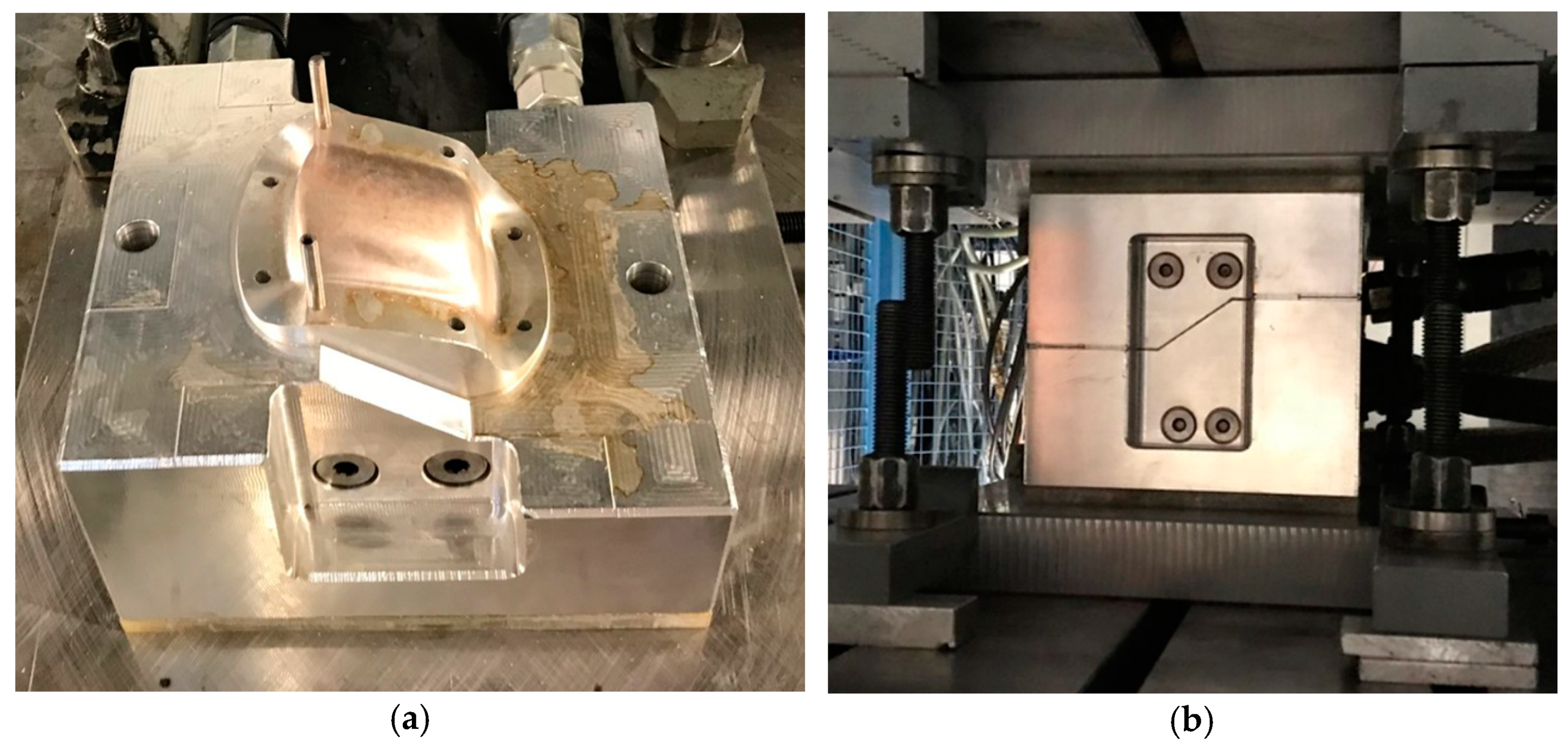
Forming of wood surfaces for a trim part component was performed and the results are compared with simulations. The real forming was carried out in the same way as in the series production process for trim parts. A wooden insert for the palm rest of the Mercedes-Benz X167 series was used. This component is relatively small. Thus, the forming is more dependent on the individual annual ring structure and therefore well suited for model validation. The forming tool is made of aluminum. It consists of a male punch and a female die for forming the topology and two cylindrical pins for fixing the blank, onto which the blank is fitted with holes (Figure 1).
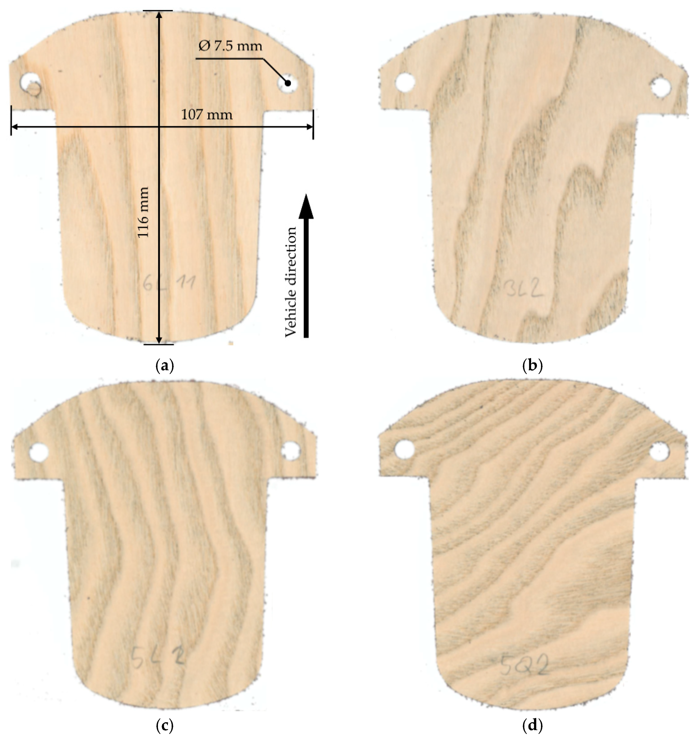
Four different blanks of laminated veneer were used for the experimental and numerical trials. They have the same sample geometry as in the series production process (Figure 2). A CNC-controlled milling machine cut the samples. Ash wood veneers with different textures were used to analyze the influence of the growth ring structure on the forming result. This range corresponds to veneer samples such as those used typically in Mercedes-Benz vehicles. The grain direction was aligned parallel to the length direction of the vehicle for three specimens (Figure 2a–c), as this represents the more critical case. Additionally, the grain direction of one specimen was aligned perpendicularly (Figure 2d).
Samples were put into water at 20 °C for 1 h in order to generate a defined moisture content, as proposed before by Zerbst et al. [2]. The samples achieved a moisture content of around 52%, as determined by the specific weight of a tensile sample after water immersion and oven drying. The forming tool was heated to a constant temperature of 140 °C, as was also carried out in the series production process. The blanks were then placed on the locating pins. The punch was moved at high speed to a distance of 10 mm from the female die. By closing the forming tool at a constant speed of 1 mm/s, the blank was formed and a 3D wooden shell was created under deformation and plasticizing influence of moisture and heat [22].
2.3. Virtual Forming Process
2.3.1. The Digital Twin of the Blank
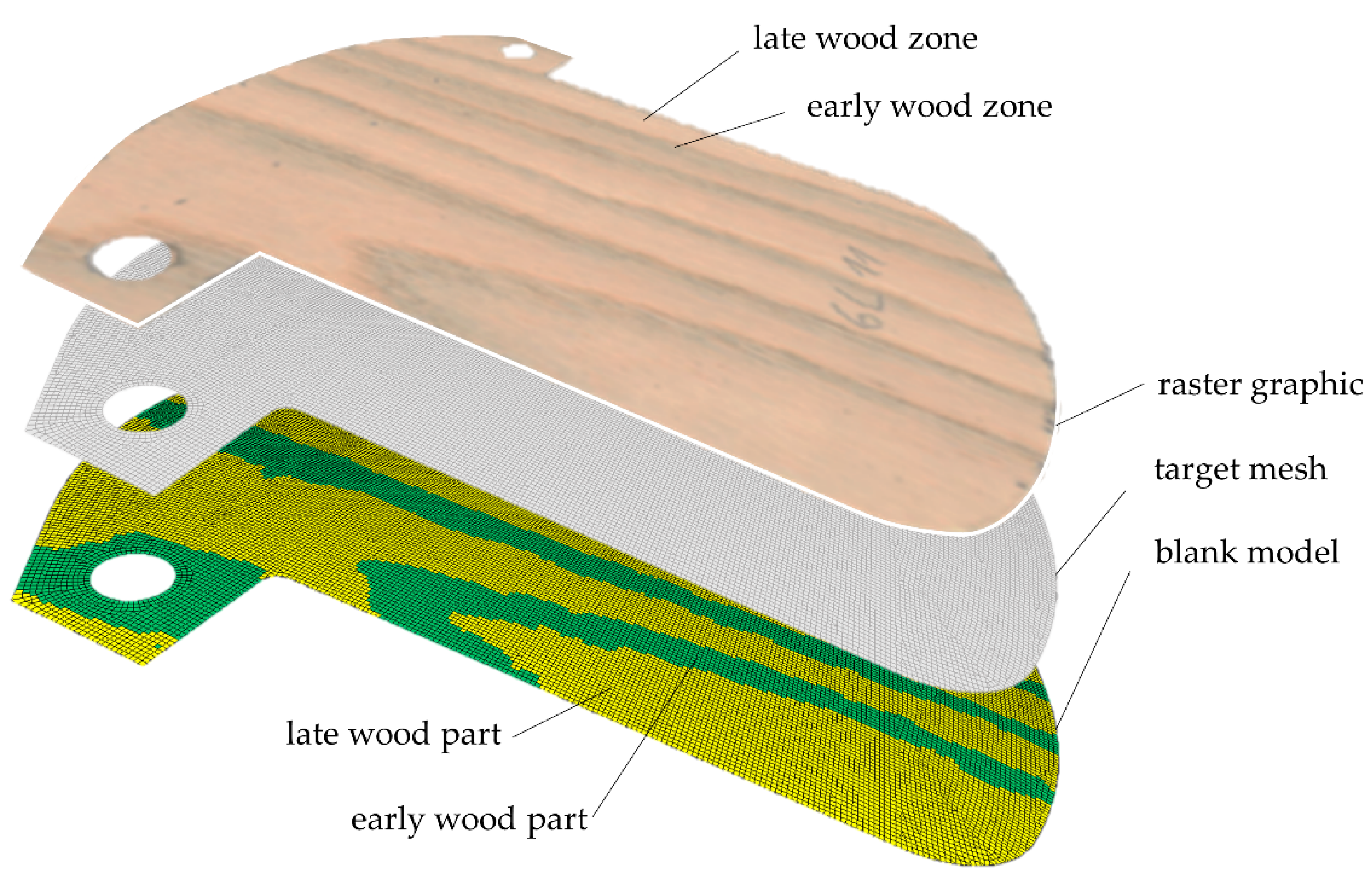
A method for a virtual forming process was developed. Finite element (FE) models of the blank samples used in the experimental forming were created. A gray scale mapping scheme as described by Zerbst et al. [2] was implemented in the mapping software Envyo®. It accounts for early wood (EW) and late wood (LW) areas in the veneer and transfers them to the finite element model. The blank samples, depicted in Figure 2, were scanned individually with a conventional flatbed scanner, resulting in a colored image of each structure. Using the image manipulation program GIMP, the picture was transformed to a gray scale image and exported as ASCII-based portable gray map (pgm) with gray scale values between 0 (completely black) and 255 (completely white) for each pixel. To avoid the transfer of single peaks or artefacts, a Gaussian filter was used to flatten the gray scale values of the picture. As a target for the mapping procedure, an FE model of mainly fully integrated quadrilateral shell elements was created, assuming plane stress for the small ratio of thickness to length of the selected component. The chosen element length of 0.5 mm led to a total number of 34,591 elements for the blank model. After aligning source pixel mesh and target finite element mesh, a nearest neighbor search assigned the corresponding gray scale values to the target elements. In a second step, the elements are assigned to parts in the FE software LS-Dyna that correspond to EW and LW material models (see Figure 3). To obtain consistent results, the gray scale range used to assign EW and LW zones was adjusted for each specimen in a way that a measured width of the EW zones corresponded to the width assigned as EW zone in the finite element mesh. The parameters found for the four specimens used for evaluation purposes of the method are given in Table 1.
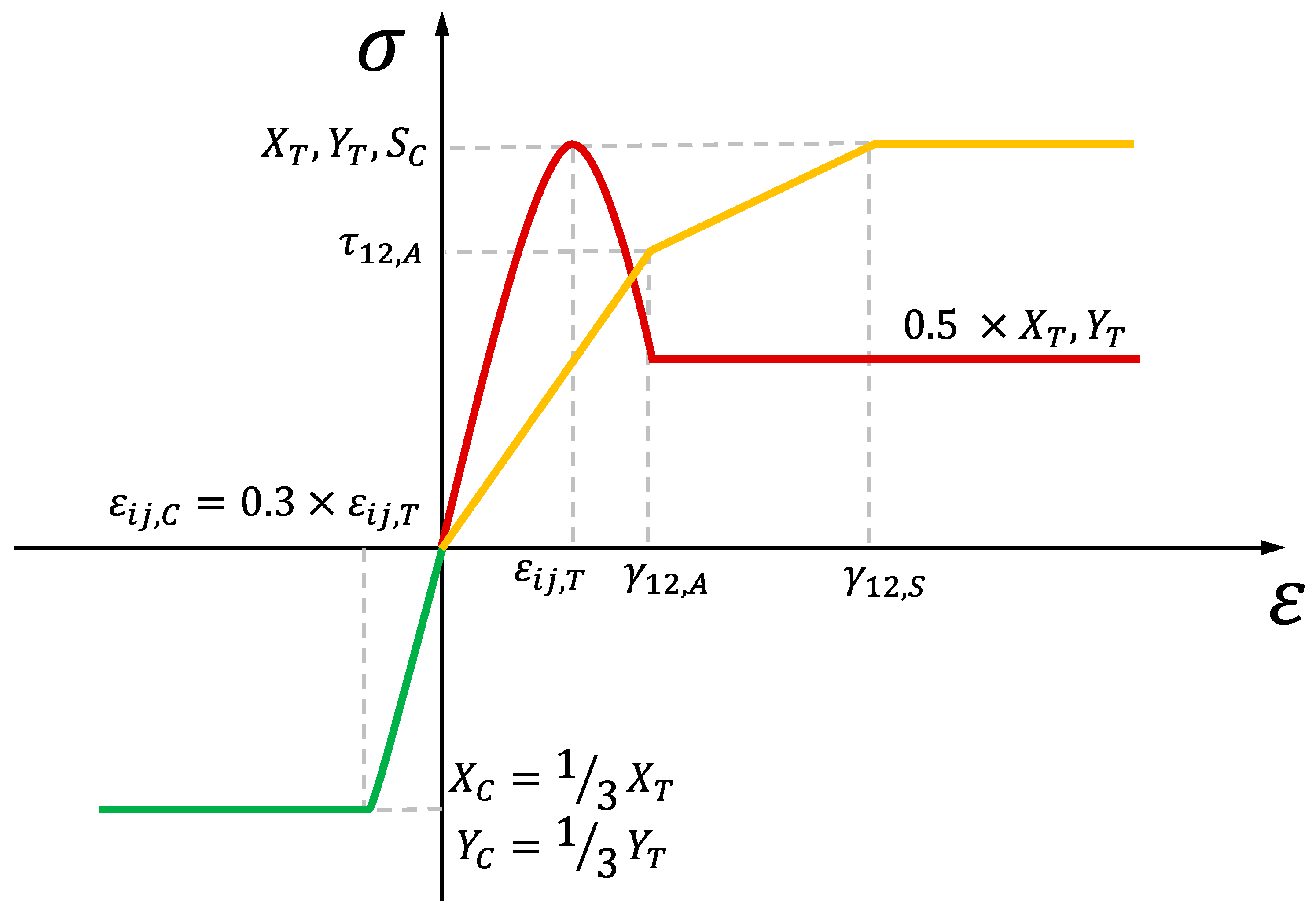
Considering the global mechanical behavior of the laminate, a material model with the name *MAT_LAMINATED_COMPOSITE_FABRIC (*MAT_058) implemented in the FE software LS-DYNA was chosen (Figure 4). *MAT_058 is commonly used to model the transversally anisotropic behavior of laminated composite fabrics [23,24,25] but has been used by for other procedures due to its capability to describe the non-symmetric tension/compression behavior of wood [26]. The advantage of *MAT_058 opposed to other material models is the possibility to consider a non-linear stress–strain relationship under tension and shear. This depicts the behavior of veneer laminates very well, as was shown in our previous paper [1].
The implementation described by Schweizerhof et al. [23] is based on the work proposed by Matzenmiller et al. [27]. In order to reduce efforts for material testing and FE modeling, the material was characterized as a single laminate, avoiding the separate considerations of the single layers. In general, the laminate behavior with respect to stiffness and strength was dominated by the veneer sheet, as stated by Zerbst et al. [2]. For the veneer laminate, material failure was identified for the directions parallel (X) and transverse to the grain orientation (Y), with a maximum stress criterion, under tensile (Index T) or compressive loading (Index C) or under in-plane shear loading (). As described by Zerbst et al. [1], those failure criteria were calibrated for EW and LW material through reverse-engineering, using the optimization software LS-OPT. For the adjustment of the non-linear curve fitting, Young’s moduli () and maximum strains () were identified under tensile loading for the longitudinal (1) and the transverse (2) material directions. Material parameters are provided in Table 2.
Picture frame tests of Zerbst et al. [2] were used to calibrate material behavior under shear loading conditions. The derived parameters for failure (, ) under pure in-plane shearing conditions and the corresponding input values for the stress–strain curve (, , ) are provided in Table 3.
Since testing and measuring of material behavior under compression is challenging due to the tendency of the laminar structure to buckle out of the loading plane, these parameters were derived from literature data. Based on measurements of tension and compression behavior of ash wood and beech wood of Niemz and Sonderegger [28] and Ozyhar et al. [29], compressive failure parameters were derived as provided in Table 4, assuming the same ratio of tension to compression strength and maximum strain. Thereby, the tension–compression strength ratio was chosen as 3:1 parallel to the fiber direction and 1.5:1 perpendicular to the fiber direction for EW:LW. Strain values for maximum strain were reduced by 30% with respect to the tensile loading direction.
In order to account for the remaining stresses after reaching the maximum stress limit prior to element erosion due to maximum strain, *MAT_58 provided the SLIMi values that allow this minimum stress to be defined depending on the loading direction. In this work, stresses were reduced to 50% of the maximum stress in the tensile direction and were kept at the maximum stress level for in-plane shear and compressive direction, as illustrated in Figure 4. The initial main material orientation was assigned using the AOPT—flag equal to 2, allowing for a direction definition in the global coordinate system. The global x-direction (samples 1-3) or y-direction (sample 4) was chosen, which are parallel or transverse to the vehicle travel direction (see Figure 2), respectively. To consider the non-linear shearing behavior, the failure surface flag FS was set equal to −1. Other parameters not listed here were left undefined or were implemented as default values, respectively.
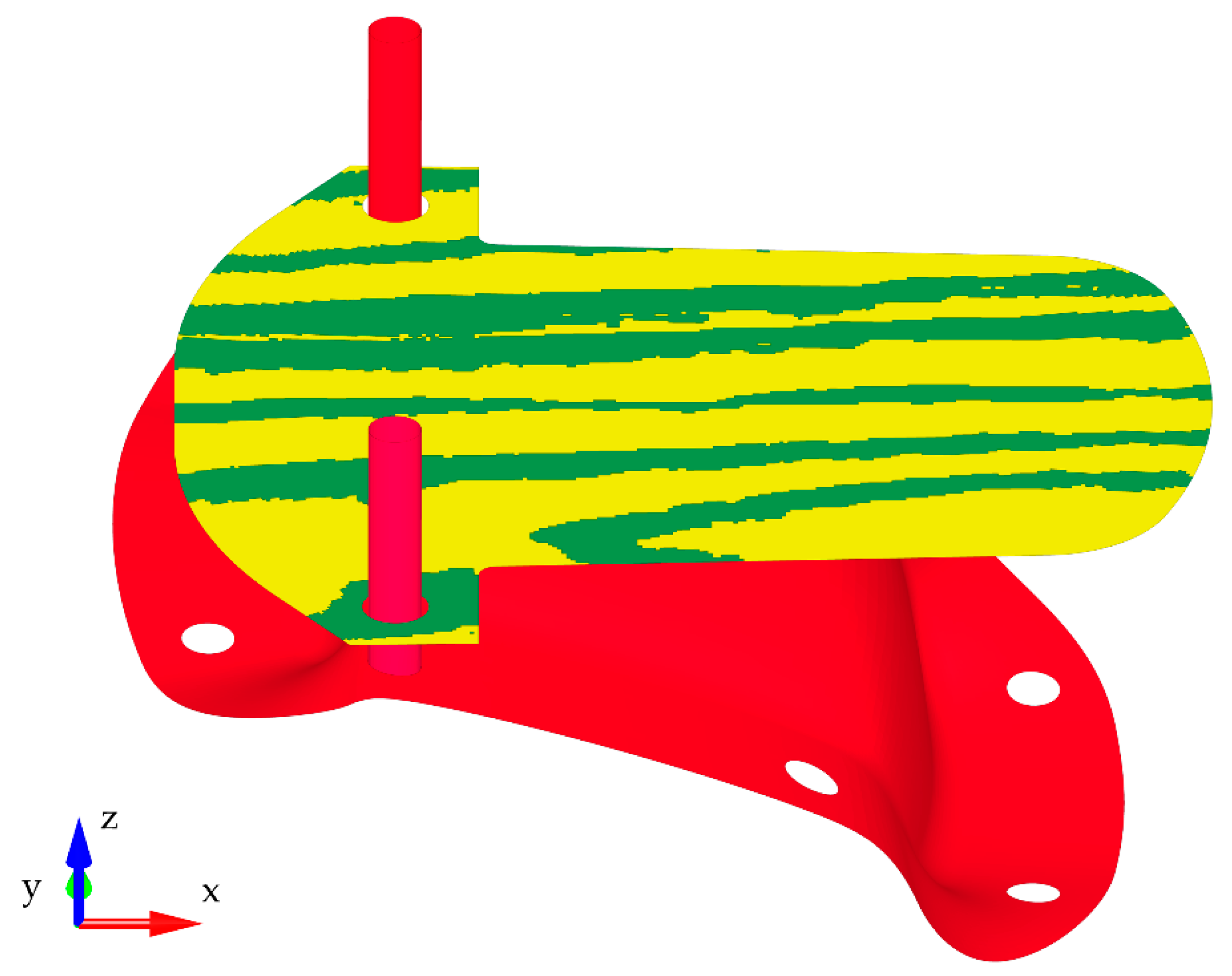
2.3.2. Simulation Step 1: Initial Conditions
This first simulation step accounts for the initial position of the wood component due to gravity loading. The static implicit analysis solution scheme was chosen in order to save calculation time, neglecting inertia and oscillation effects. Due to the expected small displacement of the specimen and a low bending degree, this is a valid approach. As shown in Figure 5, the specimen was placed in the XY plane of the global coordinate system above the die, which is modeled as a rigid body. A total of 43,355 shell elements were used. The gravity loading was applied to the blank part nodes. Segment-based contact algorithms were used between the guiding pens and the specimen. Standard two-way contacts were used between the tool and the specimen. For all contact definitions, a friction coefficient of 0.15 was assumed, based on literature values from measurements of friction between steel surfaces and different wood species at low velocities [30]. The overall time considered in the simulation is 1.5 s. All simulations have been performed on a Linux-based x86 cluster, using 96 parallel CPUs with 5 Gb RAM for both simulation steps. The results presented have been obtained using LS-DYNA-version R11.1 double precision. Within the used environment, a simulation time of about 1 h and 20 min was needed to run this first step of the process simulation.
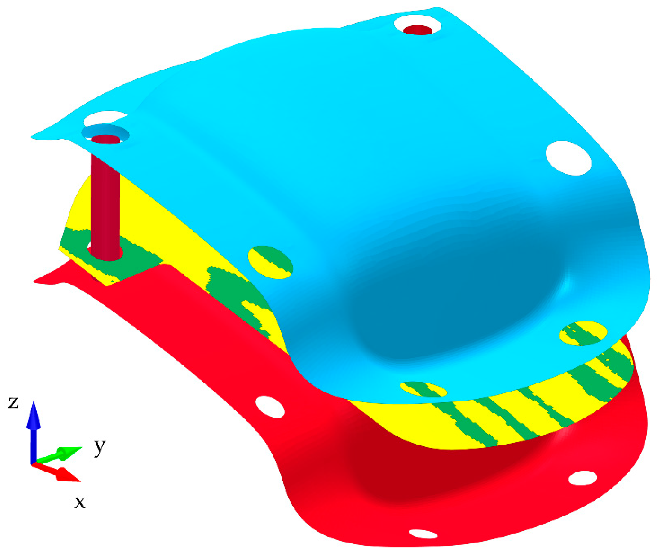
2.3.3. Simulation Step 2: Forming
In the second step, the forming simulation was performed using the estimated initial position from simulation step 1. To do so, the rigid punch model was included (Figure 6). The contact between the guiding pens and specimen was changed to a standard penetration check for nodes to a surface, whereas the contact between the specimen and the tools stayed the same. The simulation was driven by the displacement of the stamping tool, which is supposed to travel 31 mm. The specimen was expected to generate wrinkles, which would lead to instabilities when considering self-contact of the specimen. Therefore, penetrations of the wood specimen were tolerated to allow the stamping tool to travel the full length without creating unphysically high contact forces. Since the method described should allow the detection of wrinkles and not the exact alignment of wood fibers during the forming processes, neglecting the self-contact does not contradict this task.
A total time of 0.1 s was considered in the simulation, which is a 31-fold increase, compared to the true forming velocity, using the explicit solution algorithm with single precision. In the environment described above, the total simulation time was between 8 and 10 min.
3. Results
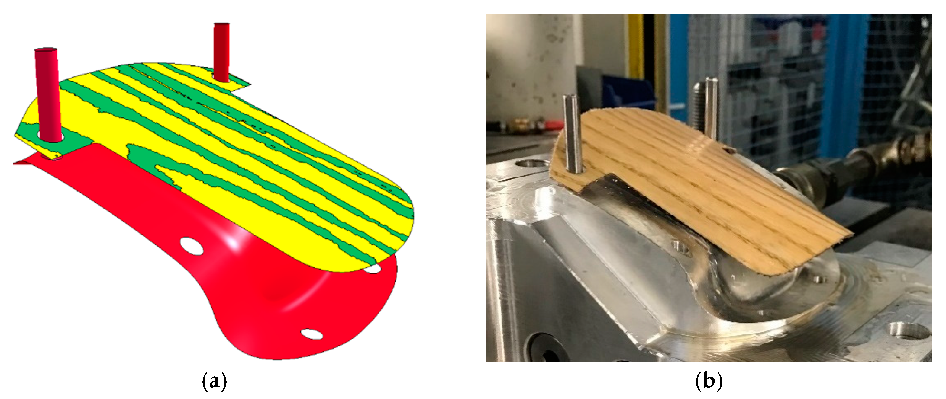
For a validation of the used methods with respect to the quality of the transformation of the true process into a virtual process, experimental and numerical results were compared. Under gravity loading in the first step of the virtual forming process, the blank shifts with the cantilever sight towards the die and slides with a transient oscillation moves into the balance position. The balance position of the simulations (Figure 7a) was the same as observed for the forming experiments (Figure 7b), where the blank was placed by hand. Due to the different swelling behaviors of the veneer and the non-woven layer in consequence of the water pretreatment, the real samples had a curvature from the beginning. This was not considered in the simulation model. However, the gravity simulation provided a good approximation of the initial blank position before the forming started. The determination of the starting conditions of the forming process becomes even more important for larger pieces of trim part surfaces. Those veneer laminate blanks would bend much more in its lying position on the die topology. The effect of a curvature due to the water pretreatment is expected to be lower.
The simulation of the forming process enables the observation of the forming history during the moving punch. This allows analysis of the development of critical deformations (Figure 8). Due to the convex geometry, there is tendency of material compression within the chosen part. Those compressive loads can either be distributed over the sample or localize into buckling and wrinkling modes, depending on the arrangement of the growth rings and the grain orientation. Consequently, the main critical areas are at the circumferential edges.
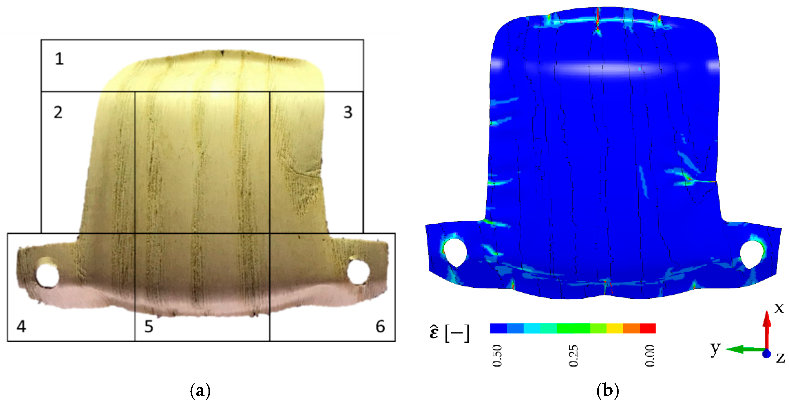
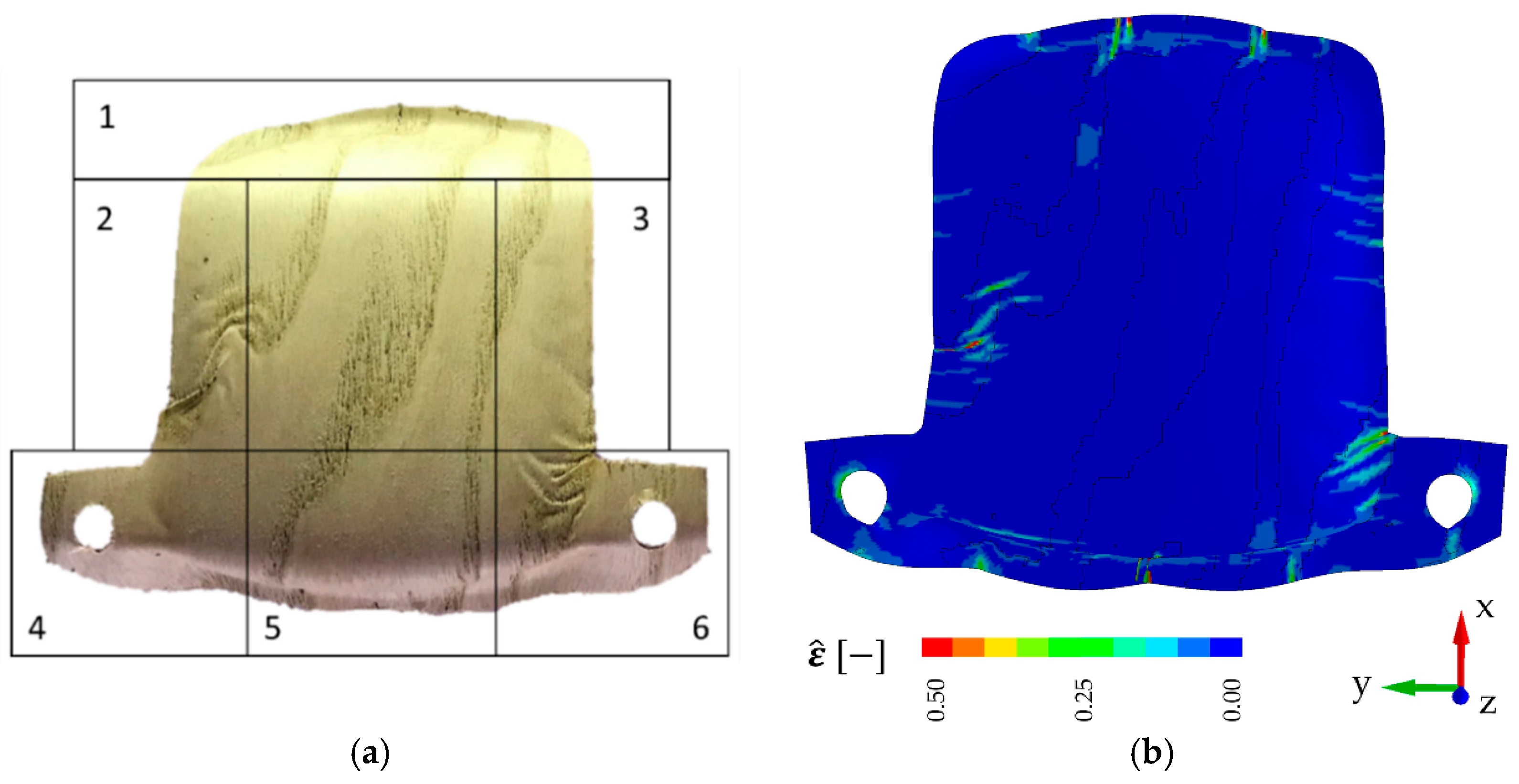
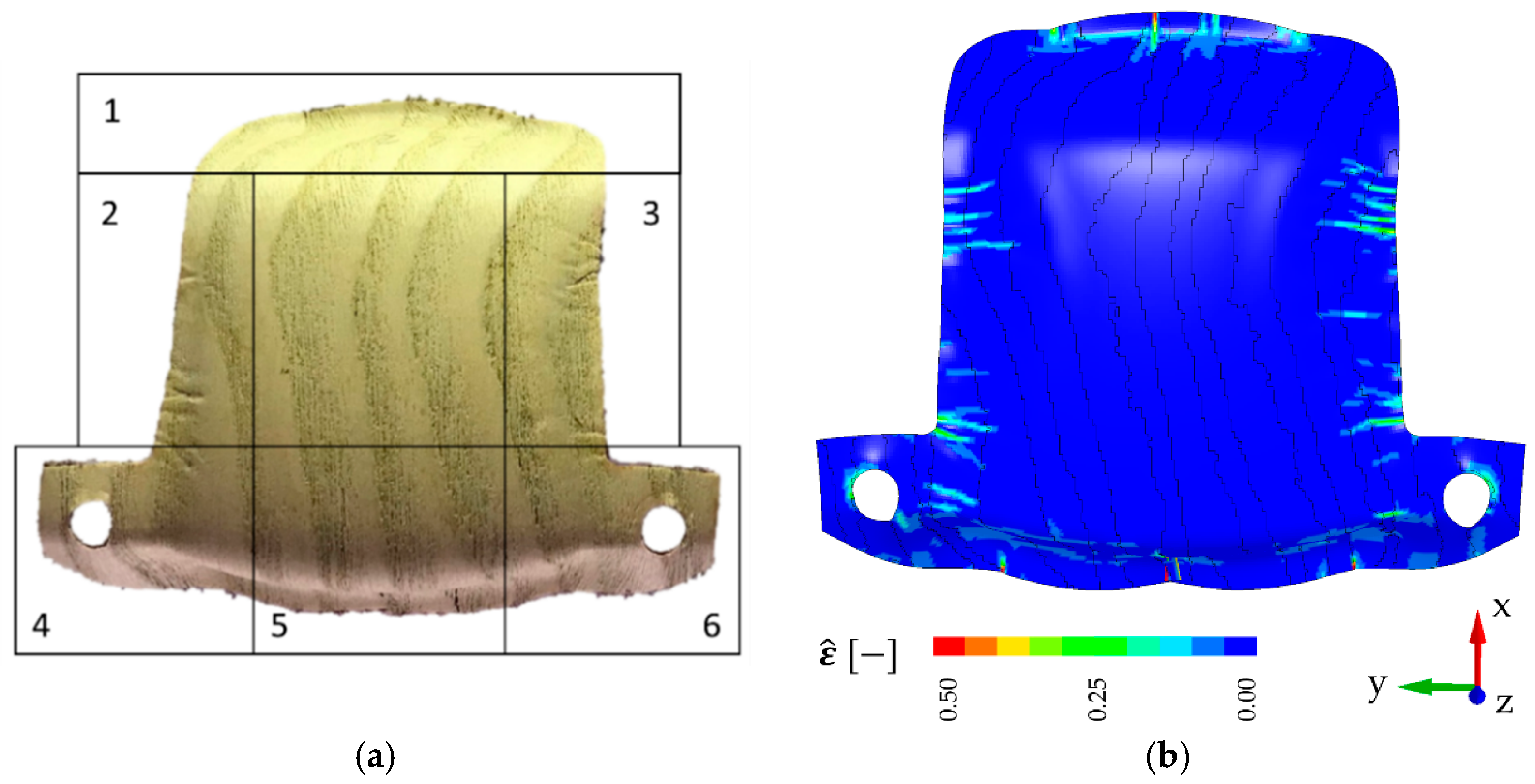
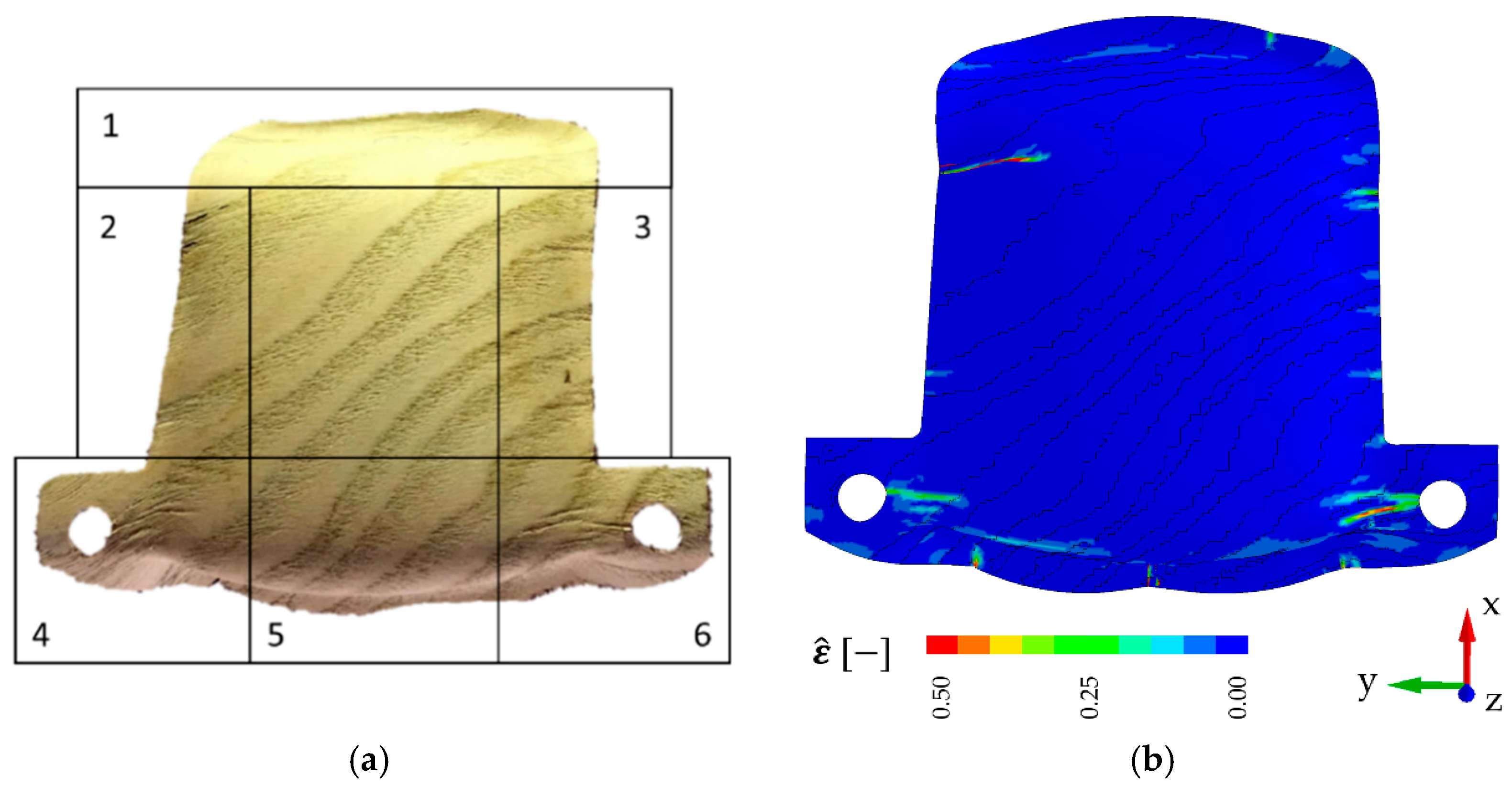
The experimental and numerical forming results are compared below. Characteristic damage phenomena are identified within six zones on the top view images of the physically formed samples (Figure 9a, Figure 10a, Figure 11a and Figure 12a). For further visualization of critical deformations, the simulation results are given in terms of effective strain (Figure 9b, Figure 10b, Figure 11b and Figure 12b). The effective direction of strains as well as their compression or tensile origin is smeared within this scalar measure, with the following equation:
In general, the numerical results provide a very good agreement with the experimental results. The characteristic deformation was captured for all samples with the orientation of the grain direction being parallel as well as perpendicular to the vehicle direction. Corresponding with the specific wood structure, all physical samples and their discrete finite-element representations show buckling and wrinkling behavior, which is mainly induced through the early wood zones. Here, the surrounding stiffer late wood zones thrust the weaker early wood zone. If the geometrical arrangement of the early wood zones is unfavorable, this leads to out-of-plane movement. For early wood zones with higher width, this results into the development of wrinkles, as can be seen in samples and (Figure 9 and Figure 10) in the zones 2 and 3. The constitution of sample , with early wood zones of smaller and uniform width, results in slender compression lines due to forming (Figure 11). The buckling around the pin holes (zones 4 and 6) is also depicted very well by the FE models of samples , and (Figure 9, Figure 10 and Figure 11).
For the orientation of the grain direction perpendicular to the vehicle direction of sample , the simulation shows a larger wrinkle in zone number 3 as well as compression lines running from the pin holes (zones 5 and 6). This is in accordance with the experiment (Figure 12). Some damage is hard to see on the images of the physically formed samples, especially if compression lines developed parallel to the grain direction (Figure 9, Figure 10 and Figure 11 zones 1 and 5, Figure 12, zones 2 and 3). Consequently, such failure is evaluated to be less critical for the assessment of a stable forming process under esthetic criteria.
A larger wrinkle occurred in the middle of zone number 5 for the simulations of all samples. In the experimental forming process, this wrinkle was smaller and not always concentrated to just one early wood zone, as opposed to model predictions. It has to be noted that the parameters of the material models were calibrated in the experiments after water immersion. In the forming process, increased temperature of the tools was used, which generated additional straining capacity due to the softening of wood cell wall components [31,32,33,34,35]. Thus, it was assumed that the simulations represent a more critical case with respect to the material formability. However, the simulations with the proposed modeling process captured the forming behavior of individual wood surfaces accurately.
4. Conclusions
In the present study, veneer sheets were formed physically and numerically into an automotive trim part geometry. Digital twins of the natural samples were created by the gray scale mapping method. The initial position of the blank sheets was considered with a gravity simulation in a good approximation. This first step of the virtual forming process is more important for larger parts, where higher bending over the die is expected. The two-step forming simulation depicted the deformation behavior of each sample with very high accuracy. These results clearly showed that the structural differences between early and late wood and their distribution over the blank sheet are the critical factors for the prediction of the forming behavior of ash wood veneer surfaces. The presented virtual forming process together with the introduced material modelling approach can be used for the development of a stable design of manufacturing processes of veneer forming. Optimizations of the fixation concept or adaptions of the geometry of the tools can be derived based on these simulations. Furthermore, the natural variation of veneer surface composites can be analyzed to make suggestions for the improvement of the material design, e.g., by modifications of the supporting layer of the non-woven backing.
The forming simulation was validated with ring porous ash wood veneer laminate. Apart from that, the virtual process chain can be used for structural-mechanical analysis of many other wood species and applications. High structural density variations due to the season-dependent growth of the tree can also be found for softwood species such as spruce and pine. These species are frequently used in civil engineering, where numerical methods are in high demand for the design of timber structures [36]. These methods can also help to analyze individual conditions in existing constructions.
Author Contributions
Conceptualization, D.Z. and S.C.; methodology, D.Z. and C.L.; software, C.L.; validation, D.Z.; formal analysis, D.Z.; investigation, D.Z.; writing—original draft preparation, D.Z., C.L. and T.G.; writing—review and editing, S.C., T.G. and C.C.; supervision, S.C., T.G. and C.C. All authors have read and agreed to the published version of the manuscript.
Funding
This research received no external funding.
Conflicts of Interest
The authors declare no conflict of interest.
References
- Zerbst, D.; Liebold, C.; Gereke, T.; Haufe, A.; Clauß, S.; Cherif, C. Modelling Inhomogeneity of Veneer Laminates with a Finite Element Mapping Method Based on Arbitrary Grayscale Images. Materials 2020, 13, 2993. [Google Scholar] [CrossRef] [PubMed]
- Zerbst, D.; Affronti, E.; Gereke, T.; Buchelt, B.; Clauß, S.; Merklein, M.; Cherif, C. Experimental analysis of the forming behavior of ash wood veneer with nonwoven backings. Eur. J. Wood Prod. 2020, 65, 107. [Google Scholar] [CrossRef] [Green Version]
- Ormarsson, S.; Sandberg, D. Numerical simulation of hot-pressed veneer products: Moulding, spring-back and distortion. Wood Mater. Sci. Eng. 2007, 2, 130–137. [Google Scholar] [CrossRef]
- Cramer, S.; Kretschmann, D.; Lakes, R.; Schmidt, T. Earlywood and latewood elastic properties in loblolly pine. Holzforschung 2005, 59, 531–538. [Google Scholar] [CrossRef]
- Jernkvist, L.O.; Thuvander, F. Experimental Determination of Stiffness Variation Across Growth Rings in Picea abies. Holzforschung 2001, 55, 309–317. [Google Scholar] [CrossRef]
- Wang, D.; Lin, L.; Fu, F.; Fan, M. Fracture mechanisms of softwood under longitudinal tensile load at the cell wall scale. Holzforschung 2020, 74, 715–724. [Google Scholar] [CrossRef]
- Eder, M.; Jungnikl, K.; Burgert, I. A close-up view of wood structure and properties across a growth ring of Norway spruce (Picea abies [L] Karst.). Trees 2009, 23, 79–84. [Google Scholar] [CrossRef] [Green Version]
- Mott, L.; Groom, L.; Shaler, S. Mechanical properties of individual southern pine fibers. Part II. Comparison of earlywood and latewood fibers with respect to tree height and juvenility. Wood Fiber Sci. 2007, 34, 221–237. [Google Scholar]
- Jenkel, C.; Leichsenring, F.; Graf, W.; Kaliske, M. Stochastic modelling of uncertainty in timber engineering. Eng. Struct. 2015, 99, 296–310. [Google Scholar] [CrossRef]
- Leichsenring, F.; Jenkel, C.; Graf, W.; Kaliske, M. Numerical simulation of wooden structures with polymorphic uncertainty in material properties. IJRS 2018, 12, 24. [Google Scholar] [CrossRef]
- Füssl, J.; Kandler, G.; Eberhardsteiner, J. Application of stochastic finite element approaches to wood-based products. Arch. Appl. Mech. 2016, 86, 89–110. [Google Scholar] [CrossRef]
- Schietzold, F.N.; Graf, W.; Kaliske, M. Polymorphic Uncertainty Modeling for Optimization of Timber Structures. Proc. Appl. Math. Mech. 2018, 18. [Google Scholar] [CrossRef]
- Lukacevic, M.; Füssl, J.; Lampert, R. Failure mechanisms of clear wood identified at wood cell level by an approach based on the extended finite element method. Eng. Fract. Mech. 2015, 144, 158–175. [Google Scholar] [CrossRef]
- Jenkel, C.; Kaliske, M. Finite element analysis of timber containing branches—An approach to model the grain course and the influence on the structural behaviour. Eng. Struct. 2014, 75, 237–247. [Google Scholar] [CrossRef]
- Lukacevic, M.; Kandler, G.; Hu, M.; Olsson, A.; Füssl, J. A 3D model for knots and related fiber deviations in sawn timber for prediction of mechanical properties of boards. Mater. Des. 2019, 166, 107617. [Google Scholar] [CrossRef]
- Lukacevic, M.; Füssl, J. Numerical simulation tool for wooden boards with a physically based approach to identify structural failure. Eur. J. Wood Prod. 2014, 72, 497–508. [Google Scholar] [CrossRef]
- Jenkel, C.; Kaliske, M. Simulation of failure in timber with structural inhomogeneities using an automated FE analysis. Comput. Struct. 2018, 207, 19–36. [Google Scholar] [CrossRef]
- Dexle, C.; Wiblishauser, M. Furniersystem hoher Flexibilität und Verfahren zur Herstellung eines solchen. 1998DE-1003262. Eur. J. Wood Wood Prod. 1998, 78, 321–331. [Google Scholar]
- PWG VeneerBackings GmbH. Technisches Datenblatt Rohvlies 90P-RAW; PWG VeneerBackings GmbH: Walkertshofen, Germany, 2017. [Google Scholar]
- Gindl, W.; Schöberl, T.; Jeronimidis, G. The interphase in phenol–formaldehyde and polymeric methylene di-phenyl-di-isocyanate glue lines in wood. Int. J. Adhes. Adhes. 2004, 24, 279–286. [Google Scholar] [CrossRef]
- Konnerth, J.; Gindl, W. Mechanical characterisation of wood-adhesive interphase cell walls by nanoindentation. Holzforschung 2006, 60, 429–433. [Google Scholar] [CrossRef]
- Navi, P.; Sandberg, D. Thermo-Hydro-Mechanical Processing of Wood, 1st ed.; EPFL Press: Lausanne, Switzerland; CRC Press: Lausanne, Switzerland; Boca Raton, FL, USA, 2012; ISBN 9781439860427. [Google Scholar]
- Schweizerhof, K.; Weimar, K.; Münz, T.; Rottner, T. Crashworthiness analysis with enhanced composite material models in LS-DYNA-merits and limits. In Proceedings of the LS-DYNA World Conference, Detroit, MI, USA, 21–22 September 1998; pp. 1–17. [Google Scholar]
- Cherniaev, A.; Montesano, J.; Butcher, C. Modeling the Axial Crush Response of CFRP Tubes using MAT054, MAT058 and MAT262 in LS-DYNA. In Proceedings of the 15th International LS-DYNA Users Conference, Dearborn, MI, USA, 10–12 June 2018. [Google Scholar]
- Coulton, J. Improvements of material 58 (woven composites) (Addition of strain rate effects). In Proceedings of the LS-DYNA Anwender Forum, Stuttgart, Germany, 25 September 2013. [Google Scholar]
- Baumann, G.; Hartmann, S.; Müller, U.; Kurzböck, C.; Feist, F. Comparison of the two material models 58, 143 in LS Dyna for modelling solid birch wood. In Proceedings of the 12th European LS-DYNA Conference, Koblenz, Germany, 14–16 May 2019. [Google Scholar]
- Matzenmiller, A.; Lubliner, J.; Taylor, R.L. A constitutive model for anisotropic damage in fiber-composites. Mech. Mater. 1995, 20, 125–152. [Google Scholar] [CrossRef]
- Niemz, P.; Sonderegger, W.U. Holzphysik: Physik des Holzes und der Holzwerkstoffe; Carl Hanser Verlag GmbH & Company KG: Munich, Germany, 2018; ISBN 9783446457218. [Google Scholar]
- Ozyhar, T.; Hering, S.; Niemz, P. Moisture-dependent orthotropic tension-compression asymmetry of wood. Holzforschung 2013, 67, 395–404. [Google Scholar] [CrossRef] [Green Version]
- McKenzie, W.M.; Karpovich, H. The frictional behaviour of wood. Wood Sci. Technol. 1968, 2, 139–152. [Google Scholar] [CrossRef]
- Back, E.L.; Salmen, N.L. Glass transitions of wood components hold implications for molding and pulping processes. Tappi J. 1982, 65, 107–110. [Google Scholar]
- Goring, D. Thermal softening of lignin, hemicellulose and cellulose. Pulp Pap. Mag. Can 1963, 64, T517–T527. [Google Scholar]
- Hillis, W.E.; Rozsa, A.N. The Softening Temperatures of Wood. Holzforschung 1978, 32, 68–73. [Google Scholar] [CrossRef]
- Irvine, G.M. The glass transitions of lignin and hemicellulose and their measurement by differential thermal analysis. Tappi J. 1984, 67, 118–121. [Google Scholar]
- Börcsök, Z.; Pásztory, Z. The role of lignin in wood working processes using elevated temperatures: An abbreviated literature survey. Eur. J. Wood Prod. 2020. [Google Scholar] [CrossRef]
- Füssl, J.; Lukacevic, M.; Pillwein, S.; Pottmann, H. Computational Mechanical Modelling of Wood—From Microstructural Characteristics Over Wood-Based Products to Advanced Timber Structures. In Digital Wood Design: Innovative Techniques of Representation in Architectural Design; Bianconi, F., Filippucci, M., Eds.; Springer International Publishing: Cham, Switzerland, 2019; pp. 639–673. ISBN 978-3-030-03675-1. [Google Scholar]
Figure 1.
(a) Die with pins for the fixation of the veneer laminate; (b) closed tool in the forming press.
Figure 1.
(a) Die with pins for the fixation of the veneer laminate; (b) closed tool in the forming press.

Figure 2.
Forming samples of different texturing through the ash wood growth rings with numbers: (a) , (b) , (c) , (d) .
Figure 2.
Forming samples of different texturing through the ash wood growth rings with numbers: (a) , (b) , (c) , (d) .

Figure 3.
Schematic view of the generation of digital twins of the blank samples by the gray scale mapping scheme.
Figure 3.
Schematic view of the generation of digital twins of the blank samples by the gray scale mapping scheme.

Figure 4.
General behavior of *MAT_058 in tension (red), compression (green) and shear (yellow) as used for wood modeling in this work.
Figure 4.
General behavior of *MAT_058 in tension (red), compression (green) and shear (yellow) as used for wood modeling in this work.

Figure 5.
FE model of the gravity simulation.

Figure 6.
FE model of the forming simulation.

Figure 7.
(a) Balance position of the blank from the gravity simulation ( = 1.5 s); (b) initial position in the true forming process.
Figure 7.
(a) Balance position of the blank from the gravity simulation ( = 1.5 s); (b) initial position in the true forming process.

Figure 8.
Development of deformations of sample 1 over the time of the closing process of the punch in the simulation.
Figure 8.
Development of deformations of sample 1 over the time of the closing process of the punch in the simulation.

Figure 9.
Forming results of sample . (a) Experiment; (b) simulation with output of equivalent strain.
Figure 9.
Forming results of sample . (a) Experiment; (b) simulation with output of equivalent strain.

Figure 10.
Forming results of sample . (a) Experiment; (b) simulation with output of equivalent strain.
Figure 10.
Forming results of sample . (a) Experiment; (b) simulation with output of equivalent strain.

Figure 11.
Forming results of sample . (a) Experiment; (b) simulation with output of equivalent strain.
Figure 11.
Forming results of sample . (a) Experiment; (b) simulation with output of equivalent strain.

Figure 12.
Forming results of sample . (a) Experiment; (b) simulation with output of equivalent strain.
Figure 12.
Forming results of sample . (a) Experiment; (b) simulation with output of equivalent strain.


Table 1.
Gray scale ranges for the mapping of early wood (EW) and late wood (LW) zones of all samples.
Table 1.
Gray scale ranges for the mapping of early wood (EW) and late wood (LW) zones of all samples.
| Sample No. | Gray Scale Ranges | |
|---|---|---|
| LW | EW | |
| 0–212 | 213–255 | |
| 0–205 | 206–255 | |
| 0–205 | 206–255 | |
| 0–204 | 205–255 | |
Table 2.
Calibrated material parameter in tensile loading direction for EW and LW obtained in [2].
Table 2.
Calibrated material parameter in tensile loading direction for EW and LW obtained in [2].
| Part | ||||||||
|---|---|---|---|---|---|---|---|---|
| (MPa) | (MPa) | (MPa) | (MPa) | (-) | (-) | (-) | (-) | |
| LW | 4452 | 600 | 61 | 27 | 0.039 | 0.116 | 0.42 | 0.05660 |
| EW | 2000 | 136 | 30 | 12 | 0.056 | 0.207 | 0.42 | 0.02751 |
Table 3.
Calibrated material parameter for in-plane shear behavior for EW and LW.
| Part | |||||
|---|---|---|---|---|---|
| (MPa) | (MPa) | (-) | (MPa) | (-) | |
| LW | 800 | 9 | 0.064 | 15 | 0.212 |
| EW | 300 | 7 | 0.15 | 8 | 0.360 |
Table 4.
Estimated material parameters for compressive loading for EW and LW.
| Part | ||||
|---|---|---|---|---|
| (MPa) | (MPa) | (-) | (-) | |
| LW | 24 | 18 | 0.026 | 0.078 |
| EW | 12 | 8 | 0.038 | 0.140 |
Publisher’s Note: MDPI stays neutral with regard to jurisdictional claims in published maps and institutional affiliations. |
© 2021 by the authors. Licensee MDPI, Basel, Switzerland. This article is an open access article distributed under the terms and conditions of the Creative Commons Attribution (CC BY) license (https://creativecommons.org/licenses/by/4.0/).
Share and Cite
MDPI and ACS Style
Zerbst, D.; Liebold, C.; Gereke, T.; Clauß, S.; Cherif, C. Numerical Simulation of the Forming Process of Veneer Laminates. J. Compos. Sci. 2021, 5, 150. https://0-doi-org.brum.beds.ac.uk/10.3390/jcs5060150
AMA Style
Zerbst D, Liebold C, Gereke T, Clauß S, Cherif C. Numerical Simulation of the Forming Process of Veneer Laminates. Journal of Composites Science. 2021; 5(6):150. https://0-doi-org.brum.beds.ac.uk/10.3390/jcs5060150
Chicago/Turabian StyleZerbst, David, Christian Liebold, Thomas Gereke, Sebastian Clauß, and Chokri Cherif. 2021. "Numerical Simulation of the Forming Process of Veneer Laminates" Journal of Composites Science 5, no. 6: 150. https://0-doi-org.brum.beds.ac.uk/10.3390/jcs5060150