Evaluation of ARIMA Models for Human–Machine Interface State Sequence Prediction


1
Computers, Controls and Design Department, Ontario Power Generation, Pickering, ON L1V 2R5, Canada
2
Department of Electrical, Computer and Software Engineering, University of Ontario Institute of Technology, Oshawa, ON L1G 0C5, Canada
*
Author to whom correspondence should be addressed.
Mach. Learn. Knowl. Extr. 2019, 1(1), 287-311; https://0-doi-org.brum.beds.ac.uk/10.3390/make1010018
Submission received: 16 November 2018
/
Revised: 22 December 2018
/
Accepted: 24 December 2018
/
Published: 3 January 2019
(This article belongs to the Section Learning)
Abstract
:In this paper, auto-regressive integrated moving average (ARIMA) time-series data forecast models are evaluated to ascertain their feasibility in predicting human–machine interface (HMI) state transitions, which are modeled as multivariate time-series patterns. Human–machine interface states generally include changes in their visually displayed information brought about due to both process parameter changes and user actions. This approach has wide applications in industrial controls, such as nuclear power plant control rooms and transportation industry, such as aircraft cockpits, etc., to develop non-intrusive real-time monitoring solutions for human operator situational awareness and potentially predicting human-in-the-loop error trend precursors.
1. Introduction
Operator situational awareness (SA) is quintessential in ensuring safe operation of any industrial establishment and more so in nuclear power plants (NPP). Nuclear power plant industrial accidents (rating as per the ascending order of severity scale ranging between 1 (Anomaly) to 7 (Major accident) on the International Atomic Energy Agency’s (IAEA) International Nuclear Event Scale (INES) [1]), include such cases as National Research Reactor (NRX) at Chalk River, Canada (INES-5)—where multiple failures involving incorrect control rod status indicator lights in the control room, mechanical failures, and miscommunication between control room personnel led to the accidental withdrawal of the safeguard bank of shut-off rods, causing an uncontrolled reactor power excursion over four times the reactors design limit in a matter of 5 s, resulting in a severe core damage on 12 December 1952; Three Mile Island, USA (INES-5)—where poorly designed ambiguous control room indicators introduced operator error to override the emergency cooling water supply, causing a partial meltdown of the Three Mile Island Unit-2 (TMI-2) reactor core containment on 28 March 1979; and the Chernobyl accident, USSR (INES-7)—where confounding human factors and inherent design flaws led to a catastrophic reactor Unit 4 explosion and release of radioactivity on 26 April 1986.
Key accident precursors, as evident from the post-accident reports [2,3,4], include: (1) reduction in situational awareness owing to human factor related deficiencies in legacy human–machine interface (HMI design); (2) normalization to deviance to lax nuclear safety culture; (3) information overload (looking-but-not-seeing effects [5]) owing to the rapid rate at which information was presented to operators via the control room HMIs (panel indications, annunciations, etc.); and (4) incorrect mental model of highly dynamic unit evolutions resulting in cognitive errors, owing to conflicting plant information supplied by failed or faulty sensors and incorrect field equipment status monitoring.
In order to address accident precursors, the NPP industry has incorporated frequent training programs covering several accident scenarios in simulation to prepare NPP operators to: (1) mentally filter non-essential information and prioritize responses; (2) validate assumptions; (3) constantly maintain situational awareness; (4) align their mental models with evolving plant process states; and (5) practice strict adherence to operating and alarm response procedures to control an evolving unit transience.
In summary, the NPP industry stands to benefit from solutions targeted to key challenges in areas of (1) non-intrusive real-time monitoring of situational awareness; (2) predicting human error; (3) retrofit legacy HMIs to offer SA monitoring, with the benefit being human errors can either be predicted shortly prior to being introduced or can promptly be intervened upon to avoid minor faults to magnify over time at the expense of delayed response.
To this end, the objective of this research is to develop a non-intrusive operator SA monitoring solution for industrial control room application, to preserve personnel privacy and improve safe operation.
Non-Intrusive Situational Awareness Monitoring
An abstraction of the legacy command–control–feedback control architecture (Figure 1A) exposes a general lack of automatic cross-validation between operator inputs and process states in this view. Most man–machine interfaces seldom incorporate checks to monitor human-in-the-loop errors injected through operator command actions via HMIs. Where, in fact the onus is on operators who must rely on manual effort and acquired cognitive skills to reduce human errors and be self-cognizant of situational awareness. However, while rigorous operator training does minimize human command input errors, in reality, unit transients do continue to fatigue the human mind owing to sensory overload, thus increasing chances of human-in-the-loop cognitive errors.
In contrast, non-intrusive monitoring of operator situational awareness, that may be achieved by various means such as that proposed by the expert supervisory system (EYE)-on-HMI framework [6] (using computer vision), incorporates a closed-loop independent cross-validation over the conventional operator-based command–control–feedback architecture (Figure 1B). Cross-validation, firstly, can be achieved by verifying what the operator is visualizing from the HMI does truly match the plant process state. Under this approach, operator performance is be being tracked indirectly via their interactions with the HMI, which can be interpreted by changes in HMI states, rather than directly monitoring operator gestures and actions. Secondly, logging and verifying whether operator command input patterns in response to the current HMI state is in fact safe and in alignment with the approved procedure(s) can aid in monitoring operator situational awareness in real-time.
The proposed approach is to treat HMI states as time-series (TS) data that can be used to train an Auto-Regressive Integrated Moving Average (ARIMA) model. The ARIMA model has seen wide use in forecasting time-series data. A novel application of this statistical tool is to detect deviation in normal sequence of events shown by physical HMI devices such as indication lights, displays, meters, alarm windows, etc. via non-intrusive means [7]. Sequence deviations can then be trended and used as a measure for operator situational awareness. In certain scenarios the time-series forecast models can also predict particular human errors prior to occurring based on historical trends.
The rest of the paper is organized as follows: Section 2 presents a review of current state-of-the-art relevant to proposed time-series data forecasting and its applications. Section 3 introduces the model, and Section 4 outlines the methodology for experiment setup, data preparation, and model building approach. Section 5 discusses the experimental results and ARIMA model limitations. Finally, Section 6 concludes the paper and offers ideas for future work.
2. Related Work
In order to ensure operator SA does not deteriorate while using HMIs (e.g., control panels, cockpits information display designs, etc.), careful assessment and incorporation of human factor design elements in engineered systems is required. Therefore, the NPP industry currently has a niche for an online system to monitor operator SA that warns by predicting adverse human performance trends in real-time.
Several works have addressed modelling human-in-the-loop (HITL) errors or estimating human error probabilities (HEPs). For instance, notably, the legacy human reliability analysis (HRA) [8,9] approach has been re-hauled (e.g., the first and second generation models [10]) since its first introduction in the 1950s [11]. Human reliability analysis is concerned with qualitatively and quantitatively estimating human contribution to risk and has also been adopted in probabilistic risk assessment for critical nuclear power plant systems.
Work such as Reference [11] use Bayesian belief networks and incorporate performance shaping factors (PSFs) [12,13] to improve predicting HEPs relevant to particular industrial task. Performance shaping factors annotate various aspects of the context (or environment) (e.g., HMI design parameters, etc.) and human behavior (e.g., situational awareness) that can impact human performance. For instance, PSF is shown to set the operator context, which ultimately affects HEP. Reference [14] showed a linear regression model built using a work condition parameter surveys database that could then be used to predict certain human error omens (precursors) based on routine personnel surveys done in NPPs. The particular underlying challenge in previous approaches has remained with adequately capturing a causal relationship between HEPs and PSF.
However, since the HRA approach incorporates behavioral science and cognitive psychology, with plant process states and various first- and second-generation HRA methodologies [15], there is less emphasis on non-intrusive monitoring and prediction of HITL errors in real-time.
As previously stated, this paper treats HMI states as time-series (TS) data to realize a non-intrusive means of estimating operator error compared to normal HMI state patterns. The parallels of this specific problem can be found in other research domains such as in autonomous vehicles [16,17], weather patterns [18], and stock price index prediction [19,20], etc. Such approaches involve relying on the underlying multi-physics and variable dynamic models, which are infused with sensor or process noise estimation techniques such as unscented Kalman filters [16] (for non-linear estimation). Evidently, the process model-based prediction techniques require process domain specific knowledge and may not scale well as the number of system/process variables increase. Other prevalent prediction approach is a rather black-box approach where only sparse knowledge of the underlying process is required. Works such as Reference [21] employ deep convolutional neural networks (CNNs) for computer vision data processing to mimic human visual cognition for object identification and classification. Similar to this later approach, we adopt the black-box modeling of HMI state patterns. This shall scale well to model multi-variate TS for arbitrary HMI display systems.
Time-series data forecast modeling is a vast area of research employing varied techniques ranging from linear statistical models to non-linear recurrent neural networks. Nevertheless, under the current scope only works that use linear stochastic models using the ARIMA model is being investigated owing to their simplicity and deterministic behavior. The ARIMA model allows training forecast models using statistical means to capture standard temporal structures in time-series data.
The ARIMA or Box–Jenkins method was first introduced in 1970s [22]. It has seen numerous applications in various areas for forecasting processes such as stock prices [23], electricity market [24], computer hardware resource [25,26], natural phenomena [27], etc., that yield time-series data. In Reference [26], ARIMA and long short-term memory (LSTM) recurrent network for forecasting performance of CPU (Central Processing Unit) usage of server machines in data centers are compared. They showed that ARIMA does not quite model non-linear temporal relationships where the CPU data is unstable and volatile requiring high effort in data transformation to build a functional model. A hybrid approach combining ARIMA and wavelet decomposition approach is proposed in Reference [25] to accurately predict the number of arriving tasks to a cloud data center at the next time interval.
3. HMI Model
3.1. HMI State Space Model
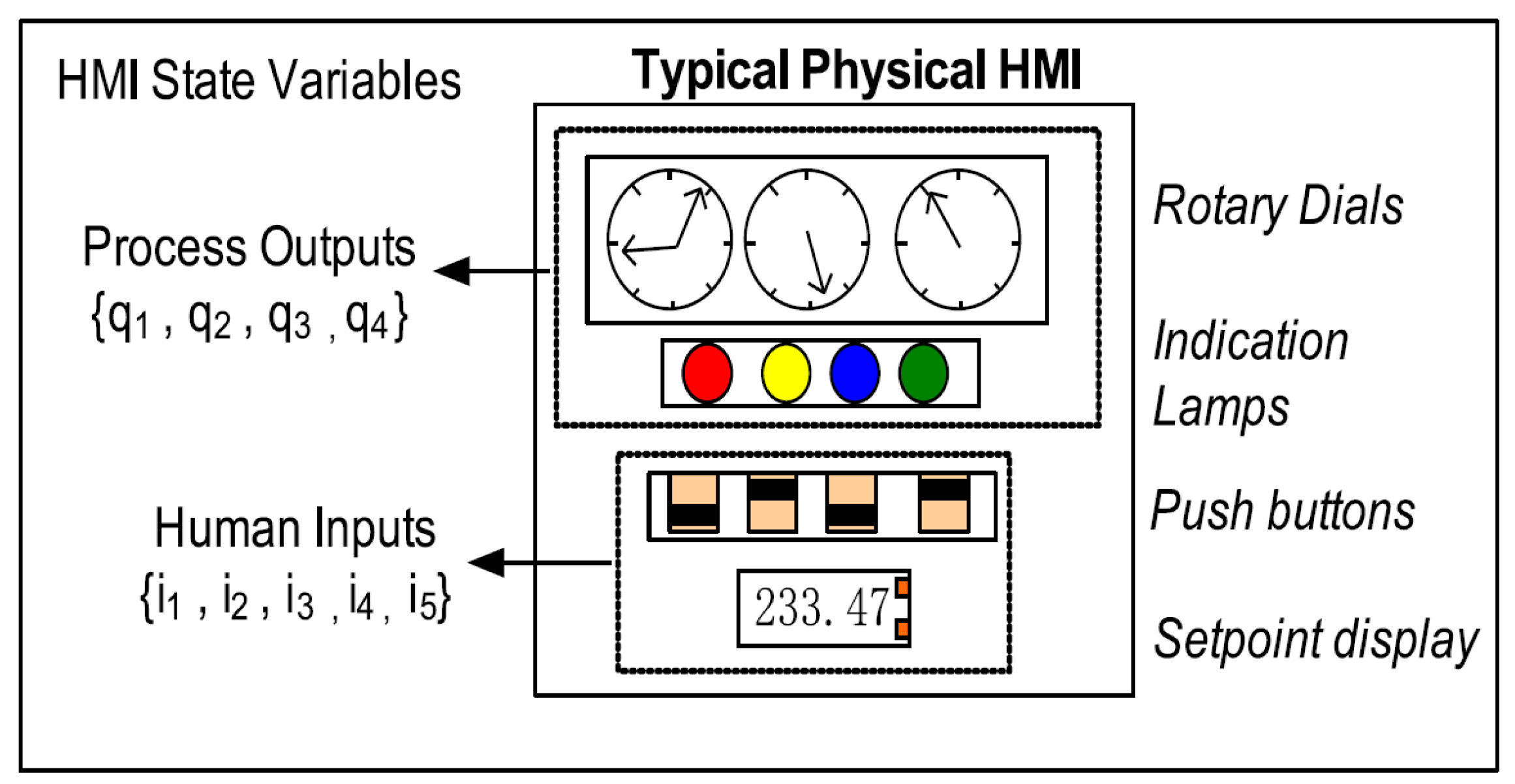
Conceptually, HMI states (Figure 2) of any given process can sufficiently be captured by two categories of state variables: process outputs and human inputs. Each variable can take on either binary values (e.g., indication lamp states, push buttons states, etc.) or a finite range of analogue values (e.g., rotary dial indicators, digital setpoint displays, etc.). For example, in Figure 2, process outputs q1, q2, and q3 are analogue variables that can be associated with each rotary dial value, and q4, an integer variable, can capture various lamp indication patterns. Human user inputs i1, i2, i3, and i4 are digital variables that can be associated with each push button, and i5, analogue variable, can be associated with a setpoint indicator. An ensemble of all these multi-data type variables (or features) can sufficiently capture all states of the HMI. Logging these HMI states yields multi-variate time-series data.
3.2. HMI State Time-Series (TS)
A series of data points that are indexed at equal time intervals is referred to as time-series data. Uni-variate or multi-variate time-series (TS) data captures the sequences with-in processes such that the next time step state data is dependent on the process state at previous time steps. Time-series analysis differs from classical classification and regression predictive modelling, in that the temporal structure that envelopes underlying patterns must be captured. For example, weather data, stock prices, industrial processes, etc. Analysis of time-series data attempts to extract and model such dependencies which can then be used to do n-steps ahead forecast of the process state variables.
3.3. Weakly Stationary Assumptions
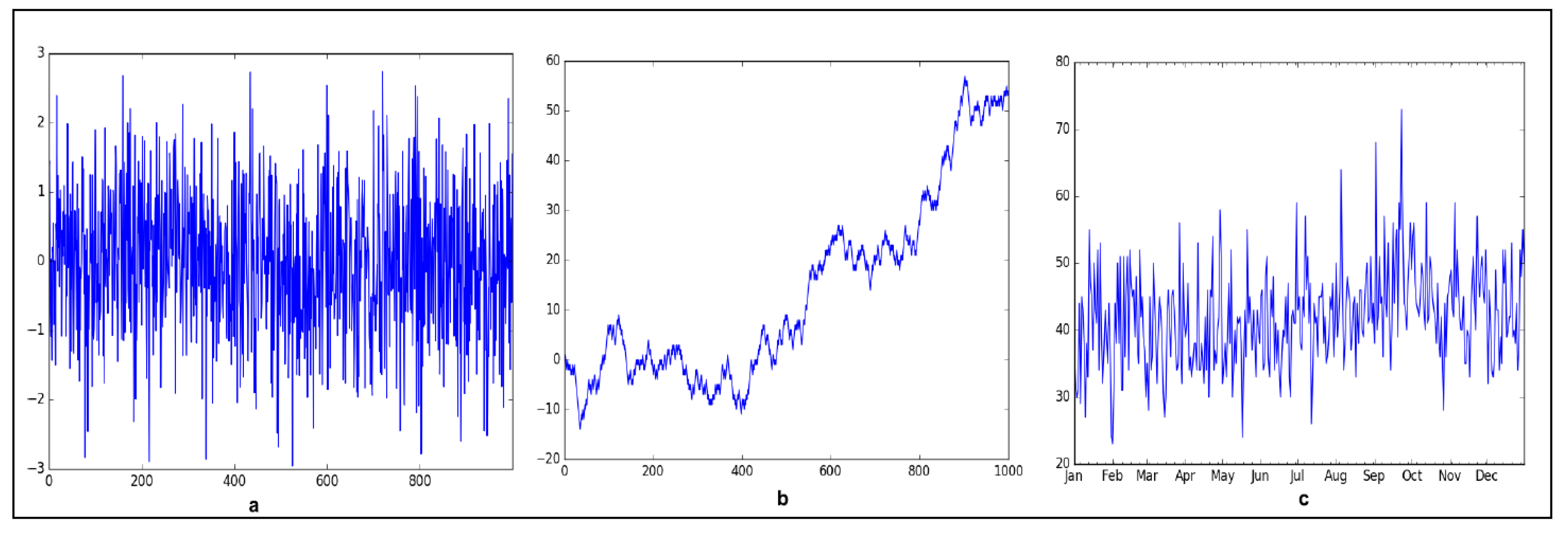
Few plausible and helpful assumptions for HMI state patterns are rationalized below: Firstly, a HMI process cannot yield a data series that is white noise (ε) (Figure 3a)—a series that is generated by random variables that are independent and identically distributed, i.e., having zero mean (μ = 0), with identical finite variance (σ2) < ∞ that are serially uncorrelated E[εtεk] for all t ≠ k (Equation (1)).
A white noise (Figure 3a) TS is statistically random, unpredictable, and thus cannot be modelled for practical purposes. However, we ideally expect the HMI state time-series forecast errors or residuals to be white noise, which implies there are no recoverable patterns left to be learned from the forecast errors (difference between actual and predicted value output by the forecast model). An HMI displaying white noise state patterns would suggest an error or malfunction in the process.
Second assumption, is that a majority of HMI state transition can be modelled as stochastic processes that yield a weakly stationary multi-variate time-series in most practical scenarios. A weakly stationary process must satisfy three conditions as listed in Equation (2) and yields a TS (Figure 3c) of values whose mean (1) (μ < ∞) (2) variance (σ2 < ∞) are finite and constants for all t windows (i.e., these do not vary with time), while (3) the auto-covariance (γ(t, k)) between any observed values at two time slices of a stochastic process is finite and constant for all τ, that is, the auto-covariance of a weakly stationary TS only depends on the temporal distance (τ = |t − k|) between any two time points (t and k), as shown in Figure 4. Auto-covariance when normalized by standard deviation of each observation of TS, results in auto-correlation function (ACF), which makes the measure unit less. Auto-correlation function (Equation (3)) is calculated for various lagged versions of the TS, which show the degree of similarity of TS with lagged version of itself indicating presence of various patterns that can be modelled linearly.
The rationale supporting the above two assumptions is based on the fact that human–machine interfaces primarily display the process values and take operator inputs as commands. The process parameter values are ultimately governed by underlying process control laws modelled by a system of differential equations that vary in a tight allowable band (range bounded). Moreover, the user inputs also change in some correlation to the process values. Therefore, process values and user inputs will display some causality effects (i.e., either the process information affects human inputs or vice-versa). In most practical scenarios, the range of user inputs are not found to vary indefinitely (as that would violate any human training), in other words, chances of any HMI state transition resembling that of a random walk (Figure 3b) stochastic process is minimal, and therefore is not currently addressed in the scope of this work.
4. Methodology
We envision an EYE [6] that will allow non-intrusive monitoring of human–machine interfaces of any conventional operator-based command–control–feedback-based architecture (Figure 1B). The proposed approach entails using the data collected by monitoring HMI state patterns (Figure 2) which can be used to create time-series forecast models for predicting HMI states a few steps ahead. The idea is to use near future predicted HMI states which include both process and human inputs to validate the user inputs in response to current process states and detect if any deviation occur. Such deviations can then be trended and alarmed as a possibility of certain human errors prior to a human error being committed.
4.1. HMI Time-Series Modelling Using ARIMA(p, d, q)
As a first order approach to model HMI state time-series patterns, we adopted Box–Jenkins [22] or ARMA(p, q): auto regressive (AR) and moving average (MA) models (Equation (4)). These have been widely used and help to understand the nature of TS patterns. The AR(p) tries to model the hidden Markov nature in the data (i.e., current values depend on previous values) and MA(q) tries to model the effect of a moving window of past noise contributions.
where q is MA window parameter and MA(q) is always stationary for all q < ∞.
Time-series analysis using application of ARMA models first require the given raw TS data be converted to stationary TS. In reality, TS data may include well-known characteristics such as trend, seasonality, and noise, which violate the required stationary conditions (Equation (2)). Classic TS analysis fundamentally attempts to identify and decompose the original TS into these various components, model these separately, and then subtract them from the original TS to isolate the resulting stationary pattern (signal). It is the residual signal that ultimately must be sought and modelled for forecasting. Trend refers to the steady direction of the series movement, i.e., either upwards or downwards, which can be removed by differencing, windowed mean or logarithm in case TS exhibits non-constant variance, etc. Seasonality refers to repeated cycles which may also be removed by doing differencing between same time points within each cycle. Noise can often be removed by various low-pass filtering techniques. A TS can be differenced with its several lagged versions of itself to do de-trend (or make trend stationary). Therefore, sometimes the ARMA(p, q) model also includes the differencing or integration parameter (d), which collectively then is referred to as the ARIMA(p, d, q) model.
4.2. Tools for Checking Stationarity
The standard tools utilized for checking whether the given time-series data is stationary include visual methods of assessing TS nature and few statistical value tests.
The visual methods include generating plots such as histograms, density plots, auto-correlation function (ACF), and partial auto-correlation function (PACF), and Q–Q plot. The histogram and density plots show the distribution of data around the mean and how much variance (spread) there is in the data from its mean. For weakly stationary TS, a normal Gaussian distribution (bell shape) curve is expected, as it indicates the maximum number of samples which are concentrated near the mean and the narrowness of the curve indicates the variance is low, which rather indicates the mean and variance have little dependence on time as required by Equation (2). The ACF plots the auto-correlation coefficient values as a function of lags (s > 1) between the time-series (Xt−s) and itself (Xt), which is used to visually determine the appropriate order of the moving average parameter q of the MA(q) (Equation (4)) process that will closely model the given TS.
Moreover, ACF also helps to distinguish a purely AR(p) from a MA(q) process based on the rate of decay (gradual vs. abrupt) of the ACF values with respect to lags. That is, if the rate of decay is gradual its indicative of an AR process rather than an MA, when ACF decays abruptly. Lastly periodic spikes in ACF are indicative of seasonal component.
Whereas, PACF shows the conditional auto-correlation function that controls the effect of all intermediate lags to be removed
This aids in detecting order of the parameter p of the AR(p) auto-regression process. The statistical test most commonly used to test the stationariness of a TS is the augmented Dickey–Fuller test (ADF) [28]. This test is based on evaluating the null hypothesis that a unit root is present in the given TS data, which implies the TS is not stationary.
4.3. Experiment
4.3.1. Test Setup
A software-based test HMI (Figure 5a) was used for the scope of this study. The test HMI displayed a simulated process value (8-bit) as a pattern of eight indication lamps, which the HMI user was required to track by setting an array of eight toggle switches either ON or OFF corresponding to each indicator lamp state being either ON of OFF. The process values are generated using (Equation (5)) a first order linear auto-regressive (α), moving average (β) process with Gaussian random noise (εt) and an adjustable period of sinusoidal seasonal component. A modulus of natural logarithm (ln) was added to introduce an auto resetting trend component to TS as shown below by Equation (5).
This setup allows for capturing two types of training data sets: manual entry mode and auto-pilot mode. In the manual entry mode (Figure 5a), the HMI user input samples are captured against the process indicator values, while in the auto-pilot mode (Figure 5b), the real user response has been modelled using an PI (proportional-integral) controller with its gain set randomly within a set bound determined via trial and error. The auto-pilot user response was selected in order to modestly match the authors’ response as captured in manual mode. The rationale for auto-pilot mode was to obtain training data set for fitting the ARIMA model on ideal user response, which then could be evaluated for doing n-step ahead forecast with given actual manual mode data set.
4.3.2. Data Sets
In order to do TS next-step prediction, past observations were collected and analyzed to develop a suitable mathematical model, which captured the underlying data generating process for the series. A suitable model was fitted to a given time-series and the corresponding parameters were estimated using the known training data set of TS values.
As previously stated, data sets both manual and auto-pilot from two sources were generated. Each data set (Figure 6) contained approximately 4K samples with columns: Time, PROCESS, HMI_USER. Time index was arbitrarily stored as date strings while the data columns held 8-bit integer values.
Using the terminology of TS analysis, the data set series contains two variables: HMI_USER and PROCESS that are representative of the two distinct types of either endogenous or exogenous variables in a classical causal system or process. HMI_USER variable is considered as the endogenous variable, as it may be influenced by other factors in the test system, i.e., it is directly influenced by other process states via the operator actions. The PROCESS variable was considered an exogenous variable as it was not affected by other process states. In the ARIMA models, exogenous variables could be employed to sometimes improve the long-range out-sample forecast accuracy.
4.3.3. Model Parameters
For the scope of this study, ARIMA(p, d, q) and seasonal ARIMA(p, d, q)(P, D, Q, S) statistical models were evaluated. The hyper parameters of these models were determined using an exhaustive multi-variate grid search algorithm. The algorithm iterated over all combinations of each parameter (within a specified range) while re-fitting the ARIMA model every iteration over the training set. Finally, saving the set of hyper parameter values for AR(p) (auto-regression), MA(q) (moving average), and differencing (d) yielded the lowest mean square error (MSE) for predictions generated by the model on the validation data set. To prevent model over-fitting, cross-validation was performed by running the grid search with a sliding window method, i.e., the training and validation data sets were segmented using a 500-sample sliding window. That was advanced to generate different training and validation data subsets over the complete available data set for use with grid search routine.
All ARIMA models were developed in Python 3.5.4 (Anaconda distribution) and using the Statsmodels.Tsa.Arima_Model library. Time-series analysis auto-correlation plots were generated using the Pandas.tools.plotting library.
4.3.4. Prediction Mode and Models
The goal of this study was to evaluate the performance of ARIMA models to do n-step ahead in-sample (InS) and out-of-sample (OuS) forecasts modes. InS prediction refers to generating next-step forecast values when current input to the predictor model is drawn from the training set that was initially used to fit (train) the model. Where OuS, refers to generating next-step forecast values when current input value to the predictor model is drawn from a new data set that the model was not trained on initially. Both InS and OuS forecast capability have their own utility and accuracy in TS analysis. In that InS may be used when current input data to predictor model was not expected to vary from the original training set (e.g., manufacturing process parameters that tend to vary within a tight band). OuS may be used when current data is expected to vary within a broader band (e.g., certain weather parameters may vary broadly).
Few variations of forecasting tests that were evaluated using ARIMA(p, d, q) model and ARIMA-X(p, d, q) (with exogenous variable) model that were fitted on the test HMI auto-pilot data set.
The following lists various types of ARIMA prediction models evaluated herein:
- Persistence model: This is also referred to as the naive forecast that is used to ascertain the baseline or upper bound of error estimate for any n-step ahead forecast samples of a time-series. Persistence algorithm uses the (p-steps) lagged version of the data series to simply output the actual data value at the next p time steps (t + p) as the forecasted sample given the current (t) actual sample value. Therefore, if subsequent samples in time-series data are closely correlated, it will yield a lower root-mean-square (RMSE) forecast error using the persistence forecast (RMSEp). The RMSEp value can then be used as an upper bound for forecast error or selection criteria for any candidate forecast model to be considered useful, i.e., any given n-step ahead forecast model must yield forecast RMSEn < RMSEp, that is lower than respective persistence score, where model n-step = p (persistence lag).
- Static model: When ARIMA(p, d, q) is fitted (trained) once on a training data set and then given an input sample (t = k) of the endogenous variable that is to be predicted. The static model can be used to make n-step (t = k + n) ahead predictions based on only the given sample at t = k, i.e., the in-sample observed lagged values are used for prediction, which is also referred to as the standard mode. Static model is generally faster at forecast generation. However, the downside is the accuracy of the forecast which is a function of the variance of input data sample compared to the original training set.
- Dynamic mode: Similar to the Static model, in the Dynamic mode, ARIMA(p, d, q) is initially fitted on a training set. However, in-sample forecast values are used in place of lagged dependent variables to predict next step forecast. The model is dynamic, i.e., it adjusts to the forecast values and is used to make n-step (t = k + n) ahead prediction values which are less biased towards initial training data compared to the Static model, that uses lagged values of original training set to predict next-step forecast. Forecast errors tend to propagate and amplify for every n-step ahead forecast run.
- Adaptive model: When ARIMA(p, d, q) is re-fitted (re-trained) on new data sets obtained by appending the previous (t = k − n) actually observed sample value(s) to the original training set. The retrained model has adapted to all the observed values and is used to make n-step (t = k + n) ahead predictions. However, the downside of this approach is the model needs to be refitted prior to every forecast and the training set will grow in size over time making the training time even longer.
5. Results
We envision industrial operations can draw potential benefits from non-intrusive automatic monitoring of operator situational awareness using advances such as Visual Data Acquisition (ViDAQ) [7] and an Expert Supervisory System (EYE)-on-HMI framework [6]. This study further evaluates the feasibility of using existing stochastic techniques to model required operator response with industrial HMI states (Figure 2) as time-series data. Furthermore, the assumptions outlined in section (Section 3.1) allows HMI state TS data to promise being weakly stationary in nature, thus allowing application of ARIMA forecast models. Ultimately, the goal of the HMI state forecast models is to monitor and predict deviations in operator actions. This section further presents the results of all tests as mentioned in Section 4.3.4.
5.1. Data Series Analysis
Firstly, the HMI_USER series dataset generated from the test HMI in auto-pilot mode (Figure 5b) was qualitatively assessed for stationariness. In Figure 7, the first plot shows the entire TS data set which is overlaid with its rolling window mean and standard deviation. As expected (Equation (5)), the overall TS showed a seasonal trend (as mean changes with time) but the rolling window standard deviation did not appear to change with time, which is indicative of TS not a random walk. Hence, this TS data set is predictable. Autocorrelation (ACF) computes the effect of previous (lag) observations on current values where as partial ACF (PACF) eliminates effect of intermediate lag terms. Here, the sample autocorrelation (ACF) plot decays slowly which also confirms a seasonal trend and that the TS is definitely non-stationary. Otherwise, stationary TS exhibits a rapidly decaying ACF. Here, PACF decays quickly to a lag value (q = 5) and trails off to zero, indicative of a moving-average MA(q) process of lag q = 5. The histogram, kernel density (KD), and Q–Q plots visually convey how much the sample distribution deviates in comparison to a Gaussian spread which an ideal stationary TS exhibits. Here, the longer tail in the KD and histogram also indicates there is quite a bit of predictable information in the trend component which must be removed, i.e., in order to transform this raw data TS to a stationary TS.
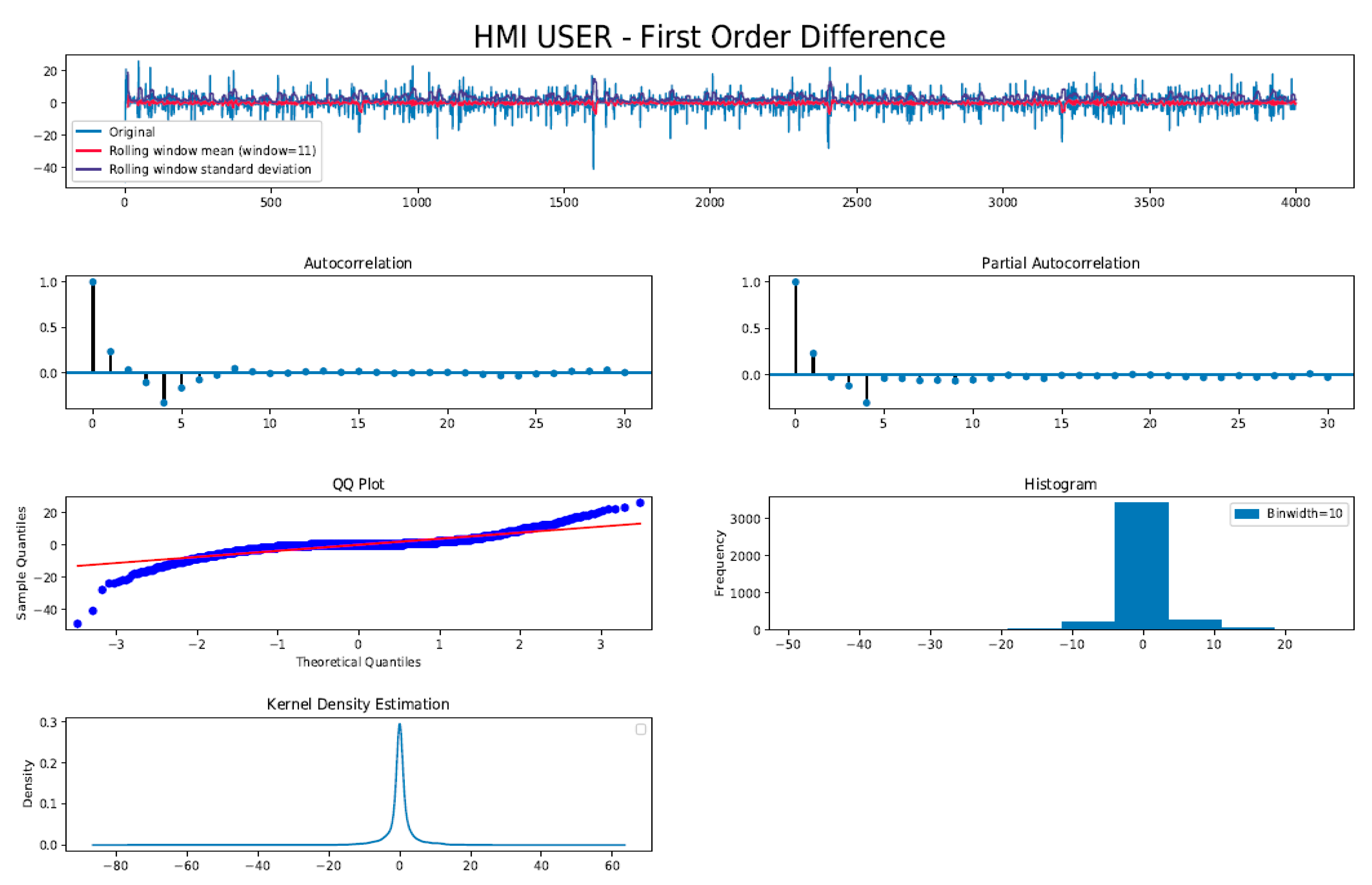
The second set of plots in Figure 8 are similar to Figure 7, but are generated by taking the log of the difference of the original TS data with its one-step lagged version. This is done to remove the seasonal trend component as apparent in original TS data set (Figure 5b). The first order differenced TS had a mean and standard deviation that did not vary with time, indicating the resulting TS data was closer to being stationary. This is further validated by looking at the histogram, Q–Q, and kernel density plots, which show a strong comparison to the ideal Gaussian (bell shape) distribution. Both ACF and PACF decay rapidly and show a hard cut-off after lag = 4. This aids in determining respective lag parameter (p and q) values for AR (p = 4) and MA (q = 4) processes from ACF and PCAF plots, respectively.
Therefore, from the above analysis, a first order difference is sufficient to make the HMI_USER data set generated from the test HMI in auto-pilot mode (Figure 5b) stationary and qualified to be modelled by ARIMA(p, d, q), where (p, d, q) have been estimated as per plots in Figure 8 (e.g., (p, d, q) = (4, 1, 4)). These parameter values were also confirmed programmatically using the exhaustive grid search optimization.
5.2. Persistence Score
The persistence forecast model with single step ahead (t + 1) and 50 step ahead (t + 50) with respect to original (t) data series is shown in Figure 9. For example, RMSEp1 = 3.75 score can be used as an upper bound of forecast error for any forecast any 1-step ahead (t + 1) model that is to be selected. Similarly, RMSEp for other persistence (p) lags (t + 2; t + 10; t + 20; t + 50) can also be generated in Figure 9 and RMSEp values shown in Table 1.
5.3. In-Sample (InS) Forecast
In-Sample (InS) forecast was done using a time-series prediction model (e.g., ARIMA or Seasonal ARIMA) to generate predictions for the time range that it had already seen during its training or fitting phase.
5.3.1. Static 1-Step Ahead
The basic InS 1-step ahead forecast was done using a static ARIMA model (Figure 10), where the model was not re-trained prior to predicting next step prediction. Root-mean-square (RMSE) error (or square root of variance) was used to compare prediction error and was calculated with respect to the actual observed values. Simulation showed an RMSE = 3.5 for InS 1-step ahead forecast using Static model (Figure 10) tracked the actual observed values closely. As expected, this model showed a slight performance improvement over the above reported persistence model for 1-lag i.e., <RMSEp=1 = 3.75.
5.3.2. Static n-Step Ahead
In this test, the static ARIMA model was used to make InS n-step ahead predictions for every observed sample in the training set (Figure 10). Evaluating any n-step ahead forecast requires using metrics calculated using a rolling (sliding) window metrics: e.g., average sample and RMSE. Since, an n-size rolling window when advanced one-time step ahead still takes into account or combines previous (n-1) duplicate (intermediate) predicted samples that were generated from each n-step ahead prediction run. Performance of the static n-step ahead model was evaluated by directly comparing the mean of the rolling window RMSE trend to the corresponding p-lag persistence RMSE value. Table 2 shows a consistent (RMSE = 3.4) forecast error value that is independent of n-step InS ahead forecast using the static ARIMA model.
The rationale for this performance was owing to the use of InS lagged values from the training set to generate next n-step ahead predictions; this prevents the forecast error to accumulate, i.e., be independent of n-steps. In addition, the performance was quite similar to that obtained as above for InS 1-step ahead static ARIMA forecast. Figure 11 shows an example of InS 50-step ahead static ARIMA forecast. The output predicted TS data closely tracked the InS training set. The confidence error bound, too, shows consistent variance over a full range of forecast. The rolling window average trend shows the predicted samples match temporal and scale variations with respect to the original test set. Rolling window RMSE trend (bottom-left of Figure 11) shows sharp spikes proportionate to the corresponding size of each HMI state transitions. This is an artefact of using rolling window computation which combines errors of previous duplicate samples.
5.3.3. Static Dynamic n-Step Ahead
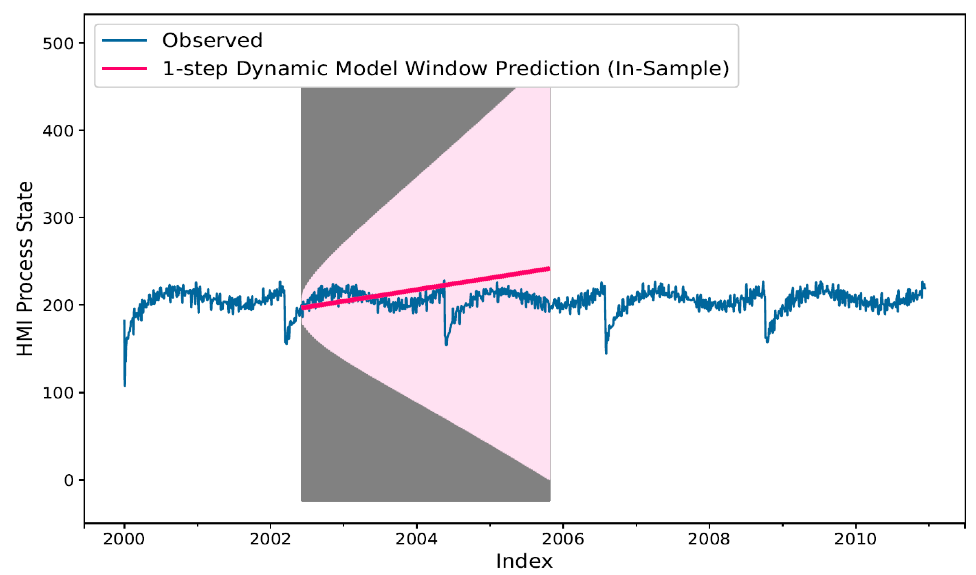
Using the static ARIMA model with dynamic mode of prediction recursively uses previously predicted samples instead of the lagged actual training set values to make next-step InS predictions. As seen in Figure 12, the prediction shows a deviation trend compared to the actual training set, even though only a 1-step ahead prediction was being used repeatedly stepwise over the full training set. The rationale for this performance was due to each (t − 1) predicted input values being fed to the static model containing prediction errors from when these were generated. The error tends to accumulate and amplify in each next time step predicted sample. As shown by, the prediction confidence interval (lighter shade of pink background area) that grows linearly over the entire range of training set using 1-step ahead forecast. This suggests, naive dynamic forecast is not feasible for doing longer range predictions. Simulation result for 1-step ahead dynamic forecast results in RMSE = 21.72 over the full range of training set.
5.3.4. Static Dynamic with Exogenous Input
Multivariate time-series auto-regressive (ARIMA) prediction models can also be trained with exogenous (external) time-varying predictor variables. However, exogenous predictor variables must satisfy unidirectional causality, i.e., only the exogenous variables (Xi) should affect a change in Y (variable to be predicted), and Y should not affect any change in Xi. This condition is usually tested by the Granger causality [29] test, which tests a statistical hypothesis for determining whether one time-series is useful in forecasting another. In this study, causality is ensured as per the experiment setup (Section 4.3). The soft HMI (Figure 5b) in auto-pilot mode generates PROCESS TS data independently of the HMI_USER TS data. Thus, only HMI_USER data or simulated user response is affected by current HMI PROCESS state value.
In this test, a static ARIMA model was fitted once on the training set consisting of both HMI_USER and its exogenous (exog.) predictor, PROCESS (example shown in Figure 13). Then, it was evaluated by generating in-sample 1-step ahead predictions using both the lagged values from actual training set (containing both HMI_USER and PROCESS (exog.) variable) and using past predicted values (dynamic mode). Figure 14 compares the predicted 1-step ahead series using static model in standard and dynamic modes. The static model in standard mode seems to show a close tracking with the training set with resulting RMSE = 4.46 as the forecast error. The static model under dynamic mode attempts to follow the training set; however, the predicted series was significantly scale attenuated resulting in RMSE = 6.73 as the forecast error. Using the exogenous predictor showed significant improvement in the dynamic mode forecast when compared to previous 1-step ahead dynamic mode forecast that is without using an exogenous predictor, as seen in Figure 12 (Section 5.3.3).
5.4. Out-of-Sample (OuS) Forecast
Out-of-Sample forecast was done using a time-series prediction model (e.g., ARIMA or SARIMA) to generate predictions for the time samples that the model had not seen during its initial training or fitting phase. That is using new data to forecast beyond the initial training sample set.
5.4.1. Adaptive 1-Step Ahead
As an extension to using a static ARIMA model, where the model was not re-fitted, the adaptive model was refitted prior to generating next-step forecast. Re-fitting was done on the new data set that had been seeded with the recent actual observed value(s). Due to the computational overhead (owing to re-fitting) the adaptive model was feasibly used for doing OuS predictions. The adaptive 1-step ahead forecast was evaluated for generating few numbers of out-of-sample durations: 10, 50, and 200. In Figure 15, only results of 200 sample duration forecasts are shown and the RMSE values for various sample run durations evaluated are listed in Table 3.
The forecast samples show a close tracking with respect to the evaluation test data set. Owing to refitting the model, it adapts to the new samples appropriately and the rolling window RMSE trend shows spikes due to sudden value transitions in the evaluation test set. Since all tests runs were done using a 1-step ahead forecast, the resulting RMSE values (Table 3) were only compared to required 1-lag persistence RMSE value (<RMSEp1 = 3.75). A lower RMSE value suggests acceptable performance of the adaptive model for doing out-of-sample 1-step ahead predictions.
5.4.2. Adaptive n-Step Ahead
The next evaluation was done using an adaptive model for n-step ahead predictions for various sample run durations as listed in Table 4 and shown in Figure 16. Similar to 1-step ahead, the adaptive model was re-fitted with current (t) observed sample being appended to original training data set added. In adaptive prediction (Section 5.4), n-step ahead predicted samples were generated with each new out-of-sample from the test set. In addition, as stated previously, all duplicate (having same time indexes) predicted samples were averaged using the n-size rolling window. In the OuS adaptive model, the RMSE results show a desirable scaling in performance with respect to n-step ahead parameters. For example, the (n = 10) 10-step ahead RMSE = 4.97 compared to the (n = 50) 50-step ahead RMSE = 5.2 for 500 sample runs was only a 4% increase in prediction error. In addition, each n-step adaptive OuS resulting RMSE value was approximately less compared to the equivalent lag persistence RMSEp scores as listed in Table 1, therefore indicating this to be an acceptable prediction model. Additionally, the RMSE value of n-step ahead prediction using an adaptive model was not conclusively related to the number of sample runs (Table 4), as it would have to depend on the nature of the training set data set being predicted.
In general, a longer n-step adaptive forecast (Figure 16 vs. Figure 15) yielded higher RMSE performance broader confidence bounds (shown as a light blue background in top-right plots). This is owing to the issue of scale attenuation in sample values generated in longer n-step ahead forecasts, which is apparent from similar amplitude range of the test set trend with its corresponding forecast sample rolling window average trend in 1-step (Figure 15) than in 50-step (Figure 16) ahead forecast.
5.4.3. Adaptive Dynamic n-Step Ahead
Out-of-sample adaptive model using the dynamic forecast method was re-fitted on the initial training set, to which previous (n-1) predicted samples were also appended. The RMSE values of this test are listed in Table 5. The prediction performance was quite similar to what was observed for the standalone adaptive (Table 4) forecast model, with dynamic method generally yielding an overall higher RMSE, since the error tend to accumulate and amplify (as is the general case with dynamic predictions) over time. The dependence of performance error (RMSE) on the n-step ahead parameter did not show any conclusive correlation to required prediction sample run length, e.g., for n-step = 4, 20, 50; all showed an approximate RMSE = 5.4 for 500 sample run lengths.
5.4.4. Adaptive n-Step with Exogenous Input
Out-of-sample prediction performance with exogenous predictor variable (PROCESS) was evaluated with an adaptive model. Forecast error RMSE values of each n-step ahead forecast (shown in Table 6) were smaller compared to RMSE for corresponding persistence lag values (Table 1). However, the performance of the standalone adaptive model for OuS n-step forecast without using the exogenous input (Table 4) was overall better, than when exogenous input was used.
5.4.5. Adaptive Dynamic n-Step with Exogenous Input
5.5. Discussion
The following observations can be made based on the above results.
5.5.1. Static ARIMA Model
- In-Sample (InS) Forecast: InS 1-Step ahead prediction using a static model (where model fitted) once showed comparable performance to 1-lag persistence model (Table 1), therefore its acceptable to use this technique when available TS data is expected to be very similar to the initial training set that was used to fit the ARIMA static model.
- InS Uniform Performance: Static models showed a uniform prediction performance for InS with respect to length of forecast sample run. This is owing to the fact that since the actual InS sample was used to make next-step prediction, the ARIMA model parameters were sufficiently optimal to make accurate 1-step ahead predictions for any length of required sequence run (as long as input samples are coming from a previous training set).
- Out-of-Sample (OuS) n-Step Ahead Performance Is Poor: Unlike previous observation, the Static model expectedly did not perform well, especially when asked to do OuS n-step ahead predictions.
- Dynamic Mode for InS and OuS Performance Is Poor: Static model in dynamic mode where prediction recursively used previously predicted samples instead of the lagged actual training set values to make next-step InS predictions. This mode when used with the Static model for InS prediction yielded poor performance compared to p-lag persistence RMSE scores. OuS performance using static model was not evaluated with this study; however, based on preliminary results there was similar poor performance of ARIMA for any OuS n-Step ahead predictions using dynamic mode. This is owing to model not being re-fitted (as in the case of the adaptive model) which caused forecast errors to accumulate and amplify as subsequent past forecast samples are used to make next step predictions.
- Static with Exogenous (Exog.) Input Shows Improvement: Performance of static models with exogenous input did show some performance improvement for InS prediction for both standard mode (where actual lagged values are used) and in dynamic mode when compared to simply using standalone static model in dynamic mode.
5.5.2. Adaptive ARIMA Model
- Out-of-Sample (OuS) n-Step Ahead Performance is Acceptable: The adaptive model for n-step ahead OuS prediction performed comparably to corresponding p-lag persistence RMSE scores (Table 1). This was expected since the model was re-fitted each time with new OuS samples being appended to the original training set history.
- Dynamic Mode Performance is Stable: Prediction performance using the adaptive model in dynamic mode showed consistent performance compared to just the standalone adaptive model for OuS n-step ahead predictions.
- Exogenous Inputs yield Consistent Performance: Performance of adaptive model in dynamic mode with exogenous input did not show much improvement in overall performance. However, it yielded consistent prediction error (RMSE) with respect to n-step ahead forecast even though the error was generally higher compared to when no exogenous input was used in adaptive model with dynamic mode.
5.6. Model Limitations
Limitations of the static and adaptive ARIMA models based on above results are discussed below.
5.6.1. Static ARIMA Model
The static ARIMA model was fitted only once on a given training set. Its InS forecast capability shows comparable performance to 1-lag persistence score (Table 1) and generally shows uniform performance independent of forecast sample run length. The latter was an outcome of the ARIMA model being sufficiently optimal to make accurate 1-step ahead predictions, provided the input samples were expected to be similar (having lower variance) compared to initial training InS distribution. However, the major limitations of static ARIMA models are summarized below in Table 8:
5.6.2. Adaptive ARIMA Model
Adaptive ARIMA models are generally utilized when out-of-sample prediction is required using linear regression. These models are adaptive since they are re-fitted frequently with new expected data being appended to the original training set of InS forecast. However, the major limitations of adaptive ARIMA models are summarized below in Table 9:
5.6.3. General Limitations of ARIMA Models
In general, ARIMA models are regression-based models that require manual analysis of the time series to be modeled. Namely, it is essential to do pre-processing of target time-series, to be modeled, in order to convert into stationary time series.
Moreover, the auto regressive (AR) and moving average (MA) and difference model parameters must be identified manually by various analysis techniques such as histograms, density plots, auto-correlation function (ACF), and partial auto-correlation function (PACF), Q–Q plot, and ADF scores (see Section 5.1). Despite the simplicity of the ARIMA model, its deterministic performance and optimal model parameters being grid searched programmatically, these are not ideal for modelling time-series that have non-linear residual forecast errors. Instead, recurrent neural networks are better suited for modelling multivariate time-series having non-linear residuals.
6. Conclusions and Future Work
The intent of this research was to evaluate Auto-Regressive Integrated Moving Average (ARIMA) models with exogenous regressors to predict HMI state time-series patterns. The novel concept presented in this paper further extends our previous work with ARIMA models [30] to evaluate a non-intrusive operator situational awareness monitoring solution. It is based on the premise that HMI state may be represented as a weakly stationary time-series which can be modelled and predicted using linear regression forecast models. This is towards the overall goal of achieving real-time monitoring of operator situational awareness while using human–machine interfaces.
The results indicate ARIMA to be feasible in doing both in-sample and out-of-sample mode of prediction for shorter (n <= 20) n-step ahead temporal windows. Adaptive models help to reduce out-of-sample prediction errors for longer-range (n > 20) n-step ahead forecasts. However, the capability to do n-step ahead forecast in general becomes challenging due to higher prediction errors with ARIMA models. Using exogenous regressors only showed marginal accuracy improvement for in-sample prediction and poor performance for out-of-sample forecast on the synthetic test data set within the scope of this study.
The future work entails utilizing long short-term memory (LSTM) recurrent neural networks to improve accuracy of prediction by offsetting the limitation of the ARIMA model in doing out-of-sample mode of prediction for longer (n > 50) n-step ahead prediction windows, which also make use of multi-variable exogenous (causally independent) variables. The LSTM time-series models have shown to perform well where long sample window temporal patterns need to be learned and predicted, which a purely ARIMA model does not model too well. Moreover, we will collect data from a control room HMI panel training simulator used in a nuclear power plant to train and evaluate the HMI state prediction models for real-world industrial application.
Author Contributions
Writing—Original Draft Preparation, H.V.P.S.; Supervision and Writing—Review & Editing, Q.H.M.
Funding
This research received no external funding.
Conflicts of Interest
The authors declare no conflicts of interest.
References
- International Atomic Energy Agency (IAEA). International Nuclear Event Scale (INES). Available online: http://www-ns.iaea.org/tech-areas/emergency/ines.asp (accessed on 2 August 2018).
- IAEA. INSAG-7, The Chernobyl Accident, Updating of INSAG-1. Available online: http://www-pub.iaea.org (accessed on 2 August 2018).
- Nuclear Energy Institute. Lessons from the 1979 Accident at Three Mile Island. 2014. Available online: http://www.nei.org (accessed on 2 August 2018).
- Atomic Energy of Canada Limited, Chalk River Laboratories. The Chalk River Accident in 1952—The Canadian Nuclear FAQ. Available online: http://www.nuclearfaq.ca (accessed on 2 August 2018).
- Manzey, D.; Reichenbach, J.; Onnasch, L. Human performance consequences of automated decision aids: The impact of degree of automation and system experience. J. Cogn. Eng. Decis. Mak. 2012, 6, 57–87. [Google Scholar] [CrossRef]
- Singh, H.V.; Mahmoud, Q.H. Eye-on-HMI: A framework for monitoring human machine interfaces in control rooms. In Proceedings of the 2017 IEEE 30th Canadian Conference on Electrical and Computer Engineering (CCECE), Windsor, ON, Canada, 30 April–3 May 2017; pp. 1–5. [Google Scholar]
- Singh, H.V.; Mahmoud, Q.H. ViDAQ: A framework for monitoring human machine interfaces. In Proceedings of the 2017 IEEE 20th International Symposium on Real-Time Distributed Computing (ISORC), Toronto, ON, Canada, 16–18 May 2017; pp. 141–149. [Google Scholar]
- Swain, A.D.; Guttmann, H.E. Handbook of Human-Reliability Analysis with Emphasis on Nuclear Power Plant Applications; Final Report (No. NUREG/CR-1278; SAND-80-0200); Sandia National Labs.: Albuquerque, NM, USA, 1983.
- Ye, H.; Zheng, W. A human reliability analysis method based on cognitive process model for risk assessment. In Proceedings of the 2016 IEEE International Conference on Intelligent Rail Transportation (ICIRT), Birmingham, UK, 23–25 August 2016; pp. 418–424. [Google Scholar]
- Yao, W.; Zupei, S. Cream—A second generation human reliability analysis method. Ind. Eng. Manag. 2005, 10, 17–21. [Google Scholar]
- Mu, L.; Xiao, B.; Xue, W.; Yuan, Z. The prediction of human error probability based on bayesian networks in the process of task. In Proceedings of the 2015 IEEE International Conference on Industrial Engineering and Engineering Management (IEEM), Singapore, 6–9 December 2015; pp. 145–149. [Google Scholar]
- Mackieh, A.; Cilingir, C. Effects of performance shaping factors on human error. Int. J. Ind. Ergon. 1998, 22, 285–292. [Google Scholar] [CrossRef]
- Blackman, H.S.; Gertman, D.I.; Boring, R.L. Human error quantification using performance shaping factors in the spar-h method. In Proceedings of the Human Factors and Ergonomics Society Annual Meeting; SAGE Publications Sage CA: Los Angeles, CA, USA, 2008; Volume 52, pp. 1733–1737. [Google Scholar]
- Lee, H.-C.; Jang, T.-I.; Moon, K. Anticipating human errors from periodic big survey data in nuclear power plants. In Proceedings of the 2017 IEEE International Conference on Big Data (Big Data), Boston, MA, USA, 11–14 December 2017; pp. 4777–4778. [Google Scholar]
- Chang, Y.; Mosleh, A. Cognitive modeling and dynamic probabilistic simulation of operating crew response to complex system accidents: Part 1: Overview of the idac model. Reliab. Eng. Syst. Saf. 2007, 92, 997–1013. [Google Scholar] [CrossRef]
- Xie, G.; Gao, H.; Qian, L.; Huang, B.; Li, K.; Wang, J. Vehicle trajectory prediction by integrating physics-and maneuver-based approaches using interactive multiple models. IEEE Trans. Ind. Electron. 2018, 65, 5999–6008. [Google Scholar] [CrossRef]
- Li, D.; Gao, H. A hardware platform framework for an intelligent vehicle based on a driving brain. Engineering 2018, 4, 464–470. [Google Scholar] [CrossRef]
- Wardah, T.; Kamil, A.; Hamid, A.S.; Maisarah, W. Statistical verification of numerical weather prediction models for quantitative precipitation forecast. In Proceedings of the 2011 IEEE Colloquium on Humanities, Science and Engineering (CHUSER), Penang, Malaysia, 5–6 December 2011; pp. 88–92. [Google Scholar]
- Gao, T.; Chai, Y.; Liu, Y. Applying long short term memory neural networks for predicting stock closing price. In Proceedings of the 2017 8th IEEE International Conference on Software Engineering and Service Science (ICSESS), Beijing, China, 24–26 November 2017; pp. 575–578. [Google Scholar]
- He, C.; Xu, Q.; Liu, Y. A new model between stock valuation index and volatility of stock price. In Proceedings of the 2010 International Conference on Intelligent Computing and Cognitive Informatics (ICICCI), Kuala Lumpur, Malaysia, 22–23 June 2010; pp. 479–482. [Google Scholar]
- Gao, H.; Cheng, B.; Wang, J.; Li, K.; Zhao, J.; Li, D. Object classification using cnn-based fusion of vision and lidar in autonomous vehicle environment. IEEE Trans. Ind. Inform. 2018, 14, 4224–4231. [Google Scholar] [CrossRef]
- Box, G.E.; Jenkins, G.M.; Reinsel, G.C.; Ljung, G.M. Time Series Analysis: Forecasting and Control, 5th ed.; John Wiley & Sons: Hoboken, NJ, USA, 2015; ISBN 978-1-118-67502-1. [Google Scholar]
- Wijaya, Y.B.; Kom, S.; Napitupulu, T.A. Stock price prediction: Comparison of ARIMA and artificial neural network methods-an indonesia stock’s case. In Proceedings of the 2010 Second International Conference on Advances in Computing, Control and Telecommunication Technologies (ACT), Jakarta, Indonesia, 2–3 December 2010; pp. 176–179. [Google Scholar]
- Tan, Z.; Zhang, J.; Wang, J.; Xu, J. Day-ahead electricity price forecasting using wavelet transform combined with ARIMA and GARCH models. Appl. Energy 2010, 87, 3606–3610. [Google Scholar] [CrossRef]
- Bi, J.; Zhang, L.; Yuan, H.; Zhou, M. Hybrid task prediction based on wavelet decomposition and ARIMA model in cloud data center. In Proceedings of the 2018 IEEE 15th International Conference on Networking, Sensing and Control (ICNSC), Zhuhai, China, 27–29 March 2018; pp. 1–6. [Google Scholar]
- Janardhanan, D.; Barrett, E. CPU workload forecasting of machines in data centers using LSTM recurrent neural networks and ARIMA models. In Proceedings of the 2017 12th International Conference for Internet Technology and Secured Transactions (ICITST), Cambridge, UK, 11–14 December 2017; pp. 55–60. [Google Scholar]
- Rath, A.; Samantaray, S.; Bhoi, K.S.; Swain, P.C. Flow forecasting of hirakud reservoir with ARIMA model. In Proceedings of the 2017 International Conference on Energy, Communication, Data Analytics and Soft Computing (ICECDS), Chennai, India, 1–2 August 2017; pp. 2952–2960. [Google Scholar]
- Cheung, Y.; Lai, K. Lag order and critical values of the augmented dickey–fuller test. J. Bus. Econ. Stat. 1995, 13, 277–280. [Google Scholar]
- Yang, D.; Chen, H.; Song, Y.; Gong, Z. Granger causality for multivariate time series classification. In Proceedings of the 2017 IEEE International Conference on Big Knowledge (ICBK), Hefei, China, 9–10 August 2017; pp. 103–110. [Google Scholar]
- Singh, H.V.; Mahmoud, Q.H. Non-Intrusive Monitoring of Operator Situational Awareness Via Human-Machine Interface States. In 8th International Conference on Simulation Methods in Nuclear Science and Engineering; Canadian Nuclear Society (CNS-SNC): Toronto, ON, Canada, 2018. [Google Scholar]
Figure 1.
Architecture of: (A) conventional operator-based command–control–feedback process systems; (B) expert supervisory system (EYE)-on-human–machine interface (HMI) adds cross-validation to operator command–control–feedback process systems.
Figure 1.
Architecture of: (A) conventional operator-based command–control–feedback process systems; (B) expert supervisory system (EYE)-on-human–machine interface (HMI) adds cross-validation to operator command–control–feedback process systems.

Figure 2.
A typical physical HMI model. HMI state variables can be classified as representing process outputs and human inputs. Each state variable can either be digital or fixed-point real numbers.
Figure 2.
A typical physical HMI model. HMI state variables can be classified as representing process outputs and human inputs. Each state variable can either be digital or fixed-point real numbers.

Figure 3.
Example of time series (TS). (a) Gaussian white noise (strictly stationary) (μ = 0, σ2 = k (constant), γ[τ] = 0 for all τ). (b) Random walk (non-stationary)—non-constant mean and variance. (c) Weakly stationary (μ ≠ 0, σ2 = k (constant), γ(t, s) = γ[τ] = X auto-covariance between any two points (t, s) is constant for fixed τ = t − s distance (lag)) as there is no obvious trend and repeating seasonality effects.

Figure 4.
Several time-series generated using the same stationary process or a random variable (X). Weakly stationary requires the non-zero mean (μ) and variance σ2 to be constant for all times (slices) e.g., t or k. In addition, the covariance (γ[τ]) must only be a function of temporal distance between any two points in time.

Figure 5.
Test HMI application in manual and auto-pilot mode. Process values are generated using AR(p), MA(q), and Gaussian noise process with trend and seasonal components. (a) Manual mode: process values displayed via array of lamp indicators. User tracks indication patterns by manually setting 8 toggle switches in same pattern until alarm indication (red lamp) goes off. (b) Auto-pilot mode: user tracking response to process values is modeled using a proportional-integral (PI) controller with random proportional gain. HMI process and user response was captured as a time-series data example of a diagram.

Figure 6.
Sample time-series data set. PROCESS and HMI_USER series dataset samples were limited to 8-bit integers.
Figure 6.
Sample time-series data set. PROCESS and HMI_USER series dataset samples were limited to 8-bit integers.

Figure 7.
Diagnostic plots of original the HMI_USER series dataset. Moving average mean shows seasonal trend therefore TS is non-stationary. TS is not random walk, since rolling standard deviation (variance) does not vary with time. Auto-Correlation Function (ACF) decays slowly indicative of seasonal trend. Partial Auto-Correlation Function (PACF) indicates a moving average (MA) process of finite lag. Quantile (QQ), histogram, and kernel density plots indicate a Gaussian-like distribution with a long tail suggesting presence of a periodic trend component in TS.

Figure 8.
Diagnostic plots of log first order difference of the HMI_User series dataset. Moving average mean no longer shows seasonal trend, therefore TS is closer to being stationary. Moreover, both rolling mean and standard deviation (variance) does not vary with time. ACF decays rapidly and cut off hard, indicative of AR(p) process. PACF also shows rapid decay after lag = 4 indicating MA(q) process. Quantile (QQ), histogram, and kernel density plots indicate a more Gaussian-like distribution with negligible tail suggesting the trend component has been minimized significantly.

Figure 9.
Persistence (naive) forecast model plot for 50 lag. Root Mean Square Error (RMSE) of persistence model was used to ascertain the acceptable upper bound (worst case) of forecast error associated with the particular data set when using a forecast model.
Figure 9.
Persistence (naive) forecast model plot for 50 lag. Root Mean Square Error (RMSE) of persistence model was used to ascertain the acceptable upper bound (worst case) of forecast error associated with the particular data set when using a forecast model.

Figure 10.
In-sample (InS), Static 1-Step ahead forecast TS. TS (blue) shows observed actual values of the training set. TS (red) shows the InS forecasted values which closely track the training set. Light blue background shows confidence interval bounds for the forecast TS.
Figure 10.
In-sample (InS), Static 1-Step ahead forecast TS. TS (blue) shows observed actual values of the training set. TS (red) shows the InS forecasted values which closely track the training set. Light blue background shows confidence interval bounds for the forecast TS.

Figure 11.
In-sample (InS) static 50-Step ahead forecast. Top-left plot shows 50-step ahead predicted samples overlaid on the actual InS test set. Top-right plot shows the forecast TS with per sample confidence interval as background colour. Bottom (right and left) plots show rolling window metrics: average and RMSE, respectively, for the 50-Step ahead forecast.

Figure 12.
InS 1-Step ahead static model in dynamic mode forecast (red bold line). The confidence interval (prediction error) associated with forecast values may be seen in background as a lighter shade of pink area on the plot, which deviates with a constant up trend indicative of accumulation of forecast error per previously predicted values.

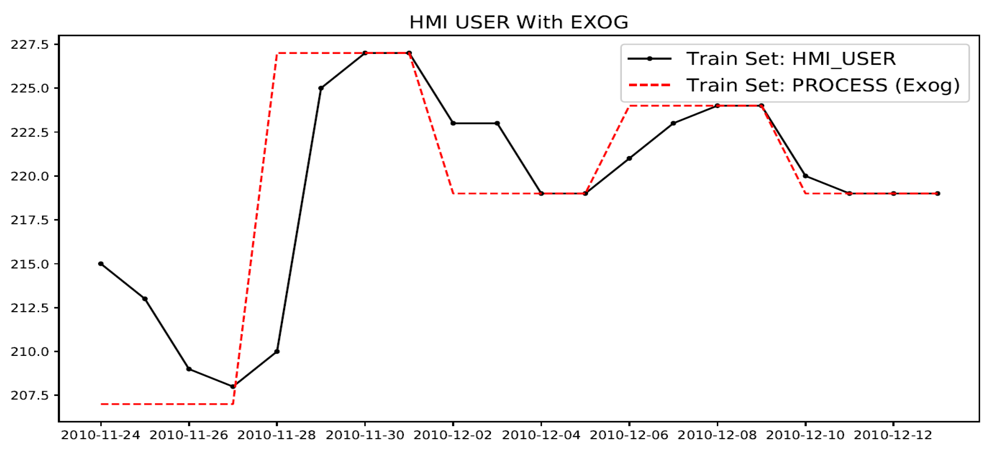
Figure 13.
Example showing HMI_USER (variable to be modeled) and its exogenous (Exog.) predictor variable: PROCESS state.
Figure 13.
Example showing HMI_USER (variable to be modeled) and its exogenous (Exog.) predictor variable: PROCESS state.

Figure 14.
In sample 1-Step ahead static with normal and dynamic mode forecast with exogenous predictor (PROCESS) variable. The confidence interval associated with the static dynamic model trend (bold green line) may be seen in background as a light blue shade on the plot area.
Figure 14.
In sample 1-Step ahead static with normal and dynamic mode forecast with exogenous predictor (PROCESS) variable. The confidence interval associated with the static dynamic model trend (bold green line) may be seen in background as a light blue shade on the plot area.

Figure 15.
Out-of-Sample adaptive 1-Step ahead prediction for 200 sample run lengths shows close tracking.
Figure 15.
Out-of-Sample adaptive 1-Step ahead prediction for 200 sample run lengths shows close tracking.

Figure 16.
Out-of-sample adaptive 50-Step ahead prediction for 500 sample run lengths scale attenuated.
Figure 16.
Out-of-sample adaptive 50-Step ahead prediction for 500 sample run lengths scale attenuated.

Figure 17.
Out-of-sample adaptive 50-Step ahead for 500 sample runs with exogenous input.


Table 1.
Persistence n-Lag RMSEp.
| n-Lag | RMSEp |
|---|---|
| 1 | 3.75 |
| 2 | 5.96 |
| 10 | 9.78 |
| 20 | 11.37 |
Table 2.
In-sample static n-Step RMSE.
| n-Step | RMSE |
|---|---|
| 1 | 3.41 |
| 2 | 3.39 |
| 10 | 3.42 |
| 20 | 3.40 |
Table 3.
Out-of-sample adaptive 1-Step RMSE.
| Sample Run | RMSE |
|---|---|
| 10 | 1.82 |
| 20 | 3.79 |
| 50 | 2.93 |
| 200 | 3.18 |
Table 4.
OuS adaptive n-Step RMSE.
| n-Step | Sample Run | RMSE |
|---|---|---|
| 1 | 20 | 3.79 |
| 2 | 20 | 4.24 |
| 2 | 200 | 3.63 |
| 4 | 20 | 4.81 |
| 4 | 500 | 5.19 |
| 10 | 10 | 2.20 |
| 10 | 200 | 4.47 |
| 10 | 500 | 4.97 |
| 20 | 500 | 5.20 |
| 50 | 500 | 5.20 |
Table 5.
OuS adaptive dynamic n-Step RMSE.
| n-Step | Sample Run | RMSE |
|---|---|---|
| 4 | 10 | 3.01 |
| 10 | 200 | 5.09 |
| 1 | 500 | 5.02 |
| 4 | 500 | 5.45 |
| 20 | 500 | 5.42 |
| 50 | 500 | 5.67 |
Table 6.
OuS adaptive Exog. n-Step RMSE.
| n-Step | Sample Run | RMSE |
|---|---|---|
| 1 | 200 | 3.12 |
| 2 | 200 | 3.70 |
| 4 | 200 | 4.56 |
| 10 | 200 | 4.78 |
| 20 | 200 | 5.40 |
| 50 | 200 | 9.42 |
Table 7.
OuS adaptive dynamic Exog. n-Step RMSE.
| n-Step | Sample Run | RMSE |
|---|---|---|
| 1 | 200 | 5.40 |
| 2 | 200 | 5.96 |
| 4 | 200 | 6.48 |
| 10 | 200 | 5.92 |
| 20 | 200 | 6.34 |
| 50 | 200 | 9.62 |
Table 8.
Static ARIMA model limitations.
| Limitation | Performance | Rationale |
|---|---|---|
| Out-of-Sample (OuS) n-Step Ahead Performance | Poor | ARIMA model parameters cannot be sufficiently optimized for doing longer run OuS predictions. |
| Dynamic Mode for InS and OuS Performance | Poor | Yields higher error than same p-lag persistence RMSEp value. This is owing to model not being re-fitted which causes forecast errors to accumulate and amplify. |
Table 9.
Adaptive ARIMA model limitations.
| Limitation | Performance | Rationale |
|---|---|---|
| Multi-variate (Exogenous) time-series prediction support | Poor | Adaptive model with dynamic mode yields consistent RMSE values for n-step ahead predictions; however, it yields higher RMSE values for longer n-step ahead prediction. |
© 2019 by the authors. Licensee MDPI, Basel, Switzerland. This article is an open access article distributed under the terms and conditions of the Creative Commons Attribution (CC BY) license (http://creativecommons.org/licenses/by/4.0/).
Share and Cite
MDPI and ACS Style
Singh, H.V.P.; Mahmoud, Q.H. Evaluation of ARIMA Models for Human–Machine Interface State Sequence Prediction. Mach. Learn. Knowl. Extr. 2019, 1, 287-311. https://0-doi-org.brum.beds.ac.uk/10.3390/make1010018
AMA Style
Singh HVP, Mahmoud QH. Evaluation of ARIMA Models for Human–Machine Interface State Sequence Prediction. Machine Learning and Knowledge Extraction. 2019; 1(1):287-311. https://0-doi-org.brum.beds.ac.uk/10.3390/make1010018
Chicago/Turabian StyleSingh, Harsh V. P., and Qusay H. Mahmoud. 2019. "Evaluation of ARIMA Models for Human–Machine Interface State Sequence Prediction" Machine Learning and Knowledge Extraction 1, no. 1: 287-311. https://0-doi-org.brum.beds.ac.uk/10.3390/make1010018