Artificial Intelligence to Enhance Aerodynamic Shape Optimisation of the Aegis UAV


School of Aerospace, Transport and Manufacturing, Cranfield University, Bedford MK43 0AL, UK
*
Author to whom correspondence should be addressed.
Mach. Learn. Knowl. Extr. 2019, 1(2), 552-574; https://0-doi-org.brum.beds.ac.uk/10.3390/make1020033
Submission received: 5 March 2019
/
Revised: 22 March 2019
/
Accepted: 30 March 2019
/
Published: 4 April 2019
(This article belongs to the Section Network)
Abstract
:This article presents an optimisation framework that uses stochastic multi-objective optimisation, combined with an Artificial Neural Network (ANN), and describes its application to the aerodynamic design of aircraft shapes. The framework uses the Multi-Objective Particle Swarm Optimisation (MOPSO) algorithm and the obtained results confirm that the proposed technique provides highly optimal solutions in less computational time than other approaches to the same design problem. The main idea was to focus computational effort on worthwhile design solutions rather than exploring and evaluating all possible solutions in the design space. It is shown that the number of valid solutions obtained using ANN-MOPSO compared to MOPSO for 3000 evaluations grew from 529 to 1006 (90% improvement) with a penalty of only 8.3% (11 min) in computational time. It is demonstrated that including an ANN, the ANN-MOPSO with 3000 evaluations produced a larger number of valid solutions than the MOPSO with 5500 evaluations, and in 33% less computational time (64 min). This is taken as confirmation of the potential power of ANNs when applied to this type of design problem.
1. Introduction
The aircraft industry gives considerable attention to computational optimisation tools in order to enhance the efficiency of the design process and product quality and performance. In reality, most real-world applications contain many complicating factors and constraints that affect system behaviour. Consequently, finding optimal solutions, or even only those viable for a given design problem, in an economical computational time is a difficult task, even with the availability of superfast computers. Thus, it is important to optimise the use of available computational resources.
Researchers in engineering design aim to address optimisation problems by balancing the efficiency of the design process against the fidelity of the numerical model. To resolve this conflict, problem approximation and function approximation techniques have been used [1]. Problem approximation attempts to substitute the original problem with a less demanding computationally solvable problem. However, Piperni et al. [2] and Zhang et al. [3] have argued that the level of fidelity required of the models is mostly determined at the development stage, which the design process aims to enhance. On the other hand, the use of function approximation techniques through the use of surrogate models [4] may degrade the accuracy of the results [5].
However, all real-world design problems require a high degree of accuracy, which is obtained only by evaluation of its real objective function, and this can be a lengthy process [5]. This problem can be severe when the number of unfeasible trial solutions are substantially more than the feasible, which is often the case in aerodynamic shape design optimisation problems [6,7]. It is not sensible to spend a long time evaluating non-worthwhile solutions thus engineering design problems will invariably require a combined process that accelerates optimisation while retaining all the useful information of the design space. This process should produce higher optimal solutions in less computational time, but accurate solutions cannot be achieved without using the real objective function [5].
This paper pays particular attention to the development of an optimisation framework in an industrial setting, that can be used to accelerate the optimisation search while retaining the useful information contained in the design space regarding the aerodynamic shape design problem. It reports an investigation into the application of advanced optimisation techniques to shorten the path to optimal solutions by adding Machine Learning (ML) [8] to the optimisation process. The main idea is to focus all the computational efforts on the worthwhile solutions, rather than exploring and evaluating all trial solutions in the design space [5].
ML is a field of computer science that gives the computer the ability to “learn” without being explicitly programmed. The term machine learning was first introduced in 1959 by Arthur Samuel, one of the pioneers in the field of computer gaming and artificial intelligence [8].
Increasingly, ML is being widely used for classification [9], numerical prediction [10], and pattern recognition [11]. With ML the computer can “learn” the complex and multifaceted relationships between dependent and independent variables via a “black box” (or neural net), which processes the data. Such applications have been used extensively in, for example; biology [12], engineering [13,14,15], environmental analysis [16], information technology [17] and medicine [18]. Such applications reveal the extent to which ML has been used to boost research and development.
ML is attractive to engineers because of its remarkable characteristic of learning to process imprecise and uncertain information [9,10,11]. Furthermore, it is able to achieve excellent generalized solutions through the use of powerful training algorithms, which produce solutions that are reliable inside and outside the region of design space used for the training data [19], and perform massive parallel computations, which has a significant impact on the computational time [20]. These factors have attracted researchers to the application of Artificial Neural Networks (ANNs) with advanced optimisation algorithms for various aircraft design problem enhancements [4,21,22,23,24]. Actually, an ANN is used mostly to model the objective functions for the design problem, where the computing of the objective function is time-consuming and computationally expensive [25,26]. However, as stated above, it is important to remember that using surrogate models instead of the real objective functions for complex industrial problems may degrade the accuracy of the results [5].
Regardless of the ML used, obtaining high optimality requires a deep understanding of the numerical optimisation technique, training procedure, specification of the machine in use, and full knowledge of the design problem. For that reason, researchers have investigated various traditional optimisation algorithms to obtain the best combinations of the process parameters. Although these traditional optimisation algorithms performed well in many particular cases, they did have some restrictions related to their search procedures [27]. The solutions obtained by an ANN algorithm can be far from the optimal solutions that are expected by a Decision Maker (DM) if it becomes trapped in local minimum [28]. To overcome such a problem bio-inspired algorithms which are based on natural behaviour, such as Particle Swarm Optimisation (PSO) algorithms [29] and Evolutionary Algorithms (EA) [30], have been developed [31].
Keeping in view the success of EAs [32], ANNs had been used in many projects to construct a surrogate model to reduce the overall computational cost and to obtain greater optimality in the solutions [14,25,32,33,34,35]. The PSO, for example, has a simple mechanism and is computationally inexpensive in terms of memory requirements relative to other population techniques [36,37], and has been implemented by many researchers in various algorithms with an ANN to model the objective function, also the PSO has been used to help with the training of ANNs [38,39,40,41]. Since the PSO is based on a simple concept and is computationally inexpensive, many researchers have extended the algorithm to handle multi-objective optimisation problems [7,37,42]. In [5], the authors extensively reviewed PSO algorithms used to evolve ANNs.
A review of published work found only one publication where the neural network was used to guide the optimisation algorithm in order to reduce the computational time (this concerned an airfoil optimisation problem) by deciding whether the trial solution was worthy of full evaluation or not, rather than using the neural network to model the objective function [5]. In view of the limited research in this area, the present paper reports an investigation that demonstrates the efficiency that can be obtained by using an ANN to guide the optimisation search by deciding whether a trial solution was worthy of full evaluation or not, as applied to aerodynamic shape design optimisation for the Aegis Unmanned Aerial Vehicle (UAV). This was a design problem in which the wing and tail design variables were used simultaneously to obtain a set of optimal solutions for the Aegis UAV under continuous training of the ANN. In [43,44], the authors reported developing a strategy that used non-interactive and interactive techniques, respectively, to formulate the design problem and improve the optimisation speed. To deliver a sufficient level of fidelity to the DM at very fast computational times, the low fidelity flow solver Athena Vortex Lattice (AVL) was used to capture the physics of the problem [45,46,47,48]. Improving the ability of the developed method to accelerate the search while retaining all the useful information in the design space was the main area of work. However, we have shown in [44] that we could miss some important information contained in the design space, since the interactive method starts to focus on certain areas early in the search. Moreover, the DM does not always succeed in guiding the search to the region of interest because of the stochastic characteristics of the algorithm. To overcome these problems, an ANN is used to increase the performance of the optimisation.
The results obtained showed the success of the ANN in recognising non-valid solutions. The solver avoided wasting computational efforts on non-worthwhile solutions and so the optimisation process provided solutions that are more valid in almost the same computational time. In addition, the research has made a significant contribution by comparing solving the problem by interactive and non-interactive optimisation approaches [44]. It should be noted that the results obtained here are compared to results previously published by the authors [44].
The remainder of this paper is structured as follows. In Section 2, the methodology framework is explained. In Section 3, various training processes and other issues regarding the ANN are described. Problem architecture, related work and design of experiments are described in Section 4. Section 5 describes the optimisation results, data visualisation, and analysis for the optimum compromise solutions. Conclusions are given in Section 6.
2. Materials and Methods
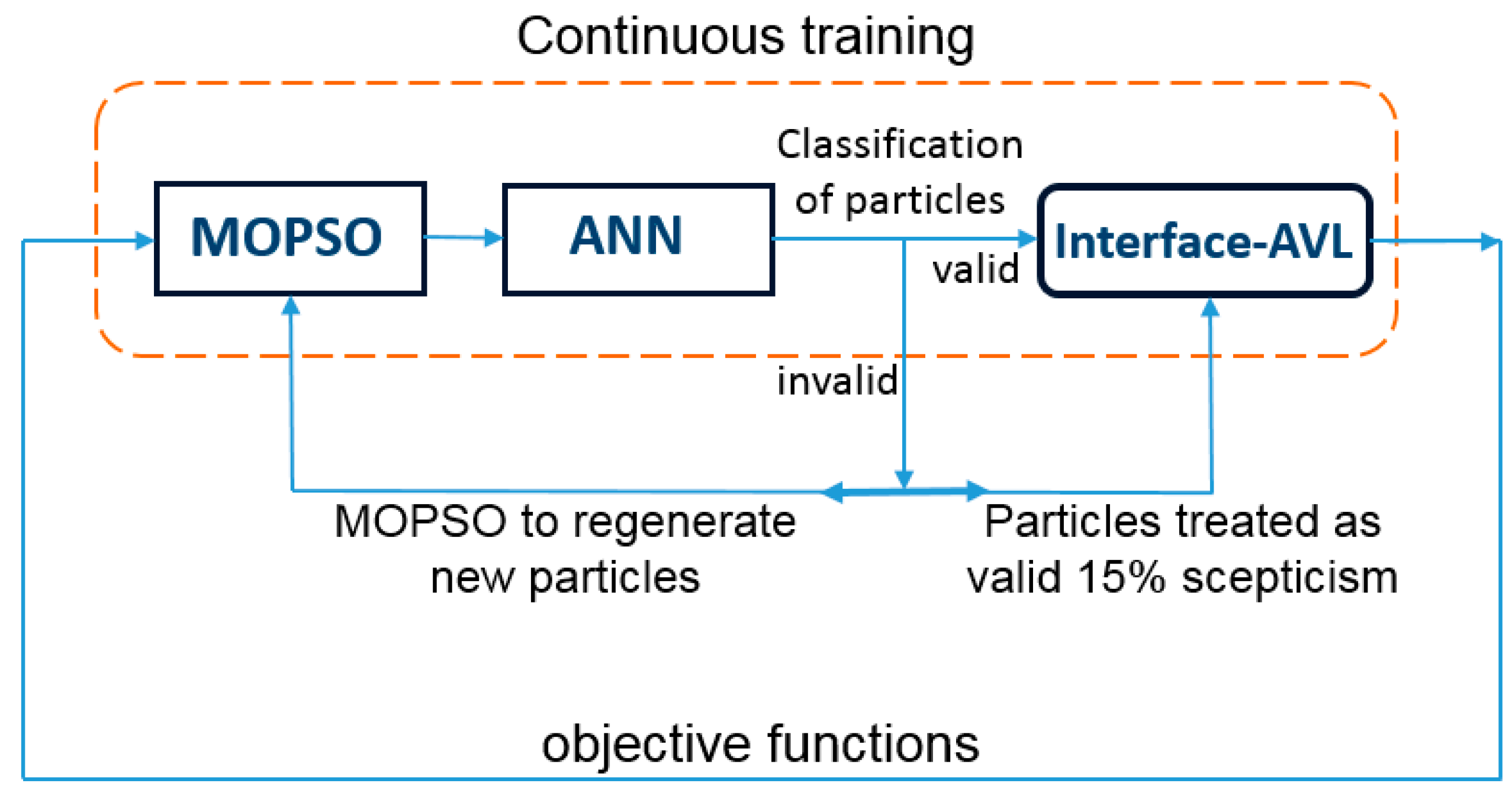
Figure 1 shows the schematic diagram of the proposed ANN framework for the aerodynamic shape design optimisation of the Aegis UAV, obtained by continuous live training and a certain level of scepticism. The scepticism parameter demonstrates the level of doubt towards the invalid solutions that result from the ANN. The learning machine framework consists of three main parts: The Multi-Objective Particle Swarm Optimisation (MOPSO) algorithm, Interface-AVL [43], and the ANN [49]. The optimiser algorithm used in this work was developed and tested by Coello Coello [36,50] to handle multi-objective optimisation design problems, and was inspired by [29]. The majority of MOPSO algorithms share the same basic approach: a swarm of a certain number will be initialized randomly and that number will remain constant until the end of the run. Unlike other proposals of MOPSO, the Coello Coello algorithm has been validated by using several test functions taken from the literature to evaluate multi-objective optimisation. The ANN is used here as a fast approximation evaluator to decide whether the trial solution by the optimiser (MOPSO) is worth full evaluation or not [5]. The flow solver used to evaluate worthwhile solutions is the Athena Vortex Lattice (AVL) [51,52]. Many codes utilize Vortex Lattice Method (VLM) for aerodynamic characteristics calculations, but AVL is the most well-known and provides the most accurate and efficient results when compared with other aerodynamic analysis software employing the same method [45,46,47,48,52]. In addition, AVL code is easy to use and capable of manipulating a large number of design parameters within a short computational time and limited cost. It has the capability to simulate many surfaces at the same time, i.e., the wing downwash effect on the tail, and fuselage wing-tail effect, and to simulate complicated configurations. AVL is most appropriate for UAV configurations, which are comprised of thin lifting surfaces with a small angle of attack [51]. To continuously read the new design variables and then construct the required files for the AVL code, the Interface-AVL code was developed for automatic reading and filing [43]. However, only the solutions signalled by the ANN as valid are modelled for evaluation. Since the AVL code is capable of evaluating only inviscid drag, empirical formulas, commonly called “build-up technique” are used to evaluate zero lift drag. The majority of the equations used in this technique are based on data gathered from flight tests and wind tunnel experiments [53]. To integrate the Interface-AVL with the ANN-MOPSO framework [5], the framework was amended following Tilocca [54]. It was used effectively to define the structure of the input file required by the Interface-AVL. Once the required input files were prepared, the experiment was starting by typing a command in the command line. It was permitted to select the number of particles (swarm), number of iterations, training procedure, and scepticism percentage.
When using a continuous live training approach for the ANN, the trial solutions suggested by the optimiser will be classified by the ANN as valid or invalid. The continuous live training of the ANN was performed in parallel with the evaluation of the objective function by the Interface-AVL. With live training, as used in this work, the training data were gathered and archived by the optimiser while the run was in progress. The minimum size of the training set to be provided for the ANN before starting classification was defined as 500. Then, as the run continued, the ANN classified the trial solutions as valid or invalid. If the ANN classified a trial solution as valid, the corresponding objective function was calculated. When the trial solutions were classified as invalid by the ANN, two different actions were performed. First, 15% (scepticism level) of the invalid particles were treated as a valid particles and sent by the MOPSO to the Interface-AVL to be evaluated. The second action was the recalculations of position and velocity for the other invalid particles which were sent back to the ANN for testing before evaluation. By doing this, the computational time was used only for evaluating the trial solutions accepted by the ANN, whereas the solutions rejected by the ANN wee regenerated by the optimiser as new trial solutions with new velocities and positions. More details about various training processes and other issues regarding the ANN that had a significant effect on the optimisation performance can be found in Section 3.
Overview of the Artificial Neural Network
This work used the ANN as described in [5], and which ran in parallel with the MOPSO. It was an ANN with multilayer perceptron composed of 100 hidden neural layers, each with 10 hidden nodes. The code was originally written in C++, which used the C++ library to help with the computationally intensive tasks [49]. However, to simplify the development of the tool, the interfacing layers were written in Python. Most developments for the tool were for Python script layers, to avoid the core layer which is written in C++ [55]. Python is one of the most popular high-level languages, it contains a wide-ranging library that can be used in machine learning, data mining, and other scientific applications [56]. The ANN remains under active development by the authors, as many researchers have been able to improve this tool by adding new functions to suit their work [55].
For the learning process, the ANN used a limited memory Broyden Fletcher Goldfarb Shanno (L-BFGS) algorithm [5]. This is a straightforward self-optimisation method than can accelerate the pre-training process using a line search method. The L-BFGS algorithm used parallelism for computing the gradients on Central Processing Units (CPUs), Graphics Processing Units (GPUs), and computer clusters [57]. Generally, L-BFGS methods do not require manual tuning for the optimiser parameters to find a good convergence rate and so are considered stable and easy to use for training purposes.
3. Training of the ANN
The capability of the ANN to learn from a set of data that expresses model behaviour is one of its most useful features. Once the ANN has learned the existing relationship between input and output, it can generalise a solution which, in our case, means that the ANN can decide whether the trial solution by the optimiser (MOPSO) is worthy of full evaluation or not.
Various training processes and other issues regarding the ANN that have a significant effect on the optimisation performance are discussed below.
3.1. Initial Training Versus Live Training
Initial training means that the ANN will be trained from existing data. The archive should be prepared in advance so it can be used from an early stage of the optimisation. Using a well-distributed training archive can lead to bad particles being discerned very early, but compiling such a training archive is not always easy and is often expensive, especially for complex industrial problems. In contrast, with live training, as used in this work, the training data can be gathered and archived by the optimiser during the run in progress. When using live training, the decision must be made whether to use single or continuous training.
3.2. Continuous Training Versus Single Training
When doing live training, a consideration that has a significant influence on the optimisation performance is whether to spend all the optimisation time for retraining the ANN or to be satisfied with a shorter period of training and then use this archive of trained data to guide the optimisation until the end. Rawlins et al. [5] argued that time used to train the ANN after each iteration is negligible when compared to the time required for the evaluation of the objective function for the problem. However, continuous training may lead to overtraining that may not provide any further improvement in the predictive ability of an ANN. Thus, it is desirable, if possible, to stop training once an acceptable size for the training archive has been reached.
Real-world problems and especially aerodynamic shape optimisation problems are highly constrained, and that is reflected in their being difficult to solve [6,7]. Thus, aerodynamic shape optimisation usually has many more invalid solutions than valid. For such design problems, using machine learning with continuous training is more efficient than using single training, especially with the knowledge that the time used to train the ANN after each iteration in continuous training is negligible when it is compared to the cost of solving the objective functions [5].
3.3. Size of the Training Set
The definition of the initial training set depends on the training approach adopted by the optimiser. If the training uses a pre-existing archive, the initial training set is the size of sample data drawn from the archive to train the ANN. On the other hand, for single live training, it is the acceptable size of the training set acquired by the optimiser.
In contrast, the size of the training set in the case of continuous training is considered to be the minimum size from the training archive necessary as a reliable source for training. In this research, the minimum size of the training set to be gained by the ANN before commencing classification is defined as 500, see Section 4.4.
3.4. Level of Scepticism
The level of scepticism represents the level of suspicion that we have towards the particles that have been classified as invalid by the ANN. It depends mainly on the size of the archive and whether the training is single or continuous. For this work, 15% was selected, which is appropriate when using a large training set or continuous training approach (to avoid overtraining) [5].
4. Problem Architecture
This section presents the Aegis UAV case study and conditions to be analysed to demonstrate the effectiveness of the proposed methodology. The existing Aegis UAV platform was used with the motivation of developing an approach that can be used for any aircraft, to provide support during the development of the methodology using the available database.
The existing aerodynamic and mass data for the Aegis UAV platform presently in the Aerospace Integration Research Center (AIRC) Laboratory at Cranfield University was used as a continuous feedback to assist in developing the current methodology. The previously obtained in-flight data were computed using the Engineering Sciences Data Unit (ESDU) [58].
4.1. Problem Definition
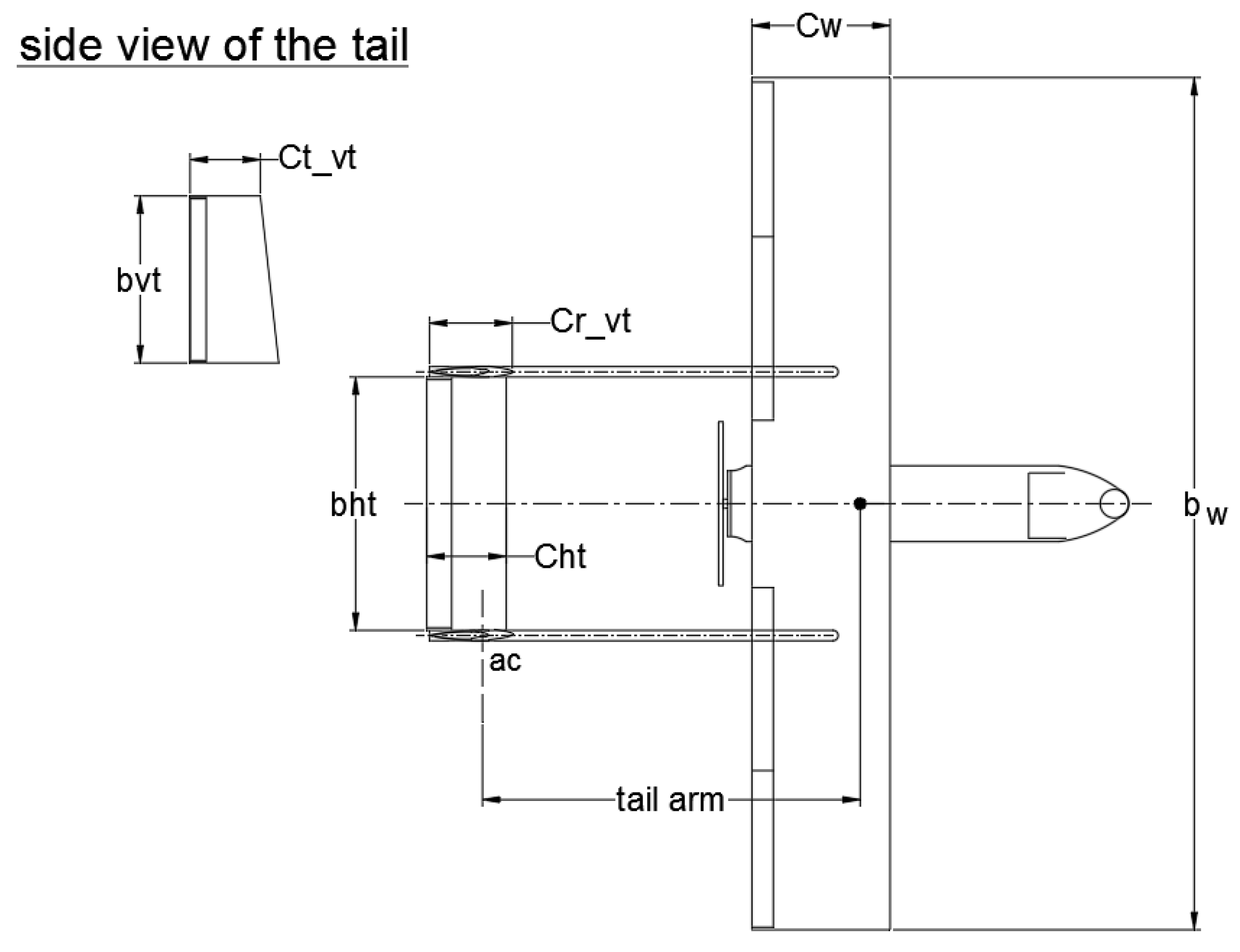
The efficiency and reliability of the proposed methodology have been demonstrated through the aerodynamic shape design optimisation of the Aegis UAV by including wing and tail design variables simultaneously. Figure 2 shows the Aegis UAV configuration with a U-tail shape, where is the wingspan, is the wing chord, and are the horizontal tail span and horizontal tail chord, respectively, is the vertical tail span, is the aerodynamic center, and are the vertical tail tip and the vertical tail root, respectively.
The base values of the design variables shown in Figure 2, with their upper and lower bounds, are listed in Table 1.
The Aegis UAV is still under development by a team from Cranfield University as part of the ATHENA project [58,59]. Formulation of the design problem, defining the design space and the objective functions was done in [43]. Two different objectives were included, to minimise both the endurance ratio [60,61,62] and structural mass , subject to a lift coefficient constant at cruise speed equal of 43.60 m/s (Mach number around 0.13). For level flight this is a single point optimisation problem. Ideally, the design process invariably starts with a shape to satisfy the aerodynamic constraints, and this is followed by adapting the shape to meet the requirements of the other disciplines [63].
The endurance ratio will be optimised using suitable flight conditions (only velocity will be varied) and the design variables [60,61,62]. The optimiser is seeking to minimize the drag coefficient () by varying the shape design variables, subject to . The is the base design lift coefficient. The total mass of the UAV is the sum of the masses of all the subsystems, including the frame structure, propulsion system and payloads, and is parameterized in terms of aircraft wing, boom, and tail design variables. The operational altitude for the UAV is around 2000 m. Based on the wing chord the Reynolds number is around 1.5 × 10⁶.
4.2. Formulation of the Optimisation Problem
We performed an optimisation in which wing-tail design variables were used simultaneously to optimise the Aegis UAV with the U-tail shape. Nine design variables were used to optimise the Aegis UAV with U-tail shape; wing span (), wing root (), wing taper ratio (), horizontal tail volume (), vertical tail volume (), tail arm (), horizontal tail aspect ratio (), vertical tail aspect ratio (), and vertical tail taper ratio (), see Table 1. The formulation of the design problem was as follows:
Here, is the scalar objective function, is the vector of components, and are the lower and upper bounds on each of the design variables, respectively, and are the optimised UAV stall and maximum velocity, respectively, and are the base design stall and maximum velocity, respectively, is the pitching moment coefficient, is the horizontal tail span, is the vertical tail tip, is a pitching moment slip, and are the variation of rolling and yawing force coefficient with sideslip angle, respectively, is a variation of pitching moment coefficient with pitch rate, and is the variation of yawing force coefficient with yaw rate. The design variables were subject to the base design pitching moment .
4.3. Related Work
The Aegis UAV design case reported in this paper was obtained by means of automated optimisation using the Nimrod/O tool [64,65,66] for the Aegis UAV with two tail configurations; U-tail and inverted V-tail. This enabled the designer to manipulate various combination of the design variables and better understand different design scenarios [43,44]. The optimisation was performed using the Multi-Objective Tabu Search (MOTS) algorithm [67,68,69], chosen for its suitability for this type of complex aerodynamic design problem [68,70,71]. However, for confirmation, the authors used optimisation results for this design case to be compared with the leading multi-objective Genetic Algorithmic (GA), NSGA-II. Comparison supports the effectiveness of using the MOTS algorithm in such a design problem (see Appendix A). This was achieved using the High-Performance Computer (HPC) at Cranfield University [72]. Since the objective of the research is modelling and aerodynamic design optimisation of the Aegis UAV at the initial stage of design, the flow solver Athena Vortex Lattice (AVL) was used to capture the relevant physical aspects of the problem. High fidelity codes can be used, if required [2,73].
Once a better understanding of the design problem was obtained, the work focused on making the optimisation process faster by using the interactive optimisation described in [44]. The interactive framework used Multi-Objective Particle Swarm Optimisation (MOPSO) algorithm which has been found to be suitable for this type of design problem [7,37,42].
4.4. Design and Setting of the Experiments
In order to perform fair comparisons, the same design variables and their bounds were used; i.e., the same parameters that were used to define the design optimisation problem in the case of interactive optimisation, and the posterior approach [44]. The ANN-MOPSO-AVL interactive framework was installed on a personal computer with i7-6700 CPU processor. Table 1 shows the design variables and their upper and lower bounds used to define the information required by the flow solver.
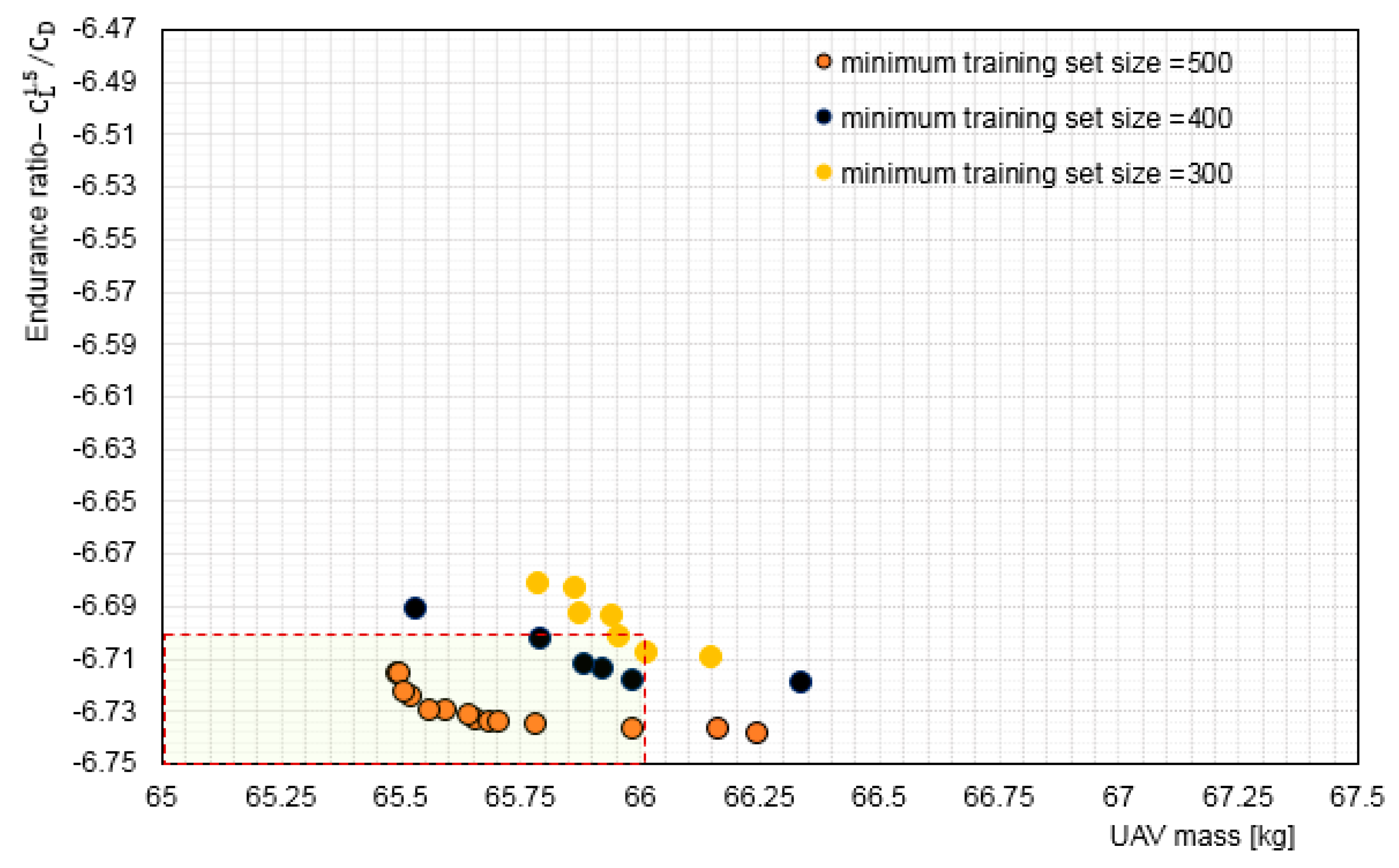
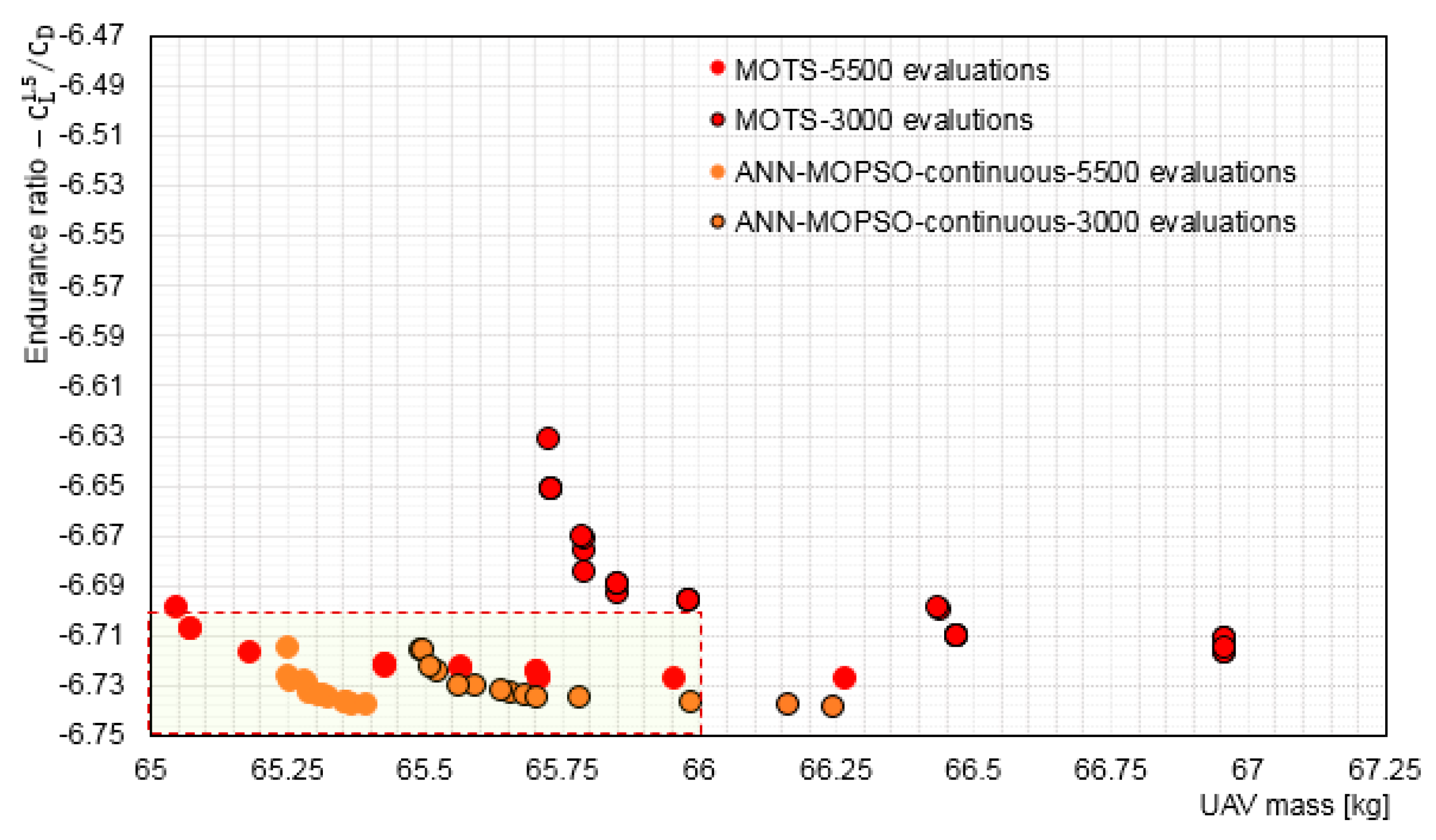
Once the input file was prepared as explained above, the experiment was initiated by typing a command into the command line. In all experiments, the algorithm allowed for 5500 and 3000 objective function evaluations. For the 5500 evaluations, 110 iterations with 50 particles were utilized, and for the 3000 evaluations, 100 iterations with 30 particles. Those are the same parameters used by the experiment in case of the interactive optimisation, which obtained by executing several runs using various combination of iterations and particles. That was very necessary to obtain an assessment of an efficient number of particles and iterations in each run. The continuous live training approach was used for the ANN, and the trial solutions suggested by the optimiser were classified as valid or invalid, as explained in Section 2. Several experiments were performed using training sets of 300, 400 and 500. It can be seen from Figure 3, that a set size of 500 provided significantly better results and it was decided that the minimum training set size for the ANN before starting classification would be 500.
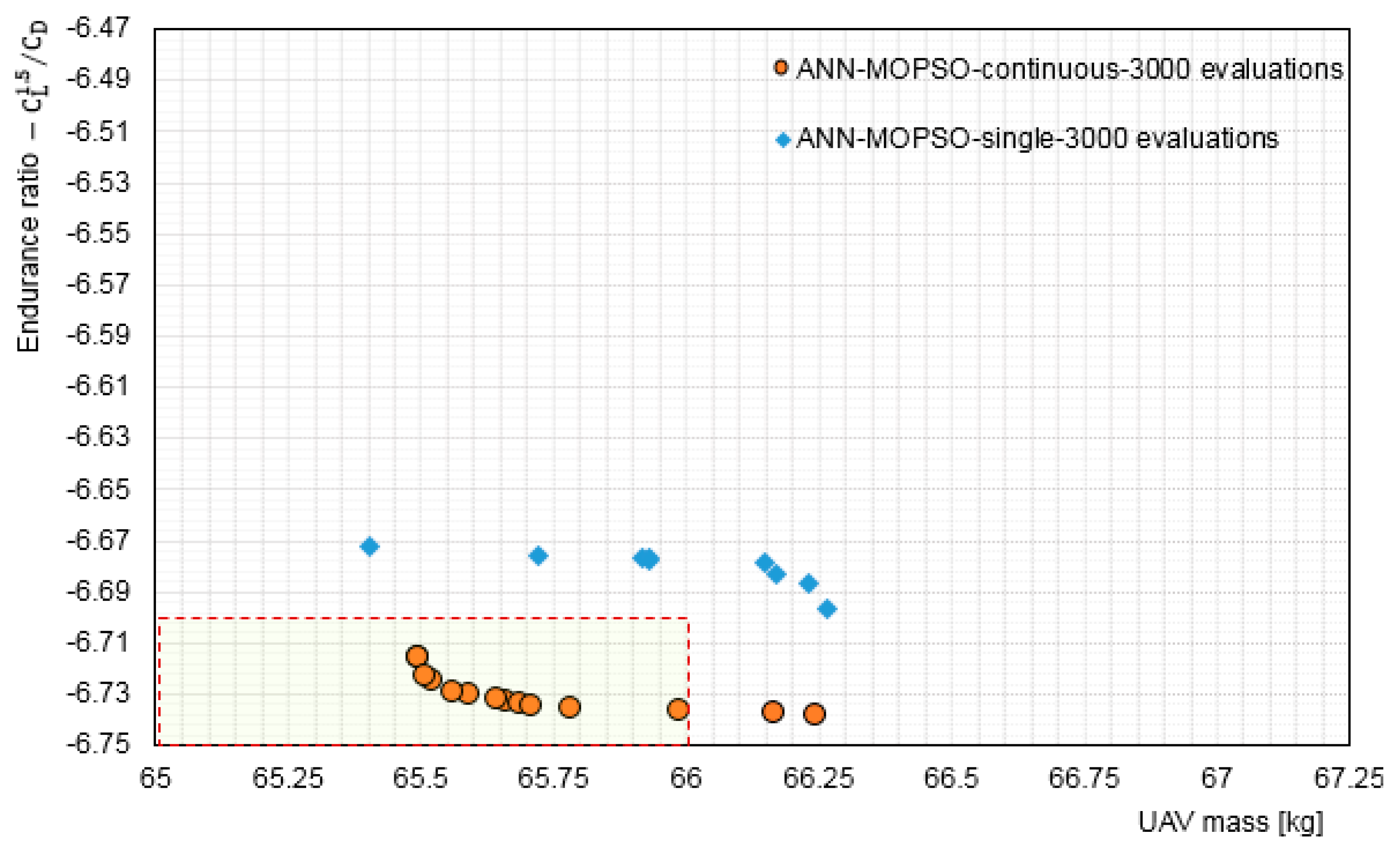
Rawlins et al. [5] have stated that the time consumed by the continuous training of the ANN after each iteration is negligible when compared to the cost of the objective functions. This study carried out several experiments to test this observation by comparing single and continuous training, and the results obtained confirmed Rawlins’ findings. The results showed that continuous training is the better approach for the aerodynamic shape design optimisation problem, see Figure 4. Table 2 summarises the final parameters used in this study.
5. Results, Observations and Discussion
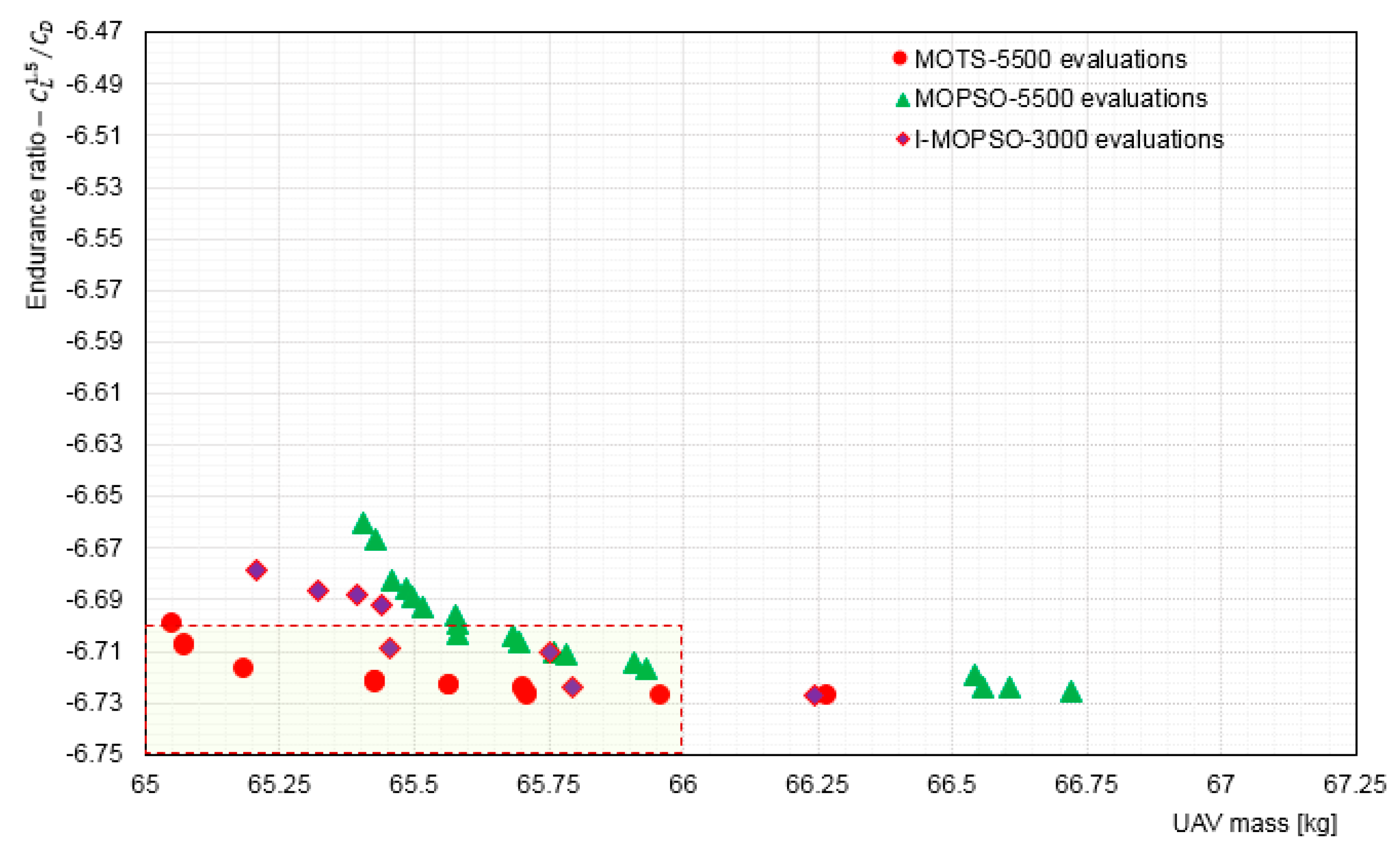
To demonstrate the efficiency and benefit of using the ANN, it was compared to non-interactive and interactive approaches. Figure 5 compares the optimisation results obtained using MOTS and MOPSO for 5500 evaluations with Interactive-Multi-Objective Particle Swarm Optimisation (I-MOPSO) for 3000 evaluations in [44]. It is evident that the DM using only 3000 evaluations was able to guide the optimisation process to within the Region of Interest (ROI).
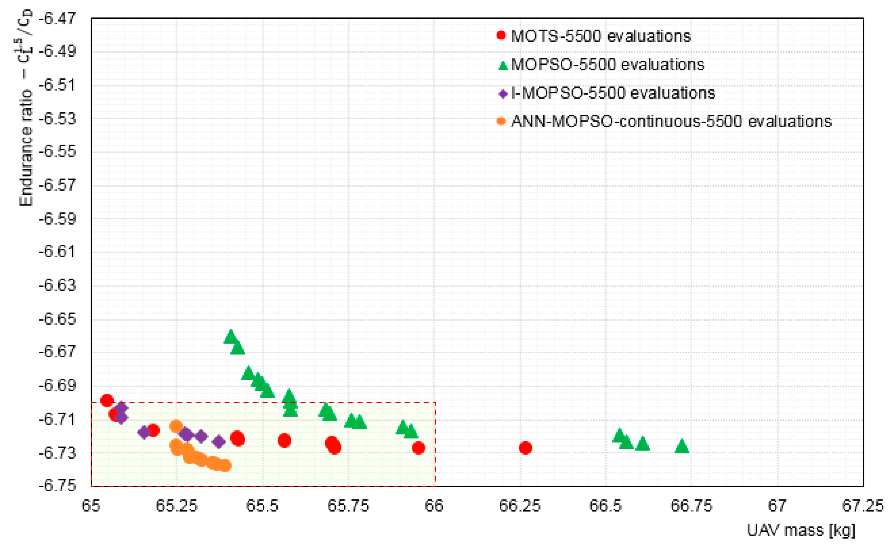
The experiments using the ANN framework started by allowing for 5500 objective function evaluations. The evaluations were divided into sets of 110 iterations and 50 particles. The continuous training approach was selected with a minimum size of training set of 500. Because the algorithm used possesses stochastic characteristics, five-runs were performed. Figure 6 shows a comparison of MOTS, MOPSO, and I-MOPSO with ANN-MOPSO for 5500 evaluations. The results using ANN-MOPSO shows a slightly better improvement by moving towards the centre of the Pareto front. However, some of the MOTS and I-MOPSO solutions obtained a higher reduction in mass than ANN-MOPSO solutions. More analysis was performed using parallel coordinate technique and simulations, and is discussed below.
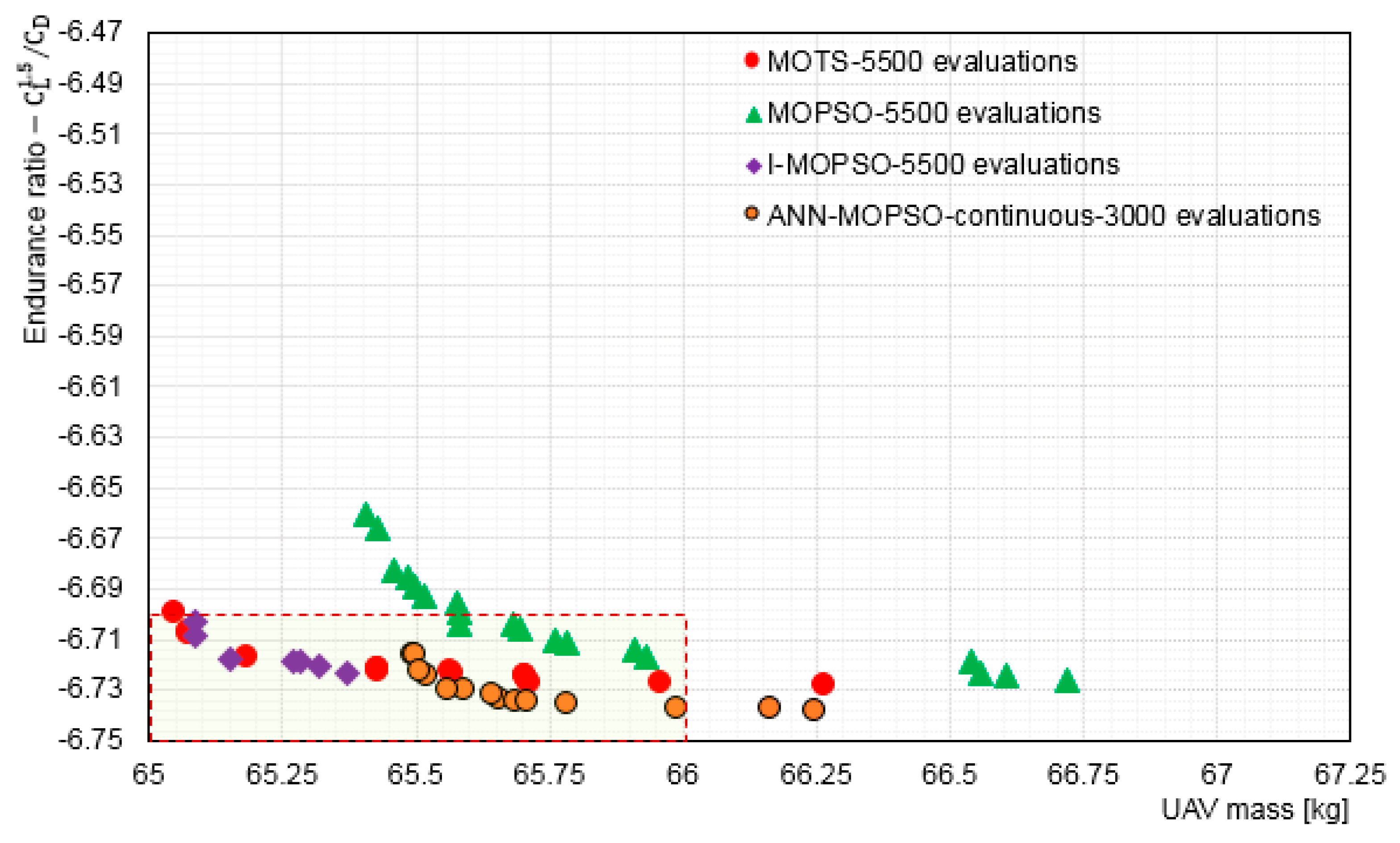
In order to identify the gains in efficiency obtained by using an ANN in the aerodynamic shape design problem, a comparison of ANN-MOPSO results obtained using 3000 evaluations with MOTS, MOPSO, I-MOPSO results obtained for 5500 evaluations is shown in Figure 7. The ANN-MOPSO for 3000 evaluations was able to provide results within the ROI, similar to the optimisation results obtained by MOTS, MOPSO, and I-MOPSO which were for 5500 evaluations. It is evident that by using the ANN the computational time required to obtain results within the ROI is reduced.
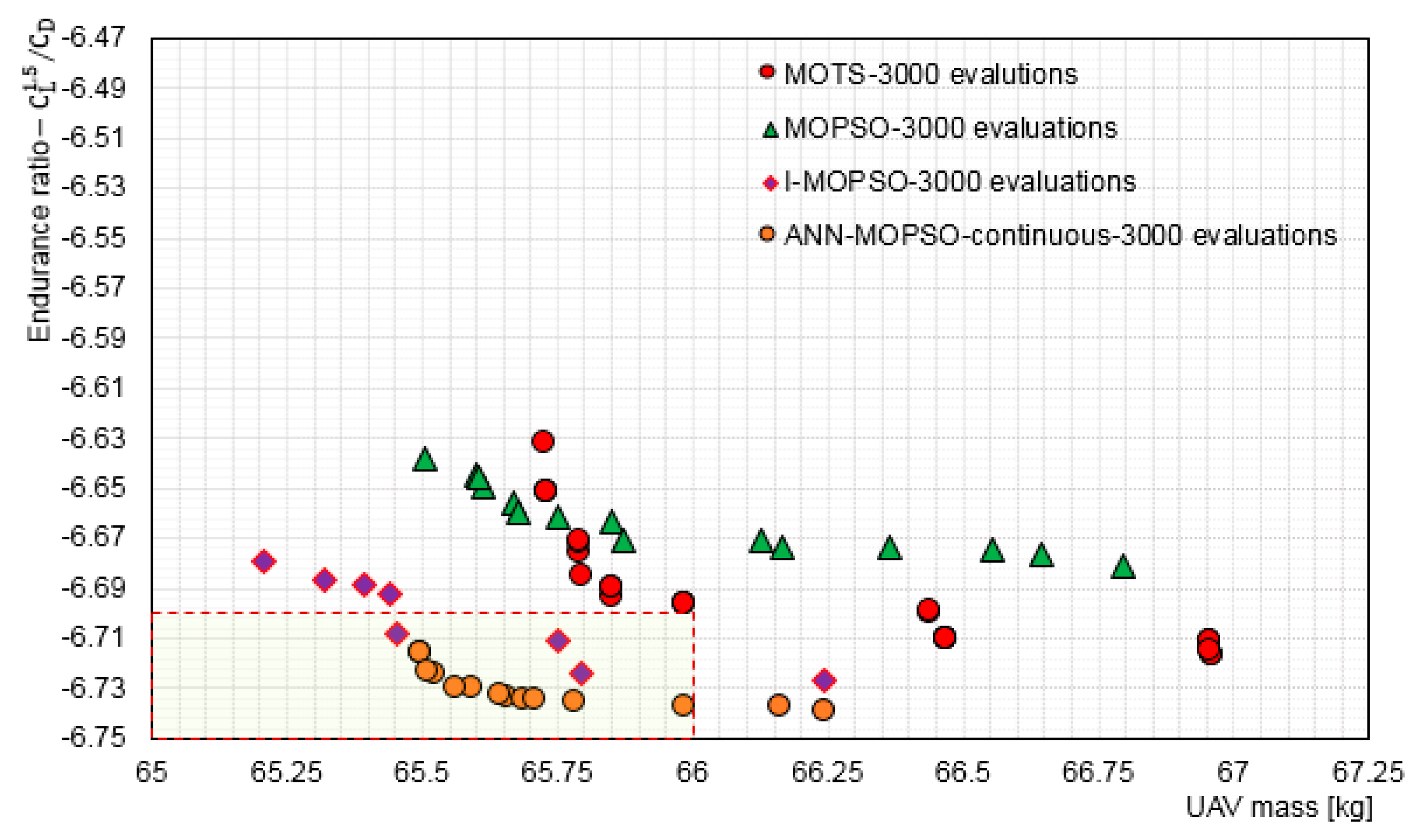
As an additional demonstration of the superiority of using ANN in the optimisation process, a comparison of the results obtained using ANN-MOPSO, MOTS, MOTSO, and I-MOPSO for 3000 evaluations is presented in Figure 8. The superiority of using the ANN to guide the optimisation is obvious. The ANN-MOPSO solutions are better than the interactive results. It is evident that the ANN has efficiently self-trained and succeeded in detecting the invalid particles. This strongly suggests that using an ANN has enabled the optimiser to outperform the other approaches used here. Visual comparison of the Pareto front shows the solutions using an ANN are well inside the ROI and cover both objectives fairly when compared to the solutions obtained using other approaches with the same number of evaluations.
Figure 9 shows a comparison for the simulations using both ANN-MOPSO and MOTS for 5500 and 3000 evaluations. It is clear that as the simulation continues the search it becomes more tightly constrained, and the ANN-MOPSO began facing difficulties in improving the solutions further, which means it had almost reached an optimal solution for this design case. In fact, since the ANN is under continuous training, the exploration regions change smoothly through the generation of new particles in the areas of interest until highly optimal solutions are obtained. The convergence of the solutions towards the centre of the Pareto front is strong evidence of the success achieved by the optimisation search.
Since the ANN is used to guide the optimisation algorithm by detecting invalid particles, it is of interest to display the differences between valid and invalid particles for each approach. Table 3 confirms that the ANN was a significant tool for spotting invalid particles. The results justify the use of an ANN since the DM would have more particles that are valid for almost the same computational time. For example, adding the ANN to MOPSO increased the number of valid particles from 988 to 2238 for 5500 evaluations, and from 529 to 1006 for 3000 evaluations.
It is evident that the ANN is an effective, fast evaluator for deciding if a trial solution passed by the optimiser is worth evaluating or not. Using the ANN-MOPSO improved the number of the valid particles by 126% and 90% compared to the MOPSO alone, but incurring a penalty of 8.0% and 8.3% in computational time, respectively for the 5500 and 3000 evaluations. This time penalty is a small proportion of the time required to evaluate the trial solutions. The difference in computational times is the penalty for using an ANN to classify whether a trial solution is valid or not, for the evaluation and regeneration of new particles by the optimiser. Another finding that demonstrated the efficiency obtained by using the ANN, was that the ANN-MOPSO for 3000 evaluations obtained a higher number of valid particles compared to the MOPSO for 5500 evaluations with significantly less computational time (a 33% reduction—64 min). The number of valid particles was 1006 out of 3000 evaluations obtained using the ANN-MOPSO. In contrast, the number of valid particles was only 988 out of 5500 evaluations when the MOPSO algorithm was used alone. This is a strong indication of the effect of using the ANN for such design problems.
5.1. Data Visualisation and Analysis Using Parallel Coordinates
The Parallel Coordinates (PC) visualisation is a unique tool in the sense that it allows the DM to examine large quantities of data at a glance and quickly focus on the existing correlation, while simultaneously analysing individual measures to derive meaningful insights against the whole. By having a simple glance into the data, the optimisation cases that were able to obtain solutions within the region of interest for the DM are very noticeable. Several visualization techniques are available in the literature [74,75,76], however PC is the most popular [77,78] because it is easy to use and enables the DM to perform tasks interactively and efficiently. One of the earliest reports of work done using PC as a static user interface is in [79]. Visualization of the population in a high-dimensional objective space presented significant information allowing the DM to trade-off between objectives, assessing the quality of the Pareto front, and helping the DM to express his/her preferences [80]. Figure 10 uses Parallel Coordinates to present and analyse the results for the ANN-MOPSO 3000 evaluations, and highly optimal compromise solutions were obtained. The solution obtained using the ANN-MOPSO 5500 evaluations provided an even better compromise for the objective function.
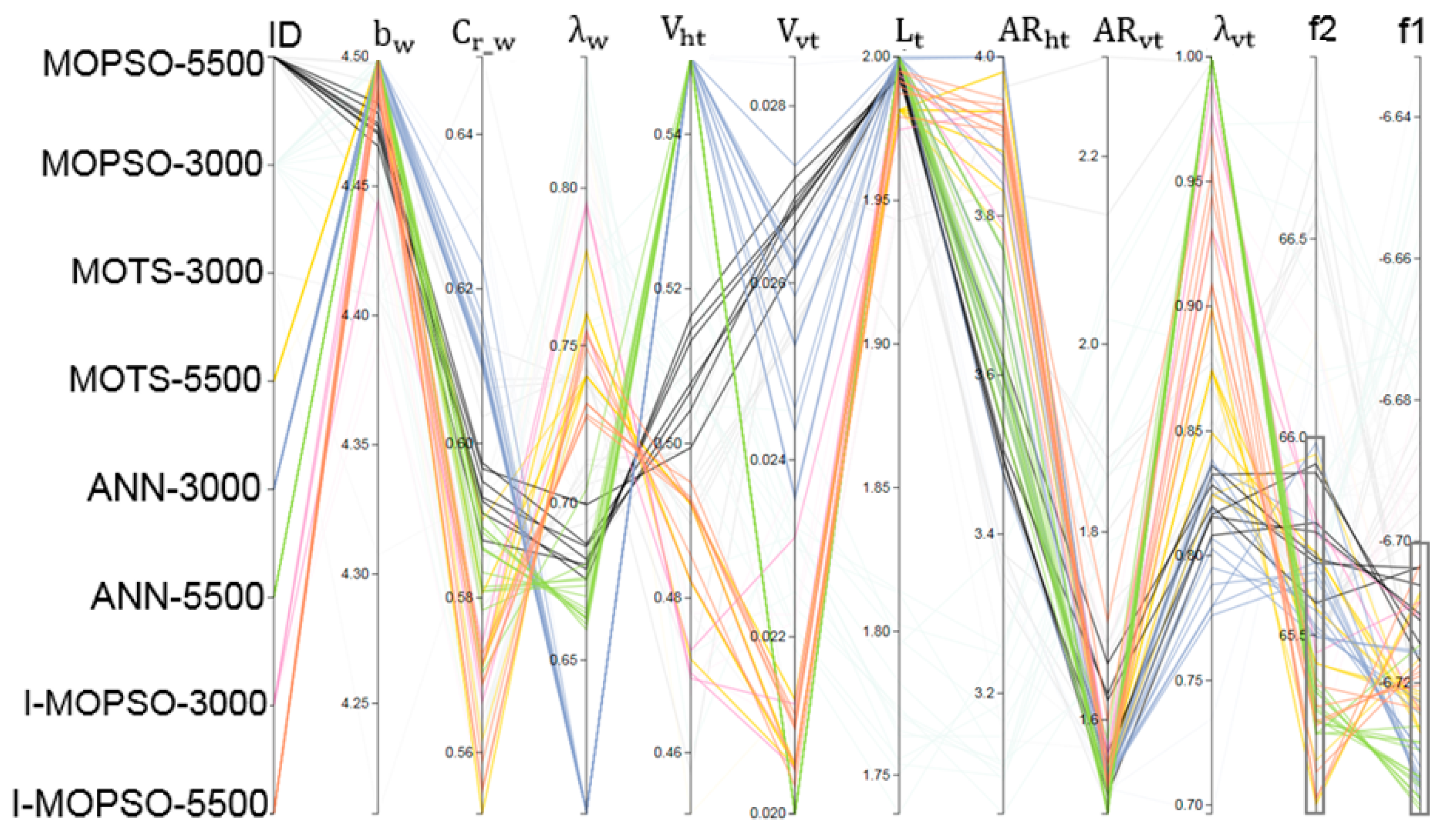
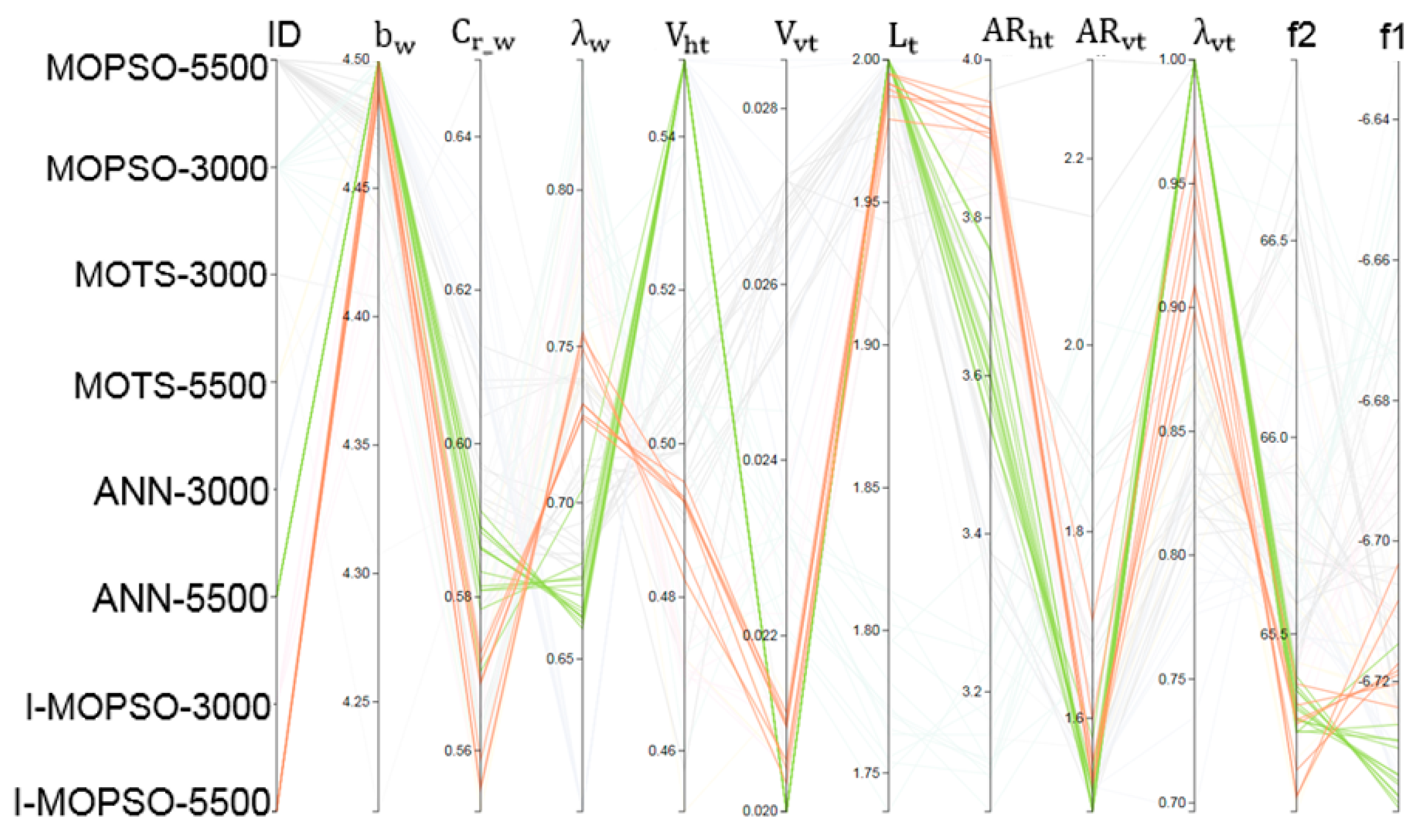
One of the early observations, when visualising the data using parallel coordinate, were the strong correlations obtained when the ANN was used to guide the optimisation process. Study and analysis of these trends revealed correlations between the design variables and objective functions, see Figure 11. It brought to light meaningful multivariate patterns and comparisons that helped when used interactively by the DM for analysis and design preferences. Particularly, it helped with identifying which of the design variables, or combination of design variables, particularly participated in obtaining optimal objective functions, i.e., it brought to the attention of the DM more than one design option that could be suitable for the next stage of the design process. For example, highly optimal solutions for the Aegis UAV were achieved by using almost the maximum value for each of the wing span, horizontal tail volume, and tail arm. Whereas, the wing chord, wing taper ratio, vertical tail volume, horizontal tail aspect ratio and vertical tail aspect ratio should take values around 0.59 m, 0.67, 0.02, 3.6, and 1.5, respectively.
In fact, the optimisation is a complicated process where the optimiser is “playing” with nine design variables, seeking to obtain a set of optimal UAV configurations that satisfies both of the objectives but where, as described earlier, the objectives have conflicting requirements regarding the values of the design variables.
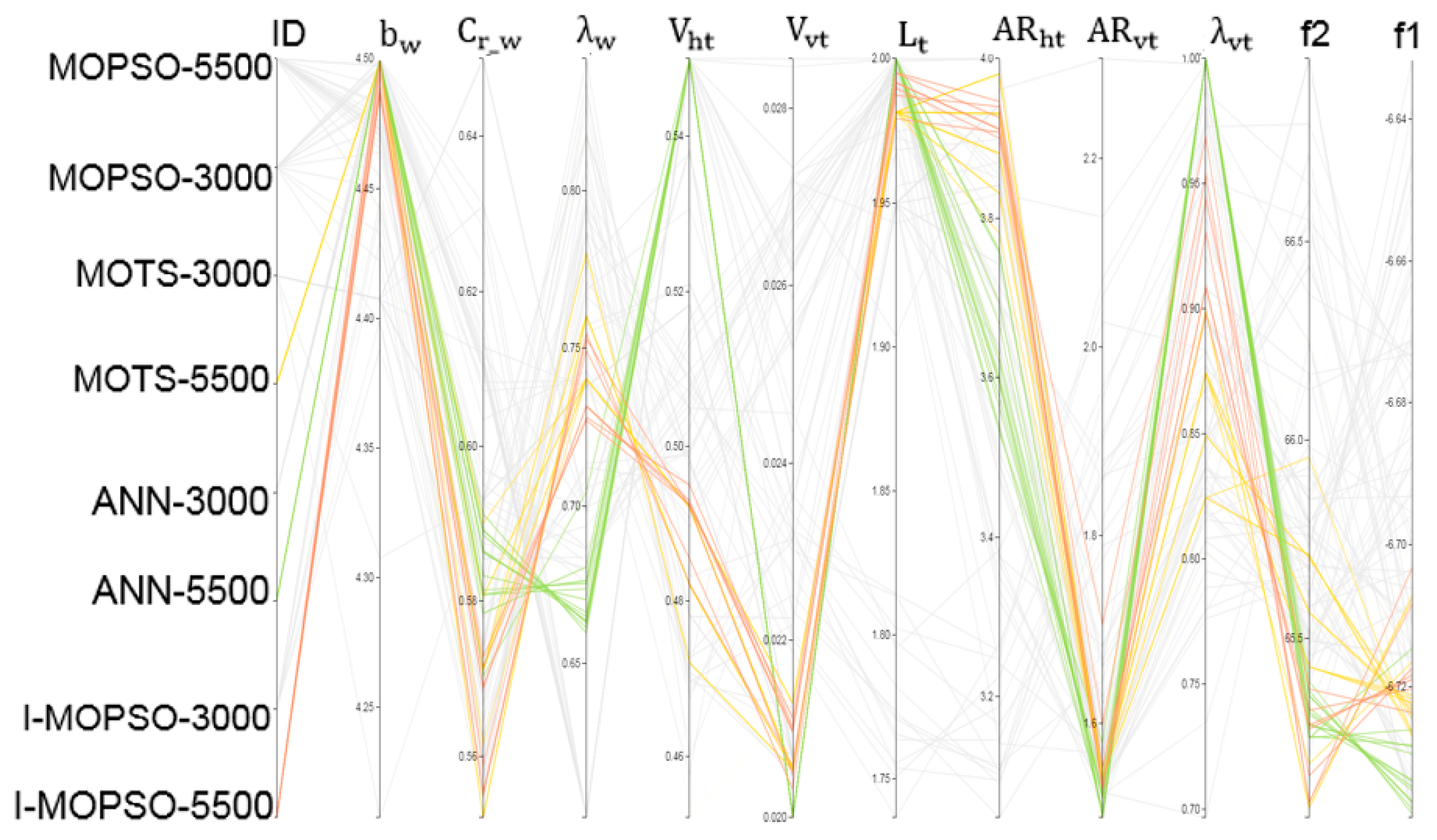
Figure 12 compares solutions obtained for 5500 evaluations using the ANN-MOPSO, MOTS and I-MOPSO algorithms. The solutions obtained using ANN-MOPSO provide the greatest improvement in the endurance ratio, but part of the solution gave less reduction of mass. It is obvious that the ANN solutions significantly minimised the drag by selecting lower wing taper ratio and a higher wingspan. On the other hand, the MOTS and I-MOPSO solutions selected lower values for the wing root chord, vertical tail taper ratio and slightly higher horizontal tail aspect ratio, which resulted in a greater reduction in the mass. However, all solutions satisfied the design requirements, and offer different options for the designer in the next stage. Thus, some design variables can be considered as key for the designer to obtain the required final solution.
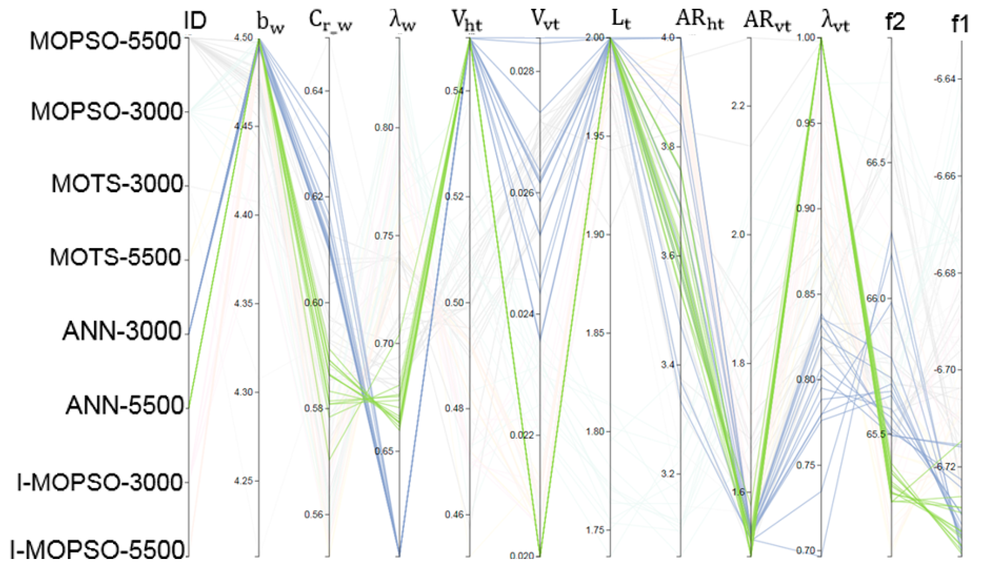
The patterns and correlations obtained using the ANN have an identical trend to the trend achieved by the DM when performing optimisation interactively. Figure 13 compares trends achieved using ANN-MOPSO and I-MOPSO for 5500 evaluations. The similarity in the trends is obvious. These observations highlight the effect of performing optimisation interactively. The correlations achieved by the DM to drive the results are similar to the correlations learned by the ANN to obtain highly optimal solutions.
5.2. Detailed Study for Selected Solutions
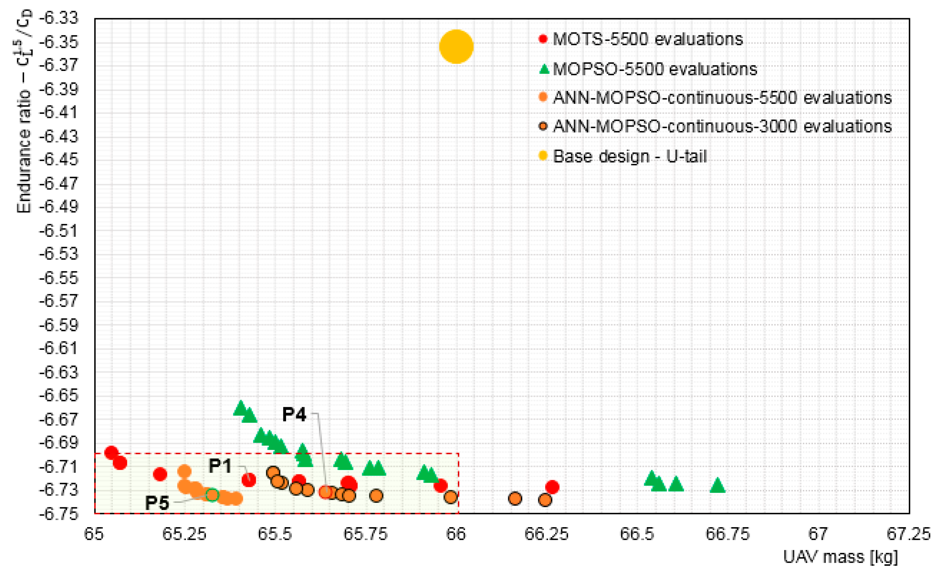
In order to demonstrate the quality of the non-dominated solutions obtained under ANN guidance, a single compromise solution was selected for further simulations. Figure 14 compares optimal compromise solutions obtained using ANN-MOPSO for 5500 and 3000 evaluations, with MOTS and MOPSO for 5500 evaluations, and with the base design. The variations of non-dominated solutions with respect to the objective functions are obvious, giving the DM a deeper insight into the design problem to assist with trade-off.
It is obvious that all the compromise solutions are within the ROI. The compromise solution P5 has the best improvements in both of the objectives compared to the compromise solutions P4 and P1. On the other hand, the compromise solution P4 has better improvement in endurance ratio than P1, but slightly less reduction in mass. However, it must be borne in mind that the compromise solution P4 was obtained after only 3000 evaluations whereas the compromise solutions P5 and P1 were obtained after 5500 evaluations.
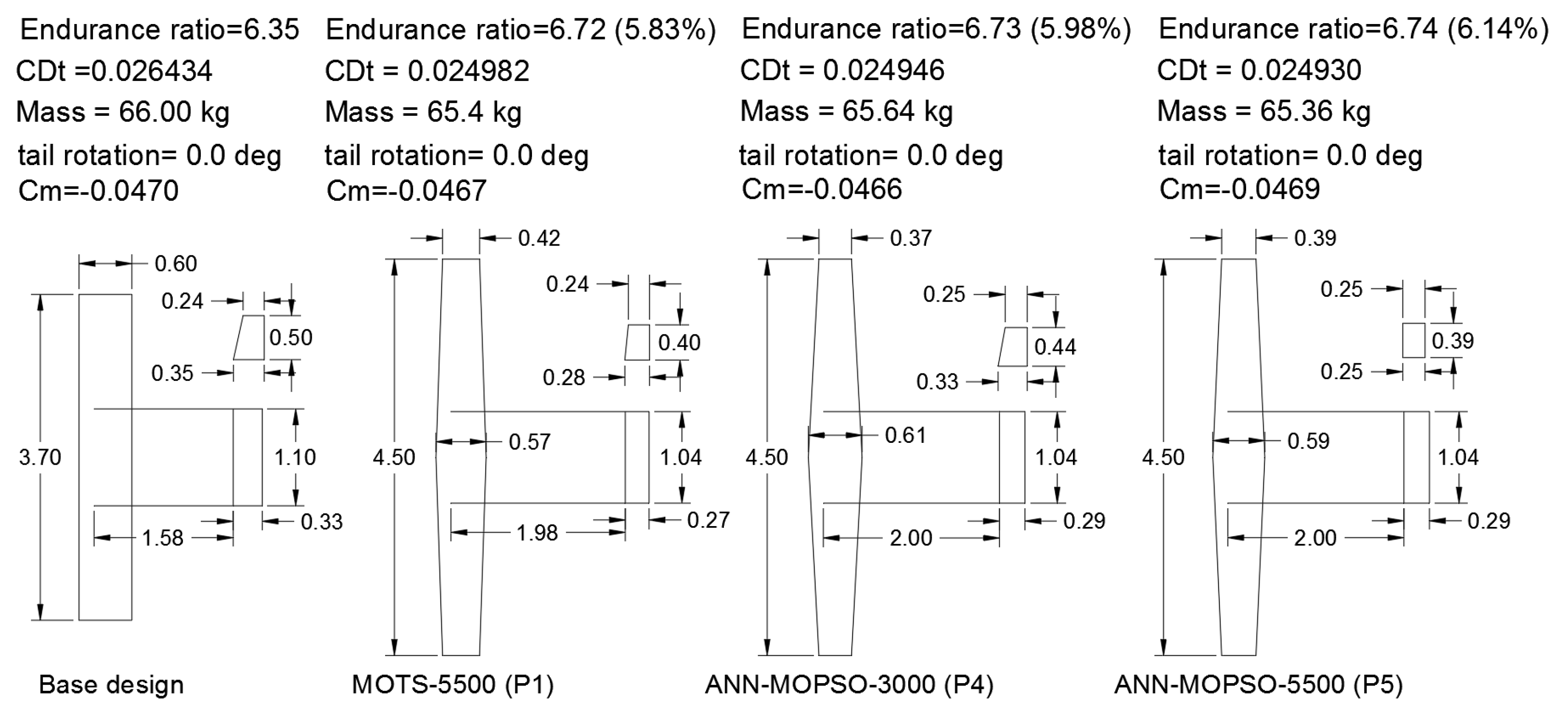
The compromise solution P4 has an endurance ratio of 5.98% higher than that for the base design with 0.55% reduction in mass, whereas the endurance ratio for the compromise solutions P5 and P1 improved by 6.14% and 5.83% with 0.97% and 0.91% reduction in total mass, respectively compared to base design. The drag decreased from 264.3 counts at level flight (for the base design) to 249.3 counts, 249.5 counts, and 249.8 counts, respectively for P5, P4, and P1. Detailed comparison shows that P5 and P4 are 0.52 and 0.36 drag counts lower than P1, respectively. Thus, P5 has the lowest drag value, and P4 has the second lowest drag value, regardless of increasing the number of evaluations.
The drag reduction for the ANN-MOPSO-3000 optimal compromise solution was gained with a decrease in the negative pitching moment when compared to base design and P1, which has a slightly positive effect on release the aircraft from drag increments at trimming, see Figure 15. From these results, we conclude that using an ANN to guide the optimisation by identifying invalid particles is a strong approach. Using only around half of the evaluations (P4), the ANN was able to obtain better results than those obtained using MOPSO and MOTS for 5500 evaluations. The success was due to its ability to better identify invalid particles and hence provide more valid particles in the same computational time.
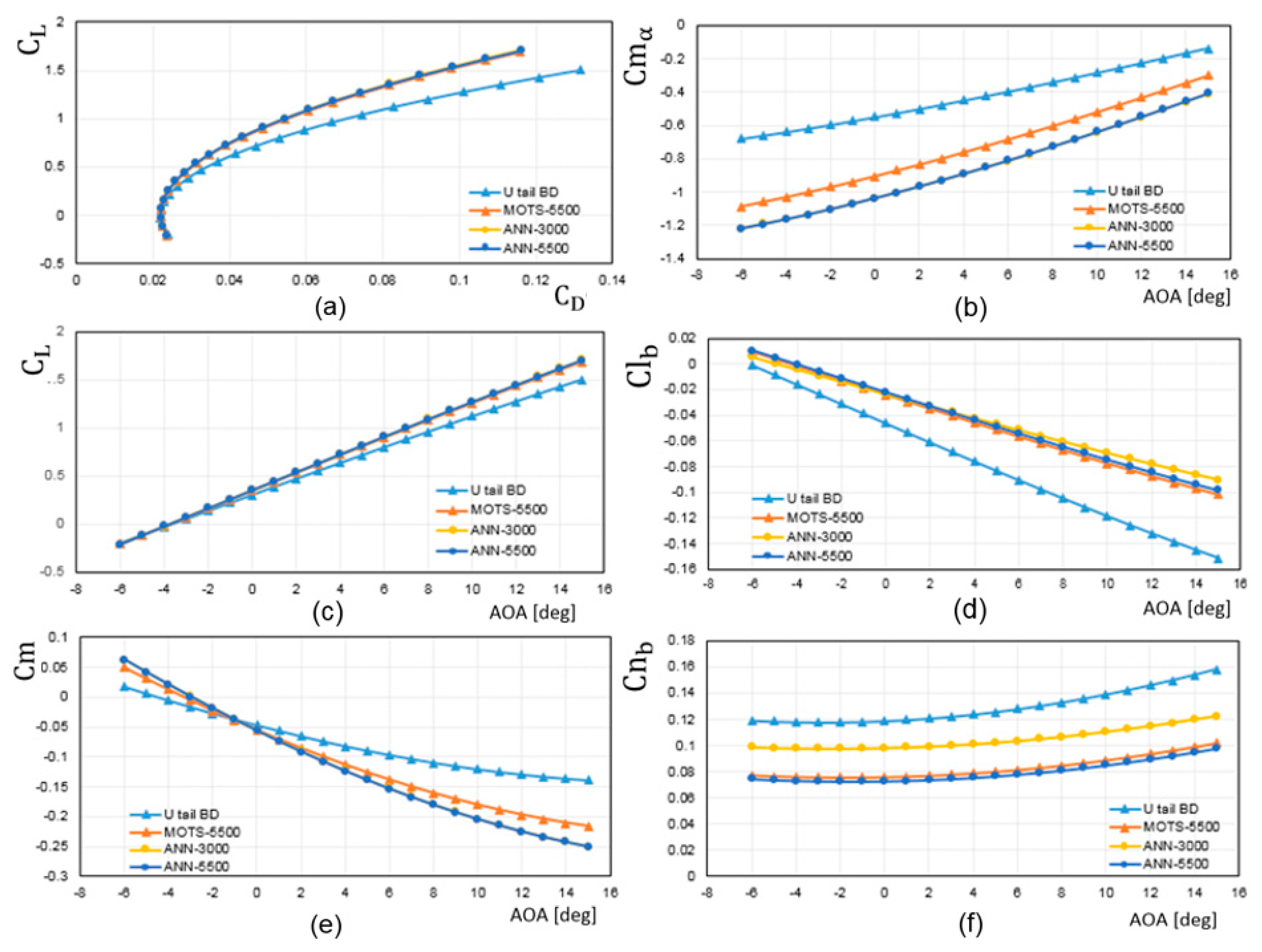
Further investigation is continuing, performing aerodynamic simulations for each of the above configurations as a function of various angles of attack (AOA). Actually, we are most interested in the configuration optimised using the ANN with 3000 evaluations, however the configuration optimised using the ANN with 5500 evaluation is also included. Figure 16 shows a comparison of the aerodynamic characteristics of the selected configurations. It is observed that all the configurations show the same trends. However, as angle of attack increases there will be a positive deviation in lift coefficient, compared to the base design values in the all optimised configurations. Furthermore, the configurations optimised by the guidance of the ANN have a slightly better lift to drag ratio than P1 (optimised using MOTS). On the other hand, there is noticeable variation in stability characteristics for the all optimised configurations even though they satisfy all the design constraints. This behaviour is strongly demonstrated by the dimensions of the optimised configurations. A quick glance at the optimised configurations shows that the optimised configurations had wings with almost the same dimensions whereas there are noticeable differences in the tail dimensions.
It is obvious that the optimiser has reached a stage where no more space is available in the wing design variables to improve the objectives by making changes to the wing planform, whereas there is still more space to play with tail components.
6. Conclusions
This study presents the use of an ANN to aid in optimisation of a multi-objective design problem in order to reduce the workload on the designer by achieving effective solutions. The ANN is used here as a fast approximate evaluator to decide whether the trial solution by the optimiser is worth a full evaluation or not. It was considered proof that the aerodynamic shape optimisation problem is highly constrained and that there are many more invalid solutions than valid. It is not sensible to spend a long time evaluating the non-worthwhile solutions.
The study of the optimisation results showed the success of the ANN in increasing the number of worthwhile particles efficiently. The number of valid particles grew from 988 to 2238 (126%) and from 529 to 1006 (90%), respectively for 5500 and 3000 evaluations using ANN-MOPSO. In addition, the results showed that continuous training is a better approach for the aerodynamic shape design optimisation problem. It is proven that the time used to train the ANN and then identify the invalid particles is small compared to the time for the evaluation of the objective functions. Furthermore, it is evident that by adopting the continuous live training approach, the ANN-MOPSO allows for smooth exploration of the search regions by updated the search continuously when it has not succeeded in improving the solutions by replacing invalid particles with valid particles in regions of interest. That means it helps overcome the drawbacks in the stochastic characteristics of the algorithm, and simultaneously makes it less likely that any important data in the design space will be missed.
The effectiveness of the algorithm is demonstrated by comparing results for the ANN-MOPSO using 3000 evaluations with MOPSO and MOTS for 5500 evaluations and I-MOPSO for 3000 evaluations, subject to the same constraints and design variables. The obtained results strongly indicate that using the ANN to guide the optimisation algorithm is effective at increasing the convergence of the optimiser and obtaining highly optimal solutions. The algorithm incorporating the continuous training approach has been shown to be effective in terms of computational time and solution quality.
In order to increase the efficiency of the framework used, future work could extend and improve the ANN-MOPSO technique, by providing a standard procedure to be followed when selecting training processes and other issues required by the ANN before starting classification of the particles as either valid or invalid.
Author Contributions
Y.A. performed all the simulations and work in this manuscript. A.S. and T.K. provided the guidance and feedback on the results that presented in this paper.
Funding
This research received no external funding.
Conflicts of Interest
The authors declare no conflict of interest.
Appendix A
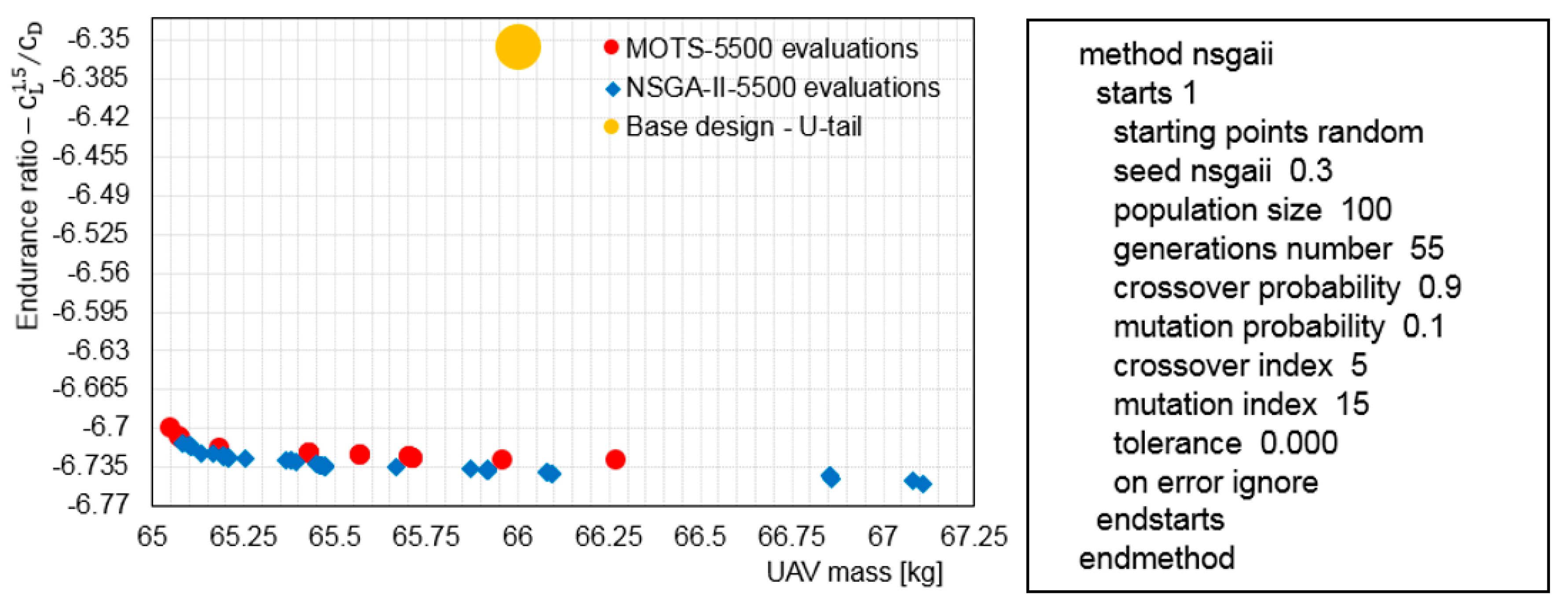
To assess the relative effectiveness of using MOTS for this study, a comparison with the optimisation results obtained by NSGA-II [81] was performed for Aegis UAV design case. Since the NSGA-II algorithm has a non-deterministic behaviour, the results of multiple runs using the same design variables in Aegis UAV case study were collected and assessed. In every case, the experiments were run for 5500 function evaluations. The NSGA-II algorithm used 55 generations for a population size of 100. The left panel of Figure A1 presents the optimisation results obtained using MOTS for 5500 evaluations and NSGA-II also for 5500 evaluations. The right panel of Figure A1 shows the NSGA-II parameter settings.
Figure A1.
Left panel; comparison of the optimisation results obtained using MOTS and NSGA-II for 5500 evaluations: right panel; shows the parameter setting for NSGA-II.
Figure A1.
Left panel; comparison of the optimisation results obtained using MOTS and NSGA-II for 5500 evaluations: right panel; shows the parameter setting for NSGA-II.

It is obvious that both algorithms achieved almost the same quality solutions, but the non-dominated solutions obtained by NSGA-II have greater variance. On the other hand, regardless of the optimisation and search techniques used by each algorithm, the run-times for MOTS and NSGA were 135 and 142 min respectively. This indicates that the MOTS algorithm is slightly more efficient than NSGA-II for such design problems. Overall, the MOTS algorithm exhibited better performance when compared to the leading multi-objective GA, NSGA-II.
References
- Pourbahman, Z.; Hamzeh, A. Reducing the Computational Cost in Multi-objective Evolutionary Algorithms by Filtering Worthless Individuals. arXiv, 2014; arXiv:1401.5808. [Google Scholar]
- Piperni, P.; DeBlois, A.; Henderson, R. Development of a Multilevel Multidisciplinary-Optimization Capability for an Industrial Environment. AIAA J. 2013, 51, 2335–2352. [Google Scholar] [CrossRef]
- Zhang, M.; Jungo, A.; Gastaldi, A.; Melin, T. Aircraft Geometry and Meshing with Common Language Schema CPACS for Variable-Fidelity MDO Applications. Aerospace 2018, 5, 47. [Google Scholar] [CrossRef]
- Viúdez-Moreiras, D. Performance influences on metamodelling for aerodynamic surrogate-based optimization of an aerofoil. Eng. Optim. 2019, 51, 427–446. [Google Scholar] [CrossRef]
- Rawlins, T.; Lewis, A.; Hettenhausen, J.; Kipouros, T. Enhancing MOPSO through the guidance of ANNs. In Proceedings of the International Joint Conference on Neural Networks (IJCNN), Beijing, China, 6–11 July 2014; pp. 4003–4010. [Google Scholar] [CrossRef]
- Kenway, G.K.; Mishra, A.; Secco, N.R.; Duraisamy, K.; Martins, J. An Efficient Parallel Overset Method for Aerodynamic Shape Optimization. In Proceedings of the 58th AIAA/ASCE/AHS/ASC Structures, Structural Dynamics, and Materials Conference, Grapevine, TX, USA, 9–13 January 2017. [Google Scholar] [CrossRef]
- Zapotecas Martinez, S.; Arias Montano, A.; Coello Coello, C.A. Constrained Multi-objective Aerodynamic Shape Optimization via Swarm Intelligence. In Proceedings of the 2014 Annual Conference on Genetic and Evolutionary Computation, Vancouver, BC, Canada, 12–16 July 2014; pp. 81–88. [Google Scholar] [CrossRef]
- Jyoti, S.K.; Manjusha, K.D.; Pavan, K.D. Review on Computing Machinery and Intelligence. Int. J. Curr. Microbiol. Appl. Sci. 2018, 7, 442–451. [Google Scholar]
- Kotsiantis, S.B. Supervised Machine Learning: A Review of Classification Techniques. Informatica 2007, 31, 249–268. [Google Scholar] [CrossRef]
- Mair, C.; Kadoda, G.; Le, M.; Phalp, K.; Scho, C.; Shepperd, M.; Webster, S. An investigation of machine learning based prediction systems. J. Syst. Softw. 2000, 53, 23–29. [Google Scholar] [CrossRef]
- Jordan, M.; Kleinberg, J.; Scho, B. Pattern Recognition and Machine Learning; Microsoft; Springer: New York, NY, USA, 2006; ISBN 9780387310732. [Google Scholar]
- Chen, F.; Li, H.; Xu, Z.; Hou, S.; Yang, D. User-friendly optimization approach of fed-batch fermentation conditions for the production of iturin A using artificial neural networks and support vector machine. Electron. J. Biotechnol. 2015, 18, 273–280. [Google Scholar] [CrossRef]
- Mekky, A.; Alberts, T.E. Design of a Stochastic Basis Function Artificial Neural Network Controller for Quadrotors Flight in the Presence of Model and Aerodynamic Uncertainties. In Proceedings of the EEE National Aerospace and Electronics Conference, Dayton, OH, USA, 23–26 July 2018; pp. 395–402. [Google Scholar] [CrossRef]
- Giannakoglou, K.C.; Papadimitriou, D.I.; Kampolis, I.C. Aerodynamic shape design using evolutionary algorithms and new gradient-assisted metamodels. Comput. Methods Appl. Mech. Eng. 2006, 195, 6312–6329. [Google Scholar] [CrossRef]
- Peng, H.; Ling, X. Optimal design approach for the plate-fin heat exchangers using neural networks cooperated with genetic algorithms. Appl. Therm. Eng. 2008, 28, 642–650. [Google Scholar] [CrossRef]
- Amirian, E.; John Chen, Z. Cognitive Data-Driven Proxy Modeling for Performance Forecasting of Waterflooding Process. Glob. J. Technol. Optim. 2017, 8, 1–9. [Google Scholar] [CrossRef]
- Kuo, R.J.; Chi, S.C.; Kao, S.S. A decision support system for selecting convenience store location through integration of fuzzy AHP and artificial neural network. Comput. Ind. 2002, 47, 199–214. [Google Scholar] [CrossRef]
- Cilla, M.; Borgiani, E.; Martínez, J.; Duda, G.N.; Checa, S. Machine learning techniques for the optimization of joint replacements: Application to a short-stem hip implant. PLoS ONE 2017, 12, 1–16. [Google Scholar] [CrossRef] [PubMed]
- Rai, M.M.; Field, M. Robust Optimal Aerodynamic Design Using Evolutionary Methods and Neural Networks. In Proceedings of the 42nd AIAA Aerospace Sciences Meeting and Exhibit, Aerospace Sciences Meetings, Reno, NV, USA, 5–8 January 2004; pp. 1–27. [Google Scholar]
- Askarzadeh, A.; Rezazadeh, A. Artificial neural network training using a new efficient optimization algorithm. Appl. Soft Comput. J. 2013, 13, 1206–1213. [Google Scholar] [CrossRef]
- Volume, C.E.; Electrical, A.; Engineering, A. Redesign of Morphing UAV for Simultaneous Improvement of Directional Stability and Maximum Lift/Drag Ratio. Adv. Electr. Comput. Eng. 2018, 18, 57–62. [Google Scholar]
- Boutemedjet, A.; Samardžić, M.; Rebhi, L.; Rajić, Z.; Mouada, T. UAV aerodynamic design involving genetic algorithm and artificial neural network for wing preliminary computation. Aerosp. Sci. Technol. 2019, 84, 464–483. [Google Scholar] [CrossRef]
- Rai, M.M. Three-Dimensional Aerodynamic Design Using Artificial Neural Networks. In Proceedings of the 40th AIAA Aerospace Sciences Meeting & Exhibit, Reno, NV, USA, 14–17 January 2002. [Google Scholar]
- Rai, M.M.; Madavan, N.K. Aerodynamic design using Neural Networks. AIAA J. 2000, 38, 173–182. [Google Scholar] [CrossRef]
- Mukesh, R.; Lingadurai, K.; Selvakumar, U. Airfoil Shape Optimization based on Surrogate Model. J. Inst. Eng. Ser. C 2017, 99, 1–8. [Google Scholar] [CrossRef]
- Duchaine, F.; Gicquel, L.Y.M.; Bissières, D.; Bérat, C.; Poinsot, T. Automatic Design Optimization Applied to Lean Premixed Combustor Cooling. Available online: https://scholar.google.co.uk/scholar?hl=en&as_sdt=0%2C5&q=Automatic+Design+Optimization+Applied+to+Lean+Premixed+Combustor+Cooling&btnG= (accessed on 15 June 2018).
- Rao, R.V.; Rai, D.P.; Balic, J. A multi-objective algorithm for optimization of modern machining processes. Eng. Appl. Artif. Intell. 2017, 61, 103–125. [Google Scholar] [CrossRef]
- Muhtar, A.; Mustika, I.W. The Comparison of ANN-BP and ANN-PSO as Learning Algorithm to Track MPP in PV System. In Proceedings of the 7th International Annual Engineering Seminar (InAES), Yogyakarta, Indonesia, 1–2 August 2017; pp. 1–6. [Google Scholar]
- Poli, R.; Kennedy, J.; Blackwell, T. Particle swarm optimization. In Proceedings of the IEEE International Conference on Neural Network, Perth, Australia, 27 November–1 December 1995; Volume 4, pp. 1942–1948. [Google Scholar]
- Salomon, R. Evolutionary Algorithms and Gradient Search: Similarities and Differences. IEEE Trans. Evol. Comput. 1998, 2, 45–55. [Google Scholar] [CrossRef]
- Sa, P.K.; Sahoo, M.N.; Murugappan, M.; Wu, Y.; Majhi, B. Progress in Intelligent Computing Techniques: Theory, Practice, and Applications; Springer: Singapore, 2016. [Google Scholar]
- Ebrahimi, M.; Jahangirian, A. Accelerating global optimization of aerodynamic shapes using a new surrogate-assisted parallel genetic algorithm. Eng. Optim. 2017, 49, 2079–2094. [Google Scholar] [CrossRef]
- Annicchiarico, W. Metamodel-assisted distributed genetic algorithms applied to structural shape optimization problems. Eng. Optim. 2007, 39, 757–772. [Google Scholar] [CrossRef]
- Verma, H.O.; Peyada, N.K.; Singh, S. Aerodynamic Modelling of Quasi Steady Stall Using Neural-Network Based Gauss Newton Method. In Proceedings of the International Conference on Infocom Technologies and Unmanned Systems (Trends and Future Directions) (ICTUS), Dubai, UAE, 18–20 December 2017. [Google Scholar]
- Magrini, A.; Benini, E. Aerodynamic Optimization of a Morphing Leading Edge Airfoil with a Constant Arc Length Parameterization. J. Aerosp. Eng. 2018, 31, 04017093. [Google Scholar] [CrossRef]
- Coello Coello, C.A.; Lechuga, M.S. MOPSO: A proposal for multiple objective particle swarm optimization. In Proceedings of the 2002 Congress on Evolutionary Computation. CEC’02 (Cat. No.02TH8600), Honolulu, HI, USA, 12–17 May 2002; Volume 2, pp. 1051–1056. [Google Scholar] [CrossRef]
- Coello Coello, C.A.; Reyes-Sierra, M. Multi-Objective Particle Swarm Optimizers: A Survey of the State-of-the-Art. Int. J. Comput. Intell. Res. 2006, 2, 1–48. [Google Scholar] [CrossRef]
- Qasem, S.N.; Shamsuddin, S.M.H. Radial basis function network based on multi-objective particle swarm optimization. In Proceedings of the 6th International Symposium on Mechatronics and its Applications, Sharjah, UAE, 23–26 March 2009; pp. 1–6. [Google Scholar]
- Mohaghegi, S.; Del Valle, Y.; Venayagamoorthy, G.K.; Harley, R.G. A comparison of PSO and backpropagation for training RBF neural networks for identification of a power system with statcom. In Proceedings of the 2005 IEEE Swarm Intelligence Symposium, SIS 2005, Pasadena, CA, USA, 8–10 June 2005; pp. 391–394. [Google Scholar] [CrossRef]
- Yaghini, M.; Khoshraftar, M.M.; Fallahi, M. A hybrid algorithm for artificial neural network training. Eng. Appl. Artif. Intell. 2013, 26, 293–301. [Google Scholar] [CrossRef]
- Khurana, M.S.; Winarto, H.; Sinha, A.K. Airfoil Optimisation by Swarm Algorithm with Mutation and Artificial Neural Networks. In Proceedings of the 47th AIAA Aerospace Sciences Meeting including The New Horizons Forum and Aerospace Exposition, Aerospace Sciences Meetings, Orlando, FL, USA, 5–8 January 2009; pp. 1–19. [Google Scholar] [CrossRef]
- Hettenhausen, J.; Lewis, A.; Mostaghim, S. Interactive multi-objective particle swarm optimization with heatmap-visualization-based user interface. Eng. Optim. 2010, 42, 119–139. [Google Scholar] [CrossRef]
- Azabi, Y.; Savvaris, A.; Kipouros, T. Initial Investigation of Aerodynamic Shape Design Optimisation for the Aegis UAV. Transp. Res. Procedia 2018, 29, 12–22. [Google Scholar] [CrossRef]
- Yousef, A.; Al Savvaris, T.K. The Interactive Design Approach for Aerodynamic Shape Design Optimisation of the Aegis UAV. Aerospace 2019, in press. [Google Scholar]
- Chau, T.; Zingg, D.W. Aerodynamic shape optimization of a box-wing regional aircraft based on the reynolds-averaged Navier-Stokes equations. In Proceedings of the 35th AIAA Applied Aerodynamics Conference, Denver, CO, USA, 5–9 June 2017; pp. 1–29. [Google Scholar] [CrossRef]
- Iemma, U.; Diez, M. Optimal Conceptual Design of Aircraft Including Community Noise Prediction. In Proceedings of the 12th AIAA/CEAS Aeroacoustics Conference, Cambridge, MA, USA, 8–10 May 2006; pp. 8–10. [Google Scholar] [CrossRef]
- Reuter, R.A.; Iden, S.; Snyder, R.D.; Allison, D.L. An Overview of the Optimized Integrated Multidisciplinary Systems Program. In Proceedings of the 57th AIAA/ASCE/AHS/ASC Structures, Structural Dynamics, and Materials Conference, San Diego, CA, USA, 4–8 January 2016; pp. 1–11. [Google Scholar] [CrossRef]
- Nicolai, L.M.; Carichner, G.E. Fundamentals of Aircraft and Airship Design; American Institute of Aeronautics and Astronautics: Reston, VA, USA, 2010; Volume 1, ISBN 978-1-60086-751-4. [Google Scholar]
- Demšar, J.; Curk, T.; Erjavec, A.; Hočevar, T.; Milutinovič, M.; Možina, M.; Polajnar, M.; Toplak, M.; Starič, A.; Stajdohar, M.; et al. Orange: Data Mining Toolbox in Python. J. Mach. Learn. Res. 2013, 14, 23492353. [Google Scholar]
- Coello, C.A.C.; Pulido, G.T.; Lechuga, M.S. Handling multiple objectives with particle swarm optimization. Evol. Comput. IEEE Trans. 2004, 8, 256–279. [Google Scholar] [CrossRef]
- Drela, M.; Youngren, H. AVL 3.26 User Primer. Available online: http://web.mit.edu/drela/Public/web/avl/ (accessed on 25 November 2015).
- Hadjiev, J.; Panayotov, H. Comparative Investigation of VLM Codes for Joined-Wing Analysis. Int. J. Res. Eng. Technol. 2013, 02, 478–482. [Google Scholar]
- Sadraey, M. Aircraft Performance Analysis; VDM Verlag Dr. Muller: Saarbrücken, Germany, 2009. [Google Scholar]
- Tilocca, G. Interactive Optimisation for Aircraft Application. Master’s Thesis, Cranfield University, Cranfield, UK, 2016. [Google Scholar]
- Demsar, J.; Zupan, B. Orange: Data mining fruitful and fun. Informatica 2013, 37, 55. [Google Scholar]
- Stajdohar, M.; Demsar, J. Interactive Network Exploration with Orange. J. Stat. Softw. 2013, 53. [Google Scholar] [CrossRef]
- Ngiam, J.; Coates, A. On Optimization Methods for Deep Learning. In Proceedings of the 28th International Conference on International Conference on Machine Learning, Bellevue, WA, USA, 28 June–2 July 2011; pp. 1–3. [Google Scholar]
- Keast, S. Modeling, Simulation, and Sil Testing of the Aegis UAV. Master’s Thesis, Cranfield University, Cranfield, UK, 2015. [Google Scholar]
- Turquand, C. Aerodynamic Analysis and Optimisation of the Aegis TUAV. Master’s Thesis, Cranfield University, Cranfield, UK, 2011. [Google Scholar]
- Gudmundsson, S. General Aviation Aircraft Design: Applied Methods and Procedures; Butterworth-Heinemann: Oxford, UK, 2014; ISBN 978-0-12-397308-5. [Google Scholar]
- Gundlach, J. Designing Unmanned Aircraft Systems: A Comprehensive Approach; American Institute of Aeronautics and Astronautics: Reston, VA, USA, 2012; ISBN 978-1-60086-843-6. [Google Scholar]
- Lee, J. General Aviation Aircraft Design. AIAA J. 2015, 54, 793–794. [Google Scholar] [CrossRef]
- Rajagopal, S.; Ganguli, R. Multidisciplinary Design Optimization of Long Endurance Unmanned Aerial Vehicle Wing. Comput. Model. Eng. Sci. 2012, 1680, 1–34. [Google Scholar]
- Riley, M.J.W.; Peachey, T.; Abramson, D.; Jenkins, K.W. Multi-objective engineering shape optimization using differential evolution interfaced to the Nimrod/O tool. IOP Conf. Ser. Mater. Sci. Eng. 2010, 10, 012189. [Google Scholar] [CrossRef]
- Abramson, D.; Lewis, A.; Peachey, T.; Fletcher, C. An Automatic Design Optimization Tool and its Application to Computational Fluid Dynamics Searching for Optimal Designs. In Proceedings of the 2001 ACM/IEEE Conference on Supercomputing, Denver, CO, USA, 10–16 November 2001. [Google Scholar]
- Abramson, D.; Peachey, T.; Lewis, A. Model Optimization and Parameter Estimation with Nimrod/O. In Proceedings of the 6th International Conference, Reading, UK, 28–31 May 2006; Volume 1, pp. 720–727. [Google Scholar] [CrossRef]
- Tobergte, D.R.; Curtis, S. A Multi-objective Tabu Search Algorithm for Constrained Optmisation Problems. J. Chem. Inf. Model. 2013, 53, 1689–1699. [Google Scholar] [CrossRef]
- Jaeggi, D.M.; Parks, G.T.; Kipouros, T.; Clarkson, P.J. The development of a multi-objective Tabu Search algorithm for continuous optimisation problems. Eur. J. Oper. Res. 2008, 185, 1192–1212. [Google Scholar] [CrossRef]
- Pirim, H.; Bayraktar, E.; Eksioglu, B. Tabu Search: A Comparative Study. Available online: https://www.intechopen.com/download/pdf/4589 (accessed on 4 April 2019).
- Connor, A.; Clarkson, J.P.; Shaphar, S.; Leonard, P. Engineering design optimisation using Tabu search. In Design for Excellence: Engineering Design Conference 2000; John Wiley & Sons: London, UK, 2000; pp. 371–378. [Google Scholar]
- Ghisu, T.; Parks, G.T.; Jaeggi, D.M.; Jarrett, J.P.; Clarkson, P.J. The benefits of adaptive parametrization in multi-objective Tabu Search optimization. Eng. Optim. 2010, 42, 959–981. [Google Scholar] [CrossRef]
- Lusignani, G. Supercomputer Powers up at Cranfield University. Available online: https://www.cranfield.ac.uk/press/news-2017/0816-supercomputer powers up at cranfield university (accessed on 27 September 2018).
- Vanderplaats, G.N.; Springs, C. Design Optimisation a Powerful Tool for the Competitive Edge. In Proceedings of the 1st AIAA Aircraft, Technology Integration, and Operations Forum, Aviation Technology, Integration, and Operations (ATIO) Conferences, Los Angeles, CA, USA, 16–18 October 2001; p. 8. [Google Scholar] [CrossRef]
- He, Z.; Yen, G.G. An improved visualization approach in many-objective optimization. In Proceedings of the IEEE Congress on Evolutionary Computation (CEC), Vancouver, BC, Canada, 24–29 July 2016; pp. 1618–1625. [Google Scholar] [CrossRef]
- He, Z.; Yen, G.G. Visualization and Performance Metric in many-objective optimization. IEEE Trans. Evol. Comput. 2016, 20, 386–402. [Google Scholar]
- Wong, P.C.; Bergeron, R.D. 30 Years of Multidimensional Multivariate Visualization. Sci. Vis. Overviews Methodol. Tech. 1997, 2, 3–33. [Google Scholar]
- Inselberg, A. Parallel Coordinates: Visilization Multidimensional Geometry and Its Applications; Shneiderman, B., Ed.; Spring Science: New York, NY, USA, 2009; ISBN 978-0-387-21507-5. [Google Scholar]
- Siirtola, H.; Räihä, K.J. Interacting with parallel coordinates. Interact. Comput. 2006, 18, 1278–1309. [Google Scholar] [CrossRef]
- Inselberg, A. The plane with parallel coordinates. Vis. Comput. 1985, 1, 69–91. [Google Scholar] [CrossRef]
- Heinrich, J.; Weiskopf, D. State of the Art of Parallel Coordinates. Eurograph. Conf. Vis. 2013, 95–116. [Google Scholar] [CrossRef]
- Deb, K.; Pratab, S.; Agarwal, S.; Meyarivan, T. A Fast and Elitist Multiobjective Genetic Algorithm: NGSA-II. IEEE Trans. Evol. Comput. 2002, 6, 182–197. [Google Scholar] [CrossRef]
Figure 1.
Artificial Neural Network Multi-Objective Particle Swarm Optimisation Athena Vortex Lattice (ANN-MOPSO-AVL) optimisation framework for continuous live training with 15% scepticism.
Figure 1.
Artificial Neural Network Multi-Objective Particle Swarm Optimisation Athena Vortex Lattice (ANN-MOPSO-AVL) optimisation framework for continuous live training with 15% scepticism.

Figure 2.
Definition of design variables for Aegis UAV with U-tail shape.

Figure 3.
Comparison of optimisation results obtained using different training set sizes for continuous training using 3000 evaluations. The red dashed box represents the Region of Interest when performing the optimisation interactively, see [44].
Figure 3.
Comparison of optimisation results obtained using different training set sizes for continuous training using 3000 evaluations. The red dashed box represents the Region of Interest when performing the optimisation interactively, see [44].

Figure 4.
Comparison of the optimisation solutions obtained using single training with continuous training for 3000 evaluations.
Figure 4.
Comparison of the optimisation solutions obtained using single training with continuous training for 3000 evaluations.

Figure 5.
Comparison of Pareto front for MOTS and MOPSO using 5500 evaluations with I-MOPSO using 3000 evaluations.
Figure 5.
Comparison of Pareto front for MOTS and MOPSO using 5500 evaluations with I-MOPSO using 3000 evaluations.

Figure 6.
Comparison of Pareto fronts using MOTS, MOPSO, and I-MOPSO with ANN-MOPSO all for 5500 evaluations.
Figure 6.
Comparison of Pareto fronts using MOTS, MOPSO, and I-MOPSO with ANN-MOPSO all for 5500 evaluations.

Figure 7.
Comparison of Pareto front using MOTS, MOPSO, and I-MOPSO for 5500 evaluations with ANN-MOPSO for 3000 evaluations.
Figure 7.
Comparison of Pareto front using MOTS, MOPSO, and I-MOPSO for 5500 evaluations with ANN-MOPSO for 3000 evaluations.

Figure 8.
Comparison of Pareto fronts using MOTS, MOPSO, IMOPSO and ANN-MOPSO all for 3000 evaluations.
Figure 8.
Comparison of Pareto fronts using MOTS, MOPSO, IMOPSO and ANN-MOPSO all for 3000 evaluations.

Figure 9.
Comparison of the Pareto optimal solutions using ANN-MOPSO and MOTS for both 5500 and 3000 evaluations. Note, the Pareto solutions becomes more condensed as the simulation continues.
Figure 9.
Comparison of the Pareto optimal solutions using ANN-MOPSO and MOTS for both 5500 and 3000 evaluations. Note, the Pareto solutions becomes more condensed as the simulation continues.

Figure 10.
Comparison of different optimisation approaches that led to Pareto optimal solution within the ROI.
Figure 10.
Comparison of different optimisation approaches that led to Pareto optimal solution within the ROI.

Figure 11.
Clear trends and strong correlations show the success in the training of the ANN. The ANN-MOPSO for 5500 and 3000 evaluation gave the strongest correlation of all optimisation approaches.
Figure 11.
Clear trends and strong correlations show the success in the training of the ANN. The ANN-MOPSO for 5500 and 3000 evaluation gave the strongest correlation of all optimisation approaches.

Figure 12.
High optimality solutions for the multi-objective optimisation design problem can be achieved using various combinations of the design variables. Note: some design variable can be considered as major whereas others are important in obtaining further improvements.
Figure 12.
High optimality solutions for the multi-objective optimisation design problem can be achieved using various combinations of the design variables. Note: some design variable can be considered as major whereas others are important in obtaining further improvements.

Figure 13.
Comparison of the trends achieved using ANN-MOPSO and I-MOPSO for 5500 evaluations. The patterns and correlations obtained using ANN have an identical trend to that achieved by the DM when guiding optimisation interactively.
Figure 13.
Comparison of the trends achieved using ANN-MOPSO and I-MOPSO for 5500 evaluations. The patterns and correlations obtained using ANN have an identical trend to that achieved by the DM when guiding optimisation interactively.

Figure 14.
Comparison of non-dominated solutions obtained using ANN-MOPSO, MOTS, and MOPSO with U-tail base design.
Figure 14.
Comparison of non-dominated solutions obtained using ANN-MOPSO, MOTS, and MOPSO with U-tail base design.

Figure 15.
Detailed configurations for the selected solutions compared with the base design.

Figure 16.
Comparison of the aerodynamic performance of the optimised configurations with the base design: (a) Lift coefficient vs. drag coefficient; (b) pitching moment slip vs. angle of attack; (c) lift coefficient vs. angle of attack; (d) variation of rolling force coefficient with sideslip angle vs. angle of attack; (e) pitching moment coefficient vs. angle of attack; (f) variation of yawing force coefficient with sideslip angle vs. angle of attack.


Table 1.
Design variables and their upper and lower bounds for Aegis UAV configurations.
| Parameters | Lower Bound | Base Design | Upper Bound | ||
|---|---|---|---|---|---|
| Wingspan | (m) | 3.50 | 3.70 | 4.50 | |
| Wing root | (m) | 0.55 | 0.60 | 0.74 | |
| Wing taper ratio | (-) | 0.6 | 1.0 | 1.0 | |
| Horizontal tail volume | (-) | 0.35 | 0.43 | 0.55 | |
| Vertical tail volume | (-) | 0.020 | 0.029 | 0.035 | |
| Tail arm | (m) | 1.45 | 1.58 | 2.00 | |
| Horizontal tail aspect ratio | (-) | 3.00 | 3.33 | 4.00 | |
| Vertical tail aspect ratio | (-) | 1.50 | 1.69 | 2.50 | |
| Vertical tail taper ratio | (-) | 0.50 | 0.68 | 1.00 | |
Table 2.
Summary of the ANN-MOPSO parameters used to perform the optimisation.
| Parameter | Evaluations = 3000 | Evaluations = 5500 |
|---|---|---|
| Particles | 30 | 50 |
| Iteration | 100 | 110 |
| Training approach | continuous | continuous |
| Initial training set size | 500 | 500 |
| Scepticism | 15% | 15% |
| Archive | Live | Live |
Table 3.
Numbers of valid and invalid particles generated by MOPSO and ANN-MOPSO for 3000 and 5000 evaluations.
Table 3.
Numbers of valid and invalid particles generated by MOPSO and ANN-MOPSO for 3000 and 5000 evaluations.
| For 5500 Evaluations | For 3000 Evaluations | |||||
|---|---|---|---|---|---|---|
| Code | Valid | Invalid | Time [m] | Valid | Invalid | Time [m] |
| MOPSO | 988 | 4512 | 195 | 529 | 2471 | 120 |
| ANN-MOPSO | 2238 | 3258 | 212 | 1006 | 1992 | 131 |
© 2019 by the authors. Licensee MDPI, Basel, Switzerland. This article is an open access article distributed under the terms and conditions of the Creative Commons Attribution (CC BY) license (http://creativecommons.org/licenses/by/4.0/).
Share and Cite
MDPI and ACS Style
Azabi, Y.; Savvaris, A.; Kipouros, T. Artificial Intelligence to Enhance Aerodynamic Shape Optimisation of the Aegis UAV. Mach. Learn. Knowl. Extr. 2019, 1, 552-574. https://0-doi-org.brum.beds.ac.uk/10.3390/make1020033
AMA Style
Azabi Y, Savvaris A, Kipouros T. Artificial Intelligence to Enhance Aerodynamic Shape Optimisation of the Aegis UAV. Machine Learning and Knowledge Extraction. 2019; 1(2):552-574. https://0-doi-org.brum.beds.ac.uk/10.3390/make1020033
Chicago/Turabian StyleAzabi, Yousef, Al Savvaris, and Timoleon Kipouros. 2019. "Artificial Intelligence to Enhance Aerodynamic Shape Optimisation of the Aegis UAV" Machine Learning and Knowledge Extraction 1, no. 2: 552-574. https://0-doi-org.brum.beds.ac.uk/10.3390/make1020033