Effect of Data Representation for Time Series Classification—A Comparative Study and a New Proposal

1
Graduate School of Software and Information Science, Iwate Prefectural University, Iwate 020-0693, Japan
2
Faculty of Software and Information Science, Iwate Prefectural University, Iwate 020-0693, Japan
*
Author to whom correspondence should be addressed.
Mach. Learn. Knowl. Extr. 2019, 1(4), 1100-1120; https://doi.org/10.3390/make1040062
Submission received: 29 October 2019
/
Revised: 3 December 2019
/
Accepted: 4 December 2019
/
Published: 6 December 2019
(This article belongs to the Section Data)
Abstract
:Time series classification (TSC) is becoming very important in the area of pattern recognition with the increased availability of time series data in various natural and real life phenomena. TSC is a challenging problem because, due to the attributes being ordered, traditional machine learning algorithms for static data are not quite suitable for processing temporal data. Due to the gradual increase of computing power, a large number of TSC algorithms have been developed recently. In addition to traditional feature-based, model-based or distance-based algorithms, ensemble and deep networks have recently become popular for time series classification. Time series are essentially huge, and classifying raw data is computationally expensive in terms of both processing and storage. Representation techniques for data reduction and ease of visualization are needed for accurate classification. In this work a recurrence plot-based data representation is proposed and time series classification in conjunction with a deep neural network-based classifier has been studied. A simulation experiment with 85 benchmark data sets from UCR repository has been undertaken with several state of the art algorithms for time series classification in addition to our proposed scheme of classification for comparative study. It was found that, among non-ensemble algorithms, the proposed algorithm produces the highest classification accuracy for most of the data sets.
1. Introduction
Time series is an ordered sequence of data points which is abundant in nature as well as in real life. Due to the increasing use of various sensors, the advancement of ICT (Information and Communication Technology) and decreased cost of storage, a huge amount of time series data are collected and stored regularly in various application domains. This high volume of time series data need to be analysed for meaningful use of the data. Classification of time series is an important task among time series analysis [1] which has many important applications ranging from biometric authentication such as on line signature verification [2] to electroencephalogram (EEG), electrocardiogram (ECG) analysis in medical or health care field [3] or stock price, exchange rate in financial applications [4] to human activity recognition [5,6].
Traditional time series classification algorithms can be summarized into three categories— model-based, feature-based and distance-based. The first category of approaches focuses on building a model for each class from raw time series data by fitting its parameters to that class and the new data is classified according to the class model that best fits it. Models used in time series classification are mainly statistical, such as Gaussian, Poisson, Autoregressive [7] Markov and Hidden Markov Model (HMM) [8] or based on neural networks. Naive Bayes is the simplest model and it is used in text classification [9]. Hidden Markov models (HMM) are successfully used for biological sequence classifications. Some neural network models, such as recurrent neural network (RNN), are suitable for temporal data classification. Probabilistic distance measures are generally suitable for model-based classification of the time series.
The second category consists of extracting meaningful features from the time series, transforming the time series into a feature vector and then classification is done by using traditional machine learning classifiers. The choice of appropriate features plays an important role in this approach. A number of techniques has been proposed for feature subset selection by using compact representation of high dimensional time series into one row to facilitate the application of traditional feature selection algorithms like recursive feature elimination (RFE), zero norm optimization and so forth [10,11]. Time series shapelets, characteristic subsequences of the original series, are recently proposed as the features for time series classification [12]. Another group of techniques extract features from the original time series by using various transformation techniques like Fourier, Wavelet, and so forth. In Reference [13], a family of techniques has been introduced to perform unsupervised feature selection on time series data based on common principal component analysis (CPCA), a generalization of PCA for multivariate data items where all the data items have the same number of dimensions. Any distance metric is used for classification of the feature-based representation of the time series data.
The third category of approaches is based on developing efficient distance functions to measure the similarity between two raw time series and a good traditional classifier for clustering or classification. Similarity or dissimilarity measures are the most important component of this approach. Euclidean distance is the most widely used measure with a nearest neighbour classifier for time series classification. Although computationally simple, it requires two series to be of equal length and is sensitive to time distortion. Elastic similarity measures such as Dynamic Time Warping (DTW) [14] and its variants overcome the above problems and seem to be the most successful similarity measure for time series classification in spite of high computational cost. The combination of DTW and k-nearest neighbour classifiers is known to be a very efficient approach and was considered to be the best one until a few years ago. A comparative study of different distance measures can be found in Reference [15].
Recently, ensemble-based approaches have been developed in which different classifiers are combined to achieve a higher degree of accuracy. Different ensemble paradigms integrate various feature sets or classifiers. Elastic Ensemble (PROP) [16] combines 11 classifiers based on elastic distance measures with a weighted ensemble scheme. Collective of Transformation ensembles (COTE) [17], is another ensemble of 35 different classifiers based on different feature subsets from time and frequency domains. Hierarchical Vote Collective of Transformation-based Ensembles (HIVE-COTE) [18] is an extended version of COTE. However, the computational times for ensemble classifiers are quite high compared to a single classifier, even with the increased use of high performance computers. A good comparative evaluation of recent time series classification algorithms can be found in Reference [19].
Due to increased interest in GPU-based computing, deep learning models are also becoming popular and have been successfully applied in the time series classification problem. A good review of the most successful applications of deep neural netwoks (DNN) can be found in Fawaz et al. [20]. Deep learning approaches for TSC can be grouped into two categories generative and discriminative models. Among various DNN models developed for different tasks, Convolutional Neural Network (CNN) is the most widely applied architecture for TSC problems, probably due to their robustness and lesser training time compared to other complex architectures. A review of CNN models can be found in Reference [21]. Two baseline CNN models are used in Reference [22], one is a fully convolutional neural network (FCN) and the other is residual network (ResNet). CNN and ResNet are known to be the most successful and effective among deep neural networks (DNN) so far according to Reference [20]. Recurrent Neural Networks such as LSTM (Long Short Term Memory) have also been used for human activity recognition from various one dimensional time series data from different sensors or for classifying stocks [23].
For efficient classification, raw time series should be preprocessed to reframe them into a new representation to feed them to CNN. A raw time series needs to be converted into a set of fixed length vectors (to be used with 1D CNN) or matrix before feeding to 2D CNN. The most popular transformation methods are Gramian Angular Fields (GAF) [24,25] and Markov Transtion Field (MTF) [26] which are used to encode time series signals as images for inputs to 2D CNN. Another way of transforming one dimensional time series to two dimensional matrix is to use recurrence plot [27]. This paper investigates the performance of recurrence plot-based time series representation with two models of DNN, namely Full Convolutional Network (FCN) and ResNet in time series classification problems. A modification of recurrence-based representation has been proposed and the efficiency of classification of the new representation method has been examined compared to other representative classification algorithms from the literature by simulation experiments with 85 benchmark data sets from UCR time series data repository. The next section contains a brief description of time series representation and classification as the background of present work. Our proposed TSC approach with modified recurrence plot is presented in Section 3. Section 4 describes the comparative study by simulation experiments followed by the simulation results and analysis in Section 5. The final section contains the summary of the work and conclusion.
2. Time Series Representation and Classification
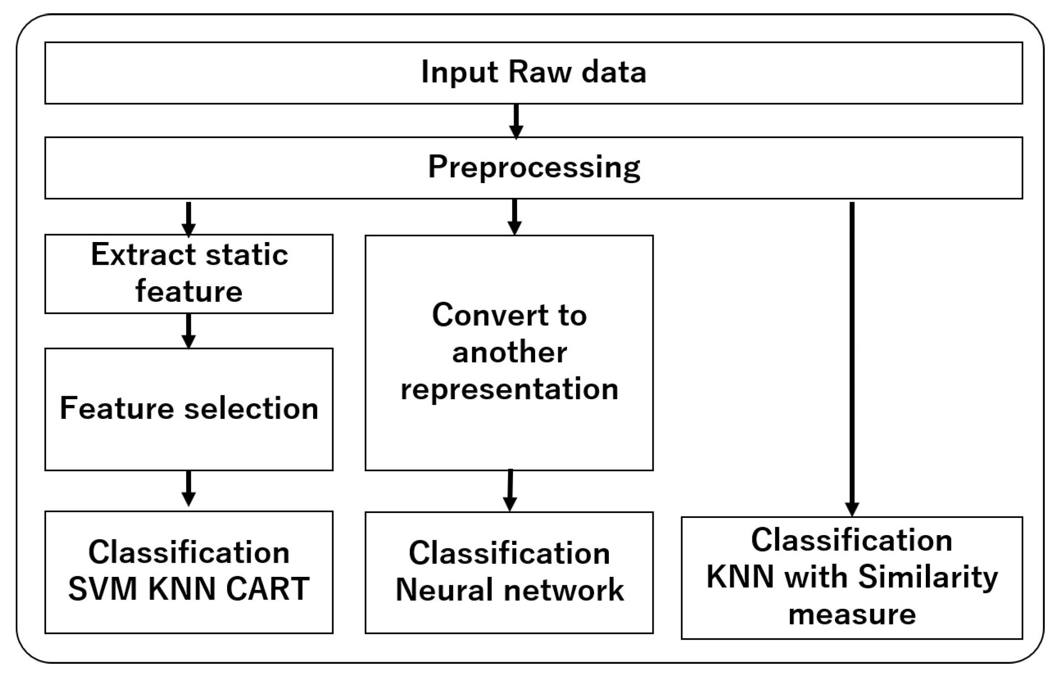
Approaches for time series classification can also roughly be grouped into approaches based on raw time series data and approaches based on transformed data in which the time series is converted as a set of feature vectors. Figure 1 represents the grouping of popular time series classification approaches after preprocessing of the data. The group of approaches on the left consists of representation of time series as a vector of global static features, selection of the most appropriate features and classification done by traditional machine learning models such as SVM (support vector machine), KNN (k-nearest neighbour) or CART (decision tree). The block on the right represents the approaches for classification with raw time series by KNN using various similarity measures. The middle group represents various representation schemes (feature extraction) for classification by deep neural networks or other machine learning classifiers. In this work our approach falls into this category.
2.1. Feature-Based Representation
Feature-based approches for classification is generally faster than raw time series-based approaches. Feature extraction from time series can be done either in time domain or in frequency domain. Moreover features can also be derived from subsequences of a time series characterizing local patterns or from the whole time series capable of expressing the global patterns. Features computed from different subsections of a time series are combined to form a bag of feature framework TSBF for classification of time series in Baydogan et al. [28].
Some of the feature-based representations of time series convert time series into a vector of feature values which are generally average statistical measures of time series over a window (whole time series is divided into a sequence of fixed length or sliding windows) of ordered sequences like mean, standard deviation, skewness, kurtosis and their successive increments [29]. Those features are unable to preserve the dynamic information embedded in the time series. Another class of feature-based representation consists of various transformations of time series in frequency domain such as DFT (Discrete Fourier Transformation), SVD (Singular Value Decomposition), DCT (Direct Cosine Transformation), DWT (Discrete Wavelet Transformation) and so forth. Timmet et al. [30] used a variety of time and frequency domain features to represent hand tremor time series. Morchen [31] used different features from the frequency domain for classification of different time series. Wang [32] used 13 features for classification of univariate and multivariate time series.
In feature-based approaches for TSC, classification accuracy is highly dependent on the extracted and selected features rather than the classification model. The choice of features to characterize a time series is subjective and non systematic. The best feature subset is also task dependent and there is no one particular way of choosing features for all time series classification problems. All the approaches need to take care of preprocessing data and selecting appropriate features for efficient classification.
2.2. Time Series Classification with Deep Neural Network
Deep neural networks (DNN), known to be capable of automatic feature extraction, are now becoming very popular and have many successful applications in the field of image processing [33]. In addition to images, sequential text and audio data can also be processed successfully with deep neural networks. Motivated by their success, recently DNN, especially convolutional neural networks (CNN), are increasingly used in TSC problems as time series resembles text data and audio in terms of their sequential nature.
A multi channel CNN (MC-CNN) in which filters are applied to each channel and the features are flattened across channels to input to a fully connected layer is proposed in Zheng et al. [34]. A multiscale convolutional neural network (MCNN) has been proposed for univariate time series classification in which three types of representation (down sampling, skip sampling and sliding window) for preprocessing of raw time series are used to input to the network [35]. Another research work is based on the similar idea of exploiting simultaneously multiple branches of the same type of representation for time series classification [36].
Wang [22] suggested two other CNNs for time series classification, the fully convolutional neural network (FCN) without subsampling layers and ResNet (Residual Network). With the addition of some learning techniques, these two models produce better performance than MCNN or COTE, as is demonstrated by simulation with UCR benchmark data sets. An ensemble method of deep networks is proposed in Reference [37] in which LSTM (Long Short Term Memory) and FCN models are individually used and their outputs are concatenated and passed though a softmax classifier for final decision. Although deep neural networks achieve quite good classification accuracy for time series classification problems, high preprocessing effort and tuning of large set of hyperparameters make them difficult to use in a real situation.
2.3. Recurrence Plot for Deep Neural Network
There are basically two main approaches for time series classification with convolutional neural networks. In one approach, traditional CNN is modified to accept 1-dimensional time series as input and in the other approach, time series is converted into a 2D image to be used with conventional CNN. There are various methods for transforming time series signals into images using specific imaging methods like Gramian Angular Fields (GAF) [24,25], Markov Transtion Field (MTF) [26] and Recurrence Plot (RP), a tool in chaos theory to visualize time series.
Silva et al. [38] used the Campana- Keogh distance measure to estimate image similarity as a similarity measure (CK-1) between two recurrence plots corresponding to two time series and found an improvement of classification accuracy compared to Euclidean distance and dynamic time warping. Hatami et al. in Reference [39] used RP as an input to CNN for TSC problems. In a subsequent paper [40], the authors used bag of feature concepts on recurrence plot and generated bag of recurrence patterns for representation of time series for classification with Support Vector Machine (SVM) classifier. Michael et al. [41] defined a cross recurrence plot (CRP) as an extension of recurrence plot to visualize similar recurring patterns in two time series and proposed another similarity measure called the cross recurrence plot compression distance (CRPCD), which is a modification of the work in Reference [38]. Recurrence quantification analysis (RQA) [42] was developed to quantify differences in recurrence plots of two dynamical systems. It is used as a similarity measure in time series classification tasks in several recent works [43,44,45]. It seems that there is no research considering the modification of recurrence plot to be used with deep networks for better classification accuracy in a time series classification problem.
Recurrence plot (RP) created by Eckman [27], is a tool to visualize recurrent behaviour such as periodicity or irregular cyclicity, a typical phenomenon in nonlinear dynamical systems that generates the time series. It is a 2D plot for encoding 1D time series which provides a way to visualize the recurrence behaviour of trajectory through a phase space and enables us to investigate certain aspects of the m-dimensional phase space trajectory through a 2D representation. It can be defined by the following equation:
where x is a time series of length n, and are the subsequences observed at i and j positions of the time series, is a norm (e.g., Euclidean norm) between the observations, is the recurrence threshold. It is chosen in such a way that the noises are filtered out but the recurrence structures are preserved. is the Heaviside function. According to Equation (1), the recurrence of phase state at time i and j are placed in the square matrix with black and white dots. Recurrence is marked by the black dots.
Cross recurrence plot (CRP) is an extension of RP which shows all the times when a state in one time series occurs in the other time series. When the length of the two time series n and l respectively differs, the CRP matrix becomes non-square.
3. Proposed TSC Approach by DNN with Modified Recurrence Plot
In this work, time series classification with deep neural network with a proposed modification of recurrence plot for improvement of classification performance has been investigated. Based on our literature survey we considered two architectures, fully convolutional networks (FCN) and Residual Network (ResNet) with three types of data representation, the first one being traditional recurrence plot and the two others being proposed modifications for time series classification.
The first step in the proposed classification approach is the recurrence plot generation. It is a simple tool for reconstruction of nonlinear dynamical system from the observed time series based on the concept of the embedding theorem. The embedding theorem proposed by Taken and expanded by Sauer [46] guarantees that the phase space of time delayed vectors with sufficiently large dimension will capture the structure of the original phase space.
A deterministic time series signal can be embedded as a sequence of time delay co-ordinate vector known as experimental attractor, with an appropriate choice of embedding dimension m which is the minimum number of co-ordinates needed to represent the time series with no overlapping in the state space and delay time which is the time lag of the time series points taken as coordinates.
Now for correct reconstruction of the attractor, a fine estimation of embedding parameters (m and ) is needed. There are a variety of heuristic techniques for estimating those parameters [47]. The most popular method of estimating m is False Nearest Neighbour proposed by Kennel and the most popular technique for estimating is Average Mutual Information.
3.1. Recurrence Plot (RP) Generation
After estimation of the embedding parameters, a time series can be converted to recurrence plot. The recurrence plot is an array of dots in a square, where a dot is placed at (i, j), whenever is sufficiently close to . By choosing an embedding dimension m, the m-dimensional orbit of can be constructed by the method of time delay. Then is chosen such that the ball of radius centred at in contains a reasonable number of other points of the orbit. Finally, a dot at each point (i, j) for which is in the ball of radius centred at , is plotted and the generated image is called the recurrence plot. The practical steps of generation are:
- Estimation of proper embedding parameters m and .
- Embedding of time series data with Equation (3).
- Calculation of Euclid distance to generate .
- The square distance matrix is finally converted to grey scale image as the input to CNN for classification.
Now the square matrix generated is symmetric across the diagonal, lower left triangular part and upper right triangular part contains the same information.
3.2. Proposed Modified Recurrence Plot (Recurrence Plot Raw RP1)
In our previous study [48] for time series classification on 85 benchmark data sets from UCR repository using CNN (convolutional Neural Network) similar to the CNN used in Reference [39], it has been found that the two dimensional recurrence plot representation of input data with CNN produces better classification accuracy compared to the classification accuracy of one dimensional raw time series data with 1NN classifier and Euclid distance or DTW as the similarity measures for most of the data sets. The simulation study was done with recurrence plot generation for different m and values, However the following issues were noticed that need further consideration.
- It was found that for some data sets it was possible to improve classification accuracy by tuning the parameters m and while in other data sets, tuning did not work. As an explanation for this, it is assumed that, during generation of the recurrence plot, if the change in the time series is small, the distance values in the matrix become close to zero, resulting in poor classification accuracy while those types of time series are better classified with the 1NN classifier and DTW measure using the raw time series.
- Due to the symmetric nature of the square recurrence plot transformed image across the diagonal, only one triangular part is needed for representation of the data, the other part is redundant, which has an effect on increasing computational burden.
- The computational cost increases with the size of the input image, so recurrence plot image size should be the smallest needed to preserve the characteristic pattern of the time series for classification, so resizing of the input image is needed to reduce computational burden.
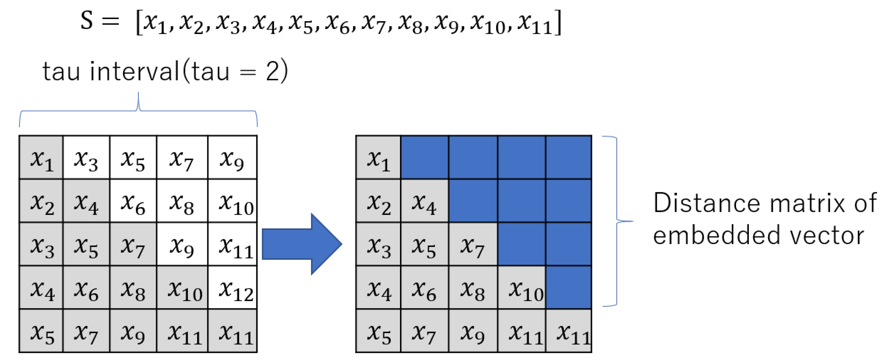
To alleviate the above points, a modified image representation of the input data is proposed here where one triangular half of the square image retains the recurrence plot of the input data and the other part contains information from the raw data to remove the redundancy in the input image representation and to take care of different types of time series to be classified with similar accuracy. Finally the image is resized and checked that it does not affect classification accuracy. The steps of generation of the transformed image are summarized below and is shown in Figure 2.
- Estimation of proper embedding parameters m and .
- Embedding of time series data with Equation (3).
- Calculation of Euclid distance to generate the distance matrix .
- Normalization of the distance values to lie between 0.0 and 1.0 to form the square matrix A.
- Another square matrix B is formed with the original time series values sifted by . Let us suppose that the normalized original time series is represented by S consisting of 11 points. Its distribution in a square matrix B with is shown in the left square of the figure.
- The final square matrix F is designed by combining A and recurrence plot information from B in which upper triangle represents the upper triangle (except the diagonal) of the recurrence plot values and the lower triangle represents the lower triangle (with the diagonal) of the original square matrix A as shown in the right square of the figure.
- Finally, square matrix F is converted to image (RP1) and optimized to proper size as a representation of the time series.
Recurrence Plot DTW (RP2)
In another version of time series representation, step 3 of the recurrence plot algorithm for distance matrix calculation is modified and dynamic time warping (DTW) is used. The DTW distance matrix by DTW (the distance between the time series and with the best alignment) is obtained by the following Alogrithm 1.
| Algorithm 1: Calculation of DTW |
| for to n do for to l do end for end for return |
represents the euclid distance between and .
3.3. Classification by FCN and ResNet
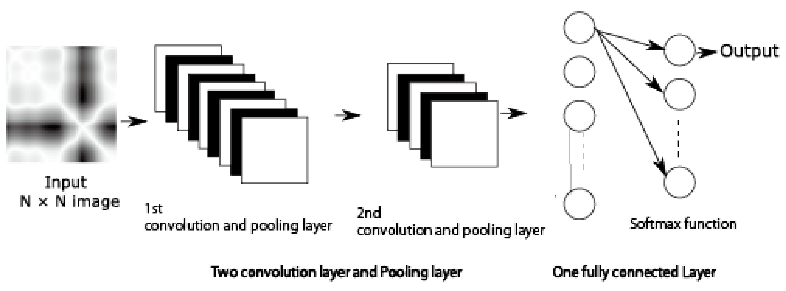
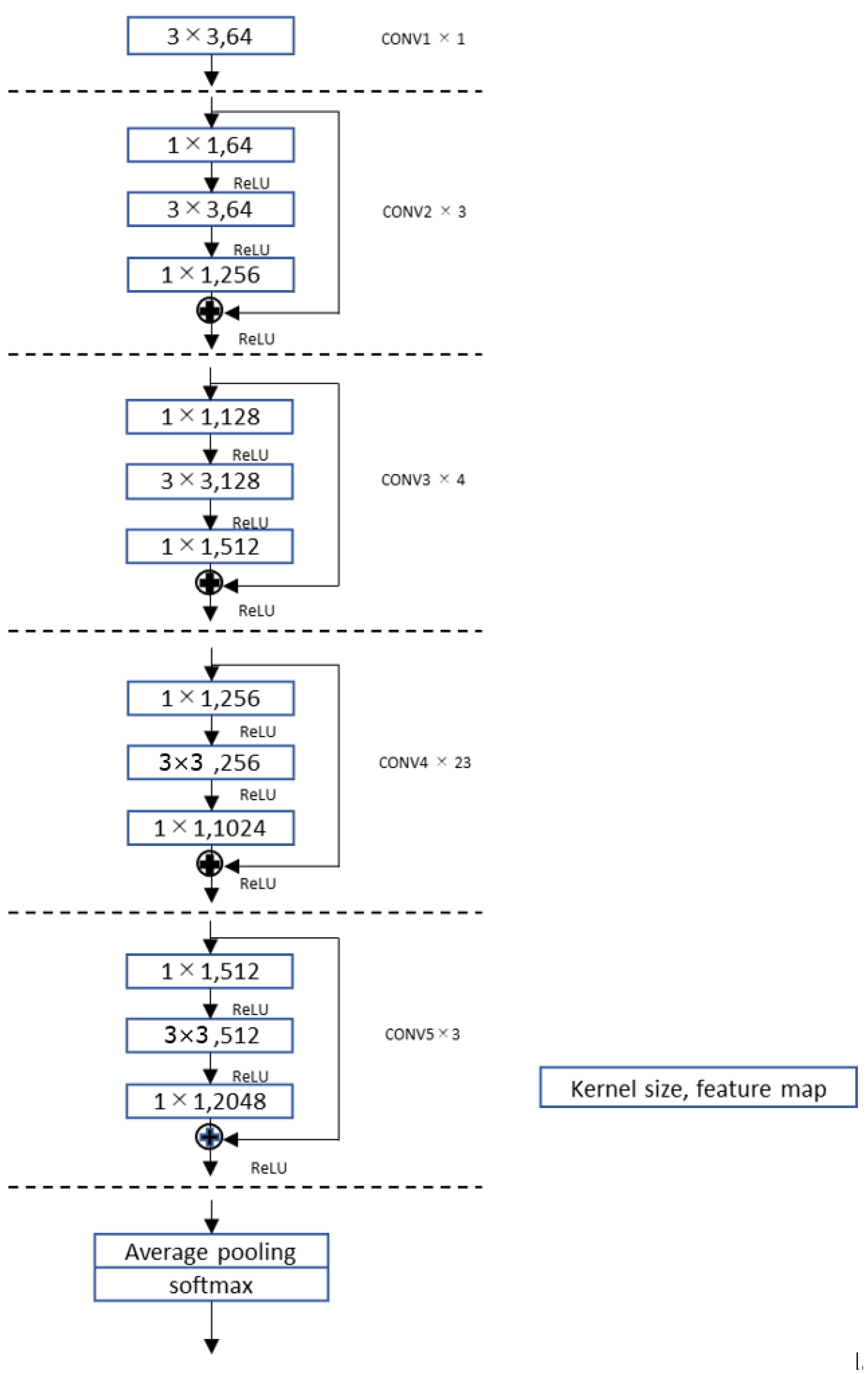
In this work, fully convolutional neural network (FCN) and Residual network (ResNet) has been used for time series classification. The basic structure of the FCN used is shown in Figure 3. It consists of the input layer followed by two sets of convolutional layer and max-pooling layer, two fully connected layers and output layer. The number of neurons in the first fully connected layer depends on the input image size (input image size × feature map size) and in the second fully connected layer is 512. We used three sizes of input images , , . The detailed parameters used after some trial and error with the model are shown in Table 1. The basic structure of the ResNet used in this work is same as used in Reference [49] and is shown in Figure 4. The input image size for ResNet is restricted to for all time series.
4. Comparative Study and Simulation Experiments
The proposed approaches based on FCN and ResNet with three types of recurrence plot-based data representation RP, RP1 and RP2 for time series classification have been evaluated with benchmark data sets from UCR archive. A comparative study has been done to verify the classification efficiency of the proposed approaches in comparison with some other popular and successful approaches for TSC. Here we selected the following classification approaches for comparative study.
- 1NN classifier with Euclid distance as the similarity measure using raw time series. This is the simplest approach and has the lowest computational cost. However, this approach cannot be used to compare two time series of unequal length.
- 1NN classifier with DTW (dynamic time warping) as the similarity measure between two time series. This is the most popular approach; it produces high classification accuracy but has high computational cost. The algorithm is presented in the previous section.
- 1NN classifier with longest common subsequence (LCSS) [50] as the similarity measure. LCSS is a variant of edit distance which also matches two time series by allowing them to stretch like DTW. It has two parameters ND a matching threshold. Two points from two time series are considered to match if their distance is less than and , the warping threshold which controls the window size for matching. It is known to be more robust to noise and outliers compared to DTW.
- CrossTranslation error (CTE), similarity measure for two time series, was developed by one of the authors previously for the online signature verification problem, which is based on the delay vector representation of time series. The details can be found in Reference [51]. It is computationally very light, although classification accuracy is poor. The calculation process is described in short here.
- Let and denote m-dimensional delay vectors generated from time series and time series respectively according to Equation (3).
- A random vector is picked up from . Let the nearest vector of from be . The index for the nearest vector is defined as follows;
- For the vectors and , the transition in each orbit after one step is calculated as follows;
- Cross Translation Error (CTE) is calculated from and aswhere denotes average vector between and .
- is calculated for L times for a different selection of random vector and the median of () is calculated asThe final cross translation error is calculated by taking the average, repeating the procedure Q times to suppress the statistical error generated by random sampling in the step (3).
- Time series bag of features (TSBF) is an an extension of Time series forest (TSF) with multiple stages. The first stage generates a subseries classification problem and the second stage forms class probability estimates for each subseries. The third stage constructs a bag of features from these probabilities and finally a random forest classifier is built on the bag of feature representation. The details can be found in Reference [28].
- We also used one dimensional FCN ( Convolutional Neural Network) and ResNet and used raw time series data for classification to compare the effect of 2D recurrence plot approach for time series classification compared to 1D raw time series data. Due to limitation of computational resources while implementing ResNet, we compressed the time series for recurrence map generation, we used the same compressed time series for one dimensional version of FCN and ResNet for fair comparison.
4.1. Dataset Used
The simulation experiments were done with the benchmark datasets from UCR/UEA time series classification archive [52]. We used 85 data sets, details of which are presented on the archive website. The data sets contain time series of various characteristics, length ranges from 24 to 2709, number of classes varies from 2 to 60. Some data sets have a very small training set size. The data sets are collected from different application domains and can be divided into seven categories as Image Outline (29), Sensor Readings (16), Motion Capture (14), Spectrographs (7), ECG measurements (7) Electric device profiles (6) and Simulated Data (6), the numbers in bracket represents the numbers of data sets in the said category.
4.2. Simulation Experiments
Following simulation experiments for time series classification with benchmark data sets, training and test sets were used, as is mentioned in the original data set with 10 fold cross validation for each classifier. For convolutional neural network CNN, some trial and error experiments were done for appropriate hyper parameter setting and the hyper parameters are set for the best results and are represented in the next section. For ResNet, due to time limitations, we used previously reported parameters.
- FCN classifier with three types of recurrence plot representation (RP, the original one, RP2, in which DTW is used for distance calculation for recurrence plot, RP1, our proposed modified recurrence plot in which raw data is also combined with the recurrence plot)
- The above experiments are repeated with ResNet with the same three types of recurrence plots.
- Experiments were done with Nearest Neighbor classifier with Euclid and DTW using the original raw time series.
- 1NN classifier with edit distance-based approaches, LCSS (longest common subsequence), TWED (time warped edit distance) and MSM (Move-Split-Merge), are used for classification using the original raw time series.
- Cross transtational error (CTE) based on the concept of multidimensional delay vector representation with 1NN classifier.
- A feature-based approach TSBF with random forest classifier is used.
We attempted to implement ensemble-based algorithms on the data sets but due to lack of proper computing resources, we restricted our comparative study to non-ensemble algorithms.
5. Simulation Results and Analysis
Table 2 represents classification accuracies of 85 data sets with different classification approaches. In all tables, in every row, the highest value is presented in bold which represents the best classification accuracy obtained for the particular data set. Column 1 represents data sets, column 2 represents classification accuracies by FCN with traditional recurrence plot similar in the work presented in Reference [39]. Columns 3, 4 and 5 represent classification accuracy values for FCN with recurrence plot RP2, FCN with proposed modified recurrence plot RP1 and ResNet with RP1 respectively. We found that RP1 produces better classification accuracies than RP and RP2, so we did not present (RP2 + ResNet) results. The rest of the columns represent classification accuracies for Euclid, DTW, LCSS, CTE and TSBF. We did not include the results of TWED and MSM as those have poor classification accuracies compared to the methods presented in the table. It is found that no algorithm is best for all the data sets. Though TSBF produces the best classification accuracy for most of the data sets, average classification accuracy over 85 data sets is not the highest among all the methods. Our proposed method (RP1 + ResNet) achieves the highest average classification accuracy over 85 data sets. RP2 uses DTW for distance calculation, which increased computational cost as well as accuracy for some of the data sets, as a whole the increase in classification accuracy is not so significant compared to the increase in computational cost. However, our proposed modification of recurrence plot RP1 seems to have the best effect on the increase of classification accuracy. This modification does not increase the computational cost. From this table it can be assumed that TSBF, RP1+FCN and RP1 + ResNet are the effective classifiers.
Table 3 represents the comparison of classification accuracies of different one dimensional deep networks with raw time series input and two dimensional deep network-based algorithms with recurrence plot input. We excluded TSBF here to focus on the results of recurrence plot-based methods. Column 4 and column 6 represent the results of 1D convolutional neural network and 1D ResNet, respectively. It is found that the results of two dimensional deep networks with recurrence plot input are far better than one dimensional deep networks with raw time series input for most of the data sets. From this table it is also found that the classification accuracy of column 7 (RP1 + ResNet) is the highest for the most of the data sets. It can be concluded that ResNet with our proposed modified recurrence plot input produces the best average classification accuracy and the highest classification accuracy for most of the data sets. Also, the variability of the classification accuracies among different data sets is the lowest (same as DTW).
Table 4 represents the comparison of the classification performance of the our proposed classification algorithm, ResNet with modified recurrence plot RP1 as input (RP1 + ResNet), the best among all recurrence plot-based algorithms and TSBF, the best classifier among all others (where recurrence plot is not used) considered in this work. It is clearly seen that our proposed method is better in classification performance for greater number of data sets compared to TSBF.
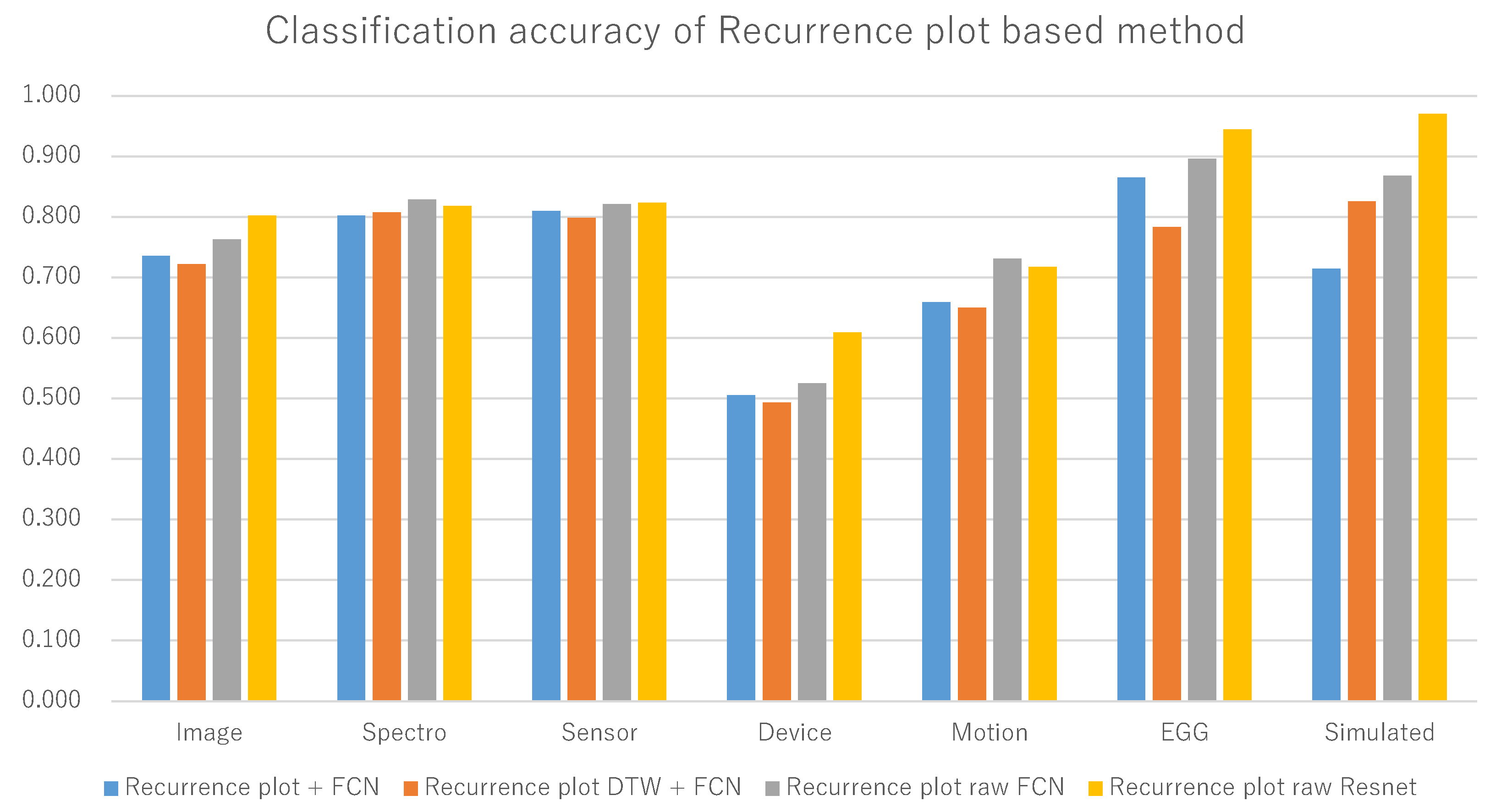
Table 5 displays the average classification accuracies for each category of time series with all the algorithms. It is clear from Table 5 that ResNet with our proposed modified recurrence plot RP1 is the best algorithm for four categories of time series data among seven categories, one category (Spectro) has the highest classification accuracy with (RP1 +FCN). If we choose only the algorithm (RP1+ResNet) for comparison, it will produce highest classification accuracy for five categories among a total of seven categories because, for the Spectro category, this algorithm has the second best value. Only for two categories, Device and Motion, did TSBF outperform our proposed method. It is also found that ResNet with RP1 has the best performance among all other recurrence plot-based methods (as noted in the average classification accuracy of 85 data sets in the table). This is also evident in Figure 5, in which recurrence plot-based methods are compared where recurrence plot denotes RP, recurrence plot with DTW represents RP2 and recurrence plot raw represents RP1. It is seen from Figure 5, that (RP1 + ResNet) has the best classification accuracy for 5 categories and is not so significantly different from (RP1 + FCN) in the other two categories.
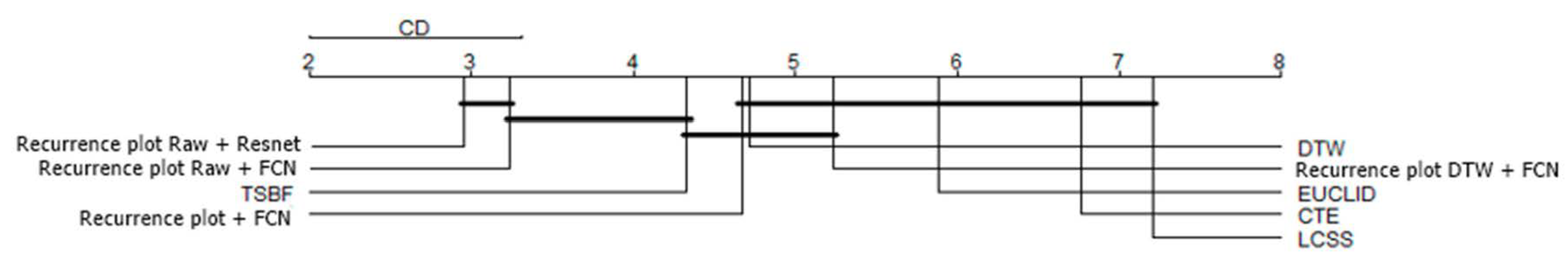
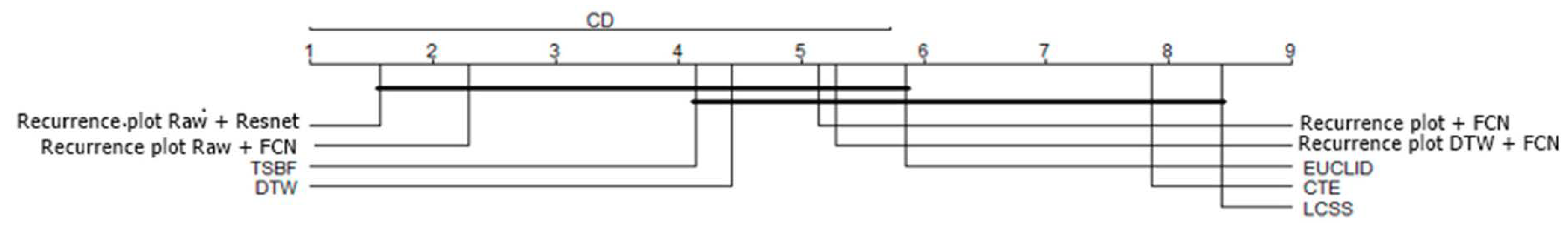
For testing the statistical significance between different approaches, we followed the methodology described in Reference [53]. Critical difference (CD) plots of different algorithms for individual 85 data sets and categorized into 7 group of data sets respectively are presented in Figure 6 and Figure 7 respectively in which recurrence plot denotes RP, recurrence plot with DTW represents RP2 and recurrence plot raw represents RP1. In both the figures, it is seen that our proposed approach (RP1 + ResNet) ranks higher than other approaches. From Figure 6, it is seen that the algorithm (RP1 + ResNet) has the highest rank and there is no significant difference between the algorithms (RP1 + ResNet) and (RP1 + FCN), which are significantly better than other algorithms. From Figure 7 the same conclusion can be drawn.
For consideration of computational cost, it is difficult to compare all the algorithms by implementing all of them in the same platform. It is needless to say that the parameter search of deep neural network architectures takes time and our reported results might not constitute the most optimized architecture. On the other hand, for NN-DTW, warping window size has a considerable effect on the final accuracy and we did not put significant effort into searching for the best warping window. As a rough comparison, our proposed representation technique based on recurrence plot and deep network considerably improved classification accuracy without incurring additional computational cost compared to other popular non ensemble and deep network-based algorithms.
6. Conclusions
In this paper, the effect of time series data representation methods for time series classification problems in terms of increased classification accuracy with affordable computational cost and intrepretability has been studied. Our study focussed mainly on recurrence plot-based representation of time series for use with deep network-based classifiers. Because there are several deep network architectures and, from the reported results, it is found that CNN and ResNet perform better than others in time series classification problems, fully convolutional network (FCN) and residual network (ResNet) have been used in our work. A new modified recurrence plot representation of time series data set has been proposed which judiciously includes information from raw time series in the recurrence plot framework without much additional computational cost for improvement of classification accuracy.
The use of recurrence plot as the input representation form increases the interpretability of the classification method compared to the raw time series input. Deep networks are known to be black boxes which inherently extract the features of the time series for grouping. Although it is convenient, this process is invisible to users. Recurrence plots are more visually interpretable than raw time series. Humans can deploy the results of classification by deep network later to establish a correlation between the structure of the recurrence plot with the categories of time series. Interpretability of classification process can also be increased by extracting explicit features from the time series and then classifying the time series by those features which will allow users to relate the classes with the characteristics of the time series. However, the proper selection of a feature set is important for efficient classification and there is no general way to do that.
In our work, the modification of recurrence plot by mixing of information from raw time series data with the recurrence plot allows us to consider static and dynamic features of the time series simultaneously and extends the use of recurrence plot to a wide variety of time series data. Due to computational resource limitations, we optimized the size of recurrence plot in such a way that the computational limitations could be overcome without much degradation of classification accuracy and we selected 50 × 50 image size for input to ResNet for all time series irrespective of their original length according to our computational environment. The computational cost of deep network based approaches with original time series input increases with the increase of the length of time series as the network complexity (number of parameters) increases which in turn increases the training time. Our approach is an attempt to optimize computational burden, classification accuracy with general applicability to different types of time series and also to add interpretability. Of course increasing the size of recurrence plot might increase the classification accuracy for some time series. We did not tuned the size for all the time series individually at this stage. There is a scope of further improvement of classification accuracy at the cost of more computation time.
A comparative study has been done with some of the state-of-the art algorithms and it was found that our proposed approach can produce better classification accuracy for most of the data sets. For comparison, we did not include ensemble algorithms. Although ensemble algorithms produce better classification accuracy, their computational cost is too high to find out the proper combination. It has been found from the comparative study that our proposed algorithm performs better than popular traditional non-ensemble algorithms for time series datasets for most of the domains available from the benchmark data set repository.
Author Contributions
Conceptualization, B.C.; Investigation, K.N.; Methodology, K.N.; Software, K.N.; Writing—original draft, K.N.; Writing—review & editing, B.C.
Funding
This research received no external funding.
Acknowledgments
This research was supported by PRML laboratory of Department of Software and Information Science, Iwate Prefectural University, Japan.
Conflicts of Interest
The authors declare no conflicts of interest.
References
- Esling, P.; Agon, C. Time series data mining. ACM Comput. Surv. 2012, 45, 12.1–12.34. [Google Scholar] [CrossRef] [Green Version]
- Tamilarasi, K.; Nithya Kalyani, S. A survey on signature verification based algorithms. In Proceedings of the IEEE International Conference on Electrical, Instrumentation and Communication Engineering (ICEICE), Karur, India, 27–28 April 2017; pp. 1–3. [Google Scholar]
- Wang, J.; Liu, P.; She, M.F.H.; Nahavandi, S.; Kouzani, A. Bag-of-words representation for biomedical time series classification. Biomed. Signal Process. Control 2013, 8, 634–644. [Google Scholar] [CrossRef] [Green Version]
- Fisher, T.; Krauss, C. Deep Learning with Long Short-Term Memory Networks for Financial Market Predictions. Eur. J. Oper. Res. 2018, 270, 654–669. [Google Scholar] [CrossRef] [Green Version]
- Lara, O.D.; Labrador, M. A survey on human activity recognition using wearable sensors. IEEE Commun. Surv. Tutor. 2013, 15, 1192–1209. [Google Scholar] [CrossRef]
- Singh, D.; Merdivan, E.; Psychoula, I.; Kropf, J.; Hanke, S.; Geist, M.; Holzinger, A. Human activity recognition using recurrent neural networks. In Machine Learning and Knowledge Extraction; lecture notes in computer science lncs 10410; Springer/Nature: London, UK, 2017; pp. 267–274. [Google Scholar] [CrossRef] [Green Version]
- Kini, B.V.; Sekhar, C.C. Large margin mixture of AR models for time series classification. Appl. Soft Comput. 2013, 13, 361–371. [Google Scholar] [CrossRef]
- Antonucci, A.; De Rosa, R.; Giusti, A.; Giusti, A.; Cuzzolin, F. Robust classification of multivariate time series by imprecise hidden Markov models. Int. J. Approx. Reason. 2015, 56, 249–263. [Google Scholar] [CrossRef]
- Kim, S.B.; Han, K.S.; Rim, H.C.; Myaeng, S.H. Some effective techniques for naive bayes text classification. IEEE Trans. Knowl. Data Eng. 2006, 18, 1457–1466. [Google Scholar]
- Lal, T.N.; Schroder, M.; Hinterberger, T.; Weston, J.; Bogdan, M.; Birbaumer, N.; Scholkopf, B. Support Vector Channel Selection in BCI. IEEE Trans. Biomed. Eng. 2004, 51, 1003–1010. [Google Scholar] [CrossRef] [Green Version]
- Chakraborty, B. Feature selection and classification techniques for multivariate time series. In Proceedings of the Second International Conference on Innovative Computing, Information and Control (ICICIC 2007), Kumamoto, Japan, 5–7 September 2007. [Google Scholar]
- Ye, L.; Keogh, E. Time series shapelets: A new primitive for data mining. In Proceedings of the ACM SIGKDD International Conference of Knowledge Discovery and Data Mining, Paris, France, 28 June 28–1 July 2009; pp. 947–956. [Google Scholar]
- Yoon, H.; Yang, K.; Sahabi, C. Feature subset selection and feature ranking for multivariate time series. IEEE Trans. Knowl. Data Eng. 2005, 17, 1186–1198. [Google Scholar] [CrossRef] [Green Version]
- Berndt, D.J.; Clifford, J. Using dynamic time warping to find patterns in time series. In Proceedings of the 3rd International Conference on Knowledge Discovery and Data Mining (AAAIWS 94), Seattle, WA, USA, 31 July–1 August 1994; pp. 359–370. [Google Scholar]
- Wang, X.; Mueen, A.; Ding, H.; Trajcevski, G.; Scheuermann, P.; Keogh, E. Experimental comparison of representation methods and distance measures for time series data. Data Min. Knowl. Discov. 2013, 26, 275–309. [Google Scholar] [CrossRef] [Green Version]
- Lines, J.; Bagnall, A. Time series classification with ensembles of elastic distance measures. Data Min. Knowl. Discov. 2015, 29, 565–592. [Google Scholar] [CrossRef]
- Bagnall, A.; Lines, J.; Hills, J.; Bostrom, A. Time series classification with COTE: The collective of transform-based ensembles. IEEE Trans. Knowl. Data Eng. 2015, 27, 2522–2535. [Google Scholar] [CrossRef]
- Lines, J.; Taylor, S.; Bagnall, A. Time series classification with HIVE-COTE: The hierarchical vote collective of transformation based ensembles. ACM Trans. Knowl. Discov. Data 2018, 12, 52:1–52:35. [Google Scholar] [CrossRef] [Green Version]
- Bagnall, A.; Bostrom, A.; Large, J.; Lines, J. The great time series classification bake off: A review and experimental evaluation of recent algorithmic advances. Data Min. Knowl. Discov. 2017, 31, 606–660. [Google Scholar] [CrossRef] [Green Version]
- Fawaz, H.I.; Forestier, G.; Weber, J.; Idoumghar, L.; Muller, P.A. Deep Learning for time series classification: A review. Data Min. Knowl. Discov. 2019, 33, 917–963. [Google Scholar] [CrossRef] [Green Version]
- Sadouk, L. CNN Approaches for Time Series Classification. Convolutional Neural Netw. 2018. [Google Scholar] [CrossRef] [Green Version]
- Wang, Z.; Yan, W.; Oates, T. Time series classification from scratch with deep neural networks: A strong base line. In Proceedings of the IEEE IJCNN, Anchorage, AK, USA, 14–19 May 2017; pp. 1578–1585. [Google Scholar]
- Borovkova, S.; Tsiamas, S. An ensemble of LSTM neural networks for high-frequency stock market classification. J. Forecast. 2019, 38, 600–619. [Google Scholar] [CrossRef] [Green Version]
- Wang, Z.; Oates, T. Imaging time series to improve classification and imputation. In Proceedings of the International Joint Conference on Artificial Intelligence (IJCAI), Buenos Aires, Argentina, 25–31 July 2015; pp. 3939–3945. [Google Scholar]
- Wang, Z.; Oates, T. Encoding time series as images for visual inspection and classification using tiled convolutional neural networks. In Proceedings of the AAAI Conference, Austin, TX, USA, 25–30 January 2015; pp. 40–46. [Google Scholar]
- Wang, Z.; Oates, T. Spatially encoding temporal correlations to classify temporal data using convolutional neural networks. arXiv 2015, arXiv:1509.07481v1. [Google Scholar]
- Eckmann, J.; Kamphorst, S.; Ruelle, D. Recurrence plots of dynamical systems. EPL (EuroPhys. Lett.) 1987, 4, 973–977. [Google Scholar] [CrossRef] [Green Version]
- Baydogan, M.G.; Runger, G.; Tuv, E. A Bag-of-Features Framework to classify Time Series. IEEE Trans. Pattern Anal. Mach. Intell. 2013, 35, 2796–2802. [Google Scholar] [CrossRef]
- Nanopoulos, A.; Alcock, R.; Manolopoulos, Y. Feature- based classification of time-series data. In Information Processing and Technology; Nova Science Publishers, Inc.: New York, NY, USA, 2001; pp. 49–61. [Google Scholar]
- Timmer, J.; Gantert, C.; Deuschl, G.; Honerkamp, J. Characteristics of hand tremor time series. Biol. Cybern. 1993, 70, 75–80. [Google Scholar] [CrossRef] [PubMed]
- Morchen, F. Time Series Feature Extraction for Data Mining Using DWT and DFT; Technical report; Phillips University Marburg: Marburg, Germany, 2003. [Google Scholar]
- Wang, X.; Smith, K.; Hyndman, R. Characteristic based clustering for time series. Data Min. Knowl. Discov. 2006, 13, 335–364. [Google Scholar] [CrossRef]
- LeCun, Y.; Bengio, Y.; Hinton, G. Deep Learning. Nature 2015, 521, 436–444. [Google Scholar] [CrossRef] [PubMed]
- Zheng, Y.; Liu, Q.; Chen, E.; Ge, Y.; Zhao, J.L. Exploiting multichannels deep convolutional neural networks for multivariate time series classification. Front. Comput. Sci. 2016, 10, 96–112. [Google Scholar] [CrossRef]
- Cui, Z.; Chen, W.; Chen, Y. Multi-scale convolutional neural network for time series classification. arXiv 2016, arXiv:1603.06995. [Google Scholar]
- Wang, W.; Chen, C.; Wang, W.; Rai, P.; Carin, L. Earliness- aware deep convolutional networks for early time series classification. arXiv 2016, arXiv:1611.04578. [Google Scholar]
- Karim, F.; Majumdar, S.; Darabi, H.; Chen, S. LSTM Fully Convolutional Networks for Time Series Classification. IEEE Access 2018, 6, 1662–1669. [Google Scholar] [CrossRef]
- Silva, D.F.; Batista, G.E. Time Series Classification Using Compression Distance of Recurrence Plots. In Proceedings of the IEEE 13th International Conference on Data Mining, Dallas, TX, USA, 7–10 December 2013; pp. 687–696. [Google Scholar]
- Hatami, N.; Gavet, Y.; Debayale, J. Classification of time series images using deep convolutional neural networks. In Proceedings of the International conference on machine vision (ICMV), Vienna, Austria, 13–15 November 2017. [Google Scholar]
- Hatami, N.; Gavet, Y.; Debayale, J. Bag of recurrence patterns representations for time series classification. Pattern Anal. Appl. 2018, 22, 877–887. [Google Scholar] [CrossRef] [Green Version]
- Michael, T.; Spiegel, S.; Albayrak, S. Time Series Classification using Compressed Recurrence Plots. In Proceedings of the NFMCP Workshop @ ECML-PKDD 2015, Porto, Portugal, 7 September 2015; pp. 178–187. [Google Scholar]
- Spiegel, S.; Marwan, N. Time and Again: Time Series Mining via Recurrence Quantification Analysis. In Proceedings of the ECML PKDD, Rive del Garda, Italy, 19–23 September 2016. [Google Scholar]
- Spiegel, S.; Jain, B.J.; Albayrak, S. A Recurrence Plot-Based Distance Measures. In Translational Recurrences. Springer Proceedings in Mathematics & Statistics; Marwan, N., Riley, M., Giuliani, A., Webber, C., Jr., Eds.; Springer: Cham, Switzerland, 2014; Volume 103. [Google Scholar]
- Spiegel, S.; Albayrak, S. An order-invariant time series distance measure-Position on recent developments in time series analysis. In Proceedings of the International Joint Conference on Knowledge Discovery, Knowledge Engineering and Knowledge Management (KDIR), Barcelona, Spain, 4–7 October 2012. [Google Scholar]
- Spiegel, S. Discovery of driving behavior patterns. In Smart Information Services; Computational Intelligence for Real-Life Applications; Springer: Berlin/Heidelberg, Germany, 2015. [Google Scholar]
- Alligood, K.T.; Sauer, T.; Yorke, J. Chaos: An Introduction to Dynamical Systems; Springer: New York, NY, USA, 1997. [Google Scholar]
- Aberbanel, H.D.I. Analysis of Observed Chaotic Data; Springer: New York, NY, USA, 1996. [Google Scholar]
- Nakano, K.; Chakraborty, B. Effect of Data Represntation Method for Effective Mining of Time Series Data. In Proceedings of the 2019 IEEE International Conference on Big Data and Smart Computing (BigComp), Kyoto, Japan, 27 February 27–2 March 2019; pp. 1–6. [Google Scholar]
- He, K.; Zhang, X.; Ren, S.; Sun, J. Deep residual learning for image recognition. In Proceedings of the IEEE Conference of Computer Vision and Pattern Recognition (CVPR), Las Vegas, NV, USA, 27–30 June 2016; pp. 770–778. [Google Scholar]
- Vlachos, M.; Gunopoulos, D.; Kollios, G. Discovering Similar Multidimensional Trajectories. In Proceedings of the 18th International Conference on Data Engineering, Washington, DC, USA, 26 February–1 March 2002; pp. 673–684. [Google Scholar]
- Manabe, Y.; Chakraborty, B. Identity Detection from Online Handwriting Time Series. In Proceedings of the SMCia08, Muroran, Japan, 25–27 June 2008; pp. 365–370. [Google Scholar]
- Bagnall, A.; Lines, J. The UEA TSC Website. Available online: http://timeseriesclassification.com (accessed on 6 December 2019).
- Demsar, J. Statistical comparisons of classifiers over multiple data sets. J. Mach. Learn. Res. 2006, 7, 1–30. [Google Scholar]
Figure 1.
Approach of time series data classification.

Figure 2.
Generation of modified recurrence plot.

Figure 3.
Basic structure of the FCN used.

Figure 4.
Basic structure of the ResNet used.

Figure 5.
Category-based classification accuracies.

Figure 6.
Critical difference plot for different classifiers (individual 85 data sets).

Figure 7.
Critical difference plot for different classifiers ( 7 categories of data sets).


Table 1.
Parameters of FCN.
| Parameters | Value |
|---|---|
| Epoch | 200 |
| Drop Out | 0.5 |
| Learning rate | 0.002 |
| Activation function | ReLU |
| Kernel size of convolution layer | 3 |
| Stride | 1 |
| Size of max pooling | 2 × 2 |
| Feature map of first convolution | 64 |
| Feature map of second convolution | 32 |
Table 2.
Classification Accuracies with Different Algorithms.
| Datasets | RP + FCN | RP2 + FCN | RP1+ FCN | RP1 + ResNet | EUCLID | DTW | LCSS | CTE | TSBF |
|---|---|---|---|---|---|---|---|---|---|
| 50words | 0.657 | 0.679 | 0.675 | 0.635 | 0.631 | 0.690 | 0.635 | 0.301 | 0.776 |
| Adiac | 0.711 | 0.627 | 0.742 | 0.652 | 0.611 | 0.604 | 0.028 | 0.412 | 0.291 |
| ArrowHead | 0.629 | 0.600 | 0.640 | 0.829 | 0.800 | 0.703 | 0.423 | 0.594 | 0.841 |
| Beef | 0.867 | 0.867 | 0.867 | 0.800 | 0.667 | 0.633 | 0.333 | 0.567 | 0.850 |
| BeetleFly | 0.750 | 0.750 | 1.000 | 0.950 | 0.750 | 0.700 | 0.800 | 0.900 | 0.682 |
| BirdChicken | 0.800 | 0.800 | 0.850 | 0.750 | 0.550 | 0.750 | 0.650 | 0.900 | 0.975 |
| Car | 0.883 | 0.850 | 0.883 | 0.850 | 0.733 | 0.733 | 0.433 | 0.600 | 0.917 |
| CBF | 0.999 | 0.999 | 0.998 | 0.999 | 0.852 | 0.997 | 0.943 | 0.689 | 0.787 |
| ChlorineConcentration | 0.473 | 0.484 | 0.484 | 0.740 | 0.650 | 0.648 | 0.386 | 0.656 | 0.969 |
| CinC_ECG_torso | 0.990 | 0.988 | 0.987 | 0.949 | 0.897 | 0.651 | 0.925 | 0.564 | 0.879 |
| Coffee | 1.000 | 1.000 | 1.000 | 1.000 | 1.000 | 1.000 | 0.536 | 0.857 | 0.676 |
| Computers | 0.588 | 0.600 | 0.604 | 0.744 | 0.576 | 0.700 | 0.524 | 0.556 | 0.853 |
| Cricket_X | 0.687 | 0.677 | 0.736 | 0.708 | 0.577 | 0.754 | 0.651 | 0.379 | 0.758 |
| Cricket_Y | 0.703 | 0.703 | 0.715 | 0.669 | 0.567 | 0.744 | 0.649 | 0.372 | 0.600 |
| Cricket_Z | 0.692 | 0.685 | 0.726 | 0.690 | 0.587 | 0.754 | 0.656 | 0.354 | 0.901 |
| DiatomSizeReduction | 0.974 | 0.971 | 0.977 | 0.990 | 0.935 | 0.967 | 0.301 | 0.856 | 0.702 |
| DistalPhalanxOutlineAgeGroup | 0.628 | 0.620 | 0.650 | 0.840 | 0.783 | 0.792 | 0.265 | 0.735 | 0.975 |
| DistalPhalanxOutlineCorrect | 0.812 | 0.797 | 0.813 | 0.810 | 0.752 | 0.768 | 0.512 | 0.673 | 0.495 |
| DistalPhalanxTW | 0.685 | 0.663 | 0.783 | 0.785 | 0.728 | 0.710 | 0.075 | 0.730 | 0.960 |
| Earthquakes | 0.733 | 0.739 | 0.755 | 0.776 | 0.674 | 0.742 | 0.733 | 0.646 | 0.969 |
| ECG200 | 0.950 | 0.960 | 0.940 | 0.910 | 0.880 | 0.770 | 0.880 | 0.800 | 0.930 |
| ECG5000 | 0.753 | 0.705 | 0.734 | 0.941 | 0.925 | 0.924 | 0.933 | 0.913 | 0.618 |
| ECGFiveDays | 0.987 | 0.973 | 0.981 | 0.972 | 0.797 | 0.768 | 0.943 | 0.727 | 0.692 |
| ElectricDevices | 0.493 | 0.476 | 0.559 | 0.691 | 0.551 | 0.601 | 0.573 | 0.465 | 0.940 |
| FaceAll | 0.462 | 0.459 | 0.463 | 0.801 | 0.714 | 0.808 | 0.751 | 0.504 | 0.860 |
| FaceFour | 0.977 | 0.955 | 0.955 | 0.966 | 0.784 | 0.830 | 0.841 | 0.455 | 0.680 |
| FacesUCR | 0.886 | 0.886 | 0.919 | 0.868 | 0.769 | 0.905 | 0.872 | 0.497 | 0.745 |
| FISH | 0.914 | 0.880 | 0.931 | 0.880 | 0.783 | 0.823 | 0.149 | 0.406 | 0.514 |
| FordA | 0.908 | 0.882 | 0.914 | 0.846 | 0.659 | 0.562 | 0.696 | 0.617 | 0.793 |
| FordB | 0.809 | 0.760 | 0.855 | 0.749 | 0.558 | 0.594 | 0.618 | 0.552 | 0.782 |
| Gun_Point | 0.967 | 0.967 | 0.973 | 0.980 | 0.913 | 0.907 | 0.733 | 0.913 | 0.881 |
| Ham | 0.733 | 0.714 | 0.743 | 0.743 | 0.600 | 0.467 | 0.533 | 0.590 | 0.517 |
| HandOutlines | 0.867 | 0.876 | 0.871 | 0.867 | 0.801 | 0.798 | 0.699 | 0.617 | 0.677 |
| Haptics | 0.458 | 0.412 | 0.484 | 0.471 | 0.370 | 0.377 | 0.305 | 0.315 | 0.813 |
| Herring | 0.656 | 0.641 | 0.656 | 0.641 | 0.516 | 0.531 | 0.594 | 0.563 | 0.804 |
| InlineSkate | 0.382 | 0.355 | 0.393 | 0.356 | 0.342 | 0.384 | 0.220 | 0.291 | 0.825 |
| InsectWingbeatSound | 0.639 | 0.638 | 0.658 | 0.564 | 0.562 | 0.355 | 0.570 | 0.145 | 0.860 |
| ItalyPowerDemand | 0.974 | 0.964 | 0.976 | 0.972 | 0.955 | 0.950 | 0.801 | 0.878 | 0.709 |
| LargeKitchenAppliances | 0.552 | 0.528 | 0.571 | 0.653 | 0.493 | 0.795 | 0.533 | 0.365 | 0.721 |
| Lighting2 | 0.820 | 0.770 | 0.836 | 0.902 | 0.754 | 0.869 | 0.787 | 0.754 | 0.986 |
| Lighting7 | 0.740 | 0.726 | 0.767 | 0.658 | 0.575 | 0.726 | 0.575 | 0.521 | 0.993 |
| MALLAT | 0.949 | 0.951 | 0.953 | 0.918 | 0.914 | 0.934 | 0.541 | 0.609 | 0.780 |
| Meat | 0.733 | 0.750 | 0.933 | 0.983 | 0.933 | 0.933 | 0.333 | 0.917 | 0.668 |
| MedicalImages | 0.634 | 0.616 | 0.712 | 0.751 | 0.684 | 0.737 | 0.664 | 0.663 | 0.858 |
| MiddlePhalanxOutlineAgeGroup | 0.545 | 0.540 | 0.523 | 0.765 | 0.740 | 0.750 | 0.270 | 0.555 | 0.400 |
| MiddlePhalanxOutlineCorrect | 0.795 | 0.800 | 0.813 | 0.792 | 0.753 | 0.648 | 0.353 | 0.605 | 0.858 |
| MiddlePhalanxTW | 0.569 | 0.539 | 0.564 | 0.599 | 0.561 | 0.584 | 0.404 | 0.581 | 0.688 |
| MoteStrain | 0.863 | 0.857 | 0.887 | 0.844 | 0.879 | 0.835 | 0.859 | 0.908 | 0.535 |
| NonInvasiveFatalECG_Thorax1 | 0.791 | 0.785 | 0.860 | 0.915 | 0.829 | 0.791 | 0.141 | 0.240 | 0.828 |
| NonInvasiveFatalECG_Thorax2 | 0.804 | 0.796 | 0.864 | 0.931 | 0.880 | 0.865 | 0.253 | 0.294 | 0.770 |
| OliveOil | 0.800 | 0.733 | 0.700 | 0.433 | 0.867 | 0.833 | 0.167 | 0.833 | 0.844 |
| OSULeaf | 0.636 | 0.616 | 0.661 | 0.674 | 0.521 | 0.591 | 0.541 | 0.463 | 0.979 |
| PhalangesOutlinesCorrect | 0.834 | 0.818 | 0.841 | 0.831 | 0.761 | 0.728 | 0.640 | 0.674 | 0.801 |
| Phoneme | 0.071 | 0.066 | 0.083 | 0.190 | 0.109 | 0.228 | 0.140 | 0.195 | 0.714 |
| Plane | 0.981 | 0.971 | 0.981 | 1.000 | 0.962 | 1.000 | 0.800 | 0.990 | 0.762 |
| ProximalPhalanxOutlineAgeGroup | 0.693 | 0.668 | 0.644 | 0.844 | 0.785 | 0.805 | 0.429 | 0.820 | 0.770 |
| ProximalPhalanxOutlineCorrect | 0.904 | 0.866 | 0.911 | 0.863 | 0.808 | 0.784 | 0.684 | 0.756 | 0.754 |
| ProximalPhalanxTW | 0.688 | 0.665 | 0.755 | 0.793 | 0.707 | 0.737 | 0.450 | 0.710 | 0.936 |
| RefrigerationDevices | 0.483 | 0.477 | 0.475 | 0.523 | 0.395 | 0.464 | 0.424 | 0.432 | 0.683 |
| ScreenType | 0.376 | 0.363 | 0.392 | 0.456 | 0.360 | 0.397 | 0.360 | 0.413 | 0.832 |
| ShapeletSim | 0.644 | 0.800 | 0.667 | 0.956 | 0.539 | 0.650 | 0.633 | 0.811 | 0.726 |
| ShapesAll | 0.430 | 0.420 | 0.470 | 0.782 | 0.752 | 0.768 | 0.497 | 0.372 | 0.704 |
| SmallKitchenAppliances | 0.541 | 0.515 | 0.547 | 0.587 | 0.344 | 0.643 | 0.299 | 0.491 | 0.875 |
| SonyAIBORobotSurface | 0.882 | 0.870 | 0.884 | 0.940 | 0.696 | 0.725 | 0.712 | 0.714 | 0.680 |
| SonyAIBORobotSurfaceII | 0.845 | 0.848 | 0.861 | 0.866 | 0.859 | 0.831 | 0.832 | 0.780 | 0.888 |
| StarLightCurves | 0.974 | 0.964 | 0.976 | 0.972 | 0.849 | 0.907 | 0.827 | 0.903 | 0.721 |
| Strawberry | 0.887 | 0.886 | 0.914 | 0.954 | 0.938 | 0.940 | 0.408 | 0.923 | 0.908 |
| SwedishLeaf | 0.835 | 0.834 | 0.894 | 0.920 | 0.789 | 0.792 | 0.296 | 0.653 | 0.823 |
| Symbols | 0.897 | 0.889 | 0.931 | 0.921 | 0.899 | 0.950 | 0.771 | 0.861 | 0.675 |
| synthetic_control | 0.490 | 0.473 | 0.723 | 0.997 | 0.880 | 0.993 | 0.940 | 0.673 | 0.770 |
| ToeSegmentation1 | 0.596 | 0.601 | 0.671 | 0.855 | 0.680 | 0.772 | 0.711 | 0.706 | 0.952 |
| ToeSegmentation2 | 0.723 | 0.708 | 0.777 | 0.915 | 0.808 | 0.838 | 0.854 | 0.846 | 0.982 |
| Trace | 0.990 | 1.000 | 1.000 | 1.000 | 0.760 | 1.000 | 0.690 | 0.820 | 0.778 |
| TwoLeadECG | 0.904 | 0.483 | 1.000 | 1.000 | 0.907 | 1.000 | 0.993 | 0.370 | 0.786 |
| Two_Patterns | 0.492 | 0.905 | 1.000 | 0.983 | 0.747 | 0.904 | 0.516 | 0.887 | 0.940 |
| UWaveGestureLibraryAll | 0.953 | 0.635 | 0.971 | 0.794 | 0.739 | 0.727 | 0.658 | 0.397 | 0.775 |
| uWaveGestureLibrary_X | 0.654 | 0.645 | 0.824 | 0.700 | 0.662 | 0.634 | 0.586 | 0.326 | 0.607 |
| uWaveGestureLibrary_Y | 0.661 | 0.647 | 0.752 | 0.730 | 0.650 | 0.658 | 0.616 | 0.380 | 0.862 |
| uWaveGestureLibrary_Z | 0.664 | 0.951 | 0.972 | 0.944 | 0.948 | 0.892 | 0.948 | 0.279 | 0.654 |
| wafer | 0.994 | 0.994 | 0.997 | 0.998 | 0.995 | 0.980 | 0.995 | 0.970 | 0.495 |
| Wine | 0.593 | 0.704 | 0.648 | 0.815 | 0.611 | 0.574 | 0.500 | 0.704 | 0.786 |
| WordsSynonyms | 0.599 | 0.594 | 0.607 | 0.611 | 0.618 | 0.649 | 0.610 | 0.295 | 0.770 |
| Worms | 0.448 | 0.459 | 0.541 | 0.530 | 0.365 | 0.464 | 0.370 | 0.525 | 0.985 |
| WormsTwoClass | 0.641 | 0.652 | 0.696 | 0.707 | 0.586 | 0.663 | 0.580 | 0.702 | 0.994 |
| yoga | 0.863 | 0.865 | 0.869 | 0.847 | 0.830 | 0.836 | 0.597 | 0.650 | 0.783 |
| Average | 0.736 | 0.728 | 0.774 | 0.800 | 0.712 | 0.744 | 0.576 | 611 | 0.783 |
| Win | 6 | 6 | 22 | 22 | 2 | 7 | 0 | 1 | 35 |
Table 3.
Classification Accuracies for Deep Network based Classifiers (TSBF excluded).
| Datasets | Rp + FCN | RP2 + FCN | 1D FCN | RP1 + FCN | 1D ResNet | RP1+ Resnet | EUCLID | DTW |
|---|---|---|---|---|---|---|---|---|
| 50words | 0.657 | 0.679 | 0.613 | 0.675 | 0.652 | 0.635 | 0.631 | 0.690 |
| Adiac | 0.711 | 0.627 | 0.671 | 0.742 | 0.644 | 0.652 | 0.611 | 0.604 |
| ArrowHead | 0.629 | 0.600 | 0.443 | 0.640 | 0.713 | 0.829 | 0.800 | .703 |
| Beef | 0.867 | 0.867 | 0.703 | 0.867 | 0.700 | 0.800 | 0.667 | 0.633 |
| BeetleFly | 0.750 | 0.750 | 0.900 | 1.000 | 0.710 | 0.950 | 0.750 | 0.700 |
| BirdChicken | 0.800 | 0.800 | 0.705 | 0.850 | 0.750 | 0.750 | 0.550 | 0.750 |
| Car | 0.883 | 0.850 | 0.768 | 0.883 | 0.713 | 0.850 | 0.733 | 0.733 |
| CBF | 0.999 | 0.999 | 0.963 | 0.998 | 0.846 | 0.999 | 0.852 | 0.997 |
| ChlorineConcentration | 0.473 | 0.484 | 0.414 | 0.484 | 0.740 | 0.740 | 0.650 | 0.648 |
| CinC_ECG_torso | 0.990 | 0.988 | 0.940 | 0.987 | 0.835 | 0.949 | 0.897 | 0.651 |
| Coffee | 1.000 | 1.000 | 1.000 | 1.000 | 0.989 | 1.000 | 1.000 | 1.000 |
| Computers | 0.588 | 0.600 | 0.541 | 0.604 | 0.584 | 0.744 | 0.576 | 0.700 |
| Cricket_X | 0.687 | 0.677 | 0.669 | 0.736 | 0.636 | 0.708 | 0.577 | 0.754 |
| Cricket_Y | 0.703 | 0.703 | 0.659 | 0.715 | 0.601 | 0.669 | 0.567 | 0.744 |
| Cricket_Z | 0.692 | 0.685 | 0.686 | 0.726 | 0.645 | 0.690 | 0.587 | 0.754 |
| DiatomSizeReduction | 0.974 | 0.971 | 0.971 | 0.977 | 0.878 | 0.990 | 0.935 | 0.967 |
| DistalPhalanxOutlineAgeGroup | 0.628 | 0.620 | 0.584 | 0.650 | 0.779 | 0.840 | 0.783 | 0.792 |
| DistalPhalanxOutlineCorrect | 0.812 | 0.797 | 0.794 | 0.813 | 0.725 | 0.810 | 0.752 | 0.768 |
| DistalPhalanxTW | 0.685 | 0.663 | 0.769 | 0.783 | 0.720 | 0.785 | 0.728 | 0.710 |
| Earthquakes | 0.733 | 0.739 | 0.608 | 0.755 | 0.779 | 0.776 | 0.674 | 0.742 |
| ECG200 | 0.950 | 0.960 | 0.872 | 0.940 | 0.887 | 0.910 | 0.880 | 0.770 |
| ECG5000 | 0.753 | 0.705 | 0.588 | 0.734 | 0.928 | 0.941 | 0.925 | 0.924 |
| ECGFiveDays | 0.987 | 0.973 | 0.968 | 0.981 | 0.828 | 0.972 | 0.797 | 0.768 |
| ElectricDevices | 0.493 | 0.476 | 0.387 | 0.559 | 0.657 | 0.691 | 0.551 | 0.601 |
| FaceAll | 0.462 | 0.459 | 0.216 | 0.463 | 0.739 | 0.801 | 0.714 | 0.808 |
| FaceFour | 0.977 | 0.955 | 0.865 | 0.955 | 0.765 | 0.966 | 0.784 | 0.830 |
| FacesUCR | 0.886 | 0.886 | 0.845 | 0.919 | 0.802 | 0.868 | 0.769 | 0.905 |
| FISH | 0.914 | 0.880 | 0.877 | 0.931 | 0.818 | 0.880 | 0.783 | 0.823 |
| FordA | 0.908 | 0.882 | 0.836 | 0.914 | 0.753 | 0.846 | 0.659 | 0.562 |
| FordB | 0.809 | 0.760 | 0.772 | 0.855 | 0.630 | 0.749 | 0.558 | 0.594 |
| Gun_Point | 0.967 | 0.967 | 0.883 | 0.973 | 0.901 | 0.980 | 0.913 | 0.907 |
| Ham | 0.733 | 0.714 | 0.685 | 0.743 | 0.741 | 0.743 | 0.600 | 0.467 |
| HandOutlines | 0.867 | 0.876 | 0.853 | 0.871 | 0.808 | 0.867 | 0.801 | 0.798 |
| Haptics | 0.458 | 0.412 | 0.427 | 0.484 | 0.399 | 0.471 | 0.370 | 0.377 |
| Herring | 0.656 | 0.641 | 0.586 | 0.656 | 0.552 | 0.641 | 0.516 | 0.531 |
| InlineSkate | 0.382 | 0.355 | 0.303 | 0.393 | 0.277 | 0.356 | 0.342 | 0.384 |
| InsectWingbeatSound | 0.639 | 0.638 | 0.661 | 0.658 | 0.528 | 0.564 | 0.562 | 0.355 |
| ItalyPowerDemand | 0.974 | 0.964 | 0.972 | 0.976 | 0.924 | 0.972 | 0.955 | 0.950 |
| LargeKitchenAppliances | 0.552 | 0.528 | 0.462 | 0.571 | 0.633 | 0.653 | 0.493 | 0.795 |
| Lighting2 | 0.820 | 0.770 | 0.726 | 0.836 | 0.716 | 0.902 | 0.754 | 0.869 |
| Lighting7 | 0.740 | 0.726 | 0.716 | 0.767 | 0.575 | 0.658 | 0.575 | 0.726 |
| MALLAT | 0.949 | 0.951 | 0.951 | 0.953 | 0.837 | 0.918 | 0.914 | 0.934 |
| Meat | 0.733 | 0.750 | 0.892 | 0.933 | 0.763 | 0.983 | 0.933 | 0.933 |
| MedicalImages | 0.634 | 0.616 | 0.551 | 0.712 | 0.700 | 0.751 | 0.684 | 0.737 |
| MiddlePhalanxOutlineAgeGroup | 0.545 | 0.540 | 0.461 | 0.523 | 0.731 | 0.765 | 0.740 | 0.750 |
| MiddlePhalanxOutlineCorrect | 0.795 | 0.800 | 0.620 | 0.813 | 0.727 | 0.792 | 0.753 | 0.648 |
| MiddlePhalanxTW | 0.569 | 0.539 | 0.595 | 0.564 | 0.576 | 0.599 | 0.561 | 0.584 |
| MoteStrain | 0.863 | 0.857 | 0.871 | 0.887 | 0.808 | 0.844 | 0.879 | 0.835 |
| NonInvasiveFatalECG_Thorax1 | 0.791 | 0.785 | 0.814 | 0.860 | 0.900 | 0.915 | 0.829 | 0.791 |
| NonInvasiveFatalECG_Thorax2 | 0.804 | 0.796 | 0.833 | 0.864 | 0.928 | 0.931 | 0.880 | 0.865 |
| OliveOil | 0.800 | 0.733 | 0.727 | 0.700 | 0.340 | 0.433 | 0.867 | 0.833 |
| OSULeaf | 0.636 | 0.616 | 0.570 | 0.661 | 0.559 | 0.674 | 0.521 | 0.591 |
| PhalangesOutlinesCorrect | 0.834 | 0.818 | 0.789 | 0.841 | 0.813 | 0.831 | 0.761 | 0.728 |
| Phoneme | 0.071 | 0.066 | 0.055 | 0.083 | 0.137 | 0.190 | 0.109 | 0.228 |
| Plane | 0.981 | 0.971 | 0.978 | 0.981 | 0.960 | 1.000 | 0.962 | 1.000 |
| ProximalPhalanxOutlineAgeGroup | 0.693 | 0.668 | 0.547 | 0.644 | 0.807 | 0.844 | 0.785 | 0.805 |
| ProximalPhalanxOutlineCorrect | 0.904 | 0.866 | 0.820 | 0.911 | 0.885 | 0.863 | 0.808 | 0.784 |
| ProximalPhalanxTW | 0.688 | 0.665 | 0.746 | 0.755 | 0.759 | 0.793 | 0.707 | 0.737 |
| RefrigerationDevices | 0.483 | 0.477 | 0.336 | 0.475 | 0.443 | 0.523 | 0.395 | 0.464 |
| ScreenType | 0.376 | 0.363 | 0.360 | 0.392 | 0.374 | 0.456 | 0.360 | 0.397 |
| ShapeletSim | 0.644 | 0.800 | 0.606 | 0.667 | 0.779 | 0.956 | 0.539 | 0.650 |
| ShapesAll | 0.430 | 0.420 | 0.349 | 0.470 | 0.715 | 0.782 | 0.752 | 0.768 |
| SmallKitchenAppliances | 0.541 | 0.515 | 0.462 | 0.547 | 0.655 | 0.587 | 0.344 | 0.643 |
| SonyAIBORobotSurface | 0.882 | 0.870 | 0.856 | 0.884 | 0.776 | 0.940 | 0.696 | 0.725 |
| SonyAIBORobotSurfaceII | 0.845 | 0.848 | 0.834 | 0.861 | 0.718 | 0.866 | 0.859 | 0.831 |
| StarLightCurves | 0.974 | 0.964 | 0.954 | 0.976 | 0.963 | 0.972 | 0.849 | 0.907 |
| Strawberry | 0.887 | 0.886 | 0.838 | 0.914 | 0.947 | 0.954 | 0.938 | 0.940 |
| SwedishLeaf | 0.835 | 0.834 | 0.838 | 0.894 | 0.875 | 0.920 | 0.789 | 0.792 |
| Symbols | 0.897 | 0.889 | 0.896 | 0.931 | 0.697 | 0.921 | 0.899 | 0.950 |
| synthetic_control | 0.490 | 0.473 | 0.501 | 0.723 | 0.978 | 0.997 | 0.880 | 0.993 |
| ToeSegmentation1 | 0.596 | 0.601 | 0.536 | 0.671 | 0.746 | 0.855 | 0.680 | 0.772 |
| ToeSegmentation2 | 0.723 | 0.708 | 0.666 | 0.777 | 0.722 | 0.915 | 0.808 | 0.838 |
| Trace | 0.990 | 1.000 | 0.985 | 1.000 | 1.000 | 1.000 | 0.760 | 1.000 |
| TwoLeadECG | 0.904 | 0.483 | 1.000 | 1.000 | 0.999 | 1.000 | 0.907 | 1.000 |
| Two_Patterns | 0.492 | 0.905 | 0.888 | 1.000 | 0.806 | 0.983 | 0.747 | 0.904 |
| UWaveGestureLibraryAll | 0.953 | 0.635 | 0.820 | 0.971 | 0.766 | 0.794 | 0.739 | 0.727 |
| uWaveGestureLibrary_X | 0.654 | 0.645 | 0.714 | 0.824 | 0.651 | 0.700 | 0.662 | 0.634 |
| uWaveGestureLibrary_Y | 0.661 | 0.647 | 0.734 | 0.752 | 0.697 | 0.730 | 0.650 | 0.658 |
| uWaveGestureLibrary_Z | 0.664 | 0.951 | 0.966 | 0.972 | 0.918 | 0.944 | 0.948 | 0.892 |
| wafer | 0.994 | 0.994 | 0.990 | 0.997 | 0.990 | 0.998 | 0.995 | 0.980 |
| Wine | 0.593 | 0.704 | 0.596 | 0.648 | 0.563 | 0.815 | 0.611 | 0.574 |
| WordsSynonyms | 0.599 | 0.594 | 0.513 | 0.607 | 0.505 | 0.611 | 0.618 | 0.649 |
| Worms | 0.448 | 0.459 | 0.418 | 0.541 | 0.423 | 0.530 | 0.365 | 0.464 |
| WormsTwoClass | 0.641 | 0.652 | 0.598 | 0.696 | 0.630 | 0.707 | 0.586 | 0.663 |
| yoga | 0.863 | 0.865 | 0.816 | 0.869 | 0.806 | 0.847 | 0.830 | 0.836 |
| average | 0.736 | 0.728 | 0.703 | 0.774 | 0.728 | 0.800 | 0.712 | 0.744 |
| variance | 0.034 | 0.035 | 0.042 | 0.033 | 0.028 | 0.027 | 0.030 | 0.027 |
| wins | 8 | 6 | 3 | 32 | 4 | 39 | 2 | 13 |
Table 4.
Comparison of Proposed Classifier and TSBF.
| Datasets | RP1 + ResNet | TSBF | Datasets | RP1 + ResNet | TSBF |
|---|---|---|---|---|---|
| 50words | 0.635 | 0.776 | MiddlePhalanxOutlineAgeGroup | 0.765 | 0.400 |
| Adiac | 0.652 | 0.291 | MiddlePhalanxOutlineCorrect | 0.792 | 0.858 |
| ArrowHead | 0.829 | 0.841 | MiddlePhalanxTW | 0.599 | 0.688 |
| Beef | 0.800 | 0.850 | MoteStrain | 0.844 | 0.535 |
| BeetleFly | 0.950 | 0.682 | NonInvasiveFatalECG_Thorax1 | 0.915 | 0.828 |
| BirdChicken | 0.750 | 0.975 | NonInvasiveFatalECG_Thorax1 | 0.915 | 0.828 |
| Car | 0.850 | 0.917 | OliveOil | 0.433 | 0.844 |
| CBF | 0.999 | 0.787 | OSULeaf | 0.674 | 0.979 |
| ChlorineConcentration | 0.740 | 0.969 | PhalangesOutlinesCorrect | 0.831 | 0.801 |
| CinC_ECG_torso | 0.949 | 0.879 | Phoneme | 0.190 | 0.714 |
| Coffee | 1.000 | 0.676 | Plane | 1.000 | 0.762 |
| Computers | 0.744 | 0.853 | ProximalPhalanxOutlineAgeGroup | 0.844 | 0.770 |
| Cricket_X | 0.708 | 0.758 | ProximalPhalanxOutlineCorrect | 0.863 | 0.754 |
| Cricket_Y | 0.669 | 0.600 | ProximalPhalanxTW | 0.793 | 0.936 |
| Cricket_Z | 0.690 | 0.901 | RefrigerationDevices | 0.523 | 0.683 |
| DiatomSizeReduction | 0.990 | 0.702 | ScreenType | 0.456 | 0.832 |
| DistalPhalanxOutlineAgeGroup | 0.840 | 0.975 | ShapeletSim | 0.956 | 0.726 |
| DistalPhalanxOutlineCorrect | 0.810 | 0.495 | ShapesAll | 0.782 | 0.704 |
| DistalPhalanxTW | 0.785 | 0.960 | SmallKitchenAppliances | 0.587 | 0.875 |
| Earthquakes | 0.776 | 0.969 | SonyAIBORobotSurface | 0.940 | 0.680 |
| ECG200 | 0.910 | 0.930 | SonyAIBORobotSurfaceII | 0.866 | 0.888 |
| ECG5000 | 0.941 | 0.618 | StarLightCurves | 0.972 | 0.721 |
| ECGFiveDays | 0.972 | 0.692 | Strawberry | 0.954 | 0.908 |
| ElectricDevices | 0.691 | 0.940 | SwedishLeaf | 0.920 | 0.823 |
| FaceAll | 0.801 | 0.860 | Symbols | 0.921 | 0.675 |
| FaceFour | 0.966 | 0.680 | synthetic_control | 0.997 | 0.770 |
| FacesUCR | 0.868 | 0.745 | ToeSegmentation1 | 0.855 | 0.952 |
| FISH | 0.880 | 0.514 | ToeSegmentation2 | 0.915 | 0.982 |
| FordA | 0.846 | 0.793 | Trace | 1.000 | 0.778 |
| FordB | 0.749 | 0.782 | TwoLeadECG | 1.000 | 0.786 |
| Gun_Point | 0.980 | 0.881 | Two_Patterns | 0.983 | 0.940 |
| Ham | 0.743 | 0.517 | UWaveGestureLibraryAll | 0.794 | 0.775 |
| HandOutlines | 0.867 | 0.677 | uWaveGestureLibrary_X | 0.700 | 0.607 |
| Haptics | 0.471 | 0.813 | uWaveGestureLibrary_Y | 0.730 | 0.862 |
| Herring | 0.641 | 0.804 | uWaveGestureLibrary_Z | 0.944 | 0.654 |
| InlineSkate | 0.356 | 0.825 | wafer | 0.998 | 0.495 |
| InsectWingbeatSound | 0.564 | 0.860 | Wine | 0.815 | 0.786 |
| ItalyPowerDemand | 0.972 | 0.709 | WordsSynonyms | 0.611 | 0.770 |
| LargeKitchenAppliances | 0.653 | 0.721 | Worms | 0.530 | 0.985 |
| Lighting2 | 0.902 | 0.986 | WormsTwoClass | 0.707 | 0.994 |
| Lighting7 | 0.658 | 0.993 | yoga | 0.847 | 0.783 |
| MALLAT | 0.918 | 0.780 | average | 0.800 | 0.783 |
| Meat | 0.983 | 0.668 | variance | 0.027 | 0.020 |
| MedicalImages | 0.751 | 0.858 | wins | 45 | 40 |
Table 5.
Average classfication accuracies according to category.
| Category | RP + FCN | RP2 + FCN | RP1+ FCN | RP1 + ResNet | EUCLID | DTW | LCSS | CTE | TSBF |
|---|---|---|---|---|---|---|---|---|---|
| Image | 0.736 | 0.722 | 0.763 | 0.802 | 0.728 | 0.750 | 0.510 | 0.614 | 0.751 |
| Spectro | 0.802 | 0.808 | 0.829 | 0.818 | 0.802 | 0.769 | 0.401 | 0.770 | 0.750 |
| Sensor | 0.809 | 0.798 | 0.821 | 0.823 | 0.729 | 0.741 | 0.688 | 0.678 | 0.802 |
| Device | 0.506 | 0.493 | 0.524 | 0.609 | 0.453 | 0.600 | 0.452 | 0.454 | 0.817 |
| Motion | 0.659 | 0.650 | 0.731 | 0.718 | 0.628 | 0.683 | 0.610 | 0.485 | 0.828 |
| EGG | 0.865 | 0.784 | 0.896 | 0.945 | 0.870 | 0.853 | 0.691 | 0.557 | 0.771 |
| Simulated | 0.715 | 0.826 | 0.868 | 0.970 | 0.787 | 0.896 | 0.715 | 0.734 | 0.801 |
© 2019 by the authors. Licensee MDPI, Basel, Switzerland. This article is an open access article distributed under the terms and conditions of the Creative Commons Attribution (CC BY) license (http://creativecommons.org/licenses/by/4.0/).
Share and Cite
MDPI and ACS Style
Nakano, K.; Chakraborty, B. Effect of Data Representation for Time Series Classification—A Comparative Study and a New Proposal. Mach. Learn. Knowl. Extr. 2019, 1, 1100-1120. https://0-doi-org.brum.beds.ac.uk/10.3390/make1040062
AMA Style
Nakano K, Chakraborty B. Effect of Data Representation for Time Series Classification—A Comparative Study and a New Proposal. Machine Learning and Knowledge Extraction. 2019; 1(4):1100-1120. https://0-doi-org.brum.beds.ac.uk/10.3390/make1040062
Chicago/Turabian StyleNakano, Kotaro, and Basabi Chakraborty. 2019. "Effect of Data Representation for Time Series Classification—A Comparative Study and a New Proposal" Machine Learning and Knowledge Extraction 1, no. 4: 1100-1120. https://0-doi-org.brum.beds.ac.uk/10.3390/make1040062