Semantic Predictive Coding with Arbitrated Generative Adversarial Networks


1
Institute of Computer Science, Foundation for Research and Technology-Hellas (FORTH), 70013 Crete, Greece
2
Computer Science Department, University of Crete, 70013 Crete, Greece
*
Author to whom correspondence should be addressed.
Mach. Learn. Knowl. Extr. 2020, 2(3), 307-326; https://0-doi-org.brum.beds.ac.uk/10.3390/make2030017
Submission received: 24 July 2020
/
Revised: 21 August 2020
/
Accepted: 22 August 2020
/
Published: 25 August 2020
Abstract
:In spatio-temporal predictive coding problems, like next-frame prediction in video, determining the content of plausible future frames is primarily based on the image dynamics of previous frames. We establish an alternative approach based on their underlying semantic information when considering data that do not necessarily incorporate a temporal aspect, but instead they comply with some form of associative ordering. In this work, we introduce the notion of semantic predictive coding by proposing a novel generative adversarial modeling framework which incorporates the arbiter classifier as a new component. While the generator is primarily tasked with the anticipation of possible next frames, the arbiter’s principal role is the assessment of their credibility. Taking into account that the denotative meaning of each forthcoming element can be encapsulated in a generic label descriptive of its content, a classification loss is introduced along with the adversarial loss. As supported by our experimental findings in a next-digit and a next-letter scenario, the utilization of the arbiter not only results in an enhanced GAN performance, but it also broadens the network’s creative capabilities in terms of the diversity of the generated symbols.
1. Introduction
The recently (re-) discovered deep learning framework, specifically Deep Neural Networks (DNNs), has revolutionized research in AI and machine learning setting the stage for major breakthroughs in a wide variety of scientific disciplines [1,2,3,4]. Inspired by cognitive processes, DNNs are able to structure a hierarchical internal model of the provided observations by forming different levels of abstraction and by extracting relevant intermediate representations. As the information flows deeper into the network, a prediction associated with the observed data can be obtained, usually in the form, but not always limited to a pertinent annotation. Eventually, the error between the estimated and the ground-truth outcome is propagated backwards [5] into the network in an effort to update the trainable parameters towards optimizing the prediction process.
Despite the heavy influence of human cognition on deep learning, fundamental differences exist in the way the information is processed. One major example is the notion of the anticipation of “what will happen next”, which has been established as a subject of crucial importance for human cognition. Interpreting fundamental or complex phenomena and actions into possible effects and consequences has always been an integral component of human survival and evolution. The current hypothesis is that the brain actively constructs and repeatedly updates a generative model in conformity with the sensory information from the external environment. In essence, it forms its own perception of the outside world, so as to anticipate what is going to happen before it actually senses it. This functionality of the brain is the subject of an emerging theory in neuroscience termed predictive coding [6,7,8,9,10,11]. According to the notion of predictive coding, not only is the brain able to process and respond to incoming sensory stimuli originating from its immediate environment, but it is also capable of drawing inferences and predicting future incoming information based on the gained experience. The discrepancy between what has been predicted and the actual incoming sensory input leads to the generation of an error signal that can be leveraged for the optimization of the predictive process.
Over the last decade, several attempts have been made in an effort to bridge the gap between the biological mental concept of predictive coding and the artificial realization of the same idea in the context of the deep learning paradigm. A widespread and probably the most characteristic example of these endeavours has materialized in the field of computer vision and, specifically, in the case of the next-frame prediction [12]. With the primary objective of simulating part of the brain’s predictive potential granted by the human visual sensory system, next-frame prediction entails the processing and exploitation of historical and sequential visual observations in a bid to anticipate subsequent frames. However, the vast majority of works in the existing literature mainly focus on the issue from the perspective of video prediction, thus drawing on information primarily based on the presumed motion and position of individuals entities and objects, essentially reassembling a transformation of the preceding scenes into a plausible future frame.
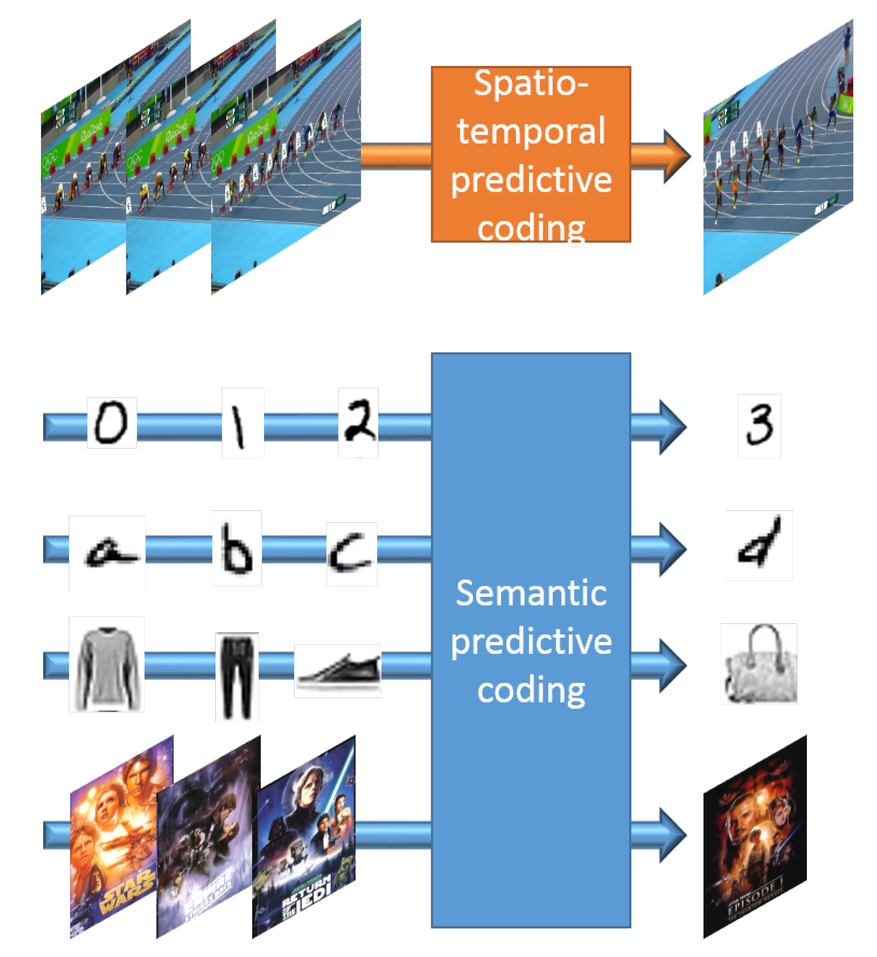
In this work, we lay the foundations for an alternative and unique approach to the problem of next-frame prediction, by formulating a methodology able to directly derive higher-level visual semantics from an ordered sequence of images, instead of a lower-level representation of what has been previously observed. An intuitive insight of the difference between the typical next-frame prediction scenario (denominated spatio-temporal predictive coding) and the concept of semantic predictive coding introduced in this work can be gained in Figure 1. The proposed framework, termed Arbitrated Generative Adversarial Network (A-GAN), constitutes an indisputable distinction from currently existing works in the next-frame prediction literature in the fact that, while in traditional approaches, the adopted model attempts to guess the most likely future from all plausible outcomes, primarily guided by the image dynamics of the previous frames, in our case the prediction of each subsequent image is solely based on the deeper understanding and the well-aimed interpretation of the interconnected visual semantics of the input sequence. Indicative applications include examples in anomaly detection, with the objective to detect whether a new sample is normal or not, and recommendation engines, where sequences of bought items can be utilized for predicting the next recommended item. In this scenario, images for clothes bought by a user could be potentially utilized by the proposed scheme in order to recommend matching, new clothing items. Furthermore, such a service could utilize the synthesized images in order to retrieve similar available items.
Motivated by this novel perspective on the problem of next-frame prediction and, to the best of our knowledge, by the lack of relevant works that contemplate this certain approach, we utilize the cutting-edge deep learning methodology of Generative Adversarial Networks (GANs) [13] to effectively tackle the issue at hand. In particular, the adopted model is adversarially trained and aptly arbitrated in an effort to reliably respond to incoming sequences of ordered inputs, by generating appropriate visual outputs that successfully match contextually and coherently what has been previously observed. We thoroughly investigate the issue at hand from a principal yet significantly informative viewpoint of numerical and alphabetical enumerations to validate the potential of this work. In short, the key contributions of this work include:
- The formulation of the semantic predictive coding paradigm as an extension of the traditional next-frame prediction paradigm.
- The development of a novel generative DNN architecture termed Arbitrated Generative Adversarial Networks for addressing the semantic predictive coding.
- The demonstration of the capabilities of the proposed framework on the visual prediction of alphanumeric sequences.
The rest of this paper is structured, as follows. In Section 2, we summarize the related work in spatio-temporal predictive coding with deep learning methodologies. In Section 3, we describe the utilized methodology and establish the proposed A-GAN framework. In Section 4, we present our experimental findings with accompanying discussion. Finally, conclusions about this work are deduced in Section 5.
2. Related Work
At present, a wide assortment of different deep learning methodologies has been developed, in an effort to address the problem of next-frame prediction, and have essentially flourished as the backbone of most video prediction approaches. The spatio-temporal nature of the problem has prompted the adoption of the three-dimensional (3D) convolutional operation in a variety of works [14,15,16], in an attempt not only to derive the inherent correlations in the spatial domain of each input frame, but also the temporal dynamics between subsequent frames. On the other hand, an alternative approach is presented in [17], where a combination of both a temporal encoder and an image generator is employed in the proposed GAN scheme, so as to successfully capture the underlying time series in the data.
Sequence models [18] and, in particular, certain variations of the Long Short Term Memory (LSTM) [2] archetype, have materialized as a significant component in the next-frame prediction literature. In [19], the authors implement a recurrent pyramid of stacked gated autoencoders [20], while Srivastava et al. [21] propose an alternative autoencoder-based architecture comprising an LSTM encoder and one or multiple LSTM decoders (one for the reconstruction of the input sequence and another for the prediction of future frames). The concept of the Convolutional-LSTM (ConvLSTM) is introduced for the first time in [22], a substantial extension of the fully-connected LSTM, with convolutional structures in both the input-to-state and state-to-state transitions. PredNet, an attempt for an in-depth and meticulous implementation of the brain’s predictive coding mechanisms is demonstrated in [23], while in [24] a thorough assessment of the same network is conducted, both in terms of the fidelity of the intended realization and of its potency for the problem at hand. In [25], the authors recommend the segregation of the video motion and content with the introduction of two different encoders, one for the image spatial information and another (LSTM) for motion dynamics. The combined knowledge from both can then be leveraged by a convolutional decoder in order to perform a more effective prediction. Finally with PredRNN [26], and the improved version of the same idea in [27], an enhanced memory cell for the LSTM architecture is proposed with the ability to derive both spatial and temporal representations at the same time.
The debut of GANs in the video prediction literature transpired in 2016 with the work of Mathieu et al. [28]. In this work, the authors acknowledge the disadvantage of the sole use of a pixel error-based loss (e.g. MSE), and they subsequently suggest the combined adoption of an adversarial-based loss, along with an image gradient difference loss and a conventional reconstruction error-based loss. A multi-scale architecture is also recommended in an effort to mitigate the loss of resolution resulted by the use of pooling. Ever since, a multitude of GAN-related works for next-frame prediction have emerged [29,30,31,32,33,34,35,36,37,38] demonstrating the grand potential of this cutting-edge methodology. At the same time, recent advances in the broader image generation literature, from image [39] and video [40] super resolution, semantic image synthesis [41,42,43] and image inpainting [44] to the generation of natural images [45], texture synthesis [46], and face generation [47,48], have consolidated GANs as the “belle of the ball" in a plethora of prominent tasks in the computer vision discipline. Moreover, other significant works concerning the GAN archetype are summarized below. In Mirza et al. [49], a conditional variation of the vanilla GAN framework is proposed. Contrary to the latter [13], where the imitated data distribution is exclusively generated from random noise, in this newly explored case both the generator and the discriminator can be conditioned on additional priorly available information, such as the class label of the provided input. The “Wasserstein” GAN is introduced in [50], where the exploitation of the Earth mover’s distance [51] is demonstrated to result in a more stable training process. Finally, with the concept of Coupled GANs (CoGAN) in [52], a joint distribution of multimodal images can be determined without the need to provide the network with matching images of both modalities at training time.
3. Proposed Methodology
In this paper, we employ state-of-the-art deep generative models in an effort to investigate the task of predictive coding from a new unexplored angle. While, in conventional video frame prediction, the generation of each subsequent frame is primarily centered around the understanding of the scene dynamics, in this work we attempt to ascertain the capability of the proposed model to derive meaningful visual semantics and semantic associations from ordered sequences of symbols. To properly examine and effectively address the semantic predictive coding task, we consider the state-of-the-art framework of GANs, introduced by I. Goodfellow et al. [13], which has paved the way for significant breakthroughs in a wide range of applications in the past few years. Its adoption in the typical scenario of the problem of next-frame prediction [28,34], as well as in a variety of tasks in the target-image generation literature [39,40,41], has demonstrated the auspicious capabilities of this deep generative modeling archetype.
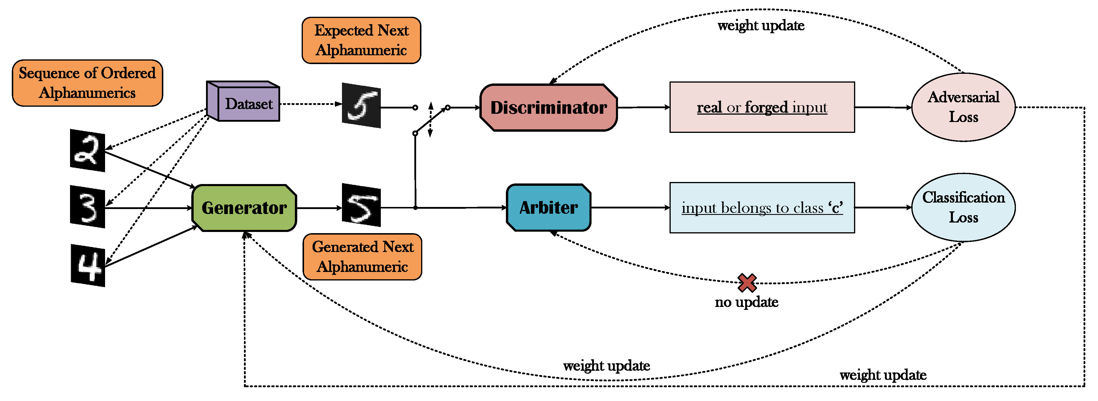
Further elaborated, the proposed framework introduces an alternative loss function in lieu of the -based losses commonly used, where instead of imposing a constraint on the reconstruction quality of the desired image output of the generator, a classification-based loss is adopted in accordance with the ground-truth class that encapsulates the output’s expected semantic content. Essentially, we accomplish this alteration by inserting an additional DNN to the GAN “equation”, along with the generator and the discriminator, which we refer to as the arbiter. The arbiter is a pre-trained, and thus not trainable internally in the GAN optimization, classifier that exclusively interacts with the generator and that is solely engaged with the task of evaluating the symbols created by the latter, resulting in an appropriate classification loss to be propagated back to the generator (Figure 2).
We focus on the specific scenario of the visual anticipation of succeeding fundamental alphanumeric symbols, when presented with an input sequence of either numerical digits or alphabetic characters in an ascending order. In both examples, the datasets that we employ are entirely based on the popular subsets of the NIST Special Database (https://www.nist.gov/srd/nist-special-database-19), namely the MNIST Database of Handwritten Digits (http://yann.lecun.com/exdb/mnist/) [53] and the EMNIST Letters (https://www.nist.gov/itl/products-and-services/emnist-dataset) [54].
3.1. Generative Adversarial Networks
The unveiling of the generative adversarial networks’ archetype occurred in 2014 by I. Goodfellow and his colleagues [13]. The principal idea incorporated in this vanilla GAN framework introduces two interplaying DNN adversaries, the generator (G) and the discriminator (D), which compete with each other in a game-theoretic approach. While the generator’s G: main purpose manifests in the realistic synthesis of image data observations of a certain distribution (based on an input latent variable , which is randomly drawn), at the same time, the discriminator’s D: principal task is to evaluate both real and synthesized samples, coming from the original distribution and from the generator respectively, and to determine their authenticity via a probability output. Ideally, for an image this probability output would be equal to 1, whereas for a synthesized image the probability would be 0. Vice versa, in the case of the generator, the ideal scenario would entail the exact opposite event of , given that G is expected to result in realistic and credible image observations in order to deceive D. Essentially, and as the game unfolds, both entities gain knowledge from each transpired outcome in an attempt to exploit what they have already learnt and to improve the quality of their results. This two-player minimax game between G and D can be described by the function:
where and correspond to the generator’s and the discriminator’s trainable parameters. In practice, both G and D are trained concurrently by alternating gradient updates.
The same fundamental idea can be easily attuned to the problem of next-frame prediction and, in particular, to the special case addressed in this work (Figure 2). In a similar manner to what has been previously described, the generator’s G: main task still remains the consistent imitation of image data observations originating from a certain distribution . Instead of a latent variable z, this time G receives an input of image symbols (digits or letters), ordered with respect to their semantic content, and with the primary objective to generate the correct succeeding symbol in the row. At the same time, the discriminator’s D: received input (image symbols either generated from G or originating from ) and derived output (probability of being real) are maintained as is. Given that we exclusively operate on either the MNIST Database of Handwritten Digits or the EMNIST Letters dataset, the spatial dimensions of each observation correspond to the values , while the channel dimension l is equal to 1. Finally, in the case of the loss function of Equation (1), it is accordingly transformed into the following:
3.2. Arbiter Network
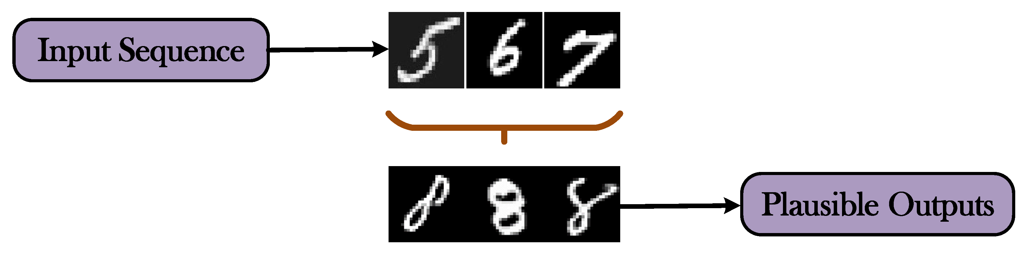
Even though the utilization of the conventional adversarially trained GAN architecture for the task of next-frame prediction can eventually lead to an exceptionally accurate imitation of the original data distribution, it nevertheless does not establish any concrete guarantees ascertaining that the generated output will ultimately be valid in terms of the continuity of the provided input sequence. In practice, and in accordance with the newly introduced scenario proposed in this work, not only G is required to deliver image symbols that will be outright indistinguishable from their legitimate counterparts, but, at the same time, it is imperative for a constraint to be set in order to ensure the coherent semantic association of the output’s content as a corollary to what has already been observed in the input. For example, when considering the input sequence illustrated in Figure 3, the generation of a corresponding image output depicting any numerical digit, except from ‘8’, would clearly satisfying the conditions defined by the adversarial loss for G, despite the fact that in reality none of these numbers correctly represent the desired outcome.
In the typical setting of next video frame prediction with GANs, and in a variety of target-image generation tasks, the adoption of an additional pixel error-based loss between the desired image output and its synthetic equivalent constitutes an effective and rational choice in the endeavor to impose the similarity between prediction and expectation. From the widely used -related losses in [28,39] to a feature space VGG [39,40] and the Charbonnier [40], this category of losses has demonstrated the vast potential of the GAN archetype in successfully addressing such demanding tasks. However, this rather straightforward workaround poses a significant disadvantage to the uniquely defined perspective of the semantic predictive coding. By concretizing the form of the expected next-in-line symbol, based on the content of the given input sequence, and by imposing a pixel-wise comparison with the generator’s predicted output, we consequently establish unnecessary limitations in the set of plausible outcomes, subdue G’s creativity, and impair its generalization capacity. The problem that arises related to the use of such a loss can be easily identified, in a simplistic context, by observing a subset of all the plausible outputs associated with the input sequence (‘5’, ‘6’, ‘7’) in Figure 3. Conceptually, we understand that the number ‘8’ is definitely the one that should follow, but which realization of an image of an ‘8’ would we choose to use on our loss function and why would we favour this choice over other valid candidates?
We propose a departure from the commonly used reconstruction error-based loss functions, which does not align well with the particular requirements of the introduced approach, and the utilization of a classification-based loss instead, in order to avoid this predicament. By formulating a simple labeling scheme that encapsulates appropriately the semantic content of each possible symbol, we can accomplish a pivotal transition from the concept of actualizing symbols with strict and inflexible requirements regarding their form to the realization of each new symbol with a much more abstract and conceptual approach. Thus, we avoid setting unnecessary limitations to the model on the form of the predicted outcome and, instead, we grant it carte blanche in order to operate in a more inventive and resourceful manner.
The introduction of the required classification loss can be effectively achieved by inserting an additional third network in the GAN architecture, along with the generator and the discriminator, denominated as the arbiter (A). The principal task that A: is appointed with, pertains to the assessment of the image samples that have been generated by G, in terms of the quality and the veracity of their semantic content. Essentially, A is none other than a high-accuracy pre-trained DNN classifier tasked to categorize images of the c distinct symbols classes of the employed dataset, 10 in the case of next-digit prediction, and 26 in the next-letter prediction scenario. If G manages to correctly (or incorrectly) predict the next image symbol, then A, in turn, will most probably result in an accurate (or inaccurate) categorization of this symbol, leading as such to a minuscule (or rather large) classification loss. On the other hand, there is no interaction between A and D, meaning that they both have a direct impact on the optimization of G’s generation procedure, but not on each other’s probability outcomes. In the case of the classification loss of the arbiter, we choose to adopt the widely used categorical cross-entropy loss, also known as softmax loss, which, given the typical one-hot-encoding labeling on most DNN classifiers, is defined as follows:
where corresponds to A’s output score (before softmax) for the true class and to the output score for the i-th class. As a final note, given that A is pre-trained and, thus, highly competent in the task it has been assigned to, there is no need to be further trained internally in the GAN, meaning that it completely ignores the backpropagated gradients exploited by G to optimize its generative capabilities.
3.3. The A-GAN Framework
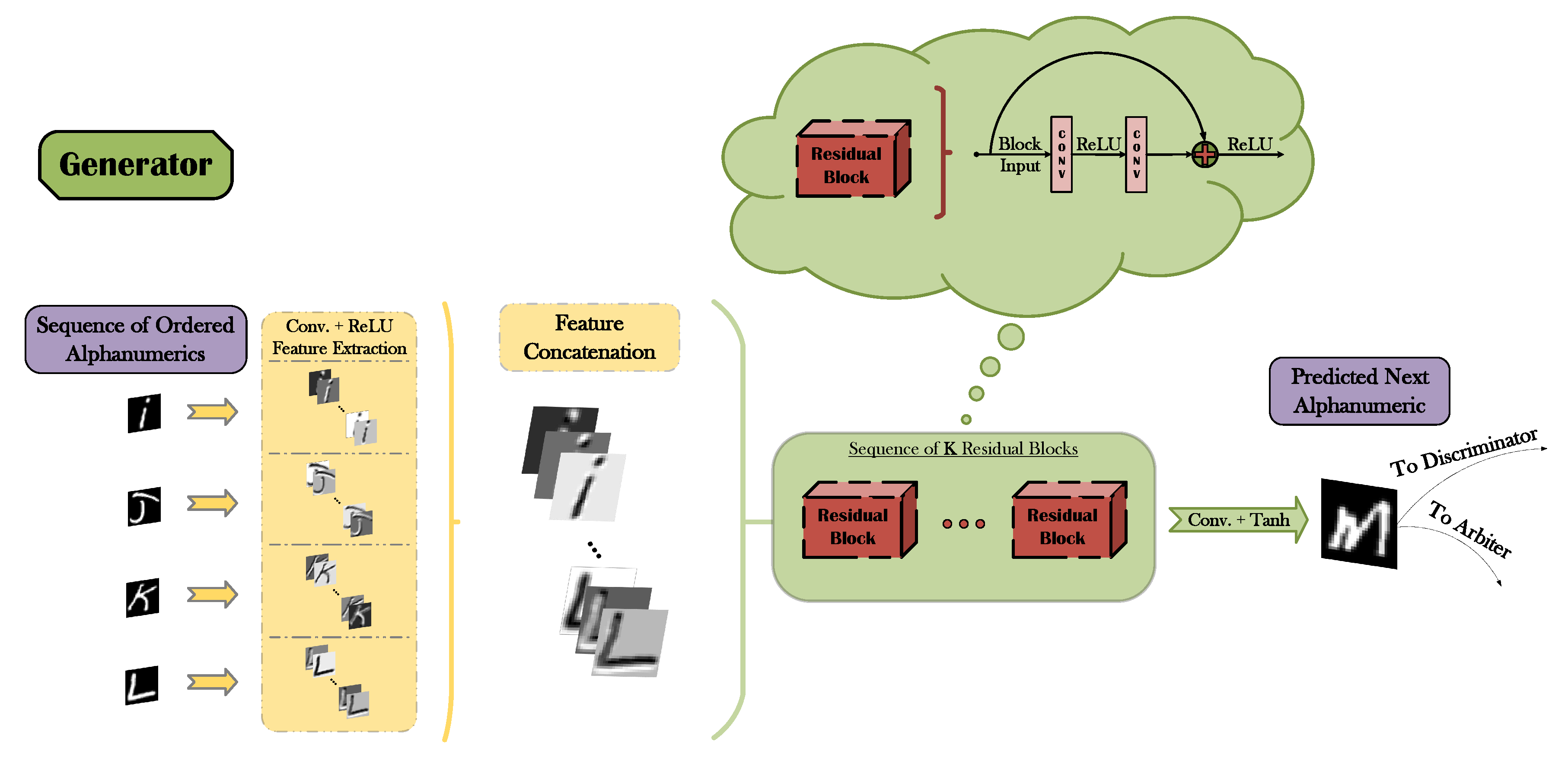
The block diagrams presented in Figure 4 (generator) and Figure 5 (discriminator and arbiter) broadly present the main functionalities of the three DNNs that comprise the proposed A-GAN architecture. As illustrated in Figure 4, G initially receives an input sequence of symbols in ascending order, it concurrently extracts relevant representations independently for each symbol (via the combination of convolutional filters and the ReLU [55,56] activation) and it concatenates the resulting feature maps into a unified tensor of features. A deep residual network [4] with K residual blocks (where K is a hyperparameter) then operates on the derived tensor ultimately leading to a visual prediction of the next symbol in line. Given that the employed image datasets have been pre-processed and normalized in the value range of , the hyperbolic tangent (tanh) function is utilized as an appropriate activation output of the network. Even though the aformentioned pipeline corresponds to the training phase of the generator, still it is retained unaltered during inference.
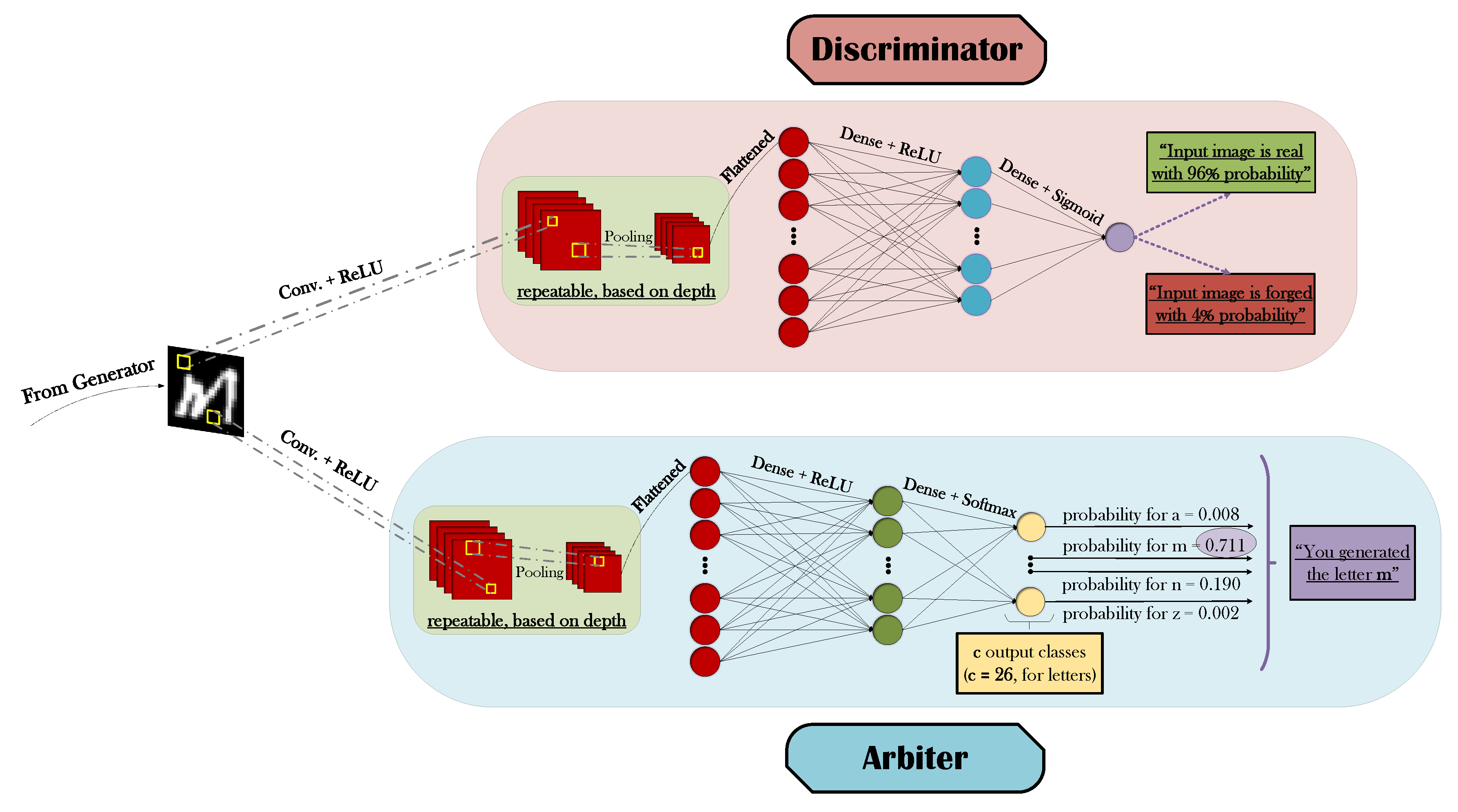
The synthesized images that have been generated by G are simultaneously processed by both D and A, as easily observed in Figure 5. The conventional yet very powerful methodology of Deep Convolutional Neural Networks (DCNNs or CNNs) [3,57] has been selected as the basis for both classifiers, with a combination of convolutional + ReLU feature extractors, pooling operations, and fully-connected layers essentially culminating in the corresponding predictions. The principal distinction between D’s and A’s CNN architectures materializes in the size and activation choice of their respective final layers, having in mind that the former is a binary and the latter a multi-class classifier. For every generated symbol, and for each corresponding real image equivalent that D is presented with, a binary decision regarding their authenticity must essentially be made. Thus, a single output unit with a sigmoid activation will suffice in deriving an associated probability value of whether the observed input is actually real or forged. On the other hand, given that A’s main task amounts to the reliable categorization of the synthesized input’s semantic content into c mutually exclusive classes, then a final layer of c different output units with a softmax transfer function constitute the de facto choices. Even though both softmax and sigmoid result in probability-oriented outputs, the critical advantage of the former is that it reflects a normalized probability for each class, constraining the sum of all probability values to add up to one. Thus, while A’s confidence for the prediction of a specific class strengthens (hopefully the true class), it affects not only the corresponding probability for that class that will obviously increase, but also the respective probability values for the remaining classes that will have to decrease.
As a final note, we define the combined loss function used for the generator’s training, consisting of an adversarial loss and of the arbiter loss, as already described in Equations (2) and (3), respectively. Given that is generally prone to saturation, we choose to minimize instead. Therefore, for a given training input sequence and an output score of the succeeding element’s ground-truth class, the combined loss becomes:
where and are weight factors for each loss term.
4. Experimental Analysis and Discussion
4.1. Dataset Manipulation
The MNIST Database of Handwritten Digits [53] and the EMNIST Letters dataset [54] have been utilized for the performance evaluation of the proposed methodology. Both of the datasets have been pre-processed and normalized in the value range of and have been split into two complement subsets, the training and the test set. For each experimental setup, the input of the generator exclusively consists either of digit or letter sequences of length t. Given a batch size b and a number of training iterations i, the total number of training sequences can be calculated as . Each of the input sequences, both during training and at inference, is dynamically created by randomly selecting an initial symbol as a starting point and by additionally appending its succeeding elements from the corresponding dataset. Among the symbols of the same semantic content, each selection is performed at random. For example, and for , consider a training input sequence of digits that we randomly select to start with the number ‘5’. From all the different training images that depict the number ‘5’, we arbitrarily pick one as the starting point of the sequence. Then, we select, also by random, one image per each subsequent element, namely the numbers ‘6’, ‘7’, and ‘8’. Lastly, given that, in reality, the digit ‘9’ and the letter ‘z’ are terminal, then for the sake of our experiments we assume a circular ordering, meaning that we regard the digit ‘0’ as the succeeding symbol of ‘9’ and the letter ‘a’ as the next-in-line after ‘z’.
4.2. Experimental Setup
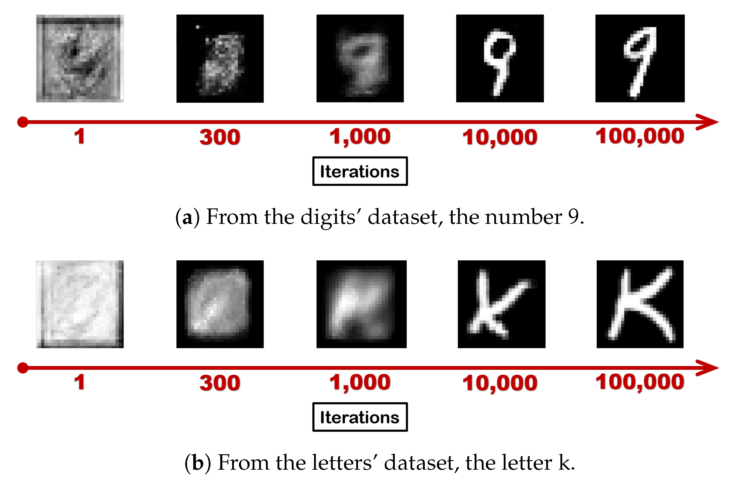
Each experimental setup has been trained for 100,000 iterations with a batch size of 10, resulting in 1,000,000 different training input sequences. At the same time, 10,000 test sequences have been utilized for the evaluation of each model. Figure 6 depicts an example of the evolution of the generation procedure with regard to the training iterations. The performance of the proposed approach in the case of the digits’ dataset has been investigated with a separately trained A-GAN from that of the letter’s dataset. In both cases, extensive hyperparameter tuning has been conducted and the experimental findings have suggested the following setup as the optimal layout of each demonstrated network. Regarding G’s initial feature extraction stage, 128 different convolutional kernels have been trained per each symbol in the input sequence, totaling to feature maps in the concatenation stage. Subsequently, the utilization of 15 residual blocks with 128 different filters per convolutional operation has been designated as the optimal architectural choice in the case of the residual network. For D, two convolutional layers have been selected with 64 and 128 filters respectively, one dense-ReLU layer with 1024 neuronal units and a dense-sigmoid layer with 1 unit. Max pooling has been also applied after each convolutional layer. Finally, A has been pre-trained independently from G and D with three convolutional layers of 64, 128, and 256 filters, max pooling, one dense-ReLU layer of 512 units, and a dense-sigmoid layer with either 10 output units, in the digits’ scenario, or 26 units in the case of the letters. The utilization of a dropout [58], applied exclusively on the dense layers, has demonstrated an enhanced performance in the case of A, but it has not yielded any better results in the case of G and D. Batch normalization [59] has been adopted in all three networks. As for the weight factors and of the loss terms in Equation (4) it has been determined that a value of , in the case of the next-digit prediction, and values of and , in the next-letter prediction, should essentially result in the best performance. As a final note, in the majority of our experimental efforts we have mainly focused on input sequences of length , but we have also examined alternative cases in Section 4.3.2.
4.3. Qualitative and Quantitative Results
A thorough investigation of the various aspects of the problem at hand must be conducted leading to handily interpretable experimental findings of both qualitative and quantitative nature in order to effectively perform a comprehensive evaluation of the potential of the proposed approach. Given the higher-level perspective of the problem, as compared to the conventional scenario of video prediction, the most evident and indisputable way of assessing the quality of the derived results is by visually inspecting each corresponding prediction. For instance, characteristic examples of fitting predictions that have been generated by concretely trained models can be observed in Figure 7. On the other hand, there is not a straightforward and unambiguous way to sufficiently measure the performance of this approach, in comparison with the typical evaluation metrics used in other target-image generation tasks including the Peak Signal to Noise Ratio (PSNR) and the Structural Similarity Index Measure (SSIM) [60]. To this end, we propose the utilization of the arbiter not only as a regulator of the optimization of G’s generative capabilities, but also as a critical assessor for the quantification of G’s predictive potency during inference. As we have already stated, A is a highly-competent classifier of digits or letters (based on the context of the data), whose status remains unaltered during the training of the GAN. After the completion of the training procedure, we need to effectively evaluate in a measurable and direct way the performance of G, when presented with new unseen input sequences. Given that, for each new sequence, G must respond with a visual prediction of the supposed next element, subsequently this prediction can be fed-forward to A in order to categorize it into an existing class. If we compare A’s output with the class label that essentially corresponds to the desired semantic content of the predicted element, this would result in a classification accuracy measure as a quantifiable criterion of the performance of G, as follows:
where is the number of G’s generated predictions correctly classified by A and is the total number of predictions.
4.3.1. Chains of Consecutive Predictions
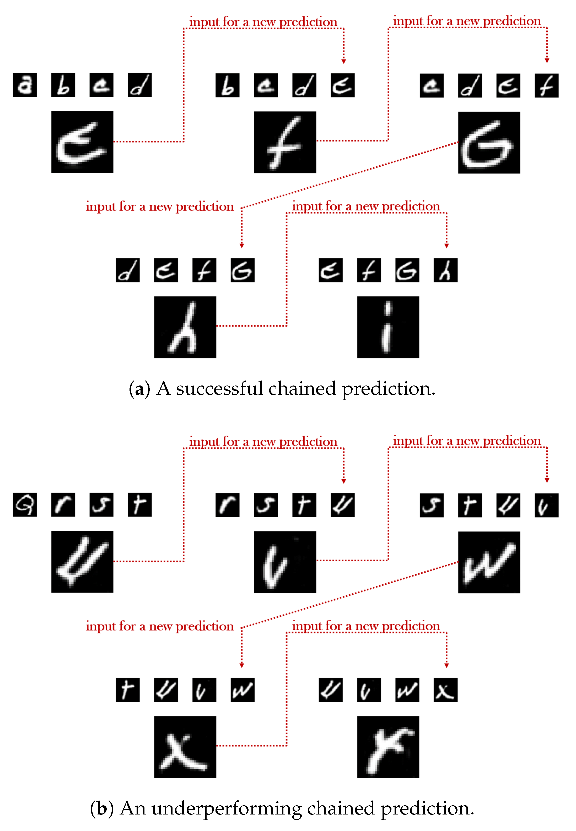
The evaluation of a model that is based on the generation of a single next-frame can be partially indicative of the model’s high or limited potential in tacking the problem at hand, but it can also prove misleading if no further examination of its predictive potency is conducted. This evaluation can be easily extended to a chain of consecutive predictions during inference to be able to separate the wheat from the chaff. In particular, for each link of a chain, G’s current output can be essentially circulated back into the network as part of the input sequence, thus triggering a new prediction. This way, the performance of each model can be thoroughly assessed through a multi-stage procedure, enabling a tangible distinction between a consistently highly-achieving model and a model with an ostensibly prominent performance that will eventually fall apart somewhere along the chain.
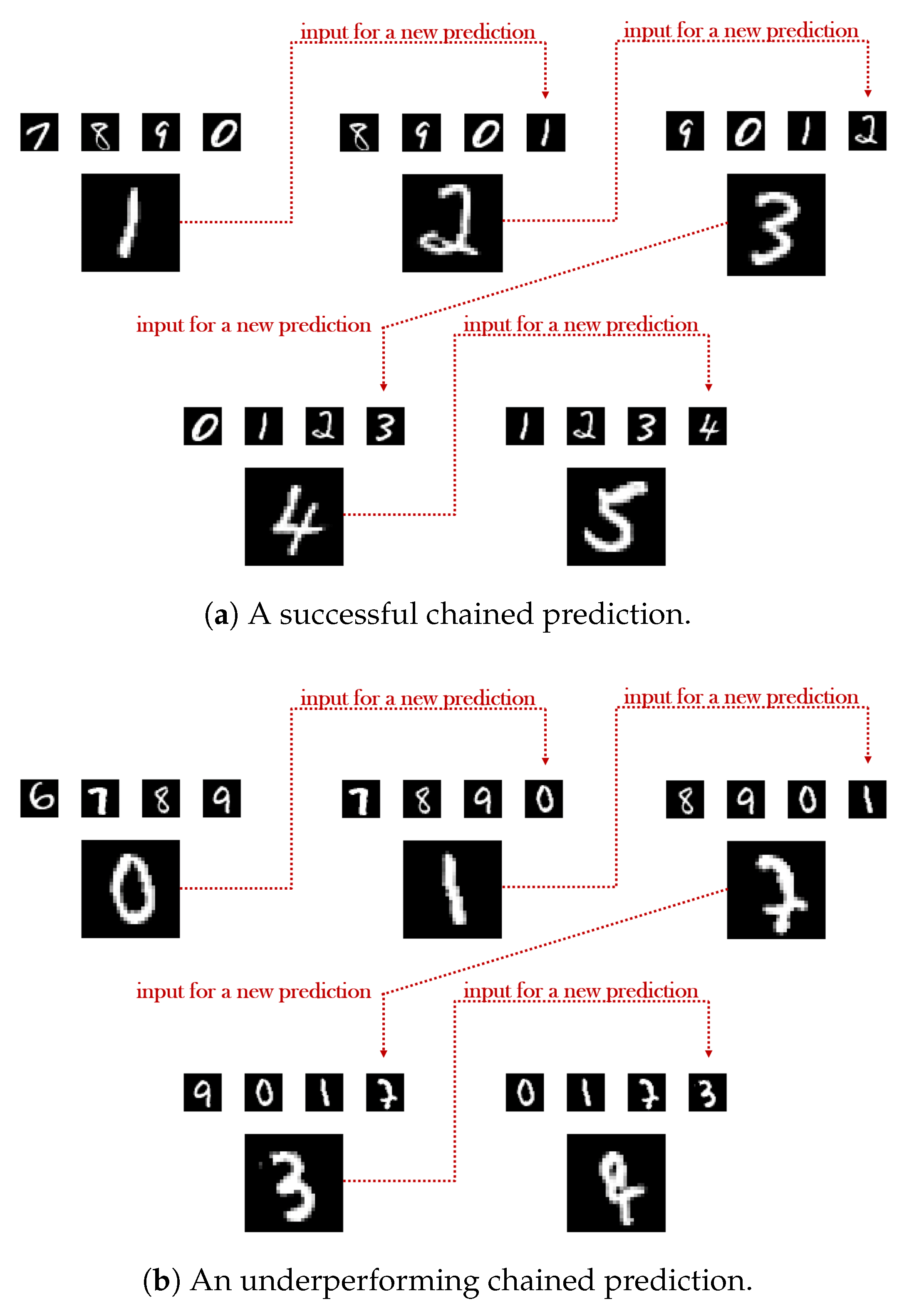
A characteristic example supporting the aformentioned analysis is demonstrated in Table 1 in the case of the digits’ dataset. As easily observed, even though the two contrasted models do not differ significantly in terms of the resulted accuracy in the first link of the chain (), as we move deeper, the second model falls short of the expectations with a sharp accuracy decrease ( from the first to the fifth link) broadening the gap between the two to . A brief qualitative comparison of the two models is also conducted in Figure 8, where the underperforming case yields failed predictions in the 3rd and in the 5th link of the chain. Even though in the 3rd, the correct succeeding element of the given input sequence (‘8’, ‘9’, ‘0’, ‘1’) is arguably the digit ‘2’, instead, the generated output has been categorized as a ‘7’ by A. At the same time, in the case of the 5th link, the quality of the predicted image is once again inadequate, something that can be also backed by the arbiter’s wrongful categorization which has resulted in the class ‘8’.
In a similar manner, an additional quantitative comparison in the next-letter prediction scenario is presented in Table 2, where the initial accuracy difference of of the two models is eventually escalated into a substantial . Furthermore, in Figure 9, the inferiority of the quality of the underperforming model’s generated results is evidently validated by the ambiguity in their forms, leading to an increased uncertainty in A’s predictions almost everywhere in the chain. For example, even though the derived letter ‘v’ in the second link is correctly classified as such by A, the corresponding probability for the class ‘v’ is still significantly low and, in fact, not far in value from that of the letter ‘c’, while in the 5th link of the chain, the expected ‘y’ class is mistakenly identified as ‘x’.
4.3.2. Impact of the Cardinality of the Input Sequence
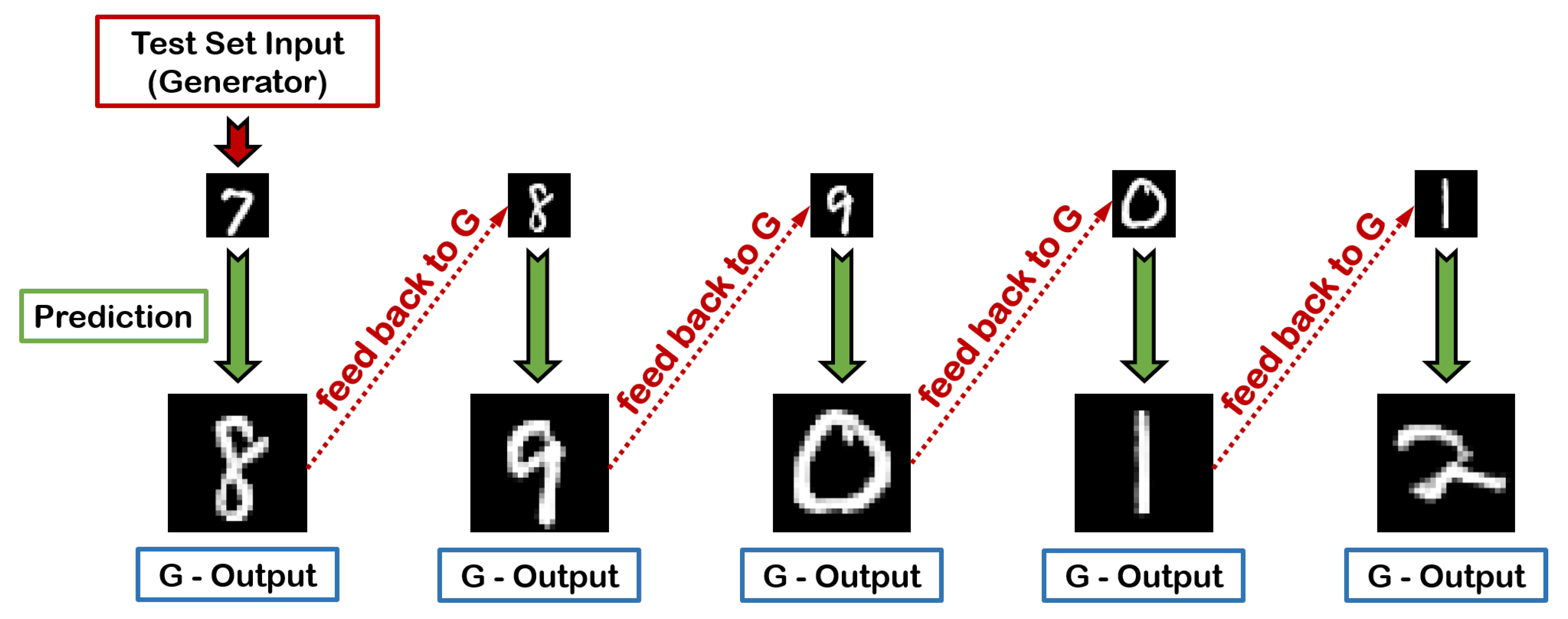
In this subsection, we explore the impact of the input’s cardinality t in G’s predictive performance, as an attempt to address the question of how many symbols are, in fact, sufficient to form a reliable decision on what will be essentially observed next. The first and most evident deduction that can be made by observing Table 3 (digits) and Table 4 (letters) is the fact that, when the cardinality of the input sequence decreases, a subsequent decline in the performance of the trained A-GAN is also witnessed. This can be easily explained taking into account that as t drops, not only the network’s prediction is based on a continuously reduced amount of information, but also becomes more uncertain, given that the ratio of real data to the generated data in the input also decreases moving deeper into each chain. For example, for , this ratio is 4:0 in the first link, 3:1 in the second, and 2:2 in the third, while for this ratio becomes 3:0, 2:1, and 1:2, respectively. In the extreme case of , as illustrated in Figure 10, each prediction in the chain is exclusively performed with single-image inputs, meaning that, apart from the first link where the input originates from the test dataset, for deeper links the input is purely synthetic and exclusively based on the corresponding output feedback from each preceding link.
An equally important observation can be expressed in the comparison between the two employed datasets, where the utilization of a shorter sequence of input symbols in the next-letter anticipation scenario appears to have a severely greater impact in the performance deterioration of the trained A-GAN in contrast to the next-digit prediction. An intuitive explanation to this phenomenon stems from the fact that in the case of the letters’ dataset, not only the labelset of possible classes is significantly larger as compared to the digits (26 to 10), but there is also a greater diversity in characters of the same class, given the concurrent existence of both capital and lower-case letters in EMNIST. The highest performance drop of , from to , in the 5th link of the chain in the digits’ scenario, still remains a smoother decrease when compared to the in the first link and the drop in the fifth link in the letters’ case.
4.3.3. Arbiter’s Loss Versus Loss
A final, yet very critical, evaluation criterion for the introduced A-GAN framework materializes in the comparison of the proposed arbiter’s classification loss (Equation (3)) versus a conventional, and commonly used in various target-image generation tasks, pixel error-based loss. Given a non-arbitrated GAN with an loss, essentially we get the combined -GAN loss, as follows:
where is a reference image that is randomly chosen from the training dataset, independently for each training input sequence and in conformity with the semantic content of the true next element of the sequence. For example, and for , given an input sequence of the letters (‘e’, ‘f’, ‘g’), then the true next symbol is the letter ‘h’. Thus, we arbitrarily select a random image of the letter ‘h’ from the training dataset to contribute in the calculation of the loss in conjunction with the generated prediction. Instead of designating a constant, across all training iterations, reference image per distinct symbol in the dataset, we choose the random selection strategy in an effort to secure a potentially better variability in the results of .
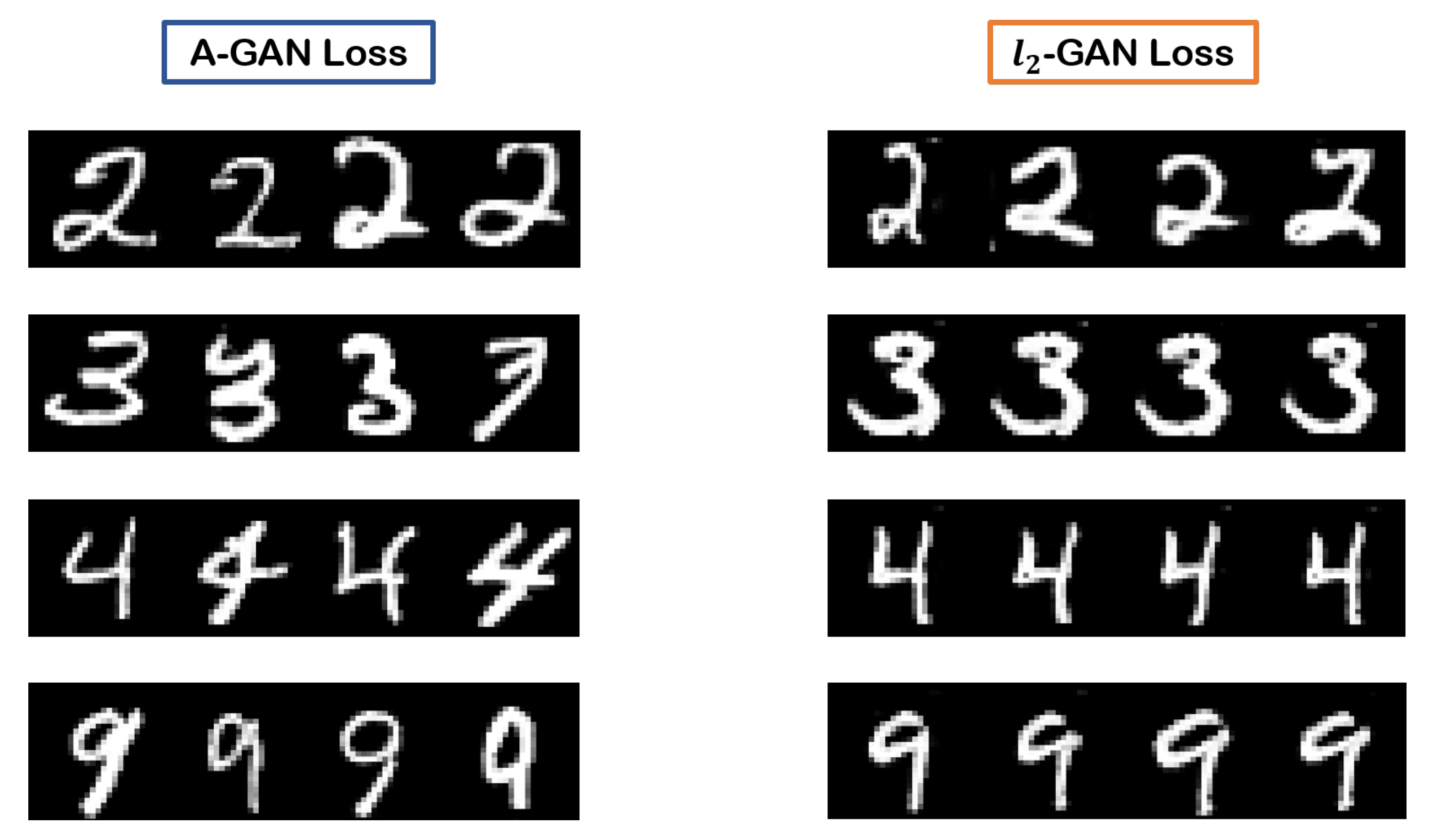
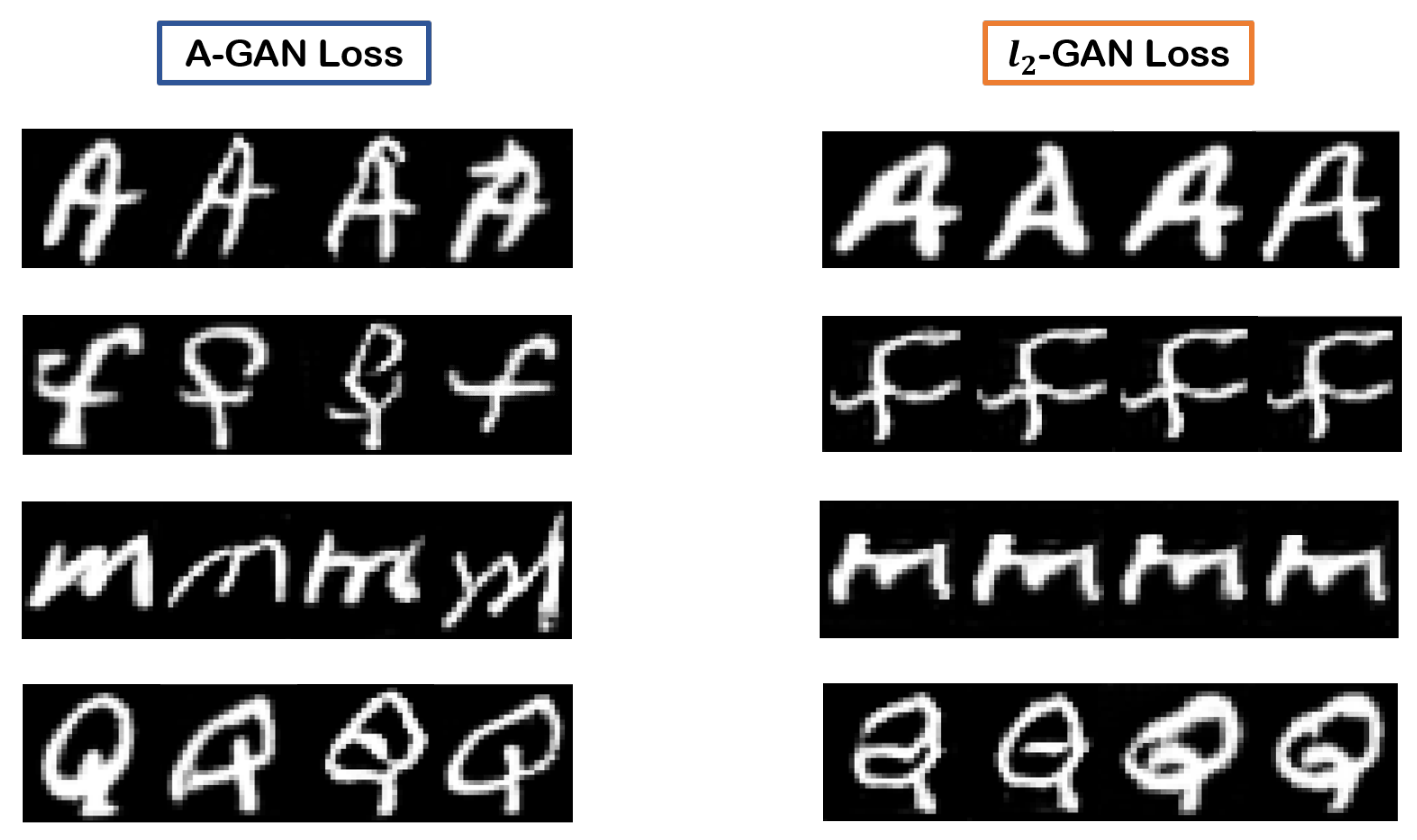
Characteristic examples of correctly predicted symbols during inference are illustrated in Figure 11 (digits) and Figure 12 (letters), for both the A-GAN and -GAN. The clear advantage of the proposed arbitrated methodology is validated in the two Figures, both in terms of the quality and the diversity of the derived images. Even though the -GAN is capable of generating decent results with regard to the veracity of their content, there is no significant variation in the symbol forms, with a collateral development of some pixel artifacts in the cases of the digits ‘2’, ‘3’, and ‘4’ in Figure 11. The superiority of the proposed approach is also confirmed in quantifiable terms in Table 5, where, in the digits’ scenario, the A-GAN overpowers the -GAN from accuracy in the first link of the chain to in the fifth link, with a respective to increased performance in the case of the letters.
5. Conclusions
In this paper, we proposed an alternative approach to the problem of next-frame prediction, termed semantic predictive coding. Marking a departure from the typical example of spatio-temporal video prediction, we instead focused on sequential images that follow a certain form of associative ordering. In our approach, instead of drawing inferences that are based on the spatial information and the temporal dynamics of past frames, we take advantage of the semantic information concealed in the data in an effort to contextually guess the next element. To effectively address this issue, we adopted a novel variation of the conventional GAN architecture, denominated Arbitrated Generative Adversarial Networks (A-GANs). In particular, we introduced an additional DNN, termed the arbiter, in the GAN ecosystem, responsible for the assessment of the reliability of the generated visual outputs based on the designated class that they are naturally expected to belong. The arbiter is able to provide a classification-based loss that is associated with each generated image, in contrast to the reconstruction-based losses that are most commonly used in other cases where the desired visual output is known during the training procedure. We thoroughly evaluated the capabilities of the proposed approach in two scenarios, one for the next-digit and one for the next-letter prediction. The introduction of the arbiter as an essential overseer of the validity of the generation process, not only constitutes a novel approach in the GANs’ target-image generation and next-frame prediction literature, but it is also demonstrated to achieve high in quality and creative results. Future work will be focused on the application and evaluation of the proposed approach in other scientific disciplines.
Author Contributions
Conceptualization, R.S., G.T., P.T.; methodology, R.S., G.T., P.T.; software, R.S.; formal analysis, R.S., G.T., P.T.; writing—original draft preparation, R.S.; writing—review and editing, G.T., P.T.; visualization, R.S.; supervision, G.T., P.T.; project administration, P.T.; funding acquisition, P.T. All authors have read and agreed to the published version of the manuscript.
Funding
This research work was funded by the Hellenic Foundation for Research and Innovation (HFRI) and the General Secretariat for Research and Technology (GSRT), under HFRI faculty grant no. 1725, and by the Stavros Niarchos Foundation within the framework of the project ARCHERS (Advancing Young Researchers’ Human Capital in Cutting Edge Technologies in the Preservation of Cultural Heritage and the Tackling of Societal Challenges).
Acknowledgments
The authors would like to thank Michail-Eleftherios Spanakis for his contribution.
Conflicts of Interest
The authors declare no conflict of interest.
Abbreviations
The following abbreviations are used in this manuscript:
| GAN(s) | Generative Adversarial Network(s) |
| AI | Artificial Intelligence |
| DNN(s) | Deep Neural Network(s) |
| A-GAN | Arbitrated Generative Adversarial Network |
| LSTM | Long Short Term Memory |
| ConvLSTM | Convolutional-LSTM |
| MSE | Mean Squared Error |
| CoGAN | Coupled Generative Adversarial Network |
| NIST | National Institute of Standards and Technology |
| MNIST | Modified NIST |
| EMNIST | Extended MNIST |
| VGG | Visual Geometry Group |
| ReLU | Rectified Linear Unit |
| (D)CNN(s) | (Deep) Convolutional Neural Network(s) |
| PSNR | Peak Signal to Noise Ratio |
| SSIM | Structural Similarity Index Measure |
References
- LeCun, Y.; Bengio, Y.; Hinton, G. Deep learning. Nature 2015, 521, 436–444. [Google Scholar] [CrossRef] [PubMed]
- Hochreiter, S.; Schmidhuber, J. Long short-term memory. Neural Comput. 1997, 9, 1735–1780. [Google Scholar] [CrossRef] [PubMed]
- Krizhevsky, A.; Sutskever, I.; Hinton, G.E. Imagenet classification with deep convolutional neural networks. In Proceedings of the Advances in Neural Information Processing Systems, Lake Tahoe, NV, USA, 3–6 December 2012; pp. 1097–1105. [Google Scholar]
- He, K.; Zhang, X.; Ren, S.; Sun, J. Deep residual learning for image recognition. In Proceedings of the IEEE Conference on Computer Vision and Pattern Recognition, Las Vegas, NV, USA, 27–30 June 2016; pp. 770–778. [Google Scholar]
- Rumelhart, D.E.; Hinton, G.E.; Williams, R.J. Learning Internal Representations by Error Propagation; Technical report; California University San Diego, La Jolla Institute for Cognitive Science: San Diego, CA, USA, 1985. [Google Scholar]
- Srinivasan, M.V.; Laughlin, S.B.; Dubs, A. Predictive coding: A fresh view of inhibition in the retina. Proc. R. Soc. Lond. Ser. B Biol. Sci. 1982, 216, 427–459. [Google Scholar]
- Ballard, D.H.; Hinton, G.E.; Sejnowski, T.J. Parallel visual computation. Nature 1983, 306, 21–26. [Google Scholar] [CrossRef] [PubMed]
- Rao, R.P.; Ballard, D.H. Predictive coding in the visual cortex: A functional interpretation of some extra-classical receptive-field effects. Nat. Neurosci. 1999, 2, 79–87. [Google Scholar] [CrossRef] [PubMed]
- Friston, K.; Kiebel, S. Predictive coding under the free-energy principle. Philos. Trans. R. Soc. B Biol. Sci. 2009, 364, 1211–1221. [Google Scholar] [CrossRef] [PubMed] [Green Version]
- Bastos, A.M.; Usrey, W.M.; Adams, R.A.; Mangun, G.R.; Fries, P.; Friston, K.J. Canonical microcircuits for predictive coding. Neuron 2012, 76, 695–711. [Google Scholar] [CrossRef] [PubMed] [Green Version]
- Friston, K. Does predictive coding have a future? Nat. Neurosci. 2018, 21, 1019–1021. [Google Scholar] [CrossRef] [PubMed]
- Zhou, Y.; Dong, H.; El Saddik, A. Deep Learning in Next-Frame Prediction: A Benchmark Review. IEEE Access 2020, 8, 69273–69283. [Google Scholar] [CrossRef]
- Goodfellow, I.; Pouget-Abadie, J.; Mirza, M.; Xu, B.; Warde-Farley, D.; Ozair, S.; Courville, A.; Bengio, Y. Generative adversarial nets. In Proceedings of the Advances in Neural Information Processing Systems, Montreal, QC, Canada, 8–13 December 2014; pp. 2672–2680. [Google Scholar]
- Vondrick, C.; Pirsiavash, H.; Torralba, A. Generating videos with scene dynamics. In Proceedings of the Advances in Neural Information Processing Systems, Barcelona, Spain, 5–10 September 2016; pp. 1–9. [Google Scholar]
- Tulyakov, S.; Liu, M.Y.; Yang, X.; Kautz, J. Mocogan: Decomposing motion and content for video generation. In Proceedings of the IEEE Conference on Computer Vision and Pattern Recognition, Salt Lake City, UT, USA, 18–23 June 2018; pp. 1526–1535. [Google Scholar]
- Wang, Y.; Jiang, L.; Yang, M.H.; Li, L.J.; Long, M.; Fei-Fei, L. Eidetic 3D lstm: A model for video prediction and beyond. In Proceedings of the International Conference on Learning Representations, New Orleans, LA, USA, 6–9 May 2019. [Google Scholar]
- Saito, M.; Matsumoto, E.; Saito, S. Temporal generative adversarial nets with singular value clipping. In Proceedings of the IEEE International Conference on Computer Vision, Venice, Italy, 22–27 October 2017; pp. 2830–2839. [Google Scholar]
- Rumelhart, D.E.; Hinton, G.E.; Williams, R.J. Learning representations by back-propagating errors. Nature 1986, 323, 533–536. [Google Scholar] [CrossRef]
- Michalski, V.; Memisevic, R.; Konda, K. Modeling deep temporal dependencies with recurrent grammar cells. In Proceedings of the Advances in Neural Information Processing Systems, Montreal, QC, Canada, 8–13 December 2014; pp. 1925–1933. [Google Scholar]
- Memisevic, R. Learning to relate images. IEEE Trans. Pattern Anal. Mach. Intell. 2013, 35, 1829–1846. [Google Scholar] [CrossRef] [PubMed]
- Srivastava, N.; Mansimov, E.; Salakhudinov, R. Unsupervised learning of video representations using lstms. In Proceedings of the 32nd International Conference on Machine Learning, Lille, France, 6–11 July 2015; pp. 843–852. [Google Scholar]
- Xingjian, S.; Chen, Z.; Wang, H.; Yeung, D.Y.; Wong, W.K.; Woo, W.c. Convolutional LSTM network: A machine learning approach for precipitation nowcasting. In Proceedings of the Advances in Neural Information Processing Systems, Montreal, QC, Canada, 7–12 December 2015; pp. 802–810. [Google Scholar]
- Lotter, W.; Kreiman, G.; Cox, D. Deep predictive coding networks for video prediction and unsupervised learning. In Proceedings of the International Conference on Learning Representations, Toulon, France, 24–26 April 2017; pp. 1–18. [Google Scholar]
- Rane, R.P.; Szügyi, E.; Saxena, V.; Ofner, A.; Stober, S. PredNet and Predictive Coding: A Critical Review. In Proceedings of the 2020 International Conference on Multimedia Retrieval, Dublin, Ireland, 8–11 June 2020; pp. 233–241. [Google Scholar]
- Villegas, R.; Yang, J.; Hong, S.; Lin, X.; Lee, H. Decomposing motion and content for natural video sequence prediction. In Proceedings of the International Conference on Learning Representations, Toulon, France, 24–26 April 2017; pp. 1–22. [Google Scholar]
- Wang, Y.; Long, M.; Wang, J.; Gao, Z.; Philip, S.Y. Predrnn: Recurrent neural networks for predictive learning using spatiotemporal lstms. In Proceedings of the Advances in Neural Information Processing Systems, Long Beach, CA, USA, 4–9 December 2017; pp. 879–888. [Google Scholar]
- Wang, Y.; Gao, Z.; Long, M.; Wang, J.; Yu, P.S. Predrnn++: Towards a resolution of the deep-in-time dilemma in spatiotemporal predictive learning. In Proceedings of the 35th International Conference on Machine Learning, Stockholm, Sweden, 10–15 July 2018; pp. 5123–5132. [Google Scholar]
- Mathieu, M.; Couprie, C.; LeCun, Y. Deep multi-scale video prediction beyond mean square error. In Proceedings of the International Conference on Learning Representations, ICLR 2016, San Juan, Puerto Rico, 2–4 May 2016; pp. 1–14. [Google Scholar]
- Radford, A.; Metz, L.; Chintala, S. Unsupervised representation learning with deep convolutional generative adversarial networks. In Proceedings of the International Conference on Learning Representations, ICLR 2016, San Juan, Puerto Rico, 2–4 May 2016; pp. 1–16. [Google Scholar]
- Lotter, W.; Kreiman, G.; Cox, D. Unsupervised learning of visual structure using predictive generative networks. In Proceedings of the International Conference on Learning Representations, ICLR 2016, San Juan, Puerto Rico, 2–4 May 2016. [Google Scholar]
- Zhou, Y.; Berg, T.L. Learning temporal transformations from time-lapse videos. In Proceedings of the European Conference on Computer Vision, ECCV 2016, Amsterdam, The Netherlands, 11–14 October 2016; pp. 262–277. [Google Scholar]
- Liang, X.; Lee, L.; Dai, W.; Xing, E.P. Dual motion GAN for future-flow embedded video prediction. In Proceedings of the IEEE International Conference on Computer Vision, Venice, Italy, 22–29 October 2017; pp. 1744–1752. [Google Scholar]
- Lu, C.; Hirsch, M.; Scholkopf, B. Flexible spatio-temporal networks for video prediction. In Proceedings of the IEEE Conference on Computer Vision and Pattern Recognition, Honolulu, HI, USA, 21–26 July 2017; pp. 6523–6531. [Google Scholar]
- Vondrick, C.; Torralba, A. Generating the future with adversarial transformers. In Proceedings of the IEEE Conference on Computer Vision and Pattern Recognition, Honolulu, HI, USA, 21–26 July 2017; pp. 1020–1028. [Google Scholar]
- Bhattacharjee, P.; Das, S. Temporal coherency based criteria for predicting video frames using deep multi-stage generative adversarial networks. In Proceedings of the Advances in Neural Information Processing Systems, Long Beach, CA, USA, 4–9 December 2017; pp. 4268–4277. [Google Scholar]
- Wichers, N.; Villegas, R.; Erhan, D.; Lee, H. Hierarchical long-term video prediction without supervision. In Proceedings of the 35th International Conference on Machine Learning, ICML 2018, Stockholm, Sweden, 10–15 July 2018. [Google Scholar]
- Kwon, Y.H.; Park, M.G. Predicting future frames using retrospective cycle gan. In Proceedings of the IEEE Conference on Computer Vision and Pattern Recognition, Long Beach, CA, USA, 15–21 June 2019; pp. 1811–1820. [Google Scholar]
- Aigner, S.; Körner, M. FUTUREGAN: Anricipating the future frames of video sequences using spatio-temporal 3D convolutions in progressively growing gans. ISPRS Int. Arch. Photogramm. Remote Sens. Spat. Inf. Sci. 2019, XLII-2/W16, 3–11. [Google Scholar] [CrossRef] [Green Version]
- Ledig, C.; Theis, L.; Huszár, F.; Caballero, J.; Cunningham, A.; Acosta, A.; Aitken, A.; Tejani, A.; Totz, J.; Wang, Z.; et al. Photo-realistic single image super-resolution using a generative adversarial network. In Proceedings of the Proceedings of the IEEE Conference on Computer Vision and Pattern Recognition, Honolulu, HI, USA, 21–26 July 2017; pp. 4681–4690. [Google Scholar]
- Lucas, A.; Lopez-Tapia, S.; Molina, R.; Katsaggelos, A.K. Generative adversarial networks and perceptual losses for video super-resolution. IEEE Trans. Image Process. 2019, 28, 3312–3327. [Google Scholar] [CrossRef] [PubMed] [Green Version]
- Reed, S.; Akata, Z.; Yan, X.; Logeswaran, L.; Schiele, B.; Lee, H. Generative adversarial text to image synthesis. In Proceedings of the 33rd International Conference on Machine Learning, ICML, New York, NY, USA, 20–22 June 2016. [Google Scholar]
- Zhang, H.; Xu, T.; Li, H.; Zhang, S.; Wang, X.; Huang, X.; Metaxas, D.N. Stackgan: Text to photo-realistic image synthesis with stacked generative adversarial networks. In Proceedings of the IEEE International Conference on Computer Vision, Venice, Italy, 22–29 October 2017; pp. 5907–5915. [Google Scholar]
- Liu, X.; Meng, G.; Xiang, S.; Pan, C. Semantic image synthesis via conditional cycle-generative adversarial networks. In Proceedings of the 2018 24th International Conference on Pattern Recognition (ICPR), IEEE, Beijing, China, 20–24 August 2018; pp. 988–993. [Google Scholar]
- Pathak, D.; Krahenbuhl, P.; Donahue, J.; Darrell, T.; Efros, A.A. Context encoders: Feature learning by inpainting. In Proceedings of the IEEE Conference on Computer Vision and Pattern Recognition, Las Vegas, NV, USA, 27–30 June 2016; pp. 2536–2544. [Google Scholar]
- Denton, E.L.; Chintala, S.; Fergus, R. Deep generative image models using a laplacian pyramid of adversarial networks. In Proceedings of the Advances in Neural Information Processing Systems, Montreal, QC, Canada, 7–12 December 2015; pp. 1486–1494. [Google Scholar]
- Li, C.; Wand, M. Precomputed real-time texture synthesis with markovian generative adversarial networks. In Proceedings of the European Conference on Computer Vision, Amsterdam, The Netherlands, 11–14 October 2016; pp. 702–716. [Google Scholar]
- Larsen, A.B.L.; Sønderby, S.K.; Larochelle, H.; Winther, O. Autoencoding beyond pixels using a learned similarity metric. In Proceedings of the 33rd International Conference on Machine Learning, New York, NY, USA, 20–22 June 2016; Volume 48, pp. 1558–1566. [Google Scholar]
- Karras, T.; Laine, S.; Aila, T. A style-based generator architecture for generative adversarial networks. In Proceedings of the IEEE Conference on Computer Vision and Pattern Recognition, Long Beach, CA, USA, 15–20 June 2019; pp. 4401–4410. [Google Scholar]
- Mirza, M.; Osindero, S. Conditional generative adversarial nets. arXiv 2014, arXiv:1411.1784. [Google Scholar]
- Arjovsky, M.; Chintala, S.; Bottou, L. Wasserstein Generative Adversarial Networks. In Proceedings of the 34th International Conference on Machine Learning, Sydney, NSW, Australia, 6–11 August 2017; Volume 70, pp. 214–223. [Google Scholar]
- Dobrushin, R.L. Prescribing a system of random variables by conditional distributions. Theory Probab. Appl. 1970, 15, 458–486. [Google Scholar] [CrossRef]
- Liu, M.Y.; Tuzel, O. Coupled generative adversarial networks. In Proceedings of the Advances in Neural Information Processing Systems, Barcelona, Spain, 5–10 December 2016; pp. 469–477. [Google Scholar]
- LeCun, Y.; Cortes, C.; Burges, C. MNIST handwritten digit database. ATT Labs 2010, 2. Available online: http://yann.lecun.com/exdb/mnist (accessed on 18 January 2020).
- Cohen, G.; Afshar, S.; Tapson, J.; Schaik, A.V. EMNIST: Extending MNIST to handwritten letters. In Proceedings of the 2017 International Joint Conference on Neural Networks (IJCNN), Anchorage, AK, USA, 14–19 May 2017. [Google Scholar] [CrossRef]
- Nair, V.; Hinton, G.E. Rectified linear units improve restricted boltzmann machines. In Proceedings of the 27th International Conference on Machine Learning, ICML, Haifa, Israel, 21–24 June 2010. [Google Scholar]
- Xu, B.; Wang, N.; Chen, T.; Li, M. Empirical evaluation of rectified activations in convolutional network. arXiv 2015, arXiv:1505.00853. [Google Scholar]
- LeCun, Y.; Boser, B.; Denker, J.S.; Henderson, D.; Howard, R.E.; Hubbard, W.; Jackel, L.D. Backpropagation applied to handwritten zip code recognition. Neural Comput. 1989, 1, 541–551. [Google Scholar] [CrossRef]
- Srivastava, N.; Hinton, G.; Krizhevsky, A.; Sutskever, I.; Salakhutdinov, R. Dropout: A simple way to prevent neural networks from overfitting. J. Mach. Learn. Res. 2014, 15, 1929–1958. [Google Scholar]
- Ioffe, S.; Szegedy, C. Batch Normalization: Accelerating Deep Network Training by Reducing Internal Covariate Shift. In Proceedings of the 32nd International Conference on Machine Learning, Lille, France, 6–11 July 2015; Volume 37, pp. 448–456. [Google Scholar]
- Wang, Z.; Bovik, A.C.; Sheikh, H.R.; Simoncelli, E.P. Image quality assessment: From error visibility to structural similarity. IEEE Trans. Image Process. 2004, 13, 600–612. [Google Scholar] [CrossRef] [Green Version]
Figure 1.
Difference between spatio-temporal and semantic predictive coding. The top part of the figure demonstrates how spatio-temporal features are utilized for predicting the next frame in video sequences that are characterized by smooth dynamics. In the bottom part, the proposed scheme can predict the next element in sequences of challenging handwritten digits and letters as well as potentially more abstract concepts, like item to buy or movie to watch next in recommendation systems.

Figure 2.
A brief illustration of the proposed framework. The generator is provided with an image sequence of ordered alphanumerics (digits or letters). The generated output is then propagated to the discriminator and the arbiter. The role of the discriminator is to distinguish between images originating from the generator or the initial dataset, resulting in an adversarial loss. The role of the arbiter is the categorization of the generator’s output based on its semantic meaning. Because the arbiter has been already competently trained as a classifier of digits (or letters alternatively), there is no further need for an update of its weights, thus the backpropagated gradients are exclusively used for the generator’s optimization.

Figure 3.
Provided that we feed the generator with a specific sequence of associated symbols (the digits ‘5’, ‘6’, and ‘7’ in this example), we expect in return a visual response (the digit ‘8’) that will contextually match the given input. The digits in the figure have been obtained from the MNIST dataset.

Figure 4.
Block diagram of the generator’s functionality.

Figure 5.
Block diagram of the discriminator’s and the arbiter’s functionalities.

Figure 6.
Evolution of the generation operation as the number of training iterations increases.

Figure 7.
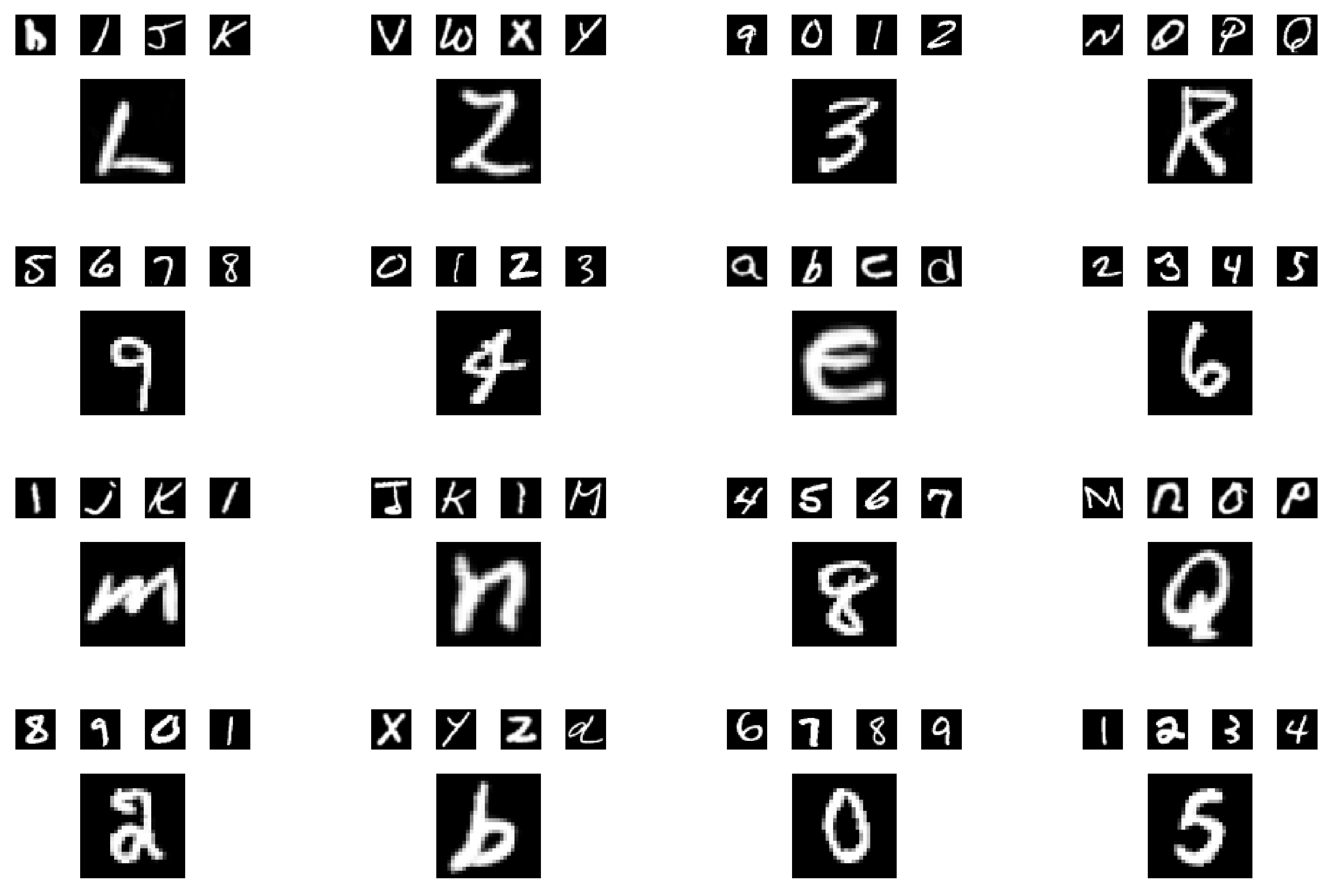
Indicative generative results during inference. In each case, the smaller upper symbols represent the input of the generator (unseen new data), while the larger single symbol below corresponds to the predicted outcome. For example, in the first case, we feed the generator with the letters (‘h’, ‘i’, ‘j’, ‘k’) and, as a result, we get the letter ‘l’ which is clearly correct.
Figure 7.
Indicative generative results during inference. In each case, the smaller upper symbols represent the input of the generator (unseen new data), while the larger single symbol below corresponds to the predicted outcome. For example, in the first case, we feed the generator with the letters (‘h’, ‘i’, ‘j’, ‘k’) and, as a result, we get the letter ‘l’ which is clearly correct.

Figure 8.
Illustrating the quality of two different chained predictions, at inference, for the digits’ dataset. In each case, the smaller upper digits represent the input of the generator, while the larger single digit corresponds to the predicted outcome. In the first link of each chain the input exclusively consists of samples originating from the test dataset. In the last link of each chain, the input exclusively consists of the samples that G generated in the previous links.

Figure 9.
Illustrating the quality of two different chained predictions, at inference, for the letters’ dataset. In each case, the smaller upper letters represent the input of the generator, while the larger single letter corresponds to the predicted outcome. In the first link of each chain the input exclusively consists of samples originating from the test dataset. In the last link of each chain the input exclusively consists of the samples that G generated in the previous links.

Figure 10.
A single-input chained prediction during inference. The generator receives an input image of the digit ‘7’ from the test set and correctly provides the next digit ‘8’ as his response. Subsequently, the resulting image of ‘8’ is fed back to G as a new input, predicting the digit ‘9’ as the next output and so on so forth.

Figure 11.
Characteristic examples of generated symbols (digits) during inference with the adoption of the Arbitrated Generative Adversarial Network (A-GAN) loss versus the utilization of the -GAN loss. In both cases, we contrast images from the highest performing models in terms of the derived accuracy.

Figure 12.
Characteristic examples of generated symbols (letters) during inference with the adoption of the A-GAN loss versus the utilization of the -GAN loss. In both cases, we contrast images from the highest performing models in terms of the derived accuracy.
Figure 12.
Characteristic examples of generated symbols (letters) during inference with the adoption of the A-GAN loss versus the utilization of the -GAN loss. In both cases, we contrast images from the highest performing models in terms of the derived accuracy.


Table 1.
Inference accuracy results in the chained prediction scenario for a highly capable model and, also, in a case where a considerable performance deterioration is observed from link to link. The results correspond to the digits’ dataset.
Table 1.
Inference accuracy results in the chained prediction scenario for a highly capable model and, also, in a case where a considerable performance deterioration is observed from link to link. The results correspond to the digits’ dataset.
| 1st in Chain | 2nd in Chain | 3rd in Chain | 4th in Chain | 5th in Chain | |
|---|---|---|---|---|---|
| Potent Model | 99.50% | 99.34% | 99.36% | 99.06% | 98.74% |
| Underperforming Model | 97.52% | 92.22% | 83.74% | 73.46% | 61.01% |
Table 2.
Inference accuracy results in the chained prediction scenario for a highly capable model and, also, in a case where a considerable performance deterioration is observed from link to link. The results correspond to the letters’ dataset.
Table 2.
Inference accuracy results in the chained prediction scenario for a highly capable model and, also, in a case where a considerable performance deterioration is observed from link to link. The results correspond to the letters’ dataset.
| 1st in Chain | 2nd in Chain | 3rd in Chain | 4th in Chain | 5th in Chain | |
|---|---|---|---|---|---|
| Potent Model | 95.84% | 94.88% | 93.08% | 92.36% | 91.28% |
| Underperforming Model | 88.18% | 85.90% | 80.08% | 72.29% | 60.71% |
Table 3.
Inference accuracy results in the chained prediction scenario for different cardinalities (value of t) of the training/testing input sequence. The results correspond to the digits’ dataset.
Table 3.
Inference accuracy results in the chained prediction scenario for different cardinalities (value of t) of the training/testing input sequence. The results correspond to the digits’ dataset.
| 1st in Chain | 2nd in Chain | 3rd in Chain | 4th in Chain | 5th in Chain | |
|---|---|---|---|---|---|
| 4 input frames | 99.50% | 99.34% | 99.36% | 99.06% | 98.74% |
| 3 input frames | 99.06% | 98.68% | 98.04% | 97.90% | 96.18% |
| 2 input frames | 98.08% | 97.46% | 96.86% | 95.46% | 92.92% |
| 1 input frame | 97.44% | 96.20% | 95.08% | 93.16% | 90.34% |
Table 4.
Inference accuracy results in the chained prediction scenario for different cardinalities (value of t) of the training/testing input sequence. The results correspond to the letters’ dataset.
Table 4.
Inference accuracy results in the chained prediction scenario for different cardinalities (value of t) of the training/testing input sequence. The results correspond to the letters’ dataset.
| 1st in Chain | 2nd in Chain | 3rd in Chain | 4th in Chain | 5th in Chain | |
|---|---|---|---|---|---|
| 4 input frames | 95.84% | 94.88% | 93.08% | 92.36% | 91.28% |
| 3 input frames | 94.54% | 92.82% | 91.45% | 89.72% | 87.13% |
| 2 input frames | 91.10% | 87.40% | 82.20% | 79.24% | 73.68% |
| 1 input frame | 85.50% | 76.12% | 67.24% | 60.62% | 54.02% |
Table 5.
Comparing the performance of various GAN models at inference, when using the arbiter’s classification loss versus the utilization of a pixel error-based loss, namely the loss. In bold, the best performing model of each corresponding comparison.
Table 5.
Comparing the performance of various GAN models at inference, when using the arbiter’s classification loss versus the utilization of a pixel error-based loss, namely the loss. In bold, the best performing model of each corresponding comparison.
| 1st in Chain | 2nd in Chain | 3rd in Chain | 4th in Chain | 5th in Chain | |
|---|---|---|---|---|---|
| A-GAN best case—digits | 99.50% | 99.34% | 99.36% | 99.06% | 98.74% |
| -GAN best case—digits | 99.26% | 99.34% | 99.20% | 99.04% | 98.71% |
| A-GAN best case—letters | 95.84% | 94.88% | 93.08% | 92.36% | 91.28% |
| -GAN best case—letters | 83.23% | 82.58% | 82.16% | 81.24% | 80.84% |
© 2020 by the authors. Licensee MDPI, Basel, Switzerland. This article is an open access article distributed under the terms and conditions of the Creative Commons Attribution (CC BY) license (http://creativecommons.org/licenses/by/4.0/).
Share and Cite
MDPI and ACS Style
Stivaktakis, R.; Tsagkatakis, G.; Tsakalides, P. Semantic Predictive Coding with Arbitrated Generative Adversarial Networks. Mach. Learn. Knowl. Extr. 2020, 2, 307-326. https://0-doi-org.brum.beds.ac.uk/10.3390/make2030017
AMA Style
Stivaktakis R, Tsagkatakis G, Tsakalides P. Semantic Predictive Coding with Arbitrated Generative Adversarial Networks. Machine Learning and Knowledge Extraction. 2020; 2(3):307-326. https://0-doi-org.brum.beds.ac.uk/10.3390/make2030017
Chicago/Turabian StyleStivaktakis, Radamanthys, Grigorios Tsagkatakis, and Panagiotis Tsakalides. 2020. "Semantic Predictive Coding with Arbitrated Generative Adversarial Networks" Machine Learning and Knowledge Extraction 2, no. 3: 307-326. https://0-doi-org.brum.beds.ac.uk/10.3390/make2030017