
Counterfactual Models for Fair and Adequate Explanations

1
Institut de Recherche en Informatique de Toulouse, Université Paul Sabatier, 31062 Toulouse, France
2
Institut de Mathématiques de Toulouse, Université Paul Sabatier, 31062 Toulouse, France
3
Telindus, 18 rue du Puits Romain, L-8070 Luxembourg, Luxembourg
4
Amazon Research, 72072 Tübingen, Germany
*
Author to whom correspondence should be addressed.
Mach. Learn. Knowl. Extr. 2022, 4(2), 316-349; https://0-doi-org.brum.beds.ac.uk/10.3390/make4020014
Submission received: 8 February 2022
/
Revised: 13 March 2022
/
Accepted: 15 March 2022
/
Published: 31 March 2022
(This article belongs to the Special Issue Selected Papers from CD-MAKE 2021 and ARES 2021)
Abstract
:Recent efforts have uncovered various methods for providing explanations that can help interpret the behavior of machine learning programs. Exact explanations with a rigorous logical foundation provide valid and complete explanations, but they have an epistemological problem: they are often too complex for humans to understand and too expensive to compute even with automated reasoning methods. Interpretability requires good explanations that humans can grasp and can compute. We take an important step toward specifying what good explanations are by analyzing the epistemically accessible and pragmatic aspects of explanations. We characterize sufficiently good, or fair and adequate, explanations in terms of counterfactuals and what we call the conundra of the explainee, the agent that requested the explanation. We provide a correspondence between logical and mathematical formulations for counterfactuals to examine the partiality of counterfactual explanations that can hide biases; we define fair and adequate explanations in such a setting. We provide formal results about the algorithmic complexity of fair and adequate explanations. We then detail two sophisticated counterfactual models, one based on causal graphs, and one based on transport theories. We show transport based models have several theoretical advantages over the competition as explanation frameworks for machine learning algorithms.
1. Introduction
Explaining the predictions of sophisticated machine-learning algorithms is an important issue for the foundations of AI. Recent efforts [1,2,3,4,5] have proposed various methods for providing explanations. Among these, model-based, logical approaches completely characterise one aspect of the decision offer complete and valid explanations. “Model-free” or model-agnostic, heuristic approaches like those in [1,2,6] cannot.
Model-based logical methods are thus a priori desirable, but they have an epistemological problem: they may be too complex for humans to understand or even to write down in human-readable form. Interpretability requires epistemically accessible explanations, explanations humans can grasp and compute. Yet what is a sufficiently complete and adequate epistemically accessible explanation, a good explanation still needs analysis [7].
We address this open question and characterize sufficiently good, or fair and adequate, explanations in terms of counterfactuals—explanations, that is that are framed in terms of what would have happened had certain conditions (that do not obtain) been the case. Counterfactual explanations, as we argue below, are a good place to start for finding accessible explanations, because they are typically more compact than other forms of explanation. While there have been many other counterfactual approaches, our approach is novel in that it provides an explicit, logical model for counterfactual explanations and links this model to techniques used to find counterfactual counterparts and explanations in ML systems like heat or saliency maps [8] or adversarial examples [3,9].
Another novel element of our approach is that for us a fair and adequate explanation must take into account the cognitive constraints and fairness requirements of an explainee [10,11,12]. asks for an explanation for why when she wasn’t expecting . Her not expecting follows from beliefs that must now be revised—how to specify this revision is the conundrum of . An adequate explanation is a pragmatic act that should solve the conundrum that gave rise to the request for explanation; solving the conundrum makes the explanation useful to [13]. In addition, an adequate explanation must lay bare biases that might be unfair or injurious to (the fairness constraint).
More precisely, we frame the pragmatic component of explanations in terms of what we call the conundrum and fairness requirements of the explainee, the person who requested the explanation or for whom the explanation is intended). It is this conundrum that makes the explainee request an explanation. This pragmatic act is naturally modelled in a game theoretic setting in which the explainer must understand explainee E’s conundrum and respond so as to resolve it. A cooperative explainer will provide an explanation in terms of the type he assigns to E, as the type will encode the relevant portions of E’s cognitive state. On the other hand the explainee will need to interpret the putative explanation in light of her model of the explainer’s view of his type. Thus, both explainer and explainee have strategies that exploit information about the other—naturally suggesting a game theoretic framework for analysis. Our theory thus analyzes the important pragmatic component of explanations and addresses a so far unsolved challenge for explanations noted by [14], according to which good, counterfactual explanations should take into account the explainee’s preferences and beliefs.
In an initial description of our view of fair and adequate explanations [15], we exploited both a logical theory of counterfactuals [16] and mathematical approaches for adversarial perturbation techniques [5,8,9,14,17,18,19,20,21] to prove a novel and precise correspondence between logical and mathematical formulations for counterfactuals. We then formalized conundra to provide a novel pragmatic notion of fair and adequate explanations, and we developed Explanation games for proving computational complexity results for finding fair and adequate explanations in non cooperative settings.
In this paper, we review some of the results of [15] in the first four sections. Section 2 provides a background to our view of explanations; Section 3 analyzes counterfactual explanations in more detail; Section 4 analyzes the pragmatic component of counterfactual explanations; and Section 5 analyzes the computational complexity of fair and adequate explanations. But in this paper, we have extended Section 3 to analyze the partiality of counterfactual explanations and how many other approaches that use counterfactual techniques often provide invalid explanations and hide possibly injurious biases. We have extended Section 5 to show how to use Explanation games to investigate properties of counterfactual models.
In addition, this paper has two sections with completely new work. In Section 6, we set out certain desiderata for counterfactual models that are more sophisticated than those in [15]. In Section 7, we propose two models of counterfactuals that are much more sophisticated than the ones contemplated in our earlier work—counterfactual models based on causal structural causal models or graphs, and counterfactual models based on transport theories. These models present much more sophisticated views of counterfactual counterparts. We extend our link between between logical and statistics based counterfactual methods to these sophisticated models. This leads us to change the underlying logical framework of counterfactuals by introducing probabilities explicitly into counterfactual semantics. We show that transport based approaches are especially interesting because they allow us to address in principle important challenges for applying counterfactual models to ML cited by [14]: first, transport methods allow us to construct counterfactual predictions based on partial data (when data about some features are missing). Second in some cases. they yield a set of counterfactuals that are equivalent to those provided by a causal theory. This means that we can have causally based counterfactuals in the absence of a fully specified causal structural model. A third advantage and potentially revolutionary advantage is that transport models form the basis of ML systems in which we can eliminate adversarial examples where the change in prediction of the system is not intelligible to examples in which the change in prediction is clearly intelligible and a classic case of a counterfactual counterpart [22].
As the reader will see, this is a theoretical paper. While we believe that experiments using various systems on different data sets can yield insights, we also think there is an important place for papers like this one that carve out a theoretical space. Our paper sets out a formal and explicit analysis of counterfactual explainability. We show how counterfactual models can address problems for ML systems at a theoretical level, and we address worst cases computational costs for fair and adequate explanations in some counterfactual models. In light of these developments, we think that the counterfactual approach has very rich empirical applications, some of which are explored in [22]; but adding a discussion of these applications would go far beyond this paper’s intended scope.
2. Background on Explanations
Following [10,11], we take explanations to be answers to why questions. Consider the case where a bank, perhaps using a machine learning program, judges ’s application for a bank loan and is turned down. is in a position to ask a why question like,
- (1)
- why was I turned down for a loan?
When her beliefs would not have predicted this. Her beliefs might not have been sufficient to infer that she wouldn’t get a loan; or her beliefs might have been mistaken—they might have led her to conclude that she would get the loan. In any case, must now revise her beliefs to accord with reality. Counterfactual explanations, explanations expressed with counterfactual statements, help do this by offering an incomplete list of relevant factors that together with unstated properties of entail the explanandum—the thing needs explained, in this case her not getting the loan. For instance, the bank might return the following answer to (1):
- (2)
- Your income is €50 K per year.
- (3)
- If your income had been €100 K per year, you would have gotten the loan.
The counterfactual statement (3) states what, given all of ’s other qualities, would have been sufficient to get the loan. But since her income is in fact not €100 K per year, the semantics of counterfactuals entails that does not get the loan. (3) also proposes to how to revise her beliefs to make them accord with reality, in that it suggests that she mistakenly thought that her actual salary was sufficient for getting the loan and that the correct salary level is €100 K per year. Ref. [23] provides a superficially similar picture to the pragmatic one we present, but their aim, to provide a semantics for argumentation frameworks, is quite different from ours. For us the pragmatic aspect of explanations is better explained via a game theoretic framework, as we shall see in Section 5.
Counterfactual explanations, we have seen, are partial, because they do not explicitly specify logically sufficient conditions for the prediction. They are also local, because their reliance on properties of a particular sample makes them valid typically only for that sample. Had we considered a different individual, say , the bank’s explanation for their treatment of might have differed. might have had different, relevant properties from ; for instance, might be just starting out on a promising career with a salary of €50 K per year, while is a retiree with a fixed income.
The partiality and locality of counterfactuals make them simpler and more epistemically accessible than other forms of model-based logical explanations. Logical methods often return rather long explanations even for relatively simple classifiers with large number of features that makes the explanations hard for humans to understand [24]. Nevertheless, the logical theory of counterfactuals enables us to move from a counterfactual to a complete and logically valid explanation. So in principle counterfactual explanations can provide both rigour and epistemic accessibility. But not just any partiality will do, since partiality makes possible explanations that are misleading, that hide injurious or unfair biases.
To show how the partiality of counterfactual explanations can hide unfair biases, consider the following scenario. The counterfactual in (2) might be true but it also might be misleading, hiding an unfair bias. (1) and (2) can be true while another, more morally repugnant explanation that hinges on ’s being female is also true. Had been male, she would have gotten the loan with her actual salary of €50 K per year. A fair and adequate explanation should expose such biases.
We now move to a more abstract setting. Let be a machine learning algorithm, with an n-dimensional feature space encoding data and Y the prediction space. Concretely, we assume that is some sort of classifier. When , an explainee may want an explanation, an answer to the question, “why ?” We will say that an explanation is an event by an explainer, the provider of the explanation, directed towards the explainee (the person requesting the explanation or to whom the explanation is directed) with a conundrum. An explanation will consist of of an explanandum, the event or prediction to be explained, an explanans, the information that is linked in some way to the explanandum so as to resolve the explainee’s conundrum. When the explanation is about a particular individual, we call that individual the focal point of the explanation.
Explanations have thus several parameters. The first is the scope of the explanation. For a global explanation of , the explainee wants to know the behavior of over the total space . But such an explanation may be practically uncomputable; and for many purposes, we might only want to know how behaves on a selection of data points of interest or focal points, like ’s bank profile in our example. Explanations that are restricted to focal points are local explanations.
Explanations of program behavior also differ as to the nature of the explanans. In this paper, we will be concerned with external explanations that involve an explanatory link between an explanans consisting of features of the input or feature space X, and the output in Y without considering any internal states of the learning mechanism [25]. These are attractive epistemically, because unpacking the algorithms’ internal states and assigning them a meaning can be a very complicated affair. Most explanations of complex ML systems like those that appeal to heat maps for instance are also external explanations. Most ML systems in effect are too complex or opaque for its behaviour to be analyzed statically.
Explanations are not only characterized by what sort of explanans they appeal to, a set of features in our case; they must also make explicit åhow the explanans is derived. To derive the explanans, we might have to appeal to the internal states of the learning mechanism. Explanations that use heat maps and gradient descent [8,26,27] do this as well as logic based explanations. These are all model = based types of explanation. On the other hand, explanations based on approximations of the behavior of the learning mechanisms like [1,2] do not use any internal states of the learning mechanism to find an explanans. The latter are known as model free explanations.
A third pertinent aspect of explanations concerns the link between explanans and the explanandum. Refs. [4,28,29] postulate a deductive or logical consequence link between explanans and explanandum. Ref. [4] represent as a set of logic formulas . By assuming features with finitely many values, an instance is then a set of literals that in which values are assigned to every feature in the feature space; if the features are binary, we can just have literals ℓ that such that ℓ represent the presence of a feature and the absence of that feature. An abductive explanation of why is a subset minimal set of literals such that . Abductive explanations exploit universal generalizations and a deductive consequence relation. They explain why any instance that has is such that and hence are known as global explanations [30]. On the other hand, model-free explanations typically don’t provide any explicit analysis of the relation between explanans and explanandum.
Counterfactuals offer a natural way to provide epistemically accessible, partial explanations of properties of individuals or focal points. The counterfactual in (3) gives a sufficient reason for ’s getting the loan, all other factors of her situation being equal or being as equal as possible (ceteris paribus) given the assumption of a different salary for . Such explanations are often called local explanations [30,31], as they depend on the nature of the focal point. Deductive explanations, on the other hand, are invariant with respect to the choice of focal point.
Counterfactual explanations are also partial [3], because the truth of the antecedent of a counterfactual is not by itself logically sufficient to yield the truth of the formula in the consequent. Model based counterfactual explanations instead derive logically sound predictions via points that verify the antecedent of the counterfactual and are minimally changed from the focal point. Because counterfactual explanations exploit ceteris paribus conditions, factors that deductive explanations must mention can remain implicit in a counterfactual explanation. Thus, counterfactual explanations are typically more compact and thus in principle easier to understand (see [29] for some experimental evidence of this). Counterfactuals are also intuitive vehicles for explanations as they also encode an analysis of causation [32].
Counterfactual Explanations for Learning Algorithms
A counterfactual language is a propositional language to which a two place modal operator is added. Its canonical semantics, as outlined in [16], for exploits a possible worlds model for propositional logic, , where: W is a non-empty set (of worlds), ≤ is a ternary similarity relation (), and assigns to elements in P, the set of proposition letters or atomic formulas of the logic, a function from worlds to truth values or set of possible worlds. Then, where ⊧ represents truth in such a model, we define truth recursively as usual for formulas of ordinary propositional logic and for counterfactuals , we have:
Definition 1.
just in case: .
What motivates this semantics with a similarity relation? We can find both epistemic and metaphysical motivations. Epistemically, finding a closest or most similar world in which the antecedent of the counterfactual is true to evaluate its consequent follows a principle of belief revision [33], according to which it is rational to make minimal revisions to one’s epistemic state upon acquiring new conflicting information. A metaphysical motivation comes from the link Lewis saw between counterfactuals and causation; implies that if hadn’t been the case, wouldn’t have been the case, capturing much of the semantics of the statement caused . The truth of such intuitive causal statements, however, relies on the presence of a host of secondary or enabling conditions. Intuitively the statement that if I had dropped this glass on the floor, it would have broken is true; but in order for the consequent to hold after dropping the glass, there are many elements that have to be the same in that counterfactual situation as in the actual world—the floor needs to be hard, there needs to be a gravitational field around the strength of the Earth’s that accelerates the glass towards the floor, and many other conditions. In other words, in order for such ordinary statements to be true, the situation in which one evaluates the consequent of a counterfactual has to resemble very closely the actual world.
Though intuitive, as this logical definition of counterfactuals stands, it is not immediately obvious how to apply it to explanations of learning algorithm behavior. We need to adapt it to a more analytical setting. We will do so by interpreting the similarity relation appealed to in the semantics of counterfactuals as a distance function or norm as in [34] over the feature space , an n-dimensional space, used to describe data points. To fill out our semantics for counterfactuals in this application, we identify instances in as the relevant “worlds” for the semantics of the counterfactuals.
We will fix a quantifier free counterfactual language with a finite set of variables for each dimension i of . To each and for each element in we will assign a value; in effect our elements in function like assignments. Our language will also contain a set of constants that designate values P that elements can take in . We add to this a set of formulas that describe the predictions in Y of . Atomic formulae are of the form and and the language is closed under Boolean operations and the counterfactual operator .
Notice that our learning function is itself not expressed in the language. Rather, it informs the counterfactual model as we see from the following definition. In addition our elements.
Definition 2.
A counterfactual model for with is a structure with D a non empty set containing , W a set of worlds , a norm on and , and .
We can now give the generic semantics for .
Definition 3.
Let be a counterfactual model for with .
- iff
- iff
- the usual clauses for and of
- just in case: if
Each instance in has a finite theory that is a conjunction of atomic formulae of the form where is a variable for dimension i and is its value. We now need to specify a norm for . A very simple norm assumes that each dimension of is orthogonal and has a Boolean set of values; in this case, has a natural norm or Manhattan or edit distance [35]. While this assumption commits us to the fact that the dimensions of capture all the causally relevant factors and that they are all independent—both of which are false for typical instances of learning algorithms, it is simple and makes our problem concrete. We will indicate below when our results depend on this simplifying assumption. Otherwise, we will only assume a finite set of finitely valued features through Section 5. In Section 6 and Section 7, we will complicate our language.
A logic of counterfactuals can now exploit the link between logic formulas, features of points in , and a learning algorithm described in [4,36,37]. Suppose a focal point is such that . A counterfactual that is true at the point , where is a prediction incompatible with , has an antecedent that is a conjunction of atomic formulae that defines a sufficient and minimal shift in the features of to get the prediction . Each counterfactual that explains the behavior of around a focal point thus defines a minimal transformation of the features of to change the prediction. This transformation can either be set valued or individual valued. Here we will consider them to be functions on for simplicity. We now define the transformations on that counterfactuals induce.
Definition 4.
Let be a set of variables designating values of dimensions I. A fixed transformation is a function such that for , if , then and differ only on values assigned to . We write to mean that and agree on the values assigned to . Given , and and where is a natural norm on , we shall be interested in the following types of transformations.
- (i)
- is appropriate if where η and π are two incompatible predictions in Y.
- (ii)
- is minimally appropriate if it is appropriate and in addition, such that and , .
- (iii)
- is sufficiently appropriate if it is appropriate and in addition, for any , is not appropriate.
- (iv)
- is sufficiently minimally appropriate if it is both sufficiently and minimally appropriate.
Note that when X is a space of Boolean features, then conditions (ii) and (iv) of Definition 4 trivially hold. Given a focal point in , minimally appropriate transformations represent the minimal changes necessary to the features of to bring about a change in the value predicted by .
Let and consider now a counterfactual language . Given a counterfactual model for with norm on , we say that is definable just in case for any worlds there is a formula of , which we call a separating formula, such that for all , and .
Proposition 1.
Let and let be a counterfactual model for with an definable norm. Suppose also that . Then:
, where and ϕ is a separating formula that assigns values to variables for iff there is a minimally appropriate transformation such that , and .
Proposition 1 follows easily from Definitions 1, 2 and 4.
Proposition 1 is general and can apply to many different norms and languages. We will sometimes be concerned here with a special and simple case:
Corollary 1.
Let be a propositional counterfactual language with a set P of propositional letters, where P is the set of Boolean valued features of , and let be a counterfactual model for with an norm. Then: , where and ψ is a conjunction of literals in P iff there is a minimally appropriate transformation over the dimensions I fixed by ψ such that , and .
We can generate minimally appropriate transformations via efficient (poly-time) techniques like optimal transport or diffeomorphic deformations [5,17,18,19,20,21] or techniques for computing adversarial perturbations [9]. In effect all of these diverse methods yield counterfactuals or sets of counterfactuals given Proposition 1. A typical definition of an adversarial perturbation of an instance x, given a classifier, is that it is a smallest change to x such that the classification changes. Essentially, this is a counterfactual by a different name. Finding a closest possible world to x such that the classification changes is, under the right choice of distance function, the same as finding the smallest change to x to get the classifier to make a different prediction. Such minimal perturbations may not reflect the ground truth, the causal facts that our machine learning algorithm is supposed to capture with its predictions, as noted by [38]. We deal with this in Section 3.
Proposition 1 has two advantages. First it offers, as we shall see later, a way to define various counterfactual models defined with increasingly sophisticated transformations. Second, it marries efficient techniques to generate counterfactual explanations with the logical semantics of counterfactuals that provides logically valid (LV) explanations from counterfactual explanations, unlike heuristic, model-free methods [2,39]. Thus, counterfactual explanations build a bridge between logical rigor and computational feasibility.
Proposition 2.
A counterfactual explanation given by a minimally appropriate in , with an definable norm and with finitely many values for each yields a minimal, LV explanation in at worst a linear number of calls to an NP oracle.
Proof sketch.
Recall that each “world” or point of evaluation is encoded as a conjunction of literals for some values (the variables representing features or dimensions of ). Together with the logical representation of , this suffices to reconstruct the atomic diagram of [40]. Further, given Corollary 1 and Definition 2, each minimally appropriate defines a set of literals describing such that . Refs. [4,29] provide an algorithm for finding a subset minimal set of literals with in a linear number relative to of calls to an NP oracle [41]. □
3. From Partial to More Complete Explanations
We have observed that counterfactual explanations are intuitively simpler than deductive ones, as they typically offer only a partial explanation. In fact there are three sorts of partiality in a counterfactual explanation. First, a counterfactual explanation is deductively incomplete; it doesn’t specify the ceteris paribus conditions and so doesn’t specify what is necessary for a proof of the prediction for a particular focal point. Second, counterfactual explanations are also partial in the sense that they don’t specify all the sufficient conditions that lead to ; they are hence globally incomplete. Finally, counterfactuals are partial in a third sense; they are also locally incomplete. To explain this sense, we need the notion of overdetermination.
Definition 5.
A prediction by is overdetermined for a focal point if the set of minimally sufficiently appropriate transformations of
contains at least two elements.
Locally incomplete explanations via counterfactuals can occur whenever ’s counterfactual decisions are over-determined for a given focal point. Many real world applications like our bank loan example will have this feature.
These different forms of partiality affect many heuristic forms of explanation and can lead to bad explanations or interpretations of ML systems. Refs. [24,42] show that heuristic counterfactual models like those proposed by [1,2,6] often give unsound explanations for a classifier’s predictions. Moreover, heuristic approaches to explanation like Lime, Anchor and Shap provide explanations unmoored from their underpinnings in counterfactual semantics. Thus, the explanations they provide are naturally understood as simple premises of a deductive explanation The problem is, for such approaches we can find two focal points and such that the approaches return the same explanans for the predictions and but and are incompatible. And this is unsound: in a sound explanation cannot serve as an explanans in a deductive explanation to both and .
Given our framework, it is not hard to see why these heuristic frameworks do this; they are in fact offering counterfactual explanations but without taking into account or making explicit the fact that counterfactual explanations assume that certain ceteris paribus conditions are assumed to hold. These ceteris paribus conditions make counterfactual explanations deductively incomplete, and so when using explanations to verify or to interpret a ML algorithm’s behavior, we have to take this partiality into account. Worse, these systems are sometimes interpreted as providing globally valid explanations, which ignores the second kind of incompleteness of counterfactual explanations. In the current framework on the other hand, Proposition 2 shows exactly how to get a deductively valid, global explanation from a counterfactual one, something which heuristic approaches to counterfactual explanations are not able to do.
Finally, locally incomplete explanations can, given a particular ML model , hide implicitly defined properties that show to be unacceptably biased in some way and so pose a problem for fair and adequate explanations. Local incompleteness allows for several explanatory counterfactuals with very different explanans to be simultaneously true. This means that even with an explanation, may act in ways unknown to the agent or the public that is biased or unfair. Worse, the constructor or owner of will be able to conceal this fact if the decision for is overdetermined, by offering counterfactual explanations using maps that don’t mention the biased feature.
Definition 6.
A prejudicial factor P is a map, and exhibits a biased dependency on prejudicial factor P just in case for some , , and for some incompatible predictions η and π,
Dimensions of the feature space that are atomic formulas in can provide examples of a prejudicial factor P. But prejudical factors P may be also implicitly definable in a counterfactual model . Assume that is a map from real individuals x to their representation as data points . Recall that each point is uniquely identified by a formula for some values . Then:
Definition 7.
Some exogenous property P is implicitly definable just in case for all x such that , iff for some boolean combination of atomic formulas, χ, .
All in all, our analysis shows why forms of counterfactual explanations that do not take into account the logical underpinnings of a counterfactual framework will give flawed results.
We’ve just described some pitfalls of locally incomplete counterfactual explanations. Thanks to Proposition 1, however, our logic based and statistical counterfactual framework shows how to move from a partial picture of the behavior of to a more complete one using counterfactuals. Again this is a feature that heuristic approaches but also deductive logical approaches do not have. Imagine that at a focal point , and we want to know why not .
Definition 8.
In a counterfactual model with a set of Boolean valued features P, the collection of counterfactuals with ϕ a Boolean combination of values for atoms in true at gives the complete explanation for why π would have occurred at .
Appropriate transformations on in a counterfactual model to produce associated with counterfactuals via Proposition 1 can capture and permit us to plot the local complete explanation of around a focal point with regard to prediction .
Definition 9.
is a minimal appropriate transformation for some
Proposition 3.
In a counterfactual model ,
We now fix a counterfactual model to simplify notation.
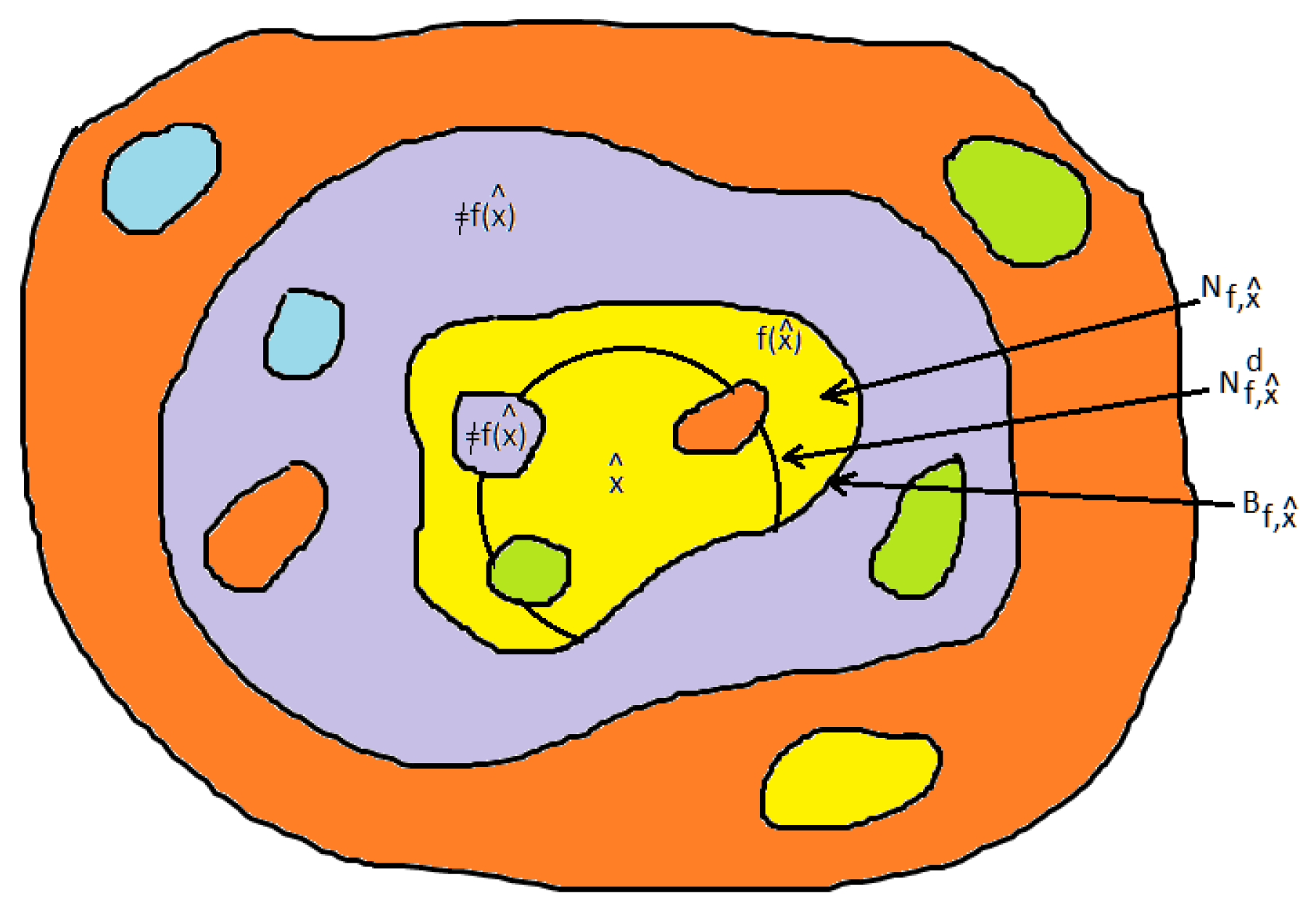
We are interested in the neighborhood or “similarity” space around with boundary and the targeted outcome space verifying the consequent of counterfactuals in .
Definition 10.
- 1.
- is the subspace of such that (i) and (ii) includes in its interior all those points z for which and (iii) the boundary of is given by .
- 2.
- is a subspace of with boundary , where , where
- 3.
The set can have a complex or “gappy” structure in virtue of the presence of ceteris paribus assumptions. Because strengthening of the antecedent fails in semantics for counterfactuals, the counterfactuals in (4) relevant to our example of Section 2 are all satisfiable at a world without forcing the antecedents of (4)b or (4)c to be inconsistent:
- (4)
- a.
- If I were making €100 K euro, I would have gotten the loan.
- b.
- If I were making €100 K or more but were convicted of a serious financial fraud, I would not get the loan.
- c.
- If I were making €100 K or more and were convicted of a serious financial fraud but then the conviction was overturned and I was awarded a medal, I would get the loan.
The closest worlds in which I make €100 K do not include a world w in which I make €100 K but am also convicted of fraud. Counterfactuals share this property with other conditionals that have been studied in nonmonotonic reasoning [43,44]. However, if the actual world turns out to be like w, then by weak centering (4)a turns out to be false, because the ceteris paribus assumption in (4)a is that the actual world is one in which I’m not convicted of fraud.
Figure 1 provides a visual rendering of (in purple) and related concepts.
Given we can count how many times the value of the consequent changes of flips as we move from one antecedent to a logically more specific one; e.g., does the prediction flip from A to or from to ? For generality, we will also include in the number of flips, the flips that happen when we change the Boolean value of a feature—going from A to for example. We will call the number of flips the flip degree of , as well as of .
There is an important connection between the flip degree of and the geometry of . In a counterfactual model, the move from one antecedent of a counterfactual a to logically more specific antecedent of , with will, given certain assumptions about the underlying norm yield , with y being a closest to point verifying and z a closest point verifying . In fact we generalize this property of norms.
Definition 11.
A norm in a counterfactual model respects the logical specificity of the model iff for any such that and for counterfactual antecedents describing features of such that such that and , there are collinear such that for each i, is a closest point to z such that and .
Remark 1.
An L1 norm for a counterfactual model is a logical specificity respecting norm.
In addition, a flip (move from a point verifying to a point verifying corresponds to a move from a transformation to a transformation with . Thus, flips determine a partial ordering under ⊆ over the shifted dimensions i: thus , if . We are interested in the behavior of with respect to the partial ordering on .
Definition 12.
is nearly constant around , if for every sufficiently minimally appropriate for all , .
A nearly constant changes values only once for each combination of features/dimensions moving out from a focal point . So at some distance d, nearly constant becomes constant . For a nearly constant around , , has flip degree 1. A complete local explanation for ’s prediction of within d, , is a global explanation ’s behavior with respect to .
We can generalize this notion to define an n-shifting . If flips values n times moving out from , has flip degree n.
Remark 2.
If , has flip degree 1, then a counterfactual explanation of ’s behavior with respect to π is also a formally valid, abductive explanation.
Corollary 2.
Let be any ML algorithm that is nearly constant around and with an associated for which there is a polynomial procedure for finding a suitable minimal . Then we can find an abductive explanation for ’s behavior at in polynomial time.
Proposition 4.
Suppose A counterfactual model has a logical specificity respecting norm, then: , has a flip degree iff forms a convex subspace of .
Proof sketch.
Assume has flip degree . Then will contain counterfactuals with antecedents , , such that but, say, and counterfactually support but not . As the underlying norm respects ⊧, there are collinear points x, y, and z, where x is a closest point to where is true, y is a closest world, and z is a closest world such that . But , while and , which makes non convex. Conversely, suppose is non convex. Using the construction of counterfactuals from the boundary of will yield a set with flip degree 3 or higher. □
The flip degree of gives a measure of the degree of non-convexity of , and a measure of the complexity of an explanation of ’s behavior. A low flip degree for with minimal overdeterminations provides a more general and comprehensive explanation. With Proposition 4, a low flip degree converts a local complete explanation into a global explanation, which is a priori preferable. It is also arguably closer to our prior beliefs about basic causal processes. The size of gives us a measure to evaluate itself; a large doesn’t approximate very well a good scientific theory or the causal structures postulated by science. Such a lacks generality; it has neither captured the sufficient nor the necessary conditions for its predictions in a clear way. This could be due to a bad choice of features determining ’s input [20]; too low level or unintuitive features could lead to lack of generality with high flip degrees and numerous overdeterminations. Thus, we can use to evaluate and its input representation .
Can we exploit flip degrees to have bounds on the confidence of our explanations? Yes, perhaps we can. Let us suppose that exogenously given to us is a probability distribution over the features of samples in . We could calculate this distribution relative to itself. Let us suppose we have calculated joint probability distributions for all of the antecedents of conditionals in , where is the antecedent for the counterfactual that gives flip number i.
Proposition 5.
Suppose that the flip degree of but that , for . Then that furnishes a formally valid, abductive explanation.
The flip degree of and the topology of can also tell us about the relation between counterfactual explanations based on some element in X and ground truth instances provided during training. Our learning algorithm is trying to approximate or learn some phenomenon, which we can represent as a function ; the observed pairs are ground truth points for . Ideally, should fit and converge to f—i.e., with the number of data points N is trained on ; in the limit explanations of the behavior of will explain f, the phenomenon we want to understand. Given that we generate counterfactual situations using techniques used to find adversarial examples, however, counterfactual explanations may also be based on adversarial examples that have little to no intuitive connection with the ground truth instances was trained on. While these can serve to explain the behavior of and as such can be valuable, they typically aren’t good explanations of the phenomenon f that is trying to model. Ref. [38] seek to isolate good explanations of f from the behavior of and propose a criterion of topological connectedness for good counterfactual explanations. This idea readily be implemented as a constraint on : roughly, as an approximation of f will yield good counterfactual explanations relative to a focal point only if for any point y outside of , there is a region C where returns the same value and a path of points between y and a ground truth data point p such that . (We note that our discussion and constraint make clear the distinction between f and which is implicit in [13,38]).
4. Pragmatic Constraints on Explanations
While we have clarified the partiality of counterfactual explanations, AI applications can encode data via hundreds even thousands of features. Even for our simple running example of a bank loan program, the number of parameters might provide a substantial set of counterfactuals in the complete local explanation given by . This complete local explanation might very well involve too many counterfactuals for humans to grasp. We still to understand what counterfactual explanations are pragmatically relevant in a given case.
Pragmatic relevance relies on two observations. First, once we move out a certain distance from the focal point, then the counterfactual shifts intuitively cease to be about the focal point; they cease to be counterparts of and become a different case. Exactly what that distance is, however, will depend on a variety of factors about the explainee and what the explainer believes about . Second, appropriate explanations must respond to the particular conundrum or cognitive problem that led to ask for the explanation [10,11,12]. On our view, the explainee requires an explanation when her beliefs do not lead her to expect the observed prediction . When ’s beliefs suffice to predict , she has a priori an answer to the question Why did ? In our bank example from Section 2, had ’s beliefs been such that she did not expect a loan from the bank, she wouldn’t have needed to ask, why did the bank not give me a loan? Of course, might want to know whether her beliefs matched the bank’s reasons for denying her a loan, but that’s a different question—and in particular it’s not a why question).
The conundrum comes from a mismatch between ’s understanding of what was supposed to model (our function f) and ’s actual predictions. So , in requesting an explanation of ’s behavior, might also want an explanation of f itself (see the previous section for a discussion). Either is mistaken about the nature of , or her grasp of is incomplete ( could also be mistaken about or have an incomplete grasp of f; she might also be mistaken about how differs from f. But we will not pursue this here). More often than not, will have certain preconceptions about , and then many if not most of the counterfactuals in may be irrelevant to . A relevant or fair and adequate explanation for should provide a set of appropriate with showing which of ’s assumptions were faulty or incomplete, thus solving her conundrum.
Suppose that the explainee requests an explanation why , and that is decomposed into .
- CI
- Suppose ’s conundrum based on incompleteness; i.e., the conundrum arises from the fact that for only pays attention to the values of dimensions in the sense that for her , for any values . Then there is a such that and while
- CM
- Suppose ’s conundrum is based on a mistake. Then there is a such that such that . I.e., must resolve ’s conundrum by providing the values for the dimensions of on which is mistaken.
A fair and adequate explanation must not only contain counterfactuals that resolve the explainee’s conundrum. It must make clear the biases of the system which may account for 0’s incomplete understanding of ; it must lay bare any prejudicial factors P that affect the explainee and thus in effect all overdetermining factors as in Definition 5. An explainee might reasonably want to know whether such biases resulted in a prediction concerning her. E.g., the explanation in (3) might satisfy CM or CI, but still be misleading. Thus:
- CB
- ∀ prejudicial factors P, there is a such that and . In our bank loan example, if the bank is constrained to provide an explanation obeying CB, then it must provide an explanation according to which being white and having ’s salary would have sufficed to get the loan.
Definition 13.
A set of counterfactuals provides a fair and adequate explanation of for at just in case they together satisfy CM, CI and CB within a certain distance d of .
The counterfactuals in jointly provide a fair and adequate explanation of for , though individually they may not satisfy all of the constraints. We investigate how hard it is to find an adequate local explanation in the next section.
5. The Algorithmic Complexity of Finding Fair and Adequate Explanations
In this section, we examine the computational complexity of finding a fair and adequate explanation. To find an appropriate explanation, we imagine a game played, say, between the bank and the would-be loan taker in our example from Section 2, in which can ask questions of the bank (or owner/developer of the algorithm) about the algorithm’s decisions. We propose to use a two player game, an explanation game to get appropriate explanations for the explainee.
The pragmatic nature of explanations already motivates the use of a game theoretic framework. We have argued fair and adequate explanations must obey pragmatic constraints; and in order to satisfy these in a cooperative game the explainer must understand explainee ’s conundrum and respond so as to resolve it. Providing an explanation is a pragmatic act that takes into account an explainee’s cognitive state and the conundrum it engenders for the particular fact that needs explaining. A cooperative explainer will provide an explanation in terms of the type he assigns to , as the type will encode the relevant portions of ’s cognitive state. On the other hand the explainee will need to interpret the putative explanation in light of her model of the explainer’s view of his type. Thus, both explainer and explainee naturally have strategies that exploit information about the other. Signaling games [45] are a well-understood and natural formal framework in which to explore the interactions between explainer and explainee; the game theoretic machinery we develop below can be easily adapted into a signaling game between explainer and explainee where explanations succeed when their strategies coordinate on the same outcome.
Rather than develop signaling games however for coordinating on successful explanations, we look at non-cooperative scenarios where the explainer may attempt to hide a good explanation. For instance, the bank in our running example might have encoded directly or indirectly biases into its loan program that are prejudicial to , and it might not want to expose these biases. The games below provide a formal account of the difficulty our explainee has in finding a winning strategy in such a setting.
To define an explanation game, we first fix a set of two players .
The moves or actions for explainee are: playing an ACCEPT move—in which accepts a proposed if it partially solves her conundrum; playing an N-REQUEST move—i.e., requesting a where j differs from all i such that has been proposed by in prior play; playing a P-REQUEST move—i.e., for some particular i, requesting . may also play a CHALLENGE move, in which claims that a set of features of the focal point that entails in the counterfactual model associated with . We distinguish three types of ME explanation games for based on the types of moves she is allowed: the Forcing ME explanation games, in which may play ACCEPT, N-REQUEST, P-REQUEST; the more restrictive Restriction ME explanation games, in which may only play ACCEPT, N-REQUEST; and finally Challenge ME explanation games in which CHALLENGE moves are allowed.
Adversary ’s moves consists of the following: producing and computing in response to N-REQUEST or P-REQUEST by ; if is a forcing game, must play at move m in , if has played P-REQUEST at . In reacting to a N-REQUEST, player may offer any new ; if he is noncooperative, he will offer a new that is not relevant to ’s conundrum, unless he has no other choice. On the other hand, must react to a CHALLENGE move by by playing a that either completes or corrects the Challenge assumption. A CHALLENGE demands a cooperative response; and since it can involve any implicitly definable prejudicial factor as in Definition 5, it can also establish CB, as well as remedy CI or CM.
5.1. Generic Explanation Games
We now specify a win-lose, generic explanation game.
Definition 14.
An Explanation game , , concerning a polynomially computable function , where is a space of boolean valued features for the data and Y a set of predictions, is a tuple where:
- i.
- resolves ’s conundrum and obeys CB.
- ii.
- is the starting position, d is the antecedently fixed distance parameter.
- iii.
- , but not has access to the behavior of and a fortiori .
- iv.
- opens with a REQUEST or CHALLENGE move
- v.
- responds to ’s requests by playing some .
- vi.
- may either play ACCEPT, in which case the game ends or again play a REQUEST or CHALLENGE move.
- vii.
- is the set of plays ρ that contain the sufficient to resolve (resolve ’s conundra)
The game terminates when (a) has resolved or gives up.
always has a winning strategy in an explanation game. The real question is how quickly can compute her winning condition. An answer depends on what moves we allow for in the Explanation game; we can restrict to playing a Restriction explanation game, a Forcing game or a Forcing game with CHALLENGE moves.
Proposition 6.
Proof sketch.
Finding is a search problem using . is finite with, say, m elements. These elements need not be unique; they just need jointly to solve the conundrum. This search problem is PLS just in case every solution element is polynomially bounded in the size of the input instance, is poly-time, the cost of the solution is poly-time and it is possible to find the neighbors of any solution in poly-time. Let be the input instance. By assumption, is polynomial; and given the bound d, the solutions y for and are polynomially bounded in the size of the description of . Now, finding a point that solves at least part of ’s conundrum, as well as finding neighbors of y is poly-time, since can use P-REQUEST moves to direct the search. To determine the cost c of finding for in poly-time: we set for the jth element of computed as ; if , . Finding thus involves determining m local minima and is PLS. In addition, determining encodes the PLS complete problem FLIP [46]: the solutions y in have the same edit distance as the solutions in FLIP, encodes a starting position, and our cost function can be recoded over the values of the Boolean features defining y to encode the cost function of FLIP and the function that compares solutions in FLIP is also needed and constructible in . So finding is PLS complete in as it encodes FLIP.
The fact that forcing explanation games are PLS complete makes getting an appropriate explanation computationally difficult. Worse, if is a Restriction Explanation game, then can force to enumerate all possible within radius d of to find . □
Proposition 7.
Suppose is a Challenge explanation game. Then has a winning strategy in that is linear time computable, provided ’s values are already known.
Proof sketch.
must respond to ’s CHALLENGE moves by correcting or completing ’s proposed list of features. can determine in a number of moves that is linear in the size of . □
A Challenge explanation game mimics a coordination game where has perfect information about , because it forces cooperativity and coordination on the part of . Suppose in our bank example claims that her salary should be sufficient for a loan. In response to the challenge, the bank could claim the salary is not sufficient; but that’s not true—the salary is sufficient provided other conditions hold. That is, ’s conundrum is an instance of CI. Because of the constraint on CHALLENGE answers by the opponent, the bank must complete the missing element: if you were white with a salary of €50 K, … Proposition 7 shows that when investigating an in a challenge game, exploiting a conundrum is a highly efficient strategy. Of course we’re here not counting the fact that computing takes polynomial time since we have assumed that computing is poly time.
The flip degree of and the number of overdetermining factors (Definition 5) typically affect the size of and thus the complexity of the conundrum and search for fair and adequate explanations and their logical valid associates. More particularly, when and the cost of the prediction is as in the proof of Proposition 6, ’s conundrum and the explanations resolving it may require n local minima. When the flip degree of is m, may need to compute m local minima.
To develop practical algorithms for fair and adequate explanations for AI systems, we need to isolate ’s conundrum. This will enable us to exploit the efficiencies of Challenge explanation games. Extending the framework to discover ’s conundrum behind her request for an explanation is something we plan to do using epistemic games from [48] with more developed linguistic moves. In a more restricted setting where Challenge games are not available, our game framework shows that clever search algorithms and heuristics for PLS problems will be essential to providing users with relevant, and provably fair and adequate counterfactual explanations. This is something current techniques like enumeration or finding closest counterparts, which may not be relevant [4,29,37]—do not do.
5.2. Exploring Counterfactual Models with Explanation Games
Explanation games can be used also to discover facts about and about the explanatory generalizability of an explanation for a prediction of at a particular focal point. For instance, a Forcing game can be used to establish a degree of robustness of around a focal point, in the sense that we can compute a radius d and a ball around such that . In such a case we can say that has a local Lipschitz robustness of degree 0 in a ball of radius d around , since for any points in . By calculating d, we can establish the robustness also of our counterfactual explanation at in the sense of [49]. The techniques used Proposition 6 can also be used to establish the extent of . In addition, techniques to generate adversarial examples can help us determine perhaps more efficiently the radius of .
Another use for the sort of games we have introduced in this section is to find confounders. Consider our loan example in which is robust with respect to changes on a particular variable for race ( if is a disfavored minority and is 1 otherwise); that is, where and differ only on values for dimension i. But in fact varies on variables for diet ( if diet is that of a disfavored minority) and home address ( if home address is in an affluent neighborhood, 0 otherwise). It turns out that there is a very strong correlation between and ; an overwhelming number of disfavored minority class members represented in are such that their theories entail . While the bank might claim that its algorithm is racially insensitive by cherry-picking certain cases—namely those individuals y for which their theories are such that and , in either a Challenge or forcing Explanation game will be able to establish an implicit and unfair bias in by continuing to ask for predictions on individuals for whom . This is even possible if race is not explicitly represented as a dimension in , as long as it is implicitly definable in the model. Note that this procedure to find confounders is also useful for showing whether is biased for or against a particular group.
To formalize this search for confounders, we tweak the notion of an explanation game to define an explanation investigation game. We do not need to rely on Boolean features for the data; they can even be continuously valued.
Definition 15.
An explanation investigation game , , concerning a polynomially computable function , is a tuple where:
- i.
- Suppose for some values , implicitly defines in a subset P of individuals where .
- ii.
- has access to the implicit definition of ϕ in
- iii.
- , but not has access to the behavior of .
- iv.
- wins if she discovers a pair in (i); i.e., a play iff it ends with an for some such that where and .
- v.
- opens with a REQUEST move concerning some
- vi.
- responds to ’s requests by playing some that applies to .
Remark 3.
Let be a forcing explanation investigation game where for and . Then has a winning strategy in in polynomial time.
We can strengthen Remark 3 by considering a stronger winning condition: suppose P is finite and is to find a sufficiently large sample of pairs. In this case, if the assumptions of Remark 3 are met, also has a winning strategy in with calls to . If is large or if is not sufficiently representative, then this strategy may not be feasible to establish the presence of confounders or their absence. We need more information from the counterfactual model to do this. In Section 7, we will see an example of a counterfactual model that can help us.
More generally, a forcing explanation investigation game can detect dependencies between features that may have gone unnoticed by the designers of . Just as we can find implicit equivalences between Boolean combinations of feature value assignments and other properties, so too will an explanation investigation game be able to detect equivalences between two Boolean combinations of feature value assignments, incompatibilities or independence. We can establish these relations either relative to some finite set or globally relative to all points in by moving from the counterfactual model to the proof theory that encodes and the input data.
6. Generalizing towards More Sophisticated Counterfactual Models
While much of our exploration has been general, some results, in particular those of the previous section, have relied on a particularly simple notion of norm or distance to define counterfactual counterparts. In the remainder of the paper, we want to look at other ways of defining more sophisticated counterfactual models. We look at three different ways to generalize the simple models above: generalizing from very simple norms, adding indeterminism, adding randomness, and providing counterfactual correlates that take account of dependencies and distributions. We then look at two types of counterfactual models, one based on causal graphs and another based on transport theories. We argue that transport based counterfactual models should provide very relevant explanations of an algorithm’s behavior.
6.1. Moving from an L1 Norm to More Sophisticated Ways of Determining Counterfactual Correlates
Specifying a norm for our space of data is crucial for building a counterfactual model and specifying counterfactual correlates. But when we have specified a norm, it has been a very simple one that assumes that each dimension of is orthogonal and has a Boolean set of values; in this case, has a natural norm or Manhattan or edit distance [35]. But for this choice of norm to make sense we must assume that the dimensions of are all independent, and this assumption is not only manifestly false for typical instances of learning algorithms but also gives very unintuitive results in concrete cases [50].
For example, consider a set of data with dimensions for sex, weight and height; and now consider the counterfactual assumption Nicholas is a woman. Assume that Nicholas is slightly over average in weight and about average in height for men. But now consider his counterfactual counterfactual female counterpart with the same weight and height as the actual Nicholas. This counterpart would be an outlier in the distribution of females over those dimensions, thus making the following counterfactual true. ex. If Nicholas were a woman, she would be unusually heavy and unusually tall.
Intuitions differ here, but most people find such counterfactuals rather odd, if not false. Much more acceptable would be a counterfactual where we explicitly restrict the counterfactual counterpart to have exactly all of Nicholas’s current properties. ex. If Nicholas were a woman and she had the same height and weight as Nicholas actually does, she would be unusually heavy and unusually tall.
If one shares these intuitions, then it appears that we need to reframe a counterfactual model in terms of a more sophisticated notion of counterfactual correlate. What we want is a notion of counterfactual correlate where the dependencies between features are taken into account.
6.2. Adding Indeterminism
Given Proposition 1, we can rewrite a counterfactual model in terms of a set of minimal appropriate transformations and exploit this in the semantics of counterfactuals:
Definition 16.
Counterfactual semantics with transformations:
be a counterfactual model with transformations that extends a standard counterfactual model for with with a set of minimal adequate transformations for each set of variables .
Let ψ define a set of values for variables . Then just in case:
The transformations now define the relevant counterfactual counterparts directly for the semantics. Note that each standard counterfactual model obviously extends to a counterfactual model with transformations in view of Proposition 1.
Another restriction in the work in the previous sections is that our transformations so far have been single valued functions. That is, if any element in xX has a counterfactual element, it is unique. This forces our models to verify conditional excluded middle, which could be unintuitive.
Definition 17.
Conditional Excluded Middle:
Consider, for example, the intervention on my salary where I make €100 K per year instead of €60 K. Such an intervention does not determine all of my properties. In a counterfactual situation where I make €100 K instead of €60 K, I might still have the same bicycle that I go to work on. Or I might not. There doesn’t seem to be a set answer to the question,
- (5)
- Were Nicholas to make €100 K per year, would he still use the same bicycle he does now to go to work?
But with conditional excluded middle, a counterfactual model must support one of
- (6)
- (a.)
- Were Nicholas to make €100 K per year, he would use the same bicycle he does now to go to work.
- (b.)
- Were Nicholas to make €100 K per year, he not would use the same bicycle he does now to go to work.
A counterfactual asks us to entertain a situtation different from the current one. In semantic terms, the antecedent of a counterfactual introduces an “intervention” into the actual circumstance of evaluation that shifts us away from that circumstance to a different one in which the antecedent is true, thereby defining a counterfactual correlate. Our argument of the previous paragraph indicates that such an intervention does not determine every property of the correlate.
We can remedy this defect of our semantics by lifting our transformations to set valued functions. i.e.,
Definition 18.
Let . A set valued fixed transformation is a function , where is the powerset operation, such that for and , if , then x and y differ in the dimensions i. Given , and and where is a natural norm on ,
- (i)
- is appropriate if with and π incompatible predictions in Y.
- (ii)
- is minimally appropriate if it is appropriate and,and , .
With set valued transformations, we can build counterfactual models as before. The difference now is that conditional excluded middle is no longer valid.
Definition 19.
Let ψ define a set of values for a set of variables and let be a counterfactual model with a set D of minimal appropriate set valued transformations . just in case:
6.3. Introducing Randomness and Probabilities
Using set valued transformations has introduced indeterminism into our counterfactual models. With indeterminism, not every intervention described by the antecedent of a counterfactual yields a unique outcome. In fact, this sort of indeterminism is a feature of Lewisian counterfactuals [16], where counterfactual correlates may or may not have certain properties. Once such indeterminism is introduced, however, it is also natural to take the counterfactual correlates as more or less likely to have those properties. That is, it is natural to add to our indeterministic picture a notion of probability, a probability distribution over the properties that counterfactual correlates may exhibit.
Consider again the intervention on my salary where I make €100 K instead of €60 K euros. Such an intervention we’ve argued does not determine all of my properties. In a counterfactual situation where I make €100 K instead of €60 K, I might still have the same bicycle that I go to work on. Or I might not. That is, the counterfactuals in (6) repeated below are plausibly both false.
- (7)
- a.
- Were Nicholas to make €100 K euros per year, he would use the same bicycle he does now to go to work.
- b.
- Were Nicholas to make €100 K euros per year, he not would use the same bicycle he does now to go to work.
On the other hand, a probabilistic statement like
- (8)
- Were Nicholas to make €100 K euros per year, there is a 70% chance that he would use the same bicycle he does now to go to work.
is plausible. We find this addition to the semantics of counterfactuals very appealing. Adding probabilities to the logic of counterfactuals, however, takes us far beyond the framework of Lewis’s semantics for counterfactuals. Ref. [51] argues that a logical semantics for languages with probabilities comes in two types, because probabilities can be used to represent two different kinds of information as [51,52,53] have argued. One sort of information has to do with degrees of belief; that is, to what degree, for instance, does Nicholas believe that he will use his bicycle to go to work? We can represent following [53] this degree of belief as a probability measure of sets of possible worlds; on a very basic level, my degree of belief is a function of the size of the set of worlds in which I take my bicycle to work among all my doxastic counterparts (worlds compatible with my beliefs).
The other sort of information has to do with probabilistic quantifiers like 90% of the schools as in
- (9)
- 90% of the schools are closed due to Covid.
This is a statement about the actual world according to [52]. It doesn’t have to do with anyone’s degree of belief. It requires a probabilistic quantifier to be properly expressed. Refs. [51,54] provide complexity results for a first order logic of probability with both sorts of probability measures. In general such logics are not even axiomatizable when the consequence relation we have mind takes into account something like a domain characterized by the theory of real closed fields. In finite domains of fixed size, such logics remain axiomatizable and decidable, as one would expect, and in the case of propositional logics with probability measures, we also have axiomatizability and decidability. Ref. [51] argues that these two notions of probability should be kept distinct; degrees of belief go with probability measures over worlds or points of evaluation, while statistical information about our world has to do with a distribution over events or individuals in the actual world. But does this ring true for our set up? Our “worlds” w are not doxastic or epistemic alternatives in the standard sense. They function like assignments and they are characterized as types in the logical sense. Hence intuitively they represent types of individuals; e.g., the instance w characterize individuals that are characterized by the feature value pairs in the conjunction . If we assume that is finite, it is hence natural to assign to each one of these “individuals” in a probability and a discrete probability measure over all of . In the case when has the cardinality of the reals, we will define probabilities around neighborhoods of . We shall assume henceforth.
Departing from the semantics of [51,52], we will remain with a quantifier free language. How do we use probability statements? It seems that they are operators similar to modal operators. Consider the following:
- (10)
- a.
- Necessarily
- b.
- Possibly
- c.
- Probably
Where could be a formula describing a particular data point or any set of data points. For instance the set of females in could be represented just by the formula where g is the dimension of gender. That is the set of females in the model are just those instances that satisfy . Each such set should receive a probability measure.
This observation tells us in effect how to render a counterfactual logic distribution aware. Given a counterfactual language , we add sentential operators for . are formulas where is an formula. Call this language We may also want to talk about the probability of a randomly chosen ’s being a woman? One option is to introduce quantifiers like Bacchus that range over elements of . But this makes our language more complex by introducing variables for our points of evaluation into our language. Alternatively, we can evaluate formulas over subsets of not just elements, For instance, consider the formula . We can evaluate over sets of assignments S to get the probability that a random x from S is a woman given that x is in S. When , we just have the probability of some x’s being a woman in the model.
To this end, we modify our notion of a counterfactual model. To a counterfactual model we add
- a countably additive measure P over the modal free definable subsets D of , with , . P is then a probability measure. Recall that in our framework each element in is defined by a conjunction of literals of . Thus, every element has a probability.
- iff
We remark that all definable sets are measurable sets. Relative to our background probability measure P, we define for formulas of the conditional distribution for worlds and finite sets
For a probabilistic counterfactual language ,we add to the clauses below. Note that we both supply a truth value and a probability to the consequents of counterfactuals. We note that the counterfactual here has a “dynamic” flavor in that the consequent is evaluated relative to worlds that are modified from the input set via an update mechanism given by the antecedent of the counterfactual. This will be particularly pertinent for evaluating the probabilities of consequents of counterfactuals.
Definition 20.
Let be a counterfactual model with transformations and let , and let Let be free formulas and ψ define a set of values for a set of variables
- 1.
- iff
- 2.
- iff
- 3.
- 4.
- iff
- 5.
- just in case:
- 6.
- just in case:
- 7.
- just in case:
- 8.
- just in case:
We have defined both truth at an evaluation point in and sets of evaluation points and probabilities at both single points and sets of evaluation points. For computing probabilities of simple sentences, we have simply exploited our assumption of a discrete measure over a finite set of possibilities in . For counterfactuals, we have in addition exploited the internally dynamic aspect of these operators by looking at measures on sets that have been shifted away from the original point of evaluation by the counterfactual operation.
What about computing probabilities for consequents of counterfactuals—formulas of the form ? To evaluate the truth of such a formula at w, we first exploit clause 6, and so we have . By clause 4, this holds iff , which is equivalent to .
7. Two Examples of Sophisticated Counterfactual Models and Their Relations
We’ve now introduced indeterminism and probability into our counterfactual models. But we haven’t yet looked at how to go beyond the simple L1 view of a counterfactual counterpart. Without this, our other sophistications won’t bring us the desired effects. In this section, we look at two different ways to define counterfactual counterparts in a sophisticated way.
7.1. Structural Causal Models
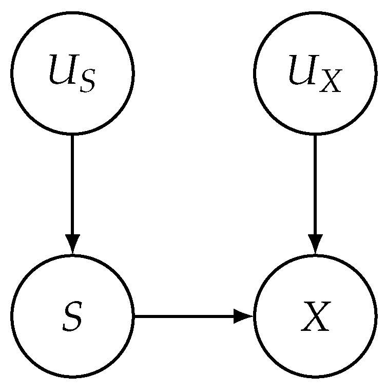
We can specify an appropriate transformation directly, and hence an appropriate norm for and a more sophisticated notion of a counterfactual correlate, by proposing a semantics for counterfactuals in terms of an underlying structural causal model (SCM) [55,56]. An SCM is a graph over a set of endogenous () and exogenous () variable and whose edges represent causal links. These links are specified via equations to determine quantitative effects of changing values of the variables; these equations serve in effect to define endogenous variables in the graph in terms of exogenous ones. With respect to the formalism before, the endogenous variables correspond to dimensions i of the input data space , while the exogenous variables are latent, hidden variables. Such a graph defines the effects of changes on exogenous variables for the endogenous variables leaving the rest constant.
Causal effects are the result of a change or a specification of some set of features or dimensions of an input. Such a change on dimensions I is called a do-intervention on I. Supposing that our SCM G is acyclic and that is some exogenous variable in G then a do intervention on I then defines a change on the other relevant dimensions of X represented by variables that are its children in G. It tells us explicitly how an intervention affects which properties that our focal point may have. In addition, the equations associated with the edges in the SCM can specify probabilities for outcomes.
What is an intervention logically? Our atomic formulas are of the form , where is variable representing a dimension of , and its value. Each instance in can described by an n-ary conjunction of atomic formulas specifying the values of each dimension at that instance. In general, we are evaluating counterfactuals at instances like ’nicholas’ that have the form Had the values of gender been female, then the value of the loan would have been 0, which is an approximation of Had Nicholas been female, he would not have gotten the loan.
An -definable intervention then is a pair of sets definable by a pair of conjunctions of atomic formulae where specifies values for a subset of variables while specifies values . Note that is typically the formula that describes the focal point or set of focal points used for evaluation and so it may set values for more variables than those in S Let be the pair of formulae representing an -definable intervention on S. The set represents the set of all those instances that have the shifted values ; is another conjunctive formula whose interpretation represents the set of all instances in with original values .
In the AI literature, S is typically supposed to be a single variable. But this limits the kinds of counterfactuals we can consider. Single valued interventions can handle counterfactuals where we specify one shifted value like annual income,
- (11)
- Had Nicholas earned €100 K per year (instead of €50 K), he would have gotten the loan.
But it clearly also makes sense to think about and evaluate counterfactuals where we change the values of more than one variable.
- (12)
- Had Nicholas earned €100 K euros per year (instead of €50 K) but lives in a part of the city with this zip code, he would not have gotten the loan.
Generally, then, we will think of an intervention as a shift in the value of any subset S of variables of from their values at the point of evaluation or set of points of evaluation. Given a complete SCM G, an intervention on defines a unique minimally appropriate set valued as defined in Definition 19. Now that we’ve added indeterminism and probability, An SCM G for a given intervention S generates not only a set valued specifying truth conditions but also a probability distribution over the elements in .
We can then exploit these transformations along with the graphs and equations of SCMs in a semantics of counterfactuals following Definition 16. We supply both a truth value and a probability distribution for both individual evaluation points and sets for counterfactuals.
Definition 21.
Let ψ define a set of values for variables in S and let be a counterfactual model with transformations determined by an underlying SCM G. Then:
- just in case:.
- just in case:
- just in case:
- just in case:
In case one has a complete SCM, then one has a theory of counterfactuals that captures the full causal consequences of a do-intervention. A complete SCM for a given problem would seem to provide an ideal explanatory counterfactual model, where counterfactuals are directly tied to causal relations.
As we shall see in the next section, however, our intuitions about counterfactuals show that there may be relevant counterfactuals that are true even when the antecedents do not express variables that are causally operative on the variables expressed in the consequent of the counterfactual. So a causal model might not yield a completely satisfactory semantics of counterfactual statements.
Of course, if we’re interested in explainability, a linguistically optimal theory of counterfactual conditionals is secondary to the adequacy of the explanations provided. And here a causal model seems arguably optimal. The problem is, we almost never have complete SCMs for the problem investigated; and finding such SCMs from data is at least NP hard. So while a counterfactual model based on an SCM might seem ideal it is difficult to attain in practice. We can’t effectively build the model.
Let’s take a closer look at this problem in the case of explaining the behavior of an ML algorithm . Can we just use data and consider as a black box? Yes, but in general this gets us just statistical correlations. How can we test for hidden confounders or causal dependencies when some of the variables in the full causal model are part of ? And what do we mean by causal dependencies when it comes to an ML algorithm? Even if is a sophisticated deep neural net, it is still a Turing machine with a logical theory . encodes a succession of applications of functions, some of them non-linear, to data. In this logical reconstruction , the causal links between data and predictions of become deductively valid relations or relations of logical consequence. So a full causal model in the case of an ML algorithm must characterize the semantic consequences of together with, at the very least, elements from . The SCM then that explains and provides the cause of a prediction is a matter of finding a provably valid relation between a subset or minimal set of feature values and the prediction. Namely, we have to prove: But this problem is already hard when is a binary classifier [57]. This problem becomes completely insoluble when we have to reason about probabilities, as the underlying logic used to encode becomes typically non-axiomatizable [54]. We don’t see frankly how it’s plausible to suppose that one can build a full SCM for a sophisticated ML algorithm.
Thus, the causal approach, attractive as it seems, is also difficult to implement. What we need a notion of an intervention that gives us a sophisticated notion of counterfactual counterparts but that is not tied to the presence of a complete SCM. This is what we shall find in the next Section 7.2.
7.2. Transport Counterfactual Models
In this section we sketch a view of Transport theory that provides counterfactual models that remedy the problem we just mentioned. A transport based counterfactual model can provide a sophisticated notion of counterfactual correlates and a fortiori interesting transformations in the absence of an underlying SCM. Ref. [50] define what we shall call a counterfactual operation (Ref. [50] call it a model but we will reserve this term for the logical structure providing truth conditions we define below.) in terms of a coupling of two distributions that itself depends on an intervention , where and specify values and respectively of the variables in S, and we consider an intervention in S. Suppose we observe two different distributions , whose support are the sets and We now seek to discover what are the “best” in some sense to be determined counterfactual correlates for . Transport theory tells us that a counterfactual counterpart in of some element verifying should respect the distributions that and support.
A coupling between two distributions P and is a probability on whose first projection is P and second projection is ; i.e., and for measurable sets . Over finite sets, A, B, we can write and . A coupling then in such a case must obey the following constraint [58]:
Given this constraint, we see a coupling as a matrix in the finite case over elements in the finite sets A and B. Let be the set of such couplings. In some sense this is the essence of the general problem of finding counterfactual counterparts.
But there are many such couplings. Which one should we choose? In the discrete case, once we have a cost function for building the coupling , finding an optimal transport plan requires solving this optimisation problem:
In the continuous case, Equation (3) becomes the optimisation problem as formulated by Kantorovich:
Solutions to (3) and (4) are optimal transport plans between and with respect to c. As long as c any non negative distance function on the space we are in effect minimizing something equivalent to a Wasserstein distance over distributions. Linking this to counterfactual semantics brings a very different viewpoint to counterfactual correlates. Nevertheless, we note that the choice of c will bring support different counterfactual theories.
Following [50], we link couplings to do-interventions in the following way. Suppose an intervention , where specifies values and specifies for the variables in S, and two observable distributions with supports and . A counterfactual operation given such an intervention is a coupling that pairs elements with elements such that the projection requirements for couplings are preserved. Given an intervention , is a pairing of elements of with , each with their own marginal probabilities that get a score.
Concretely, this means that if x has a property like a salary of €100 K euros per year and the probability of having such a salary given that one is a is —e.g., , then should have a salary M such that . Moreover this correspondence between x and should be maximized for every property .
We are particularly interested in random couplings where x may have several counterparts , each assigned a probability. Using a random coupling allows for multiple counterfactual counterparts of a single instance, as in Lewis’s original semantics. It means that the logic doesn’t verify conditional excluded middle, which we’ve argued is unintuitive when we consider situations in which an intervention only has a limited effect. We will group together the counterparts of x under the coupling with the term . We use to build a semantics for counterfactuals [59].
The random couplings of two distributions that are solutions to (3) or (4) in effect furnish the transport minimal adequate transformations for our model. In the finite case, relative to an optimal tranport plan we can define for
In other words, we collect all the elements in that are paired via a non 0 probability with a given w via the coupling.
How does the transformation we just defined in Equation (5) relate to our counterfactual models for ? In effect, Equation (5) defines just the counterfactual counterparts and the appropriate transformations in a counterfactual model . In addition, however, We can exploit the coupling and the intervention it is related to to give a more sophisticated semantics for the probability of a counterfactual.
Definition 22.
A transport counterfactual model extends a counterfactual model with a set of interventions or set of pairs of definable sets , , and a set of couplings with support A and B that are solutions to Equation (4) over distributions ; i.e., is a set of optimal transport plans.
We will assume that (4) has a unique solution.
Definition 23.
The transport semantics for counterfactuals:
- just in case:
- just in case:
- just in case:
- just in case:
Note that our semantics allows us to set a set of evaluation points Z to for instance.
We examine some more consequences of the counterfactual semantics from transport models below.
7.2.1. Six Advantages of Transport Based Counterfactual Models
Transport plans are practically appealing and have been extensively exploited in many applications involving data fusion, like the fusion of data from different sources. They also have a number of advantages for a theory of counterfactuals and the explainability of ML algorithms. Here we list six: the tractability of the model construction, increased explanatory relevance, improving efficiency of finding relevant logically valid explanations, providing explanations with partial or fragmentary data, testing for biases at a non local level of the model, and increased robustness of the underlying classifier when transport based methods are used.
Tractability of the model construction. Unlike the case of our models built on causal SCMs, we can always build a counterfactual model based on a transport approach. In addition, transport techniques work over sets of instances or subsets of and so in principle are more effective than constructing counterfactual models pointwise from adversarial perturbations. In certain cases (where each coupling determines a unique counterfactual counterpart for each instance), computing an optimal transport plan can be found in polynomial time relative to the size of samplings on the distributions and [18,21,60,61]. Thus the models can be determined in polynomial time irrespective of the size of the implementation of the learning architecture, though for very large dimensional data sets the method may lead to complications. Even without the deterministic assumption, there are also relatively efficient implementations for approximating optimal transport plans and building a counterfactual model [62,63].
Increased explanatory relevance. Counterfactual transport-based models can not only be reliably constructed but they are also more explanatorily relevant for explaining ML behavior than our generic counterfactual models. Transport theories furnish, as [59] pointed out, counterfactual correlates given some intervention on an instance x that match each other as closely as possible in terms of probability distributions. Compare this to a counterfactual counterpart of x in which just one property is shifted without regard to distributions. Given an intervention , we’ve seen earlier in Section 6.1 a thought experiment in which simply shifting one property of x who is a typical can yield a a very atypical counterpart . We might expect our algorithm to be sensitive to atypicality; ’s predictions about very atypical cases would typically be out of the domain distribution; they might not even be physically possible in some extreme cases. And so we might expect to provide unreliable results on such instances. In any case such atypical counterparts seem far less relevant for an explanation of the behavior of on a typical, real life example x than counterparts of x that are also typical. So, if we want to see whether a shift from to is explanatorily relevant to the behavior of at a typical x, we should first look at how treats typical instances . Thus, transport models should be extremely explanatorily relevant for many queries about behavior.
More efficient searches for relevant, logically valid explanations. Transport based counterfactual models allow us to be more efficient in providing logically valid explanations. Why is this? First, we note:
Remark 4.
Given supported by a coupling , and where for and is the theory or logic encoding of , we can effectively find a minimal subformula χ of s.th. offers a logically valid, abductive explanation in the sense of [4]).
Remark 4, whose proof just repeats that of Proposition 2, provides a logical guarantee of the explanation provided by the counterfactual. That is, it allows us to transform a local, partial, counterfactual explanation into a global, valid, deductive explanation.
Our transport based models endow counterfactuals with probabilities and allow us to evaluate counterfactuals not only at the local level but at more global levels in the model, relative to various sets of instances. This is something we have not seen at least explicitly developed in other approaches to explainability in the literature. And because transport models assign counterfactuals probabilities based on observed distributions, we can target higher probability counterfactuals for logical investigation.
More precisely, since we can estimate the probabilities of counterfactual conditionals over sets of instances in , higher probability counterfactuals should be a priori more relevant to the explainee; they are the ones that hold of a greater proportion of the data. As such they are also more relevant for investigating the ML algorithm , as high probability counterfactuals capture how performs over large parts of the data set. In addition, we can further restrict our search for globally and logically valid explanations, i.e., the technique in Proposition 4, to those with the highest global probability. Given that testing for logically valid explanations is computationally expensive, restricting our search in this way can be very useful. Using this probabilistic information can also help us restrict our search for relevant counterfactuals in the pragmatic component of explanations that we dicussed in Section 4.
Non local testing for biases and confounders. Another important advantage of transport counterfactual models is that we can test for confounders and biases for or against members of some subset as in Remark 3 at a more global and representative level. Once again, examining biases at a global level of an ML algorithm is important for gauging the behavior of ; if is biased on certain outliers in , outliers that may be artifacts and not represent any real world cases, then that is less serious than if has biases on typical members of P.
As in Remark 3, we want to know whether is sensitive to values of variables that define, perhaps implicitly, a certain subset P of , which we will represent by a Boolean formula . We say that iff . Then:
Remark 5.
Let be a forcing explanation investigation game where consists of those plays in which establishes whether for and . Suppose in addition that has access to the distribution in the transport counterfactual model and the coupling . Then has a winning strategy in in polynomial time.
To establish Remark 3, we simply note that to establish a bias for or against P it is necessary but also sufficient to look at representative examples of P. can request those that provide those representative examples by exploiting facts about and .
Providing explanations with partial or fragmentary data. A fifth advantage of transport based counterfactual models is that their capability of set evaluation has important consequences for explaining the behavior of ML models when we have only partial data. (This could also apply to causally based models as we developed them in Section 7.1.) Suppose we want to explain the predictions of an ML algorithm on certain individuals predictions for whom we only have partial data. This means in effect that we want to evaluate counterfactuals over sets of instances that verify the partial data entries we have. Because our semantics allows for this—indeed transport approaches intuitively ask us to do this—such counterfactual models are natural candidates to explore ML behavior in cases of partial data.
Increased robustness. A last advantage of transport based models is that using transport based models for ML can lead to more robust performance. Ref. [64] show that one can use a variant of Equation (2) to train an ML classifier. That is, we can use the basis of the transport based counterfactual model for the ML system itself. Ref. [22] show that while such a classifier doesn’t perform very well, by adding constraints on the classifier such that it must respect Lipschitz continuity properties and using a hinge loss one can achieve a classifier that has state of the art performance but one that has very interesting robustness properties. In particular, what they show is that adversarial attacks on such a classifier only succeed if they provide counterfactual counterparts sanctioned by the transport model. And this means that an attack a can only force if obeys the distributions that one would expect of a typical member of the other class. Thus, the attacks result in per se interpretable shifts of the behavior of . This point needs much more exploration but potentially conveys a very exciting development for transport based classifiers and their explanatory models.
7.2.2. Transport-Based Models, Counterfactual Conditionals and Salmon Explanatory Relevance
In this section, we explore how transport based models affect predictions about counterfactual conditionals. As far as we know, this paper is the first paper to link transport based approaches to counterfactuals with semantic and logical approaches. This allows us to investigate the semantic implications of transport based models. The semantics for counterfactuals within transport based models bears many resemblances to the probabilistic semantics we’ve already introduced. For instance, a transport counterfactual model with a random coupling won’t necessarily support conditional excluded middle or the examples given in example (6). But it could support:
- (13)
- Had Nicholas chosen to work in industry, the chances that he would have had a salary of €100 K would be much higher.
On the other hand, the assignment of probabilities and truth conditions to counterfactuals in transport models is more sophisticated than in a generic probabilistic model because it exploits the coupling of two distributions. The distance function used to compute counterparts differs from any precisification of Lewisian similarity that proposed so far to our knowledge, because it exploits not only the semantics of the antecedent of the counterfactual but also the probability distribution that it supports and compares that distribution to the one at the point of evaluation. What this means in practice is that, for instance, (7) will be true at a world only if at the worlds coupled with the chances of having a salary of €100 K given that one works in industry are as close as possible to those of having having a salary of €100 K given that one works in industry in the evaluation points (data points) where we have data about industry workers. Moroever those chances should be far higher than the chance of Nicholas having a salary of €100 K given his actual occupation. We find these linguistic consequences of the model very plausible.
Transport counterfactual models conform to our intuitions about distributions—namely, that a counterfactual model based on an intervention should respect observed distributions concerning that intervention. This also makes predictions about counterfactual statements. Consider again the counterfactual assumption that I make €100 K euros a year instead of €60 K euros a year. My closest counterparts should take part in the distributions of €100 K a year earners in as close a possible a way as I take part in the distributions €60 K a year earners. This is what the transport semantics guarantees.
Transport models entail a kind of probabilistic inertia that enables them to capture a wide variety of counterfactual conditionals. In particular it enables them to make true causally supported counterfactuals. But it also makes other counterfactuals true as well. Consider a typical confounder case: grey haired people are more likely to get heart attacks, but of course grey hair is not a cause of heart attacks. Consider the intervention where we change hair color. Grey haired people are on average much older than non grey haired people, so a grey haired counterfactual counterpart of a brunette twenty five year old should be considerably older under an optimal transport plan. In a transport counterfactual model, we thus predict the truth of
- (14)
- Were you to be grey haired, you would be more likely to have a heart attack.
Many people in fact accept the truth of (14), despite knowing that having grey hair doesn’t cause heart attacks. This in itself shows that perhaps counterparts that are solely based on causal graphs are not correct, since a causal theory would not draw a causal link between having grey hair and having a heart attack; and thus, counterparts defined via an SCM would not necessarily have a higher probability of having a heart attack and so such a model would predict that (14) is false. If people object to (14) it may be because they have another intervention in mind that the antecedent of (14) evokes. This is the intervention: grey haired and same age—which a transport model also supports. In this case, we can look at the rate of heart attacks across the grey haired say 25 to 50 year olds and the factual distribution should tell us that are much lower than the rate of heart attacks across the grey haired 50 to 80 year olds. On this intervention, (14) is not predicted to be true.
This points to a deeper connection between counterfactuals, explanations and distribution preservation. Ref. [65] noted that while statistical relevance is a property that is relevant to explanatory goodness, it’s not sufficient. Salmon argued that what we needed for a good explanation for why for some b has A, was what he calls a homogeneous partition of B:
Definition 24.
is a homogeneous partition of B with respect to A iff
- 1.
- is a partition of B;
- 2.
- 3.
- there is no finer partition of B meeting this condition.
A homogeneous partition of B relative to some property A provides all the statistically relevant factors for A. Salmon proposes the following definition of an adequate explanation.
Definition 25.
is Salmon explanatorily relevant to why b in class B has property A iff:
- 1.
- there is a homogeneous partition of B with respect to A with
- 2.
- 3.
- for .
We note that one can have several homogeneous partitions that meet the conditions in Definition 25.
Let’s now explore how this links up to transport counterfactual models. The probabilistic inertia of counterfactual models provides the information necessary to construct homogeneous partitions and explanatory relevance. Recall our hair-color-change example above. Interventions can lead to true counterfactuals supported only by statistical relevance, but other interventions, more specific interventions, where we control for other important variables like age, can remove confounders to capture explanatory relevance and approximate better the true causes of the observed distributions. This notion of specificity is definable in our models:
Definition 26.
An intervention is more specific than an intervention if .
This allows us to define straightforwardly homogeneous partitions in Salmon’s sense and to capture explanatory relevance. Note that establishing that one intervention is more specific than another can be determine in linear time in the worst case with respect to the size of the description of the sets.
Remark 6.
Given with intervention , we can effectively check whether is Salmon explanatorily relevant.
Similarly to the proof idea in Remark 4, we can check whether is the most specific intervention (specificity can be computed in linear time) that supports . But in addition, where , are alternative instantiations for the variables in to , we need to establish for explanatory relevance: . Given that a transport model carries probability information for all measurable and so all definable sets in , the complexity of establishing explanatory relevance is bounded by the search for the appropriate distributions.
Finally, the fact that our semantics allows us to analyze counterfactuals supported by sets of evaluation points and so, for example, a group whose counterfactual properties we want to examine. This allows us to analyze sentences about groups like
- (15)
- If members of a disfavored minority were treated like a favored minority, their chances of getting loans would be far higher.
7.2.3. Transport and Causality
Transport counterfactual models show us a rich set of counterfactual relations. Some relations are supported by statistical relevance; others by explanatory relevance, and still others by causal mechanisms like those encoded in SCMs. To some extent this may be due to the choice of the cost function c. Nevertheless, we think this is not simply a fortuitous coincidence but rather a consequence of what an optimal transport plan should do.
Under certain assumptions, Ref. [50] show that the counterfactuals verified by transport model are just those supported by a particular kind of SCM, thus providing a theoretical underpinning to [59] who empirically observed a close similarity between counterfactual theories based on transport models to those based on causal models. While there are several technical assumptions concerning the ground cost (c) in Equation (4) and on the distributions involved in the transport, we look here at two assumptions on SCMs. The first assumption is that the equations on the edges of the graph induce a one-to-one correspondence between endogenous and exogenous variables. The second is a constraint they call relative exogeneity (RE). To state this constraint, recall that we are interested in an SCM in a set S of endogenous variables that we may exploit in an intervention and which are distinct from the rest of the endogenous variables X of the SCM. Where are the exogenous parents of S and X respectively and is the set of endogenous variables that are parents of S, RE requires: and (Figure 2). This entails that there is no hidden confounder between X and S and no variable in X is a direct cause of S. We note that [50] also restrict S to a singleton set.
RE rules out confounder cases like those that support counterfactuals like (14). Example (14) holds because of the causal relation between the variable age and the probability of heart attacks. If age is in X then it is a direct cause of a change in hair color (the S in that example) and if it is not, it is a hidden confounder and so also ruled out.
Because a transport model links distributions across all measurable sets, an optimal plan will make true counterfactuals that rely on statistical correlations due to confounders. It will also be the case that a statistical correlation between the true cause and its true effect will also be preserved by the coupling in the sense that we elucidated above. But what about the counterfactuals involving those confounders? Does a coupling supporting a counterfactual have a natural relation to the coupling ,where is a confounder of ?
The answer in general is “no”, because doesn’t entail . Counterfactuals don’t in general obey conditional transitivity. If we enforce conditional transitivity in general, we threaten to make counterfactuals semantically equivalent to material conditionals or strict conditionals, something that would vitiate the whole approach. On the other hand, suppose we know that is a necessary and sufficient cause of ; that is, is sufficient for producing on its own, and does not occur without (meaning that is necessary for ).
Proposition 8.
Suppose that ζ is a necessary and sufficient cause of ψ in . Then if , then .
Proof.
Let be a necessary and sufficient cause of . Formally, this means , since ’s being a necessary cause of in is defined by and being a sufficient cause means . Now suppose that we are interested in prediction at a point w, we have . Given , this means that every closest world is also a closest world. So if , then . □
If the conditions of Proposition 8 hold, then the causally grounded counterfactual is supported along with . With transport models we are also conferring probabilities on outcomes, however. So can we have a probabilistic counterpart of Proposition 8? In addition, is there a cost function such that there is an optimal transport plan meeting (4) that would yield such a result?
Remark 7.
The set of counterfactuals made true at in a transport counterfactual model include causally relevant counterfactuals for all necessary and sufficient causes in the sense of Proposition 8. When an SCM obeys RE, it generates a (not necessarily optimal) transport counterfactual model that includes all counterfactuals supported by the SCM.
7.2.4. Some Thoughts on Logic and Probability in Transport Counterfactual Models
In the counterfactual models where formulas can be assigned probabilities as well as truth values at evaluation points or sets of evaluation points, it is still nevertheless the case that the logical or truth semantic and statistical inferencing mechanisms are separate. But they can also cooperate. We can use statistical techniques to estimate probabilities of conditionals and to construct appropriate couplings and transport plans and then investigate high probability counterfactual explanations for logical validity and examine other properties of transport models with logic. We can also exploit the techniques of Section 3 to investigate the flip degree of transport models.
Our approach contrasts with many neuro-symbolic proposals in which the logic is not autonomous and there are no guarantees that logical consequence is preserved during the operation of the system [66]. There are also problematic assumptions (independence) about probabilities when imported into logical frameworks as in [66]. We do not derive logical inferences from statistical ones nor statistical patterns of inference or assumptions about the statistics from logical notions. Ref. [67]’s criterion that both systems work according to their usual rules holds here. Nevertheless, they can cooperate as we have tried to show. In effect the axioms for counterfactuals of [16] hold in our models as the transport plans are used solely to determine counterfactual counterparts, if we only look at the Boolean values for counterfactuals and ignore the probability assignments to them given by the couplings. However, the transport coupling also confers a probability on counterfactuals. Given [54]’s results, reasoning logically about probabilities in this framework remains unaxiomatizable.
8. Conclusions
We have shown that counterfactual explanations can deliver partial, but epistemically accessible and adequate explanations. We have also shown linked counterfactual explanations to valid deductive explanations. We have also looked at a range of counterfactual models—from one relying on a simple edit or Manhattan distance to compute counterfactual counterparts, to models based on structural causal graphs, and finally to sophisticated models that rely on theories of transport. We have argued that transport models hold great promise for explanatory relevance, and as far as we know we are the first to link transport based ideas to a logical theory of counterfactuals and its semantics. This paper is also the first, we believe, to outline the many advantages of transport based counterfactual models for the explainability of ML algorithms. We have enumerated six advantages—the tractability of the model construction, increased explanatory relevance, improving efficiency of finding relevant logically valid explanations, providing explanations with partial or fragmentary data, testing for biases at a non local level of the model, and increased robustness of the underlying classifier when transport based methods are used. There are probably many more. In addition, we’ve seen how transport based models can capture some causal information in the absence of an SCM.
Another important take-away message from this paper is that for all counterfactual models, pragmatic factors are crucial. We have proved for the simplest counterfactual models that pragmatic factors dramatically affect the complexity of finding adequate explanations. We reviewed Explanation Games from [15], which allowed us to characterize the problem of finding fair and adequate counterfactual explanations for a ML classifier with Boolean valued features as a PLS complete search problem. In addition, we explored how the complexity of the set of counterfactuals describing a local neighborhood around a focal point can affect both the complexity of fair and adequate explanations and our evaluation of the learning algorithm as a model. While these results are proved only for the simplest of counterfactual models, we believe they set lower computational bounds for finding fair and adequate explanations in the more complex models like transport based ones.
Additionally in this paper, we have extended explanation games beyond previous work to explore the counterfactual model itself. With the more sophisticated counterfactual models, we have been able to explore the complexity of biases at a more global level of the model, not just locally. And we have been able to formulate how to check for biases with respect to representative samples of protected classes.
In future work we need to explore with experiments whether and if so how the theoretical advantages we have outlined here for counterfactual explanations, in particular those based on transport models, translate into empirical gains for explainability and for the efficiency of finding fair and adequate explanations. We will look at efficient heuristics for this step. We will also look at how explanation games help us to formally explore interactive machine learning, in particular “human in the loop” or interactive explainability for machine learning function behavior [68,69]. Such game theoretic investigations may have special relevance in medical domains [70].
Author Contributions
Conceptualization: N.A. and C.R.; Formal analysis: N.A., L.D.L. and S.P.; writing—original draft preparation: N.A.; writing—review and editing: N.A., L.D.L. and S.P. All authors have read and agreed to the published version of the manuscript.
Funding
The ANR PRCI grant SLANT, the ICT 38 EU grant COALA and the 3IA Institute ANITI funded by the ANR-19-PI3A-0004 grant provided research support.
Institutional Review Board Statement
Not applicable.
Informed Consent Statement
Not applicable.
Data Availability Statement
The data presented in this study are available in article.
Acknowledgments
We thank the ANR PRCI grant SLANT, the ICT 38 EU grant COALA and the 3IA Institute ANITI funded by the ANR-19-PI3A-0004 grant for research support. We also thank the reviewers for their insightful comments.
Conflicts of Interest
The authors declare no conflict of interest.
References
- Ribeiro, M.T.; Singh, S.; Guestrin, C. “Why Should I Trust You?”: Explaining the Predictions of Any Classifier. In Proceedings of the 22nd ACM SIGKDD International Conference on Knowledge Discovery and Data Mining, San Francisco, CA, USA, 13–17 August 2016; pp. 1135–1144. [Google Scholar]
- Ribeiro, M.T.; Singh, S.; Guestrin, C. Anchors: High-Precision Model-Agnostic Explanations. In Proceedings of the AAAI Conference on Artificial Intelligence, New Orleans, LA, USA, 2–7 February 2018; pp. 1527–1535. [Google Scholar]
- Wachter, S.; Mittelstadt, B.; Russell, C. Counterfactual Explanations without Opening the Black Box: Automated Decisions and the GPDR. Harv. JL Tech. 2017, 31, 841. [Google Scholar] [CrossRef] [Green Version]
- Ignatiev, A.; Narodytska, N.; Marques-Silva, J. On Relating Explanations and Adversarial Examples. In Advances in Neural Information Processing Systems; NeurIPS: Vancouver, BC, Canada, 2019. [Google Scholar]
- Bachoc, F.; Gamboa, F.; Halford, M.; Loubes, J.M.; Risser, L. Entropic Variable Projection for Explainability and Intepretability. arXiv 2018, arXiv:1810.07924. [Google Scholar]
- Rathi, S. Generating counterfactual and contrastive explanations using SHAP. arXiv 2019, arXiv:1906.09293. [Google Scholar]
- Murdoch, W.J.; Singh, C.; Kumbier, K.; Abbasi-Asl, R.; Yu, B. Definitions, methods, and applications in interpretable machine learning. Proc. Natl. Acad. Sci. USA 2019, 116, 22071–22080. [Google Scholar] [CrossRef] [PubMed] [Green Version]
- Simonyan, K.; Vedaldi, A.; Zisserman, A. Deep inside convolutional networks: Visualising image classification models and saliency maps. arXiv 2013, arXiv:1312.6034. [Google Scholar]
- Kusner, M.J.; Loftus, J.; Russell, C.; Silva, R. Counterfactual fairness. In Advances in Neural Information Processing Systems; NeurIPS: Long Beach, CA, USA, 2017; pp. 4066–4076. [Google Scholar]
- Bromberger, S. An Approach to Explanation. In Analytical Philsophy; Butler, R., Ed.; Oxford University Press: Oxford, UK, 1962; pp. 72–105. [Google Scholar]
- Achinstein, P. The Nature of Explanation; Oxford University Press: Oxford, UK, 1980. [Google Scholar]
- Miller, T. Explanation in artificial intelligence: Insights from the social sciences. Artif. Intell. 2019, 267, 1–38. [Google Scholar] [CrossRef]
- Holzinger, A.; Carrington, A.; Müller, H. Measuring the quality of explanations: The system causability scale (SCS). KI-Künstliche Intell. 2020, 34, 1–6. [Google Scholar] [CrossRef] [Green Version]
- Verma, S.; Dickerson, J.; Hines, K. Counterfactual explanations for machine learning: A review. arXiv 2020, arXiv:2010.10596. [Google Scholar]
- Asher, N.; Paul, S.; Russell, C. Fair and Adequate Explanations. In International Cross-Domain Conference for Machine Learning and Knowledge Extraction; Springer: Berlin/Heidelberg, Germany, 2021; pp. 79–97. [Google Scholar]
- Lewis, D. Counterfactuals; Basil Blackwell: Oxford, UK, 1973. [Google Scholar]
- Younes, L. Diffeomorphic Learning. arXiv 2018, arXiv:1806.01240. [Google Scholar]
- Cuturi, M. Sinkhorn distances: Lightspeed computation of optimal transport. In Proceedings of the Advances in Neural Information Processing Systems, Lake Tahoe, NV, USA, 5–10 December 2013; pp. 2292–2300. [Google Scholar]
- Kurakin, A.; Goodfellow, I.; Bengio, S. Adversarial examples in the physical world. arXiv 2016, arXiv:1607.02533. [Google Scholar]
- Dube, S. High dimensional spaces, deep learning and adversarial examples. arXiv 2018, arXiv:1801.00634. [Google Scholar]
- Peyré, G.; Cuturi, M. Computational Optimal Transport: With Applications to Data Science. Found. Trends® Mach. Learn. 2019, 11, 355–607. [Google Scholar] [CrossRef]
- Serrurier, M.; Mamalet, F.; González-Sanz, A.; Boissin, T.; Loubes, J.M.; del Barrio, E. Achieving robustness in classification using optimal transport with hinge regularization. In Proceedings of the IEEE/CVF Conference on Computer Vision and Pattern Recognition, Nashville, TN, USA, 20–25 June 2021; pp. 505–514. [Google Scholar]
- Fan, X.; Toni, F. On Computing Explanations in Argumentation. In Proceedings of the Twenty-Ninth AAAI Conference on Artificial Intelligence, Austin, TX, USA, 25–30 January 2015; pp. 1496–1502. [Google Scholar]
- Ignatiev, A.; Narodytska, N.; Marques-Silva, J. On validating, repairing and refining heuristic ML explanations. arXiv 2019, arXiv:1907.02509. [Google Scholar]
- Friedrich, G.; Zanker, M. A taxonomy for generating explanations in recommender systems. AI Mag. 2011, 32, 90–98. [Google Scholar] [CrossRef] [Green Version]
- Bach, S.; Binder, A.; Montavon, G.; Klauschen, F.; Müller, K.R.; Samek, W. On pixel-wise explanations for non-linear classifier decisions by layer-wise relevance propagation. PLoS ONE 2015, 10, e0130140. [Google Scholar] [CrossRef] [Green Version]
- Nam, W.J.; Gur, S.; Choi, J.; Wolf, L.; Lee, S.W. Relative attributing propagation: Interpreting the comparative contributions of individual units in deep neural networks. In Proceedings of the AAAI Conference on Artificial Intelligence, Vancouver, BC, Canada, 2–9 February 2020; Volume 34, pp. 2501–2508. [Google Scholar]
- Hempel, C.G. Aspects of Scientific Explanation; Free Press: New York, NY, USA, 1965. [Google Scholar]
- Ignatiev, A.; Narodytska, N.; Asher, N.; Marques-Silva, J. On Relating “Why?” and “Why Not?” Explanations. arXiv 2020, arXiv:2012.11067. [Google Scholar]
- Molnar, C. Interpretable Machine Learning. Lulu. com. Available online: http://leanpub.com/interpretable-machine-learning2019 (accessed on 12 March 2020).
- Doshi-Velez, F.; Kim, B. Towards a rigorous science of interpretable machine learning. arXiv 2017, arXiv:1702.08608. [Google Scholar]
- Lewis, D. Causation. J. Philos. 1973, 70, 556–567. [Google Scholar] [CrossRef]
- Gärdenfors, P.; Makinson, D. Revisions of Knowledge Systems Using Epistemic Entrenchment. In Proceedings of the Second Conference on Theoretical Aspects of Reasoning about Knowledge, Pacific Grove, CA, USA, 7–9 March 1988; Vardi, M.Y., Ed.; Morgan Kaufmann: San Francisco, CA, USA, 1988; pp. 83–95. [Google Scholar]
- Williamson, T. First-order logics for comparative similarity. Notre Dame J. Form. Log. 1988, 29, 457–481. [Google Scholar] [CrossRef]
- Salzberg, S. Distance metrics for instance-based learning. In International Symposium on Methodologies for Intelligent Systems; Springer: Berlin/Heidelberg, Germany, 1991; pp. 399–408. [Google Scholar]
- Ignatiev, A.; Narodytska, N.; Marques-Silva, J. Abduction-based explanations for machine learning models. In Proceedings of the AAAI Conference on Artificial Intelligence, Honolulu, HI, USA, 27 January–1 February 2019; pp. 1511–1519. [Google Scholar]
- Karimi, A.H.; Barthe, G.; Balle, B.; Valera, I. Model-agnostic counterfactual explanations for consequential decisions. In Proceedings of the International Conference on Artificial Intelligence and Statistics, Sicily, Italy, 26–28 August 2020; pp. 895–905. [Google Scholar]
- Laugel, T.; Lesot, M.J.; Marsala, C.; Renard, X.; Detyniecki, M. Unjustified classification regions and counterfactual explanations in machine learning. In Proceedings of the Joint European Conference on Machine Learning and Knowledge Discovery in Databases, Würzburg, Germany, 16–20 September 2019; pp. 37–54. [Google Scholar]
- Lundberg, S.M.; Lee, S. A Unified Approach to Interpreting Model Predictions. In Proceedings of the Neural Information Processing Systems, Long Beach, CA, USA, 4–7 December 2017; pp. 4765–4774. [Google Scholar]
- Chang, C.C.; Keisler, H.J. Model Theory; Elsevier: Amsterdam, The Netherlands, 1990. [Google Scholar]
- Junker, U. Preferred explanations and relaxations for over-constrained problems. In Proceedings of the Nineteenth National Conference on Artificial Intelligence, San Jose, CA, USA, 25–29 July 2004. [Google Scholar]
- Slack, D.; Hilgard, S.; Jia, E.; Singh, S.; Lakkaraju, H. Fooling LIME and SHAP: Adversarial Attacks on Post hoc Explanation Methods. In Proceedings of the AIES ’20: AAAI/ACM Conference on AI, Ethics, and Society, New York, NY, USA, 7–8 February 2020; pp. 180–186. [Google Scholar]
- Ginsberg, M.L. Counterfactuals. Artif. Intell. 1986, 30, 35–79. [Google Scholar] [CrossRef]
- Pearl, J. System Z: A natural ordering of defaults with tractable applications to nonmonotonic reasoning. In Proceedings of the 3rd Conference on Theoretical Aspects of Reasoning about Knowledge (TARK’90), Beijing, China, 25–27 June 1990; pp. 121–135. [Google Scholar]
- Spence, A.M. Job Market Signaling. J. Econ. 1973, 87, 355–374. [Google Scholar] [CrossRef]
- Johnson, D.S.; Papadimitriou, C.H.; Yannakakis, M. How easy is local search? J. Comput. Syst. Sci. 1988, 37, 79–100. [Google Scholar] [CrossRef] [Green Version]
- Papadimitriou, C.H.; Schäffer, A.A.; Yannakakis, M. On the complexity of local search. In Proceedings of the Twenty-Second Annual ACM Symposium on Theory of Computing, Baltimore, MD, USA, 13–17 May 1990; pp. 438–445. [Google Scholar]
- Asher, N.; Paul, S. Strategic conversation under imperfect information: Epistemic Message Exchange games. Logic Lang. Inf. 2018, 27, 343–385. [Google Scholar] [CrossRef] [Green Version]
- Alvarez-Melis, D.; Jaakkola, T.S. On the robustness of interpretability methods. arXiv 2018, arXiv:1806.08049. [Google Scholar]
- De Lara, L.; González-Sanz, A.; Asher, N.; Risser, L.; Loubes, J.M. Transport-based Counterfactual Models. arXiv 2021, arXiv:2108.13025. [Google Scholar]
- Halpern, J.Y. An analysis of first-order logics of probability. Artif. Intell. 1990, 46, 311–350. [Google Scholar] [CrossRef]
- Bacchus, F.I. Representing and Reasoning with Probabilistic Knowledge; MIT Press: Cambridge, MA, USA, 1989. [Google Scholar]
- Fagin, R.; Halpern, J.Y. Reasoning about knowledge and probability. J. ACM (JACM) 1994, 41, 340–367. [Google Scholar] [CrossRef]
- Abadi, M.; Halpern, J.Y. Decidability and expressiveness for first-order logics of probability. Inf. Comput. 1994, 112, 1–36. [Google Scholar] [CrossRef] [Green Version]
- Spirtes, P.; Glymour, C.N.; Scheines, R.; Heckerman, D. Causation, Prediction, and Search; MIT Press: Cambridge, MA, USA, 2000. [Google Scholar]
- Pearl, J. Causality; Cambridge University Press: Cambridge, UK, 2009. [Google Scholar]
- Wäldchen, S.; MacDonald, J.; Hauch, S.; Kutyniok, G. The Computational Complexity of Understanding Binary Classifier Decisions. J. Artif. Intell. Res. 2021, 70, 351–387. [Google Scholar] [CrossRef]
- Mérigot, Q.; Oudet, E. Discrete optimal transport: Complexity, geometry and applications. Discret. Comput. Geom. 2016, 55, 263–283. [Google Scholar] [CrossRef] [Green Version]
- Black, E.; Yeom, S.; Fredrikson, M. FlipTest: Fairness Testing via Optimal Transport. In Proceedings of the 2020 Conference on Fairness, Accountability, and Transparency, Barcelona, Spain, 27–30 January 2020; Association for Computing Machinery: New York, NY, USA, 2020; pp. 111–121. [Google Scholar] [CrossRef] [Green Version]
- Dvurechensky, P.; Gasnikov, A.; Kroshnin, A. Computational optimal transport: Complexity by accelerated gradient descent is better than by Sinkhorn’s algorithm. Int. Conf. Mach. Learn. 2018, 26, 1367–1376. [Google Scholar]
- Genevay, A.; Chizat, L.; Bach, F.; Cuturi, M.; Peyré, G. Sample complexity of sinkhorn divergences. In Proceedings of the International Conference on Artificial Intelligence and Statistics, Naha-shi, Japan, 16–18 April 2019; pp. 1574–1583. [Google Scholar]
- Pooladian, A.A.; Niles-Weed, J. Entropic estimation of optimal transport maps. arXiv 2021, arXiv:2109.12004. [Google Scholar]
- Seguy, V.; Damodaran, B.B.; Flamary, R.; Courty, N.; Rolet, A.; Blondel, M. Large-scale optimal transport and mapping estimation. arXiv 2017, arXiv:1711.02283. [Google Scholar]
- Arjovsky, M.; Chintala, S.; Bottou, L. Wasserstein generative adversarial networks. In Proceedings of the International Conference on Machine Learning, Sydney, Australia, 6–11 August 2017; pp. 214–223. [Google Scholar]
- Salmon, W.C. Scientific Explanation and the Causal Structure of the World; Princeton University Press: Princeton, NJ, USA, 1984. [Google Scholar]
- De Raedt, L.; Dumančić, S.; Manhaeve, R.; Marra, G. From statistical relational to neuro-symbolic artificial intelligence. arXiv 2020, arXiv:2003.08316. [Google Scholar]
- Poole, D. Logic, probability and computation: Foundations and issues of statistical relational AI. In Proceedings of the International Conference on Logic Programming and Nonmonotonic Reasoning, Vancouver, BC, Canada, 16–19 May 2011; pp. 1–9. [Google Scholar]
- Amershi, S.; Cakmak, M.; Knox, W.B.; Kulesza, T. Power to the people: The role of humans in interactive machine learning. Ai Mag. 2014, 35, 105–120. [Google Scholar] [CrossRef] [Green Version]
- Holzinger, A.; Plass, M.; Kickmeier-Rust, M.; Holzinger, K.; Crişan, G.C.; Pintea, C.M.; Palade, V. Interactive machine learning: Experimental evidence for the human in the algorithmic loop. Appl. Intell. 2019, 49, 2401–2414. [Google Scholar] [CrossRef] [Green Version]
- Holzinger, A.; Malle, B.; Saranti, A.; Pfeifer, B. Towards multi-modal causability with Graph Neural Networks enabling information fusion for explainable AI. Inf. Fusion 2021, 71, 28–37. [Google Scholar] [CrossRef]
Figure 1.
A counterfactual space around .

Figure 2.
Causal Graph satisfying RE.

Publisher’s Note: MDPI stays neutral with regard to jurisdictional claims in published maps and institutional affiliations. |
© 2022 by the authors. Licensee MDPI, Basel, Switzerland. This article is an open access article distributed under the terms and conditions of the Creative Commons Attribution (CC BY) license (https://creativecommons.org/licenses/by/4.0/).
Share and Cite
MDPI and ACS Style
Asher, N.; De Lara, L.; Paul, S.; Russell, C. Counterfactual Models for Fair and Adequate Explanations. Mach. Learn. Knowl. Extr. 2022, 4, 316-349. https://0-doi-org.brum.beds.ac.uk/10.3390/make4020014
AMA Style
Asher N, De Lara L, Paul S, Russell C. Counterfactual Models for Fair and Adequate Explanations. Machine Learning and Knowledge Extraction. 2022; 4(2):316-349. https://0-doi-org.brum.beds.ac.uk/10.3390/make4020014
Chicago/Turabian StyleAsher, Nicholas, Lucas De Lara, Soumya Paul, and Chris Russell. 2022. "Counterfactual Models for Fair and Adequate Explanations" Machine Learning and Knowledge Extraction 4, no. 2: 316-349. https://0-doi-org.brum.beds.ac.uk/10.3390/make4020014