
Alternative Formulations of Decision Rule Learning from Neural Networks †


Electrical and Computer Engineering, University of California San Diego, La Jolla, CA 92093, USA
*
Author to whom correspondence should be addressed.
†
This paper is an extended version of our paper published in AAAI 2021.
Mach. Learn. Knowl. Extr. 2023, 5(3), 937-956; https://0-doi-org.brum.beds.ac.uk/10.3390/make5030049
Submission received: 26 June 2023
/
Revised: 25 July 2023
/
Accepted: 1 August 2023
/
Published: 3 August 2023
(This article belongs to the Special Issue Advances in Explainable Artificial Intelligence (XAI))
Abstract
:This paper extends recent work on decision rule learning from neural networks for tabular data classification. We propose alternative formulations to trainable Boolean logic operators as neurons with continuous weights, including trainable NAND neurons. These alternative formulations provide uniform treatments to different trainable logic neurons so that they can be uniformly trained, which enables, for example, the direct application of existing sparsity-promoting neural net training techniques like reweighted regularization to derive sparse networks that translate to simpler rules. In addition, we present an alternative network architecture based on trainable NAND neurons by applying De Morgan’s law to realize a NAND-NAND network instead of an AND-OR network, both of which can be readily mapped to decision rule sets. Our experimental results show that these alternative formulations can also generate accurate decision rule sets that achieve state-of-the-art performance in terms of accuracy in tabular learning applications.
1. Introduction
Deploying inherently interpretable decision models that can provide human- understandable explanations is critically important in machine learning domains like healthcare and criminal justice, where human lives are often deeply impacted [1]. In these domains, the datasets are typically provided as tabular data with naturally meaningful features. One popular approach to tabular learning is the use of decision rule sets [2,3,4,5,6]. In decision rule sets, the model is represented in disjunctive normal form (DNF) as an independent set of logical rules.
Decision rules are inherently interpretable: the rules are expressed in terms of logical combinations of input conditions that must be satisfied for a positive prediction. In addition to providing a prediction, the corresponding matching rule in the model also serves as an explanation that humans can easily understand. In particular, the explanations are stated directly in terms of meaningful input features, which can be categorical (e.g., color equal to red, blue, or green) or numerical (e.g., score ) attributes, where the binary encoding of categorical and numerical attributes is well studied [5,6]. Although decision rules can provide explainable predictions, they often produce inferior results in terms of accuracy when compared to models like gradient-boosted and ensemble decision trees [7,8]. However, these black box models are difficult or impossible for humans to understand. Their lack of interpretability makes it difficult to gain public trust for their use in high-stakes applications like medical diagnosis and criminal justice, where decisions can have serious consequences on human lives [1].
Despite their lack of interpretability, deep learning methods are widely employed in tabular machine learning tasks due to their remarkable efficacy. At its core, deep learning utilizes neural networks with multiple layers—namely, fully connected layers—to learn complex patterns from data. These layers are essentially interconnected nodes, where each connection represents an aspect of the data being learned. This approach’s success is primarily attributed to its high generalization capability and the well-developed programming frameworks, such as Pytorch, that have made implementation much more accessible. While fully connected layers are often the default choice, researchers have also been exploring other specially designed neural network structures [9,10] for tabular machine learning, aiming to achieve better performance or model interpretability.
Recently, Ref. [11] proposed a new paradigm for decision rule learning as a neural net training problem in which the proposed DR-Net neural network architecture maps directly to an AND-OR logic network in disjunctive normal form (DNF), which can be readily translated into an explainable decision rule set for binary classification. In particular, DR-Net is a three-layer architecture in which the first layer comprises the inputs, the hidden layer comprises neurons that implement trainable logic-AND operators, and the output neuron implements a trainable logical-OR operation. The trainable logical-AND neurons form rules as a conjunction of input features, and the trainable logical-OR neuron forms a rule set as a disjunction of rules. As detailed in [11], this approach can leverage a large body of sophisticated neural net training techniques to achieve state-of-the-art predictive performance while retaining the interpretability of decision rules.
Despite the advances made in the DR-Net work, there are several issues that deserve further attention, which we aim to address in this paper. One issue is that the AND neurons and the OR neurons in [11] are formulated differently: the trainable AND neurons have continuous weights, whereas the trainable OR neurons require the binarization of weights to 0 or 1. The different treatments of the two logic operators make it more difficult to compose them together in future multi-level neural net architectures. In addition, their different treatments also make it more difficult to employ certain sparsity-promoting neural net training techniques like reweighted regularization, which are important for achieving sparse networks that translate to simpler decision rules for tabular learning.
In this paper, we have substantially extended the work in [11] in the following ways:
- We propose a new formulation of a trainable OR neuron based on continuously trainable weights without the need to binarize the weights, in the same way that the AND neuron is formulated. Moreover, our new formulation of the OR neuron is generalized in the same way as our AND neuron formulation in that inputs can now be negated by means of negative weights. This creates more flexibility in the training process.
- We further added a new trainable “NAND neuron” (Not AND), which is also based on the same model of trainable continuous weights.
- From De Morgan’s law, we know that an AND-OR logic network is logically equivalent to a NAND-NAND logic network. Therefore, given our formulation of a trainable NAND neuron, we propose a new neural net architecture called NN-Net (short for NAND-NAND Net) for decision rule learning as an alternative to DR-Net. We also modified the formulation of DR-Net with our new formulations of the AND and OR neurons.
- Further, given our new formulations of Boolean logic operators as trainable neurons with continuous weights, existing sparsity-promoting neural net training techniques like reweighted regularization can be directly applied to derive simpler decision rule sets, in addition to a stochastic regularization approach that was previously used in [11].
- In addition, we added many new experiments in our experimental evaluation section. In particular, we evaluated our new formulations of DR-Net and NN-Net, together with two sparsity-promoting regularization approaches. We also added new experiments to analyze the training process and show the effects of the proposed sparsity-promoting mechanisms, including the analysis of training convergence and the effects of using different combinations of regularization coefficients, which affect the model complexities.
The rest of the paper is outlined as follows: Section 2 provides some background. Section 3 systematically defines different logic operators as fundamental building blocks of networks. Section 4 introduces a new version of DR-Net and proposes NAND-NAND net as an alternative network structure that can also be mapped to a set of decision rules. Section 5 describes sparsity-promoting regularization approaches for training the proposed networks. Section 6 provides extensive evaluations of our proposed approaches. Section 7 summarizes related work. Section 8 concludes the paper.
2. Background
2.1. Binarization of Tabular Data
Although binary features commonly appear in tabular datasets, these datasets also generally include categorical and numerical features, which are naturally used when the data are collected. In this work, we assume that all data are binary encoded, and thus, categorical and numerical features need to first be binarized using well-established preprocessing steps in the machine learning literature. In particular, we follow exactly the same binarization approach used in some decision rule learners [5,6], where we simply one-hot encode all categorical features into binary vectors. Regarding numerical features, we employ a quantile discretization strategy that takes into account the distribution of numerical values within the training dataset, thereby establishing a set of distinct thresholds for each feature. The original numerical value is then subjected to a one-hot encoding process to form a binary vector, achieved by comparing it with the pre-set thresholds. An example of this process would be thresholds based on age (i.e., age ≤ 25, age ≤ 50, age ≤ 75), whereby each value is encoded as “1” if it falls below the threshold or “0” if otherwise. This binarization approach for numerical features has been widely used by decision rule learners, and has been shown to achieve better performance than directly discretizing numerical values into intervals [5].
2.2. The Decision Rule Learning Problem
Once a tabular dataset has been binarized, as explained above, the goal of decision rule learning is to train a classifier in the form of a Boolean logic function in disjunctive normal form (OR-of-ANDs). Each logical-AND operation serves as a decision rule by forming the conjunction of a subset of input features or their negations. An instance satisfies a rule if all the conditions captured in the rule are satisfied for the instance. The logical-OR operation serves to form a decision rule set by forming the disjunction of the rules. The logical-OR operation means the final prediction will be positive if at least one rule is satisfied (i.e., the AND operation is true). Otherwise, the final prediction will be negative.
In particular, a training set can be represented mathematically as a set of N data samples , , where is a vector of D binarized features , , and . The decision rule set learned can be denoted as a set of m terms: . We define term c as a conjunction of k features (e.g., an input feature ) or their negations (e.g., ), where . If an input feature or its negation are both excluded from term c, we say is a “don’t care”, meaning whether is 0 or 1 has no effect on the outcome of term c. Under this definition, an instance satisfies a term only if all conditions in the terms are satisfied in the instance: i.e., for and for .
3. Boolean Logic Operators as Trainable Neurons
In this section, we present the formulation of several Boolean logic operators as trainable neurons. In particular, we describe the formulation of three trainable logic operators, AND, OR, and NAND (Not AND), that will be used as building blocks in the neural net architectures described in the next section. Unlike the earlier work in [11], which treated the AND and OR neurons differently, we formulate all three logic operators in the same way in this paper, namely, as trainable neurons with continuous weights and dynamic biases. We believe this uniform formulation of all three logical neurons is cleaner and enables more consistent training of the neural nets that use them.
3.1. AND Neuron
As discussed in Section 2.1, categorical and numerical attributes are first binarized into Boolean vectors. Therefore, decision rules become simply a conjunction (or a logical-AND) of the corresponding binary variables. We would like to define a neuron that is trainable in the following sense: Given as a vector of D binary variables, we want to define a neuron that can be trained to implement the conjunction of a subset of these D variables, depending on whether the corresponding weights are non-zero or not. Zero weights would be interpreted as the exclusion of the corresponding binary variables in the conjunction subset. Further, for the binary variables included in the conjunction subset, we would like to generalize the AND operator to include the conjunction of binary variable or its negation , depending on whether the corresponding weight is positive or negative. This is achieved by defining a soft formula, followed by a binary step activation function.
Specifically, given the binarized inputs as and the output as y, a neuron that performs a soft AND operation is defined as follows:
In Equation (1), the dot product of the weights and inputs () is added with a dynamic bias term (), whose value depends on all the positive weights of the neuron. With the dynamic bias and binarized inputs, the range of the output of a soft AND neuron is within . The condition to obtain an output happens when the inputs align with the signs of their corresponding weights: inputs must equate to 1 when aligned with positive weights and 0 when corresponding to negative weights. Thus, a soft AND neuron can be seen as a logic AND gate if we map the neuron output of 0 as TRUE and other negative neuron outputs as FALSE. Note that, analogous to the functionality of weights in conventional neurons, the occurrence of zero weights in a soft AND neuron implies that the corresponding inputs exert no influence on the output.
However, the outputs of the soft AND neurons cannot be directly passed as inputs to other soft AND neurons because they are not binary numbers, and thus, multiple layers of soft neurons alone cannot be concatenated to form a neural network that performs logical operations. Thus, in order for soft AND neurons to function as proper logical gates in the neural network forward process, binary step functions are applied as the activation functions.
The binary step activation function for the soft AND neurons is defined as
which simply maps value 0 to value 1 and negative values to value 0. The activation function defined in Equation (2) turns a soft AND neuron into a hard AND neuron that exactly performs a logical AND gate operation, since the output is 1 only when all of the input operands are TRUE (all inputs match the sign of the corresponding weights), and 0 otherwise. Given the binary step function in Equation (2) that discretizes continuous inputs into binary integers, a process not inherently differentiable and unsuited for classic gradient computation, we adopt the straight-through estimator discussed in [12], combined with the gradient clipping technique. Denoted by is the binarized activation based on , and we compute the gradient as follows:
where and are the gradients of classification loss L with respect to and , respectively. The condition is motivated by the ReLU1 function, which clips the gradient with respect to the outputs that are more than 1 away from the maximum value, introduces non-linearity into the training process, and empirically improves the performance.
3.2. OR Neuron
Like the trainable AND neuron described in the previous section, we would like to define an OR neuron that can be trained to implement the disjunction (or the logical-OR) of a subset of the input variables, with zero weights interpreted as the exclusion of the corresponding binary variables. Also, like our formulation of the AND neuron, we generalize the OR neuron to include the disjunction of a binary variable or its negation , depending on whether the corresponding weight is positive or negative.
In [11], the OR neuron is formulated differently. The soft OR operation in this earlier work is defined as , where is a small value (e.g., ), and where is the binarized version of the full-precision weight , such that if , and 1 otherwise. This required binarization of weights is different from the formulation of the AND neuron, which uses continuous weights. The different treatments of the two logic operators make it more difficult to compose them together in future multi-level neural net architectures, and their different treatments also make it more difficult to employ certain sparsity-promoting neural net training techniques like reweighted regularization that we use in this work:
In particular, similar to the soft AND neuron, we define a soft OR neuron as follows: A soft OR neuron is similar to a soft AND neuron in that it also consists of the dot product and a dynamic bias, but the dynamic bias now depends on all the negative weights of the neuron, as opposed to the positive weights in the soft AND neuron. Because of the flipping sign of the dynamic bias in the soft AND neuron, the range of the output is also flipped to be , where 0 means FALSE and can only be produced when all inputs do not match the sign of the corresponding weights. Although 0 values can appear in the outputs of both soft AND neurons and soft OR neurons, the interpretation is contrasting: it represents TRUE for soft AND neurons but FALSE for soft OR neurons.
One of the benefits of using the formulations mentioned above to define soft AND and OR neurons is that the neurons are interchangeable with conjunctions and disjunctions while at the same time being fully differentiable. The dynamic bias provides logical meanings to the signs of trainable weights and values of the outputs. In particular, the operands of soft AND and OR operations are TRUE when the inputs of the neurons match the signs of the corresponding weights, and soft AND and OR neurons output 0 (considered TRUE for AND neurons and FALSE for OR neurons) only when all the operands are TRUE and FALSE, respectively. Also, dynamic bias only involves linear operations such as multiplications and deductions, and thus is fully differentiable, which helps the gradients flow smoothly in the backward propagation process.
The soft OR neuron can be extended to be a hard OR neuron by applying a similar binary step activation function
where the gradients are computed as
As will be seen later, the hard logic neurons are necessary building blocks of the decision rules network, ensuring that the inferences of the network and the derived decision rules are identical.
3.3. NAND Neuron
Apart from the AND and OR operations, the NAND operator can also be used as a building block for the decision rule set. As discussed in the next section, the concatenation of two NAND operations is equivalent, and can be easily transformed to the OR-of-AND form. Since the NAND operation is defined as an AND operation with the output negated, we can define the soft NAND neuron by appending a negation function to the output of the soft AND neuron:
Remember that the soft AND neuron defined in Equation (1) will output a continuous value between , where the output 0 can only be attained when all inputs match the sign of the corresponding weights. The negation function in Equation (7) simply inverts the soft AND neuron to output a value within the range . Since the output of the soft NAND neuron can be interpreted in the same way as the output of the soft OR neuron, the binary step activation function for the soft OR neuron defined in Equation (5) can be used to turn the soft NAND neuron into the hard NAND neuron. Therefore, the soft NAND operation, which consists of a soft AND operation and a negation function, together with the binary step activation function defined in Equation (5), forms a logical NAND gate that outputs 0 when all inputs match the sign of the corresponding weights, and 1 otherwise. To summarize, a soft NAND neuron is implemented using a soft AND neuron with a negation function, and a hard NAND neuron is achieved by applying a step binary activation function afterward.
4. Design Rule Learning as a Trainable Neural Network
In this section, we first review the DR-Net architecture proposed in [11]. However, in the present work, we replace the AND and OR operators with our new formulations, which are presented in Section 3. In addition, we introduce an alternative neural network structure called a NAND-NAND net by leveraging the NAND neuron formulation, which also maps correspondingly to a set of decision rules in disjunctive normal form (DNF) in accordance with De Morgan’s law.
4.1. Decision Rules Network
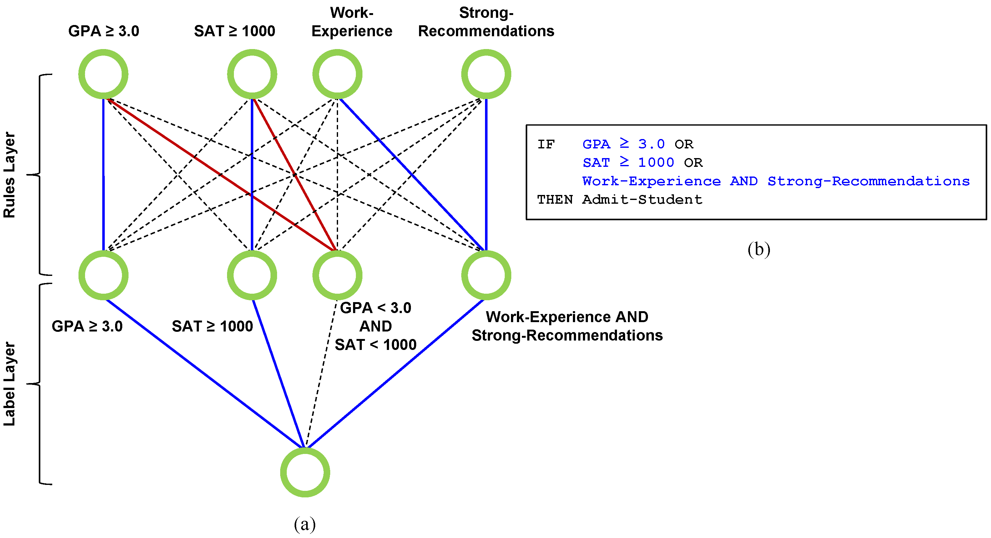
As described in [11], the decision rules network (DR-Net for short) is a simple three-layer neural network architecture, comprising an input layer of n input units, a hidden layer of k neurons, and an output layer with a single output neuron. A toy example is shown in Figure 1a for predicting college admissions, which we use to illustrate several key ideas regarding the DR-Net architecture. In this example, the first input “GPA ≥ 3.0” indicates that the student has at least a high school grade point average (GPA) of 3.0. The second input “SAT ” indicates that the student has scored at least 1000 on the SAT college entrance exam. The last two inputs indicate whether or not the student has work experience and strong letters of recommendation, respectively.
Each of the n units at the input layer pass their corresponding assigned binarized value to each neuron in the hidden layer. Denoted as the Rules Layer, the hidden layer contains k AND neurons to implement k logical-AND operations. The output unit, denoted as the Label Layer, implements a disjunction (logical OR) of the k AND neurons in the hidden layer.
In the Rules Layer shown in Figure 1a, the blue lines indicate positive weights, the red lines indicate negative weights, and the dashed lines indicate zero weights, which means the corresponding inputs are excluded from the rule formed. For example, the first hidden layer neuron is interpreted as the rule “GPA ≥ 3.0”. For the third hidden layer neuron, the red lines indicate “NOT (GPA ≥ 3.0) AND NOT (SAT ≥ 1000)”, which is equivalently represented as the rule “GPA < 3.0 AND SAT < 1000”. The last neuron is interpreted as the rule “Work Experience AND Strong Recommendations”. Similarly, in the Label Layer, the blue lines again indicate positive weights, which means the corresponding rule is included in the rule set, and the dashed lines indicate zero weights, which means the corresponding rule is excluded from the rule set. Together with the hidden layer of the AND neurons, the overall DR-Net architecture implements a trainable AND-OR network as a Boolean formula in DNF that directly maps to an unordered set of IF-THEN rules, as shown, for example, on the right-hand side of Figure 1b.
The key difference between this work and our earlier work in [11] is in the definitions of the AND and OR neurons, as described in Section 3, in that both AND and OR neurons are uniformly formulated the same way with continuous weights, which enables them to be trainable with different regularization methods, for example, the sparsity-based regularization methods described in Section 5. In addition, our OR neuron formulation is generalized to allow for the negation of inputs. As explained in Section 3, the OR neuron is generally defined so that it can include the disjunction of a binary variable or its negation , depending on whether the corresponding weight is positive or negative.
A variant of Figure 1 is shown in Figure 2. As shown in Figure 2a, a negative weight is indicated by the red line in the Label Layer, which corresponds to the negation of the corresponding rule. In Figure 2a, the AND rule for the third hidden layer neuron is “GPA < 3.0 AND SAT < 1000”. The corresponding red line to the OR output neuron means the negation of this rule. By De Morgan’s law, this negation simply rewrites the AND rule by negating each binarized feature and OR-ing them together, which means the result logic will again be in disjunctive normal form. In particular, the negation of “GPA < 3.0” is “GPA ≥ 3.0” and the negation of “SAT < 1000” is simply “SAT ≥ 1000”. Therefore, the negation of “GPA < 3.0 AND SAT < 1000” is simply “GPA ≥ 3.0 OR SAT ≥ 1000”, which results in the same set of IF-THEN rules, as shown in Figure 2b. The corresponding rule to the red line is also shown in red in the IF-THEN rules shown in Figure 2b.
4.2. NAND-NAND Network
In addition to modifying the DR-Net architecture with our formulations of AND and OR neurons, we also propose an alternative architecture of the decision rules network called the NAND-NAND network (NN-Net), which is also a three-layer fully connected neural network that translates to a decision rule set in the disjunctive normal form with the categorical and numerical attributes binarized based on the same strategy as DR-Net. In particular, the main difference between NN-Net and DR-Net is that while the Rules Layer and the Label Layer of DR-Net encode a set of logical AND operators and an OR operator, respectively, NN-Net implements two levels of NAND operators cascading together with its Rules and Label Layers.
As previously discussed, the set of decision rules in disjunctive normal form derived from DR-Net can be viewed as OR-of-ANDs, which are naturally implemented with a set of AND operators connecting to an OR operator. Mathematically, is denoted by the i-th predicate in the k-th rule, and a decision rule set is expressed as follows:
where ⋁ and ⋀ represent an AND operation and an OR operation, respectively. According to De Morgan’s laws, the negation of a disjunction is the conjunction of the negations: . As a result, the DNF in Equation (8) can be converted to two levels of conjunctions as follows:
where corresponds to a logical-NAND (NOT-AND) operation. In other words, NAND-of-NANDs is logically equivalent to OR-of-ANDs. Therefore, NN-Net has the exact same structure as DR-Net, where the hidden layer contains n hard NAND neurons and the output layer only has one soft NAND neuron.
Although formulated differently, NN-Net can be interpreted in the same way as DR-Net. That is, the hard NAND neurons in the Rules Layer of NN-Net encode rules in the same ways as the hard AND neurons in the Rules Layer of DR-Net, which will then be selected by the soft NAND neuron in the Label Layer. The equivalence of translation to the decision rule set between NN-Net and DR-Net can be explained by the following two observations: (1) negations of the outputs from the Rules Layer NAND neurons can be separated out and folded into the Label Layer, and (2) the negations of the inputs of the NAND neuron in the Label Layer are essentially performing an OR operation, according to De Morgan’s laws. The first observation shows that a set of conjunction rules can be readily translated from the weights of the Rules Layer in NN-Net just like in DR-Net, while the second one reveals that the method of interpreting the disjunction of the conjunction rules derived from the Rules Layer also involves looking at the weights of the output neuron of NN-Net. More specifically, in light of the extra negation of the inputs borrowed from the hidden layer, the NOT-NAND neuron in the Label Layer of NN-Net will output true if one of the neurons in the Label Layer has the output that matches the sign of the corresponding weight. Thus, the neuron in the Label Layer combines the rules encoded in the Rules Layer disjunctively, where the positive and negative weights require the positive and negative associations of the corresponding rules, respectively, while the zero weights discard the rules completely.
5. Simplifying Rules through Sparsity
The neural network structures we propose, DR-Net and NN-Net, specifically, provide an innovative method for the derivation of decision rule sets using the optimization technique of stochastic gradient descent. A characteristic of these networks is that zero weights in the Rules and Label Layers denote the exclusion of related input features and rules, respectively. Thus, maximizing the sparsity of the Rules and Label Layers leads to a reduction in the number of conditions in the rule set, and concurrently eliminates superfluous rules. However, an inherent challenge in the standard network training process is achieving an exact zero weight, since the widely used regularization does not explicitly penalize non-zero parameters.
To explicitly reduce the complexity of the derived rule set, the earlier work [11] only proposed one sparsity-promoting mechanism that leverages the recently proposed regularization. In this work, the new uniform definitions of AND, OR, and NAND neurons enable more versatile punning methods to be applied in our networks without any special adaption. To attain many exact zero weights, we have experimented with incorporating two sparsity-based mechanisms into the training process: (1) the recently proposed regularization that introduces trainable mask variables that are attached to all weights, and (2) the reweighted regularization [13] approach that drives the weights with small absolute values to zero by employing a log-sum penalty term.
In particular, the sparsity-promoting regularization is applied to both the Rules Layer and the Label Layer as follows:
where and are the regularization penalty terms with respect to the Rules Layer and the Label Layer, respectively, and and are the corresponding regularization coefficients that balance the classification accuracy and the rule set complexity. Intuitively, larger and will result in a lower number of conditions per rule and a lower number of rules, respectively. With the regularization techniques formulated by Equation (10) incorporated, the overall loss function we optimize for can be expressed as follows:
where is the binary cross-entropy loss.
5.1. Sparsification with Regularization
Following the regularization approach to achieve network sparsity discussed in [14], each weight is associated with a binary random variable to signify its retention or removal, thereby enabling the representation of each weight as the product of a modified weight and the corresponding binary random variable :
Assuming each follows a Bernoulli distribution with parameter that represents the probability of the being 1, i.e., , Ref. [14] uses regularization by adding all parameters to the loss function, penalizing the probabilities of masks being 1, and thus enhancing network sparsity. This regularization is readily applied to both DR-Net and NN-Net by substituting all weights with the product of the corresponding mask variables.
We denote, as and , the penalty of the non-zero mask variables of the neurons in the Rules Layer and the output neuron in the Label Layer, respectively, where is the feature index, and is the index to the j-th neuron. Then, the regularization loss in Equations (10) and (11) can be specified as follows:
5.2. Sparsification with Reweighted Regularization
Alternatively, the reweighted regularization approach proposed in [13] encourages both zero weights and weights with small absolute values. In particular, this regularization technique penalizes smaller absolute value weights so that they are driven towards zero faster, resulting in more weights at or near zero. We also incorporate a pruning method [15] to prune weights with absolute values below a certain threshold. Weights near this threshold that remain tend to be small so that they are more likely to be eliminated from the logic operations. In particular, reweighted minimization can be achieved by employing a log-sum penalty term in both layers. Therefore, the reweighted regularization loss is formulated as follows:
where and are the weights of the Rules Layer neurons and the Label Layer output neuron, respectively, and is a small value added to ensure numerical stability (e.g., ).
6. Experimental Evaluation
In this section, we evaluate DR-Net and NN-Net with both sparsity-promoting mechanisms proposed in Section 5: DR-Net with regularization (DR-Net-L0), DR-Net with reweighted regularization (DR-Net-RE), NN-Net with regularization (NN-Net-L0), and NN-Net with reweighted regularization (NN-Net-RE). Specifically, for all four variations, we show the convergence of networks in the training process, analyze the effectiveness of the sparsity-promoting mechanisms in reducing the rule set complexity, demonstrate the high predictive performances of the proposed DRNet and NNNet, and compare with other state-of-the-art rule learning methods in terms of the accuracy–complexity trade-off.
The numerical experiments were evaluated on four publicly available tabular learning datasets, all of which contain more than 10,000 training instances. The first two datasets are from the UCI Machine Learning Repository [16]: Adult Census (adult) and MAGIC Gamma Telescope (magic). These datasets have also been used in recent works on decision rule learning [5,6,17]. The remaining two datasets are the FICO HELOC dataset (heloc) [18] and the home price prediction dataset (house) [19]. As with prior works [5,6] compared in our evaluation, categorical and numerical attributes are first binarized using well-known encodings, as explained in Section 2.1.
The results of the experiments typically include test accuracies and complexities of the derived decision rule sets. Three types of complexities of the decision rule sets are considered in the experiments: number of rules, rule complexity, and model complexity, which capture different aspects of the decision rule models. We define model complexity as the number of rules plus the total number of conditions in the rule set, and rule complexity as the average number of conditions in each rule of the model.
Unless specified otherwise, both DR-Net and NN-Net were trained for 2000 epochs using the Adam optimizer with a fixed learning rate of and no weight decay across all experiments. For simplicity, the batch size was fixed at 400, the weights of Rules Layer neurons were uniformly initialized within the range of 0 to 1, and the weights of the Label Layer output neuron were initialized to all be 1. For regularization, we used the same parameters as proposed in [14]. For reweighted regularization, the pruning threshold was set as one tenth of the layer’s standard deviation, and was selected to be .
6.1. Training Analysis
We first analyzed the different behaviors of all four methods (DR-Net-L0, DR-Net-RE, NN-Net-L0, and NN-Net-RE) in the training process, and then explored the possible influences that different hyper-parameters can have over the derived decision rules. The results in this subsection were obtained by training all four methods on the adult dataset, and each network was initialized with 1000 neurons in the Rules Layer to allow sufficient modeling capability.
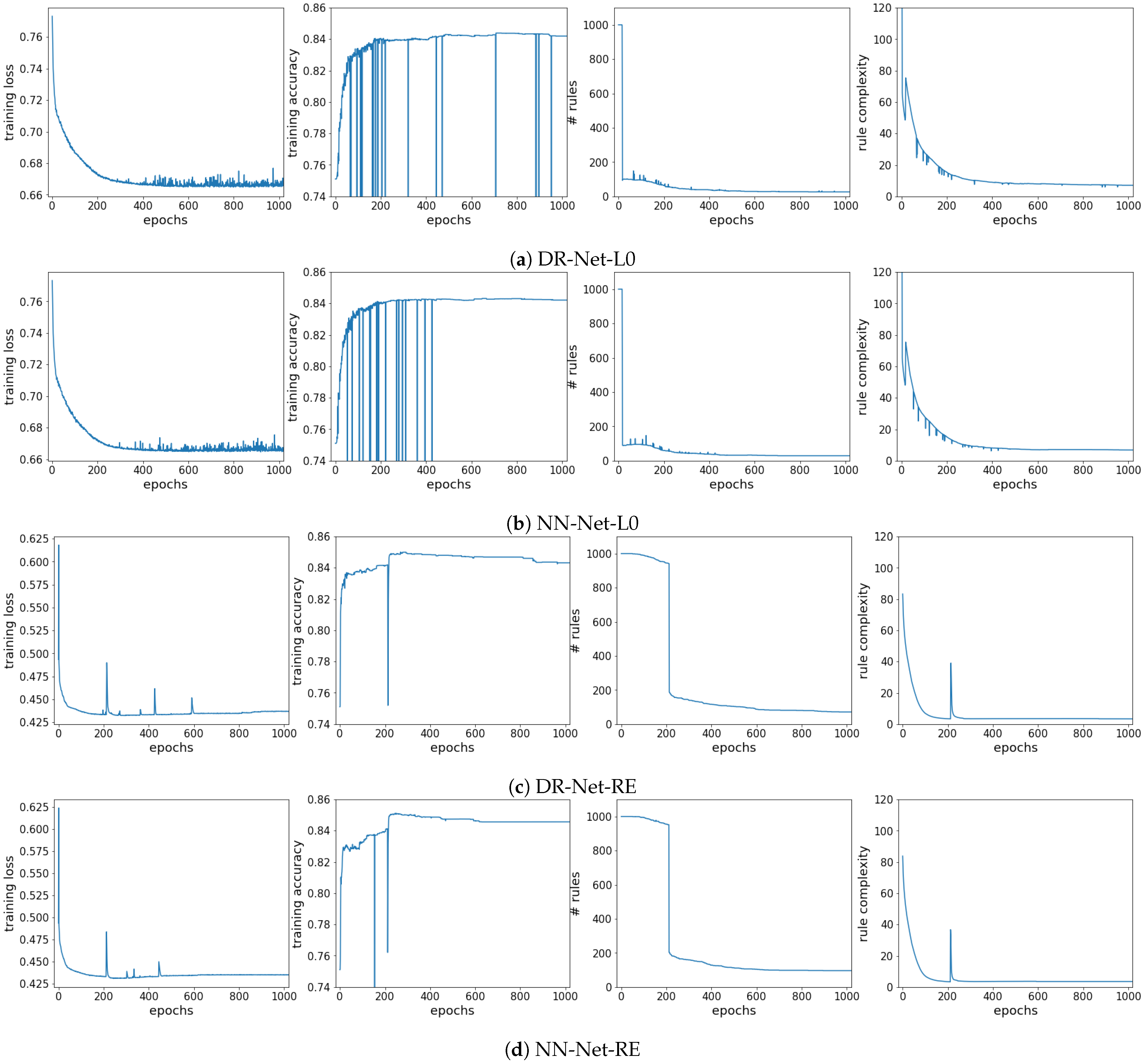
Training Convergence and Complexity Reduction. In this experiment, we empirically demonstrate that the ideas of dynamic bias and the binary step activation function with the modified straight-through estimator can work together to ensure a smooth training procedure. Figure 3 shows four statistics (training loss, training accuracy, number of rules, and rule complexity) recorded in the training processes of all four methods as functions of the training epochs, which were all trained with and on the entire adult dataset. Note that only the first half of the training procedure (first 1000 epochs) is shown in the figure, while the second half was omitted from the figures to save space, as we noticed that the four statistics for all networks were very stable after 1000 epochs.
First, we notice that DR-Net (DR-Net-L0 and DR-Net-RE) and NN-Net (NN-Net-L0 and NN-Net-RE) have very similar curves for all metrics, which experimentally proves that their architectures are interchangeable and that our neuron designs truly mimic the operations of the Boolean logic gates. The overall trends for all plots match our expectations. In particular, the training losses, the number of rules, and the rule complexities decrease with the increasing number of epochs until convergences at around epoch 400 for all methods. Furthermore, the training accuracies increase from 0.75 (all predictions are 0) to around 0.84 as the number of epochs increases.
However, there are many strong dips in the training process of the networks with regularization, where the training accuracies suddenly drop to around 0.25 and resume previous levels in the next epoch. Some minor spikes and dips are also noted in the plots of the number of rules and the plots of the rule complexity, respectively, which exactly correspond to the strong dips found in the plots of training accuracy. These spikes and dips happened in the training process because a weight in the Label Layer was trained to be negative, and thus, the corresponding rule in the Rules Layer was automatically converted to a set of rules with a single negated feature in each rule according to De Morgan’s laws, as discussed in Section 3. The conversion from the negation of a rule to a set of rules with a single feature in each rule explains the spikes in the number of rules and dips in the rule complexities. Since every instance has a very high probability of being covered by at least one of the converted rules that have the single negated feature, the networks will predict all instances to be the positive class, which results in the strong dips in the training accuracies. However, as we can see from the plots, continuing training with only one more epoch can conveniently fix the error, and thus, normally there will not be any negative weights in the Label Layer in practice if all Label Layer weights are initialized with positive weights.
Lastly, we note that the number of rules decreased dramatically in the first few epochs of the training period for DR-Net-L0 and NN-Net-L0, as most of the rules were obviously redundant and pruned simultaneously. The behavior of a significant decrease in the number of rules can also be observed for the networks trained using reweighted regularization at around epoch 200, which explains the disturbances found in the rest of the plots in Figure 3c,d.
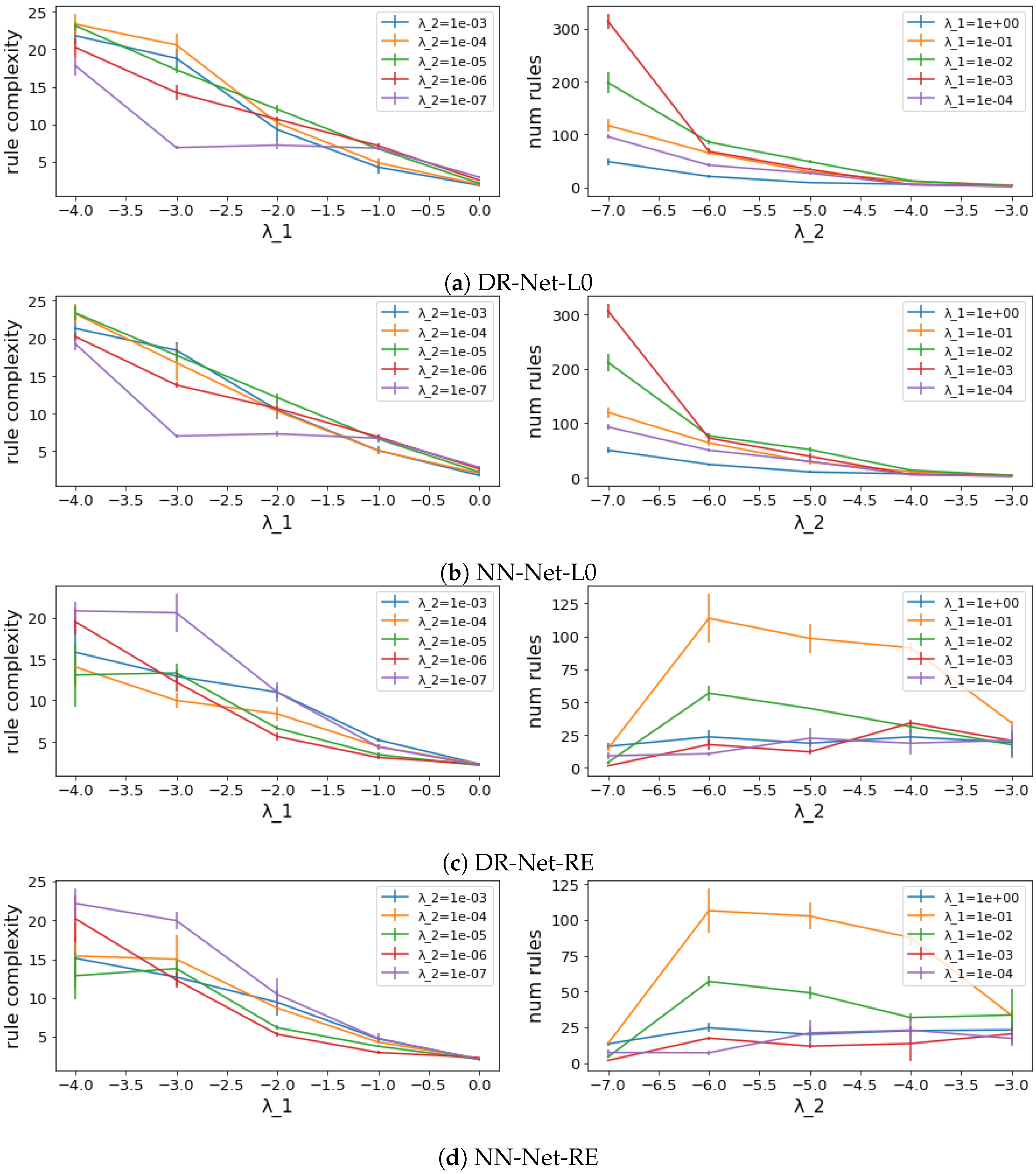
Effects of sparsity-promoting mechanisms. As discussed in Section 5, the rule set complexities can be adjusted by setting different combinations of regularization coefficients and . In theory, the regularization coefficient for the Rules Layer should affect the number of conditions per rule, which is captured by rule complexity, and the regularization coefficient for the Label Layer should influence the total number of rules. We explore, in this experiment, how effective the two proposed sparsity-promoting mechanisms are by changing the regularization coefficients and observing how the rule complexity and number of rules change, respectively. In particular, we trained all four methods with five different and five different for each method on the adult dataset using five-fold cross-validation. The average complexity values (rule complexity and number of rules) and their standard deviations for different regularization parameters ( and ) are shown in Figure 4.
In the left column of Figure 4, each line in each plot shows the changes in the rule complexity as increases for a fixed value of . For all four methods, the rule complexities monotonically decrease as increases from to 1 (note that the values on the x-axes are all on log scales), showing the high effectiveness of the regularization term for the Rules Layer among all four methods. The good correlation between the rule complexity and for all methods provides our methods with a foundation for excellent accuracy–complexity trade-off capabilities. Similarly, the lines in the right column of Figure 4 indicate how the number of rules of the derived decision rule set is changed with respect to given that is fixed for each line. The number of rules also decreases monotonically as increases from to for the networks with regularization, while there is no clear relation between the number of rules and for networks trained with reweighted regularization. Thus, compared to networks with reweighted regularization, networks trained using regularization demonstrate better potential for reducing the number of rules, as a larger will consistently result in fewer rules. However, training networks with reweighted regularization should still be considered as a valid approach, since even the maximum value of the number of rules for DR-Net-RE and NN-Net-RE shown in Figure 4 has been pruned to be less than 125, which is a substantial reduction compared to the starting point of 1000 rules.
6.2. Classification Performance and Interpretability
Next, we demonstrate the advantages of our proposed methods in terms of both predictive performance and rule set interpretability by comparing them with three other state-of-the-art rule learning algorithms: the RIPPER algorithm (RIPPER) [2], Bayesian rule set (BRS) [5], and the column generation algorithm (CG) [6]. On the other hand, BRS and CG are examples of recent works in the rule learning literature that explicitly consider the interpretability in the training process. We used open-source implementations on GitHub for all three algorithms, where the CG implementation [20] is slightly modified from the original paper.
In running the experiments comparing our methods with the decision rule set learning algorithms mentioned above, we only tuned the hyper-parameters that directly affect the interpretability of the rule sets. In particular, we varied the maximum number of conditions and the maximum number of rules, as they are provided by the implementation of RIPPER to constrain the overall complexity of the final model. For BRS, we modified the prior multiplier that affects the probability of selecting rules with different lengths, which was also used in [6]. The official implementation [20] of the column generation algorithm (CG) [6] provides two hyper-parameters to set the costs of adding a rule and a condition, and thus they, instead of the complexity bound parameter C described in the previous paper, were used in the experiments. Lastly, for DR-Net-L0, NN-Net-L0, DR-Net-RE, and NN-Net-RE, combinations of and were varied.
Maximizing Accuracy. To show the upper limits of the predictive performances of our proposed methods, we also included three traditional machine learning methods: classification and regression tree (CART) [21], random forest (RF) [8], and a deep neural network (DNN). In the experiment, we used scikit-learn [22] implementations for both CART and RF, for which the maximum depth of trees was fixed to be 100 to achieve better generalization. DNN consisted of six fully connected layers with the ReLU function as the activation function between the layers, and each hidden layer of DNN had a fixed number of 50 neurons to ensure enough learning capacity. DNN was trained with 10,000 epochs, a batch size of 2000, a learning rate of , and a weight decay of . Note that RF and DNN are typically considered as uninterpretable models, which serve as baselines and benchmarks of what black box models can achieve with the datasets.
To ensure a fair comparison among all rule learners, we leveraged five-fold nested cross-validation to select the best set of hyper-parameters for each rule learner on each dataset that maximized the validation accuracy. Also, the ranges of the hyper-parameters to be varied for each method were purposely constrained so that the learned decision rule sets were fairly interpretable to the users. Thus, for DR-Net-L0, DR-Net-RE, NN-Net-L0, and NN-Net-RE, the number of neurons in the Rules Layer was chosen to be only 50. The test accuracy results of all models on all datasets are shown in Table 1. Note that all results in Table 1 for CG, BRS, RIPPER, CART, RF, and DNN are copied from [11].
It can be seen in Table 1 that across all datasets, all variants of DR-Net and NN-Net outperform other interpretable models in terms of the testing accuracy in most cases, with few exceptions. The method with the overall best testing accuracy (NN-Net-L0) can achieve a very similar predictive performance compared to uninterpretable models (RF and DNN), with only a 3% discrepancy. As expected, there is no noticeable difference between the variants of DR-Net and NN-Net in terms of the accuracies, since their architectures are essentially established based on the same logic operations. The results in Table 1 suggest that our proposed methods are very competitive as a machine learning model for interpretable classification.
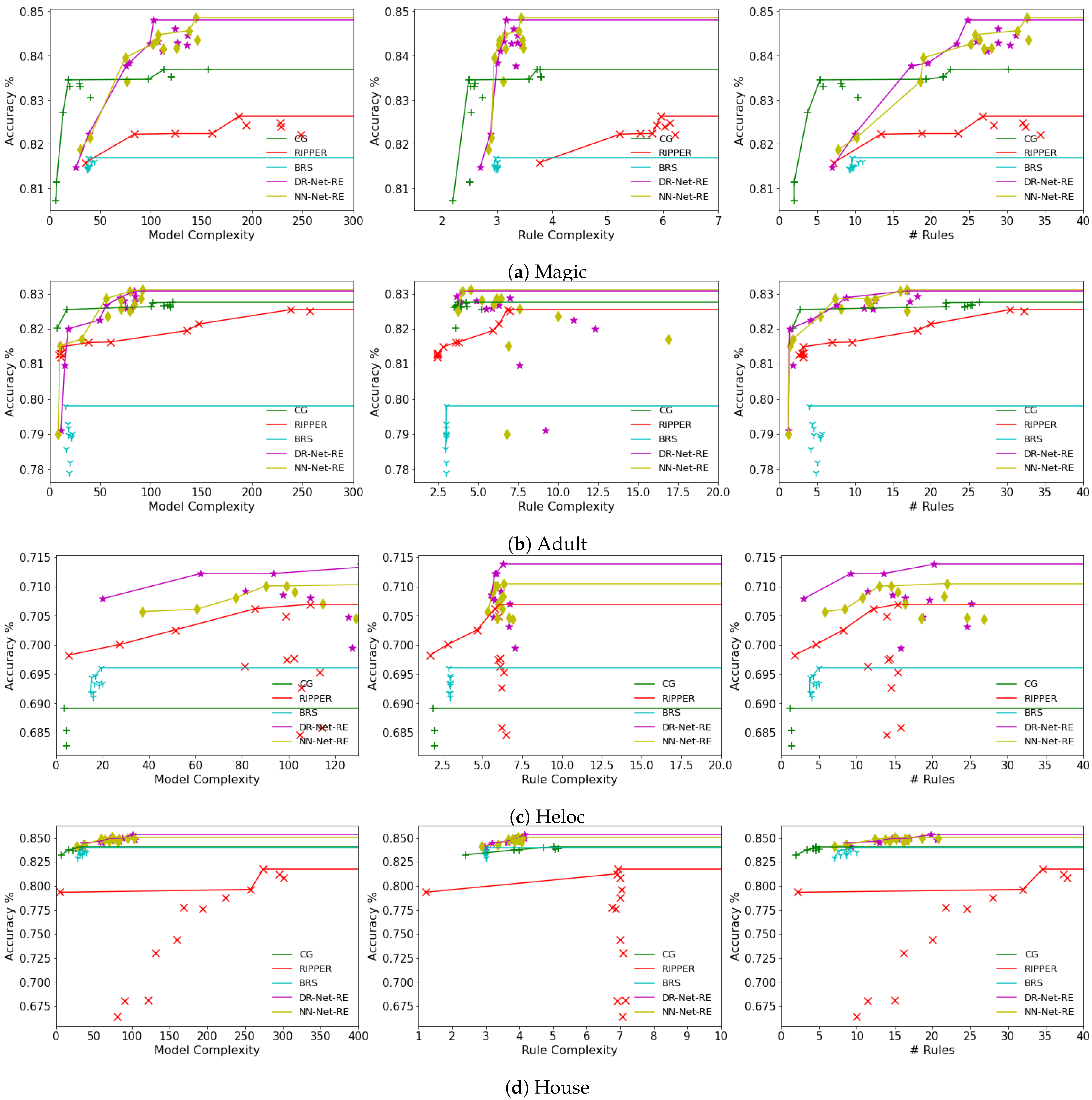
Accuracy–complexity trade-off. Finally, the accuracy–complexity trade-off abilities were evaluated among all decision rule learning methods, which included DR-Net-L0, DR-Net-RE, NN-Net-L0, NN-Net-RE, RIPPER, BRS, and CG. Different sets of accuracy–complexity pairs were generated for each method on each dataset by running the algorithm with a wide range of hyper-parameter values. We ran the experiments on all datasets, and the results, along with the average of the five-fold cross-validation, are shown in Figure 5 and Figure 6. For each method compared, the dots connected by the line segments shown correspond to Pareto efficient models, where all other points below the Pareto frontier have either lower accuracies or higher complexities. Again, all results in Figure 5 and Figure 6 for CG, BRS, and RIPPER are from [11].
The defining attribute of both DR-Net and NN-Net, namely, the ability to reach high test accuracy while maintaining an acceptable level of model complexity, is further emphasized in Figure 5 and Figure 6. For both the heloc and house datasets, it becomes apparent that all variants of DR-Net and NN-Net outperform other rule learners across all three complexity metrics. This superiority is demonstrated by the fact that their Pareto efficient points consistently occupy the top positions. With regard to the magic and adult datasets, all variations of DR-Net and NN-Net continue to showcase superior performance over other rule learners in terms of accuracy, and this margin of superiority becomes substantially evident when the model complexity, rule complexity, or the number of rules surpasses a specific threshold. BRS, on the other hand, fails to present a clear accuracy–complexity trade-off, as its results are tightly clustered within a narrow range, an observation that has been noted and explained in [6,11]. This experiment affirms the potential advantages of DR-Net and NN-Net over other rule learners, primarily due to their capability of achieving a significantly higher test accuracy with a relatively moderate sacrifice in complexity.
7. Related Work
Decision rule learning has been extensively studied in the literature, most of which employs heuristic algorithms, but earlier methods optimize for criteria that are not necessarily directly related to classification accuracy or model simplicity. Examples include association rule mining and classification [23,24], logical analysis methods [25,26,27], and greedy set covering approaches [2].
Recently, researchers have improved on decision rule learning algorithms by explicitly considering the interpretability of rules in designing algorithms. In particular, one solution of incorporating interpretability is to add model complexity to the optimization objective so that simplicity can be jointly optimized together with prediction accuracy. Some methods in this category select rules from a set of candidate rules, and thus, a rule-mining algorithm is employed in the preprocessing step for these methods. Examples include a Bayesian framework that is approximately solved using simulated annealing [5] and an optimization problem solved by a local search algorithm [4]. However, the requirement of starting with pre-mined rules limits the overall search space and their ability to find a globally optimized solution.
There are other methods based on integer programming (IP) formulations that do not require pre-mining of the rules, but only approximate solutions can be found for large datasets due to the inherent complex nature of the problems. For example, in [6], the IP problem is approximately solved by relaxing it into a linear programming problem and applying the column generation algorithm. In [3], various optimization approaches are utilized, including block coordinate descent and alternating minimization algorithm.
In addition to decision rule sets, decision lists [28,29,30] and decision trees [21,31] are also explainable rule-based models. Decision lists capture rules in an ordered IF-THEN-ELSE sequence. However, the cascading of rules in an IF-THEN-ELSE sequence means that the interpretation of an activated rule will unfortunately require an understanding of all preceding rules, which makes the explanation more difficult for humans to understand. Decision trees implicitly organize rules into a tree structure, corresponding to paths in the tree. However, these rules are typically more complex, and thus, decision trees are often prone to overfitting.
Building on the notable success that deep neural networks have had on perceptual learning tasks like image classification, researchers have also recently turned to neural network models for tabular data learning [9,10,32,33]. The works in [9,10] aimed to capture the aspects of gradient boosting decision trees and random forests that have made these models successful, and they were able to achieve comparable performance using these approaches with neural models. However, like gradient boosting decision trees and random decision forests, these models are also uninterpretable in the sense that they do not provide explanations that are easily understandable by humans. On the other hand, the works in [32,33] are designed to be explainable.
8. Conclusions
In this paper, we extended recent work on decision rule learning based on neural net architectures that can be accurately trained for tabular data classification. In particular, we presented alternative formulations to trainable Boolean logic operators as neurons with continuous weights, including trainable NAND neurons. These alternative formulations provide uniform treatments to different trainable logic neurons so that they can be trained the same way. This enables, for example, the direct application of existing sparsity-promoting neural net training techniques like reweighted regularization to derive sparse networks that translate to simpler decision rule sets, in addition to a stochastic regularization approach that was previously used in [11]. Further, we presented an alternative network architecture based on trainable NAND neurons by applying De Morgan’s law to realize a NAND-NAND network instead of an AND-OR network. Our experimental results show that these alternative formulations can also generate accurate decision rule sets that achieve state-of-the-art performance in terms of accuracy in tabular learning applications.
Furthermore, since all our proposed AND, OR, and NAND neurons are now uniformly defined, layers of different neurons can be freely concatenated using a different order than the ones proposed in this paper. For example, a neural network that directly translates to a Conjunctive Normal Form classifier can be easily formulated by concatenating a layer of OR neurons with an output AND neuron. It would be an interesting direction of future research to see whether different layers of logical neurons can be combined in more complicated ways to achieve better predictive performances while maintaining good interpretability.
Author Contributions
Conceptualization, B.L.; methodology, L.Q. and W.W.; software, L.Q.; validation, L.Q.; formal analysis, W.W.; investigation, L.Q.; resources, L.Q.; data curation, L.Q.; writing—original draft preparation, L.Q. and W.W.; writing—review and editing, B.L.; visualization, L.Q.; supervision, B.L.; project administration, B.L.; funding acquisition, B.L. All authors have read and agreed to the published version of the manuscript.
Funding
This research has been supported, in part, by the National Science Foundation (NSF IIS-1956339).
Conflicts of Interest
The authors declare no conflict of interest.
References
- Rudin, C. Stop Explaining Black Box Machine Learning Models for High Stakes Decisions and Use Interpretable Models Instead. Nat. Mach. Intell. 2019, 1, 206–215. [Google Scholar] [CrossRef]
- Cohen, W.W. Fast Effective Rule Induction. In Proceedings of the Twelfth International Conference on Machine Learning, Tahoe City, CA, USA, 9–12 July 1995; Morgan Kaufmann: Burlington, MA, USA, 1995; pp. 115–123. [Google Scholar]
- Su, G.; Wei, D.; Varshney, K.R.; Malioutov, D.M. Interpretable Two-level Boolean Rule Learning for Classification. arXiv 2015, arXiv:1511.07361. [Google Scholar]
- Lakkaraju, H.; Bach, S.H.; Leskovec, J. Interpretable Decision Sets: A Joint Framework for Description and Prediction. In Proceedings of the 22nd ACM SIGKDD International Conference on Knowledge Discovery and Data Mining (KDD ’16), New York, NY, USA, 13–17 August 2016; pp. 1675–1684. [Google Scholar] [CrossRef] [Green Version]
- Wang, T.; Rudin, C.; Doshi-Velez, F.; Liu, Y.; Klampfl, E.; MacNeille, P. A Bayesian Framework for Learning Rule Sets for Interpretable Classification. J. Mach. Learn. Res. 2017, 18, 1–37. [Google Scholar]
- Dash, S.; Günlük, O.; Wei, D. Boolean Decision Rules via Column Generation. In Proceedings of the 32nd International Conference on Neural Information Processing Systems (NIPS’18), Red Hook, NY, USA, 13–18 December 2018; pp. 4660–4670. [Google Scholar]
- Chen, T.; Guestrin, C. Xgboost: A scalable tree boosting system. In Proceedings of the 22nd ACM Sigkdd International Conference on Knowledge Discovery and Data Mining, San Francisco, CA, USA, 13–17 August 2016; pp. 785–794. [Google Scholar]
- Breiman, L. Random Forests. Mach. Learn. 2001, 45, 5–32. [Google Scholar] [CrossRef] [Green Version]
- Arık, S.O.; Pfister, T. Tabnet: Attentive interpretable tabular learning. In Proceedings of the AAAI Conference on Artificial Intelligence, New York, NY, USA, 7–12 February 2020. [Google Scholar]
- Katzir, L.; Elidan, G.; El-Yaniv, R. Net-DNF: Effective Deep Modeling of Tabular Data. In Proceedings of the International Conference on Learning Representations, Addis Ababa, Ethiopia, 26–30 April 2020. [Google Scholar]
- Qiao, L.; Wang, W.; Lin, B. Learning Accurate and Interpretable Decision Rule Sets from Neural Networks. In Proceedings of the AAAI, Virtually, 2–9 February 2021. [Google Scholar]
- Bengio, Y.; Léonard, N.; Courville, A. Estimating or Propagating Gradients through Stochastic Neurons for Conditional Computation. arXiv 2013, arXiv:1308.3432. [Google Scholar]
- Candès, E.; Wakin, M.; Boyd, S.P. Enhancing Sparsity by Reweighted L1 Minimization. J. Fourier Anal. Appl. 2007, 14, 877–905. [Google Scholar] [CrossRef]
- Louizos, C.; Welling, M.; Kingma, D.P. Learning Sparse Neural Networks through L0 Regularization. arXiv 2017, arXiv:1712.01312. [Google Scholar]
- Han, S.; Pool, J.; Tran, J.; Dally, W. Learning both Weights and Connections for Efficient Neural Network. arXiv 2015, arXiv:1506.02626. [Google Scholar]
- Dua, D.; Graff, C. UCI Machine Learning Repository. 2017. Available online: http://archive.ics.uci.edu/ml (accessed on 25 June 2023).
- Dash, S.; Malioutov, D.M.; Varshney, K.R. Screening for learning classification rules via Boolean compressed sensing. In Proceedings of the 2014 IEEE International Conference on Acoustics, Speech and Signal Processing (ICASSP), Florence, Italy, 4–9 May 2014; pp. 3360–3364. [Google Scholar]
- Chen, C.; Lin, K.; Rudin, C.; Shaposhnik, Y.; Wang, S.; Wang, T. An Interpretable Model with Globally Consistent Explanations for Credit Risk. arXiv 2018, arXiv:1811.12615. [Google Scholar]
- Vanschoren, J.; van Rijn, J.N.; Bischl, B.; Torgo, L. OpenML: Networked Science in Machine Learning. SIGKDD Explor. 2013, 15, 49–60. [Google Scholar] [CrossRef] [Green Version]
- Arya, V.; Bellamy, R.K.E.; Chen, P.Y.; Dhurandhar, A.; Hind, M.; Hoffman, S.C.; Houde, S.; Liao, Q.V.; Luss, R.; Mojsilović, A.; et al. One Explanation Does Not Fit All: A Toolkit and Taxonomy of AI Explainability Techniques. arXiv 2019, arXiv:1909.03012. [Google Scholar]
- Breiman, L.; Friedman, J.; Stone, C.; Olshen, R. Classification and Regression Trees; The Wadsworth and Brooks-Cole Statistics-Probability Series; Taylor & Francis: Abingdon, UK, 1984. [Google Scholar]
- Pedregosa, F.; Varoquaux, G.; Gramfort, A.; Michel, V.; Thirion, B.; Grisel, O.; Blondel, M.; Prettenhofer, P.; Weiss, R.; Dubourg, V.; et al. Scikit-learn: Machine Learning in Python. J. Mach. Learn. Res. 2011, 12, 2825–2830. [Google Scholar]
- Clark, P.; Niblett, T. The CN2 Induction Algorithm. Mach. Learn. 1989, 3, 261–283. [Google Scholar] [CrossRef]
- Liu, B.; Hsu, W.; Ma, Y. Integrating Classification and Association Rule Mining. In Proceedings of the Fourth International Conference on Knowledge Discovery and Data Mining (KDD’98), New York, NY, USA, 27–31 August 1998; pp. 80–86. [Google Scholar]
- Crama, Y.; Hammer, P.L.; Ibaraki, T. Cause-Effect Relationships and Partially Defined Boolean Functions. Ann. Oper. Res. 1988, 16, 299–325. [Google Scholar] [CrossRef] [Green Version]
- Boros, E.; Hammer, P.L.; Ibaraki, T.; Kogan, A.; Mayoraz, E.; Muchnik, I. An implementation of logical analysis of data. IEEE Trans. Knowl. Data Eng. 2000, 12, 292–306. [Google Scholar] [CrossRef] [Green Version]
- Qiao, L.; Wang, W.; Dasgupta, S.; Lin, B. Rethinking Logic Minimization for Tabular Machine Learning. IEEE Trans. Artif. Intell. 2022, 1–12. [Google Scholar] [CrossRef]
- Rivest, R.L. Learning Decision Lists. Mach. Learn. 1987, 2, 229–246. [Google Scholar] [CrossRef] [Green Version]
- Bertsimas, D.; Chang, A.; Rudin, C. ORC: Ordered Rules for Classification a Discrete Optimization Approach to Associative Classification; Massachusetts Institute of Technology, Operations Research Center: Cambridge, MA, USA, 2012. [Google Scholar]
- Letham, B.; Rudin, C.; McCormick, T.H.; Madigan, D. Interpretable classifiers using rules and Bayesian analysis: Building a better stroke prediction model. arXiv 2015, arXiv:1511.01644. [Google Scholar] [CrossRef]
- Rokach, L.; Maimon, O. Top–Down Induction of Decision Trees Classifiers—A survey. IEEE Trans. Syst. Man Cybern. Part C Appl. Rev. 2005, 35, 476–487. [Google Scholar] [CrossRef] [Green Version]
- Wang, W.; Qiao, L.; Lin, B. Disjunctive Threshold Networks for Tabular Data Classification. IEEE Open J. Comput. Soc. 2023, 4, 185–194. [Google Scholar] [CrossRef]
- Wang, W.; Qiao, L.; Lin, B. Tabular machine learning using conjunctive threshold neural networks. Mach. Learn. Appl. 2022, 10, 100429. [Google Scholar] [CrossRef]
Figure 1.
(a) An example of the DR-Net architecture with 4 AND neurons is shown. The blue lines to the AND neurons represent positive weights, while red lines represent negative weights. The dashed line indicates the exclusion of the corresponding input feature. Please note that we represent “NOT (GPA ≥ 3.0)” as “GPA < 3.0” in the third rule. Similarly, “NOT (SAT ≥ 1000)” is represented as “SAT < 1000”. For the output OR neuron, the blue line indicates that the corresponding rule is included in the rule set, and the dashed line indicates that the corresponding rule is excluded. (b) The network maps directly to the corresponding decision rule set shown in the box on the right.

Figure 2.
(a) A variation of the example in Figure 1, in which the red line to the output OR neuron indicates the negation of the corresponding rule “GPA < 3.0 AND SAT < 1000.” By De Morgan’s law, the negation of “GPA < 3.0 AND SAT < 1000” becomes “GPA ≥ 3.0 OR SAT ≥ 1000”, which results in the same decision rule set. (b) The corresponding decision rule set is shown on the right.

Figure 3.
Training statistics (training loss, training accuracy, number of rules, and rule complexity) as functions of the number of epochs in the training process.
Figure 3.
Training statistics (training loss, training accuracy, number of rules, and rule complexity) as functions of the number of epochs in the training process.

Figure 4.
The relations between complexities (rule complexity and number of rules) and regularization parameters ( and ). All x-axes are on a log10 scale. All complexity values were averaged over five cross-validation partitions, and the vertical bars represent standard deviations.
Figure 4.
The relations between complexities (rule complexity and number of rules) and regularization parameters ( and ). All x-axes are on a log10 scale. All complexity values were averaged over five cross-validation partitions, and the vertical bars represent standard deviations.

Figure 5.
Accuracy–Complexity trade-offs on all datasets for DR-Net and NN-Net trained using regularization. Pareto efficient points are connected by line segments.
Figure 5.
Accuracy–Complexity trade-offs on all datasets for DR-Net and NN-Net trained using regularization. Pareto efficient points are connected by line segments.

Figure 6.
Accuracy–Complexity trade-offs on all datasets for DR-Net and NN-Net trained using reweighted regularization. Pareto efficient points are connected by line segments.
Figure 6.
Accuracy–Complexity trade-offs on all datasets for DR-Net and NN-Net trained using reweighted regularization. Pareto efficient points are connected by line segments.


Table 1.
Test accuracy based on the nested five-fold cross-validation (%, standard error in parentheses).
Table 1.
Test accuracy based on the nested five-fold cross-validation (%, standard error in parentheses).
| Dataset | Magic | Adult | Heloc | House |
|---|---|---|---|---|
| Interpretable | ||||
| NN-Net-RE | 84.14 | 82.59 | 70.76 | 84.89 |
| (0.69) | (0.23) | (0.66) | (0.46) | |
| NN-Net-L0 | 84.45 | 83.13 | 70.71 | 86.17 |
| (0.51) | (0.59) | (0.67) | (0.50) | |
| DR-Net-RE | 84.63 | 82.50 | 71.05 | 84.84 |
| (0.53) | (0.68) | (0.57) | (0.66) | |
| DR-Net-L0 | 84.10 | 83.09 | 70.07 | 85.90 |
| (0.82) | (0.51) | (0.89) | (0.50) | |
| DR-Net | 84.42 | 82.97 | 69.71 | 85.71 |
| (0.53) | (0.51) | (1.05) | (0.40) | |
| CG | 83.68 | 82.67 | 68.65 | 83.90 |
| (0.87) | (0.48) | (3.48) | (0.18) | |
| BRS | 81.44 | 79.35 | 69.42 | 83.04 |
| (0.61) | (1.78) | (3.72) | (0.11) | |
| RIPPER | 82.22 | 81.67 | 69.67 | 82.47 |
| (0.51) | (1.05) | (2.09) | (1.84) | |
| CART | 80.56 | 78.87 | 60.61 | 82.37 |
| (0.86) | (0.12) | (2.83) | (0.29) | |
| Uninterpretable | ||||
| RF | 86.47 | 82.64 | 70.30 | 88.70 |
| (0.54) | (0.49) | (3.70) | (0.28) | |
| DNN | 87.07 | 84.33 | 70.64 | 88.84 |
| (0.71) | (0.42) | (3.37) | (0.26) | |
Disclaimer/Publisher’s Note: The statements, opinions and data contained in all publications are solely those of the individual author(s) and contributor(s) and not of MDPI and/or the editor(s). MDPI and/or the editor(s) disclaim responsibility for any injury to people or property resulting from any ideas, methods, instructions or products referred to in the content. |
© 2023 by the authors. Licensee MDPI, Basel, Switzerland. This article is an open access article distributed under the terms and conditions of the Creative Commons Attribution (CC BY) license (https://creativecommons.org/licenses/by/4.0/).
Share and Cite
MDPI and ACS Style
Qiao, L.; Wang, W.; Lin, B. Alternative Formulations of Decision Rule Learning from Neural Networks. Mach. Learn. Knowl. Extr. 2023, 5, 937-956. https://0-doi-org.brum.beds.ac.uk/10.3390/make5030049
AMA Style
Qiao L, Wang W, Lin B. Alternative Formulations of Decision Rule Learning from Neural Networks. Machine Learning and Knowledge Extraction. 2023; 5(3):937-956. https://0-doi-org.brum.beds.ac.uk/10.3390/make5030049
Chicago/Turabian StyleQiao, Litao, Weijia Wang, and Bill Lin. 2023. "Alternative Formulations of Decision Rule Learning from Neural Networks" Machine Learning and Knowledge Extraction 5, no. 3: 937-956. https://0-doi-org.brum.beds.ac.uk/10.3390/make5030049