A Top-to-Bottom Luminescence-Based Chronology for the Post-LGM Regression of a Great Basin Pluvial Lake


1
Geology Department, Middlebury College, Middlebury, VT 05753, USA
2
Department of Earth Sciences, Dartmouth College, Hanover, NH 03755, USA
*
Author to whom correspondence should be addressed.
Quaternary 2020, 3(2), 11; https://0-doi-org.brum.beds.ac.uk/10.3390/quat3020011
Submission received: 13 February 2020
/
Revised: 13 March 2020
/
Accepted: 9 April 2020
/
Published: 16 April 2020
Abstract
:We applied luminescence dating to a suite of shorelines constructed by pluvial Lake Clover in northeastern Nevada, USA during the last glacial cycle. At its maximum extent, the lake covered 740 km2 with a mean depth of 16 m and a water volume of 13 km3. In the north-central sector of the lake basin, 10 obvious beach ridges extend from the highstand to the lowest shoreline over a horizontal distance of ~1.5 km, representing a lake area decrease of 35%. These ridges are primarily composed of sandy gravel and rise ~1.0 m above the alluvial fan surface on which they are superposed. Single grain luminescence dating of K-feldspar using the pIRIR SAR (post-infrared infrared single-aliquot regenerative dose) protocol, corroborated by SAR dating of quartz, indicates that the highstand shoreline was constructed ca. 16–17 ka during Heinrich Stadial I (Greenland Stadial 2, GS-2), matching 14C age control for this shoreline elsewhere in the basin. The lake regressed rapidly during the Bølling/Allerød (GI-1), before the rate of regression slowed during the Younger Dryas interval (GS-1). The lowest shoreline was constructed ca. 10 ka. Persistence of Lake Clover into the early Holocene may reflect enhanced monsoonal precipitation driven by the summer insolation maximum.

1. Introduction
The pluvial lakes that existed in and around the Great Basin at times during the Pleistocene are the most iconic evidence for the profound hydroclimate shifts that accompanied glacial-deglacial cycles in southwestern North America. Fresh surface water is ephemeral or completely absent across most of this region today, owing to aridity in the rain shadow of the Sierra Nevada [1]. However, many valleys contain linear ridges of water-washed gravel that are obviously beaches and storm berms produced by waves on former lakes of significant areal extent (>500 km2) [2]. The rather remarkable realization that this dry landscape was once much wetter has motivated more than a century of research into the former size and distribution of these pluvial lakes [3,4], and considerable work over the past several decades has applied a variety of absolute dating methods to determine when these lakes reached their maximum dimensions [5,6]. These efforts have led to comprehensive catalogs of pluvial lake distribution [7], and sometimes conflicting theories about the climatic controls on these lake highstands [8,9,10,11,12].
In contrast, relatively less attention has been focused on shorelines built by these lakes at elevations below their highest levels, shorelines that were constructed when lakes were in equilibrium with reduced effective moisture relative to the highstand climate. Some of these features may have been built during lake level rise and subsequently submerged by later higher water [13]. However, for particularly well-preserved and/or small shorelines, it is geomorphically more likely that they were built during regression and lake level fall. Either way, these features contain potentially significant evidence about paleoclimate during times of transition. By way of analogy, ignoring these lower shorelines and focusing solely on the highstand ridge is similar to building a glacial chronology by dating just the terminal moraine in a glaciated valley and overlooking recessional moraines.
This study developed a top-to-bottom chronology for the entire suite of shorelines constructed by a former pluvial lake. In the course of an extensive campaign of field mapping combined with interpretation of aerial imagery, all preserved shorelines of this lake were identified and mapped. A location was selected where these shorelines are well preserved in close proximity to one another; each was then studied in the field, and sampled for luminescence dating. The resulting chronology provides a detailed perspective on the timing of changes in the extent of this lake during and after the pluvial maximum, and serves as an important point of comparison for other regional hydroclimate records spanning the last glacial-interglacial transition.
2. Materials and Methods
2.1. Setting
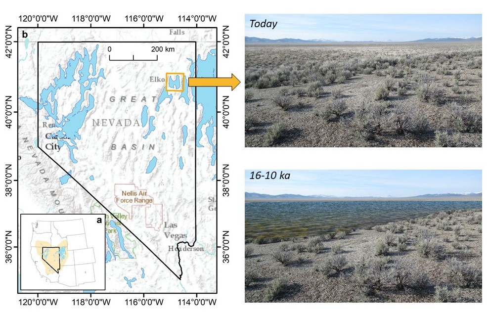
The study area for this project is the Clover and Independence Valleys of northeastern Nevada, USA (Figure 1). Small areas of ephemeral water are seasonally present on the floors of these valleys, but for the most part, the landscape is characterized by an arid expanse of sagebrush grading toward dunes and unvegetated playa surfaces at the lowest elevations. In contrast, laterally extensive beach ridges around the perimeter of the valley bottom evidence strikingly different conditions in the late Pleistocene, when Lake Clover inundated the adjacent valleys with water up to 20 m deep (Figure 1).
Lake Clover existed in a watershed that spans 1460 km2 with an elevation range of 1703 to 3419 m. A weather monitoring site near the highstand elevation of the lake (National Weather Service cooperative site 261740) has a continental climate with a mean annual temperature of 7.5 °C and a mean annual precipitation of 350 mm. Mean monthly temperatures peak in July (29.7 °C) and August (29.1 °C), and are lowest in December (3.6 °C) and January (2.6 °C). July and August are both very dry, averaging <16 mm of precipitation. January has the greatest average precipitation (45 mm), followed closely by November, December, and February (~38 mm). Conditions are colder and wetter at higher elevation. Interpolated 30-year normals from the PRISM database suggest that the mountains surrounding the Lake Clover watershed receive up to 1160 mm of precipitation per year with mean temperatures between 1 and 2 °C <http://www.prism.oregonstate.edu/>.
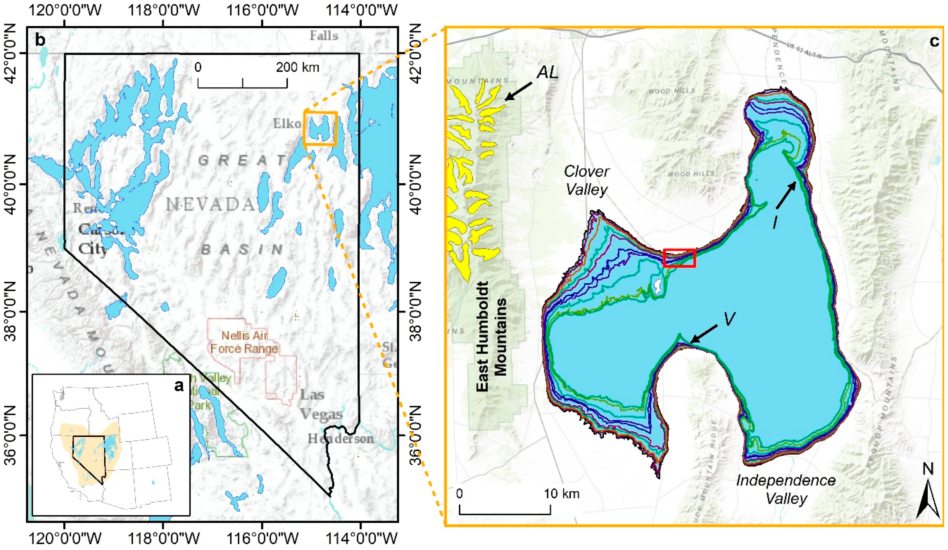
Lake Clover was selected for this project for several reasons. First, a modest number of preexisting 14C ages provided preliminary age control for the lake highstand [14]. Second, Lake Clover filled the valley immediately east of the East Humboldt Mountains (Figure 1c), where the type locality for the local Last Glacial Maximum (l-LGM) in the Great Basin, the “Angel Lake Glaciation” is located [15]. This setting provides, therefore, an unusual opportunity to simultaneously consider co-located, high-resolution pluvial and glacial records spanning the last deglaciation. Third, high-resolution records of post-glacial environmental change have been developed from lakes in the mountains immediately west of Lake Clover, providing a useful point of reference for paleoclimate changes during the last glacial-interglacial transition [16]. Finally, recent work has inferred the existence of a prominent dipole pattern in winter precipitation in this area during the late Pleistocene, with pluvial lakes in the latitude band ~39–41° N reaching their highstands ~2 ka earlier and out of phase with Lake Chewaucan farther north in Oregon [9]. A robust chronology for the highstand and regression of Lake Clover, located at 40.8° N, would provide an important test for this hypothesis.
2.2. Field Methods
Field reconnaissance in combination with interpretation of aerial imagery identified a location (40.876° N, 114.850° W) in the north-central part of the area covered by Lake Clover where the entire sequence of shorelines, from the highstand to the lowest preserved ridge, are present in close proximity to one another (Figure 1c and Figure 2). This location is bisected from WNW to ESE by the Union Pacific railroad line; a jeep trail paralleling the railroad eastward from the “Tobar” road intersection (USGS Ventosa 7.5′ quadrangle) provided access to the field site, which was referred to as the “Tobar transect”. Fieldwork was conducted at the Tobar transect in August, 2018, and again in June and August, 2019.
To quantify the dimensions and elevations of the preserved shorelines, a Topcon GTS-235W laser total station was set up on an artificial height of land along a roadcut where the railroad breaches several of the closely spaced beach ridges. The location of the total station was referenced to a second class 0 vertical order survey marker (LQ0282) located 65 m away along the railroad line. This marker was installed by the Coast & Geodetic Survey in 1934, and has a vertical error of ±5.6 cm. Two separate transects were measured (Figure 2), each taking advantage of jeep trails that provided a linear route through the sagebrush. One of these crosses shorelines north of the railroad, while the other crosses shorelines on the south side. To provide consistency in data spacing, the survey transects were marked with flagging at an interval of 6 m and measurements were made with the total station at each of these premarked points. Data were exported as xyz coordinates relative to the total station, and processed to yield a complete topographic cross section encompassing all of the shorelines in the Tobar transect.
In concert with the surveying, pits with dimensions of ~1 × 1 m were excavated by hand to a depth of ~100 cm in the crest of each shoreline (Figure 2). Locations were selected where the shoreline crest was broad and flat, where no signs of disturbance were present, and where sufficient space existed between the sagebrush to permit excavation. One shoreline was studied in a natural exposure along a gully paralleling the railroad where it is elevated on an artificial causeway. To better understand the conditions under which these shoreline berms were constructed and the sediments comprising them, the stratigraphy revealed in each exposure was measured, described, and photographed, and the soil profile (including horizon thickness, Munsell color, texture, and structure) recorded.
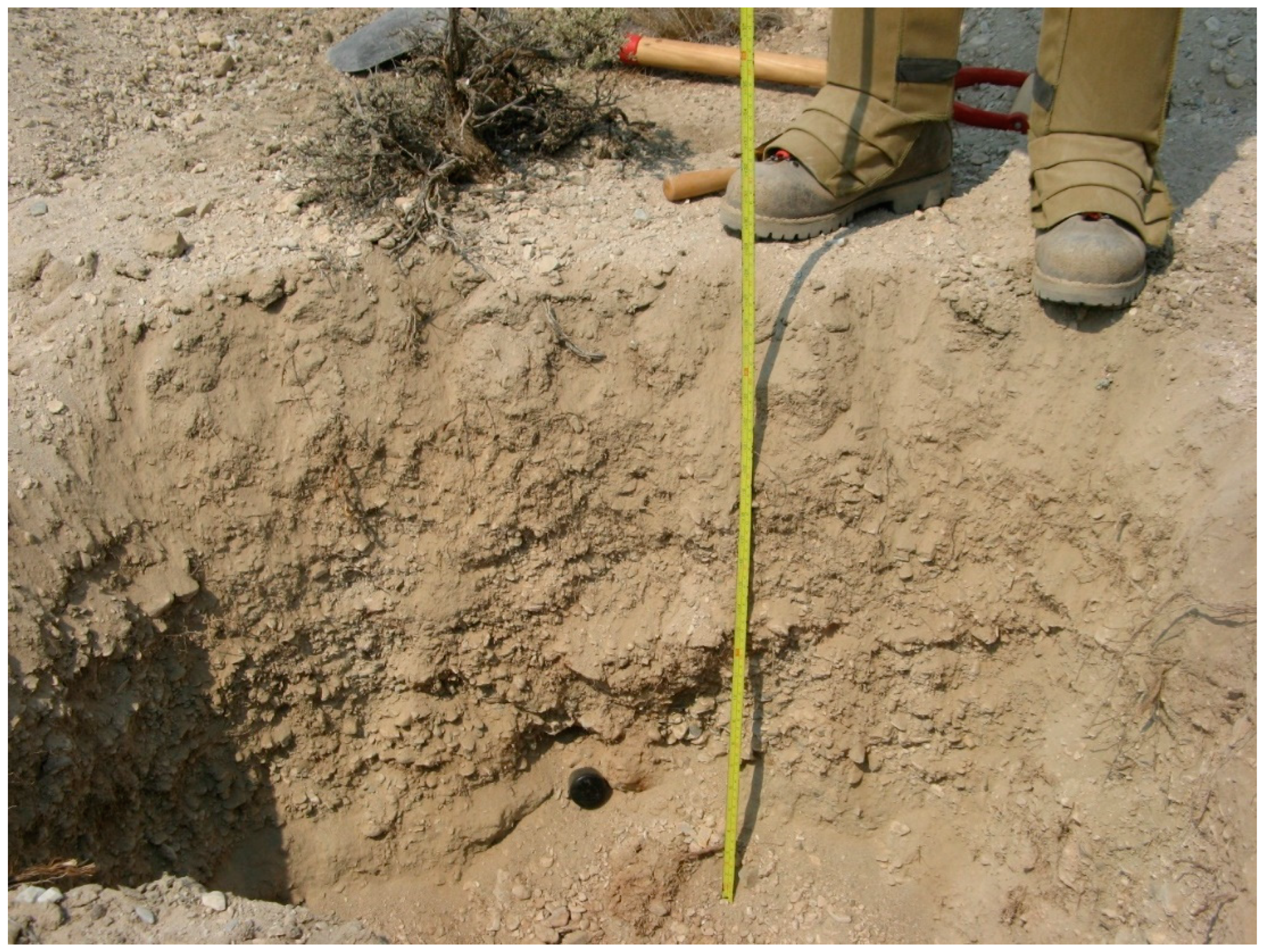
Light-shielded samples for luminescence dating were collected from sand-rich layers as deep as possible in each of these exposures by hammering a 2.5-cm-diameter, 25-cm-long metal tube into the freshly excavated pit face (Figure 3). After over-penetrating to ensure that the tube was full, tubes were excavated and immediately capped with light-proof caps secured by tape. Sediment in a ~25-cm radius around each tube was collected as the tubes were removed for the calculation of the luminescence dose rate and sediment water content in the laboratory.
2.3. Shoreline Interpretation
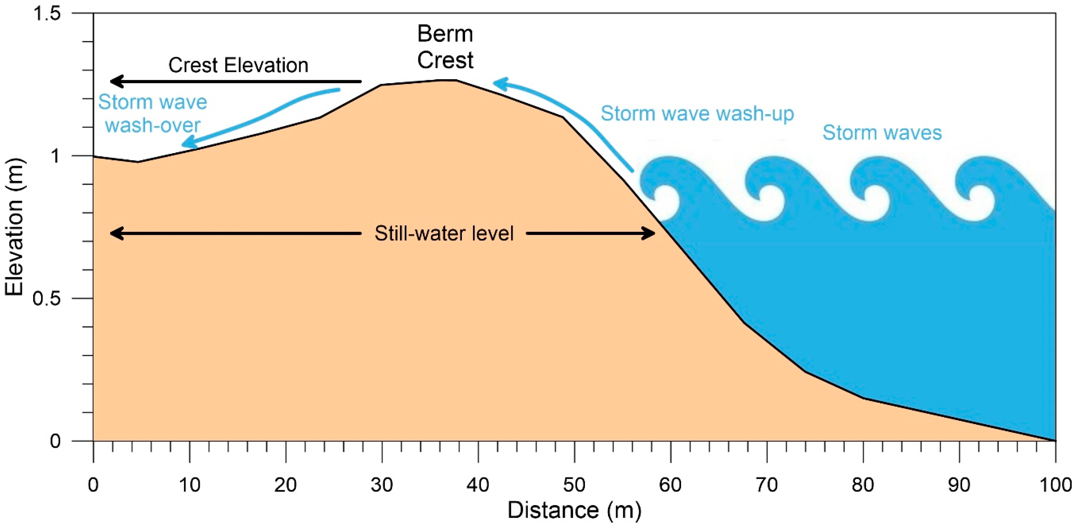
Crest elevations of the shorelines measured along the Tobar transect likely do not correspond directly with the elevation of the water surface at the time when the lake was constructed. These shorelines consist of coarse sand and gravel and were presumably built by large waves driven by storms sweeping across the former lake surface. Observations of the modern Great Salt Lake in Utah have demonstrated that wave run-up can construct beach berms at elevations up to 2 m higher than the still-water surface of the lake [17,18]. Thus, the elevations of the Lake Clover berms mapped and sampled in the field must be adjusted downward to correspond with the former lake surface elevation. Consideration of the measured topographic profile crossing each ridge supported an estimation of the midpoint elevation of the beach face; this was taken as the still-water level on the beach face at the time when each berm was built (Figure 4). These elevations were used in a GIS to determine the dimensions of Lake Clover when each shoreline was produced.
2.4. Laboratory Methods
All 10 of the tubes containing luminescence samples were opened under safe light conditions in the luminescence laboratory at Middlebury College. Sediment from the first and last ~5 cm of each tube was discarded and only the sediment from the tube center was processed for dating. The discarded sediment was dried and passed through a stack of sieves (−1, 0, 1, 2, 3, and 4 ϕ) by shaking on a Rotap sieve shaker for 15 min. The resulting size fractions were weighed and used to calculate the grain size distribution using Gradistat 8.0 [19]. Sediment passing the finest sieve (63 µm, 4 ϕ) was dispersed in distilled water with 3% sodium hexametaphosphate for 1 week and then analyzed in a Horiba LA-950 particle size analyzer with laser scattering. This instrument has an effective range from 10 nm to 3 mm, and a refractive index of 1.54 with an imaginary component of 0.1i was used in calculating the grain size distribution. This analysis provided information about the abundance of silt and clay sized material in these sediments.
For six of the luminescence samples, quartz and feldspar were purified from the central material in each sample tube following standard laboratory procedures, which are explained in more detail in the supplemental material. Mineral grains were then mounted on 9.8-mm aluminum discs for analysis. For quartz, small aliquots (20–50 grains) from each sample were analyzed using the SAR protocol on a Daybreak 2200 reader [20]. Application of typical rejection criteria, including requiring a fast ratio >10, led to acceptance of only ~2% of quartz aliquots. Given the inadequate luminescence behavior of the quartz grains, analysis shifted to applying the ( (pIRIR SAR) protocol to single grains of K-feldspar [21]. pIRIR SAR cycles used a preheat of 250 °C, an initial shine down at 50 °C, a second shine down at 225 °C, and a bleach at 235 °C to end each SAR cycle. Because the luminescence of K-feldspar is considerably brighter than quartz, the rate of accepted discs was much higher (~25%), supporting construction of a more robust geochronological dataset.
The luminescence signal in K-feldspar is prone to anomalous fading and incomplete bleaching; therefore, additional analyses were conducted to constrain the fading rate and measure the unbleachable or ‘residual’ dose. Complete details of all analytical protocols, data reduction steps, and error propagation calculations can be found in the Supplementary Materials.
Once a suitable number of quartz and feldspar aliquots from each sample were accepted, the residual dose was subtracted and a fading correction was applied (feldspar only) [22], and the equivalent dose was divided by the dose rate experienced during burial to estimate an apparent age for the aliquot. Dose rates were determined from the sediment excavated around each tube using high-resolution gamma spectrometry at Dartmouth College to measure the activity of 40K as well as certain isotopes in the 238U and 232Th decay chains. These activities were then converted to in situ dose rates using standard conversion parameters [23] and the DRAC calculator v. 1.2 [24]. Because the dose rate experienced by feldspar is partially derived from internal 40K, the potassium content of the K-feldspar was determined by EDS analysis of polished grains using a Vega Tescan3 SEM at Middlebury College. The mean K content of 18 individual grains (10.7 ± 1.4 wt. %) was then applied to all samples.
Because the multiple aliquots analyzed from each sample generate a distribution of apparent ages, an age model is necessary to estimate a single burial age for the sediment. To this end, the distribution of ages and uncertainties for each sample were passed into the R-package “Luminescence” for plotting and age estimation [25]. Ages were calculated using the central age model (CAM) for all distributions [26]. For feldspar, the CAM is justified by 0% over-dispersion for all samples. For quartz, this approach is justified by the relatively small number of accepted aliquots, which did not lend confidence in the alternative minimum age model (MAM).
3. Results
3.1. Surveying
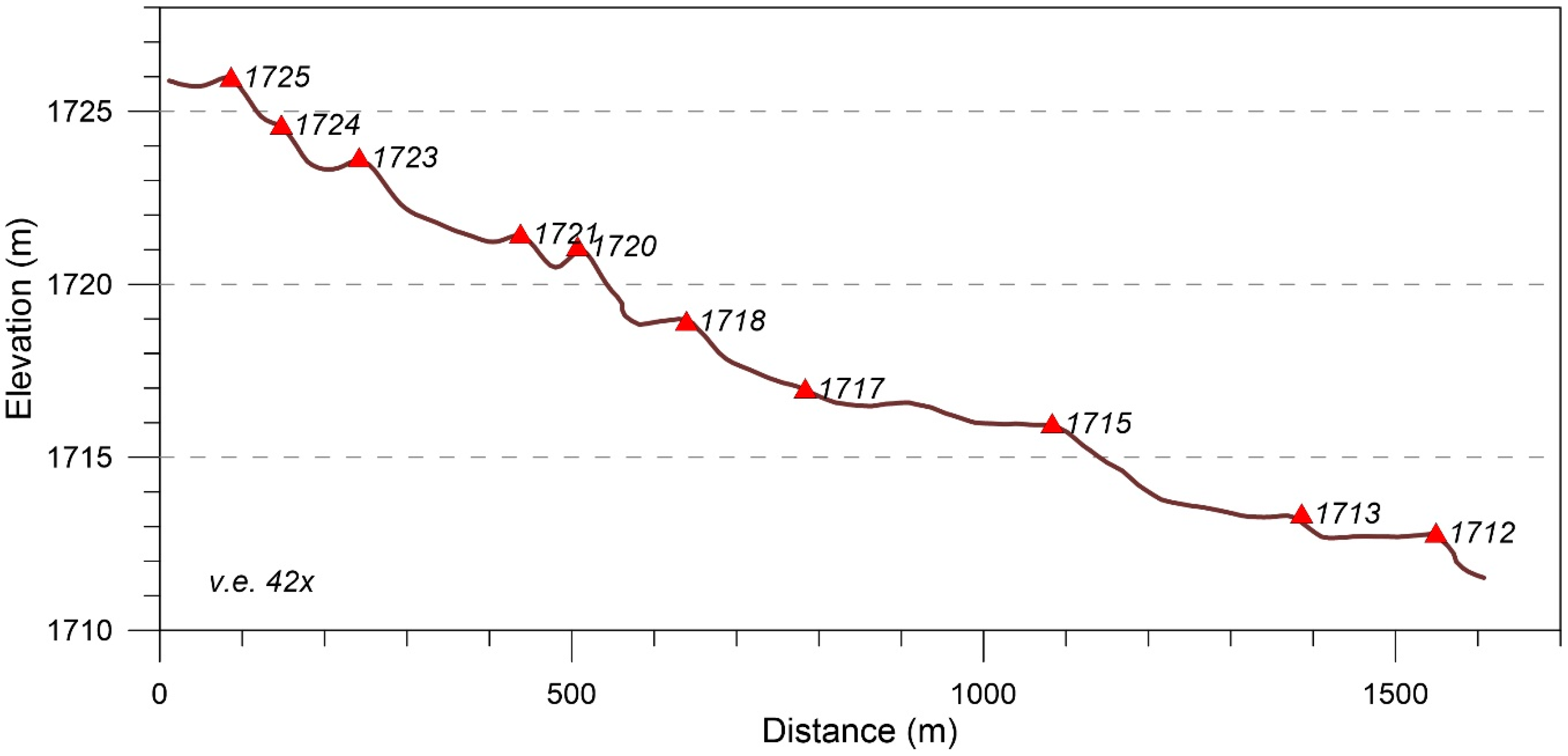
Aerial photography and field reconnaissance confirm the presence of 10 shorelines built by Lake Clover at the Tobar transect. Topographic surveying with the total station, combined with the vertical adjustment detailed in Figure 4, indicates that shorelines were built when Lake Clover stood at elevations of 1725, 1724, 1723, 1721, 1720, 1718, 1717, 1715, 1713, and 1712 m (Figure 5).
The highstand beach at 1725 m is found in close proximity to two others that collectively form a triplex at the highest elevations reached by the lake. Below this group of ridges, two more shorelines were built when Lake Clover stood at 1721 and 1720 m. The higher of these ridges is discontinuous and appears to merge with the more prominent lower ridge to the east (Figure 2). The next ridge down, built by a lake at 1718 m, represents a topographic departure from the higher ridges, which follow on contour around the alluvial fan, and the lower ridges, which wrap out to a former island in Lake Clover (Figure 1). This shoreline is the highest to extend out to the island as a narrow tombolo. A ridge at 1717 m is discontinuous and topographically subtle. Of the lowest three ridges built by Lake Clover at 1715, 1713, and 1712 m, the intermediate ridge is also discontinuous but the other two are easy to follow across the study area (Figure 1).
3.2. Spatial Analysis
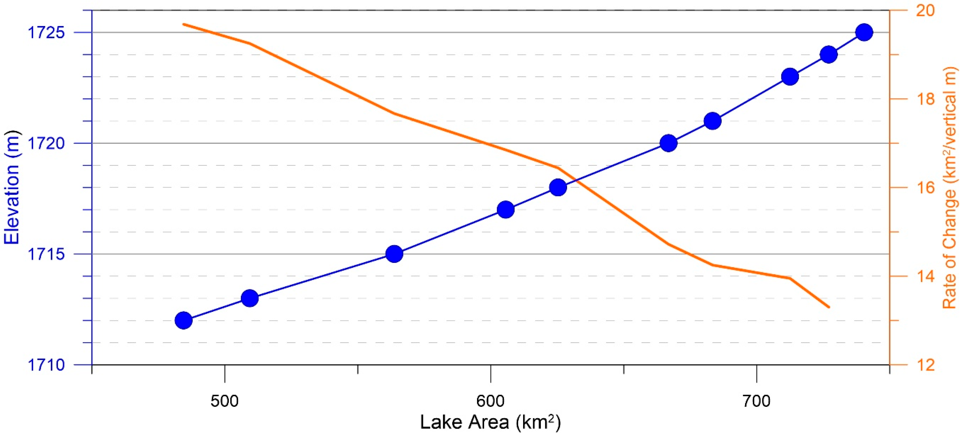
Spatial analysis in a GIS using the elevations of these shorelines permit estimation of the dimensions of Lake Clover when each of the 10 berms was constructed. This quantification reveals that Lake Clover covered 740 km2 at its maximum extent, and ~485 km2 when the lowest shoreline was constructed (Figure 6). At this time, the lake covered 65% of its maximum area. The hypsometry of the lake varies at an increasing rate at lower elevations (Figure 6). The area change per elevation change from one shoreline to the next is ~14 km2/vertical m for the highest shorelines, to ~19 km2/vertical m for the lower shorelines (Table 1).
3.3. Sedimentology and Stratigraphy
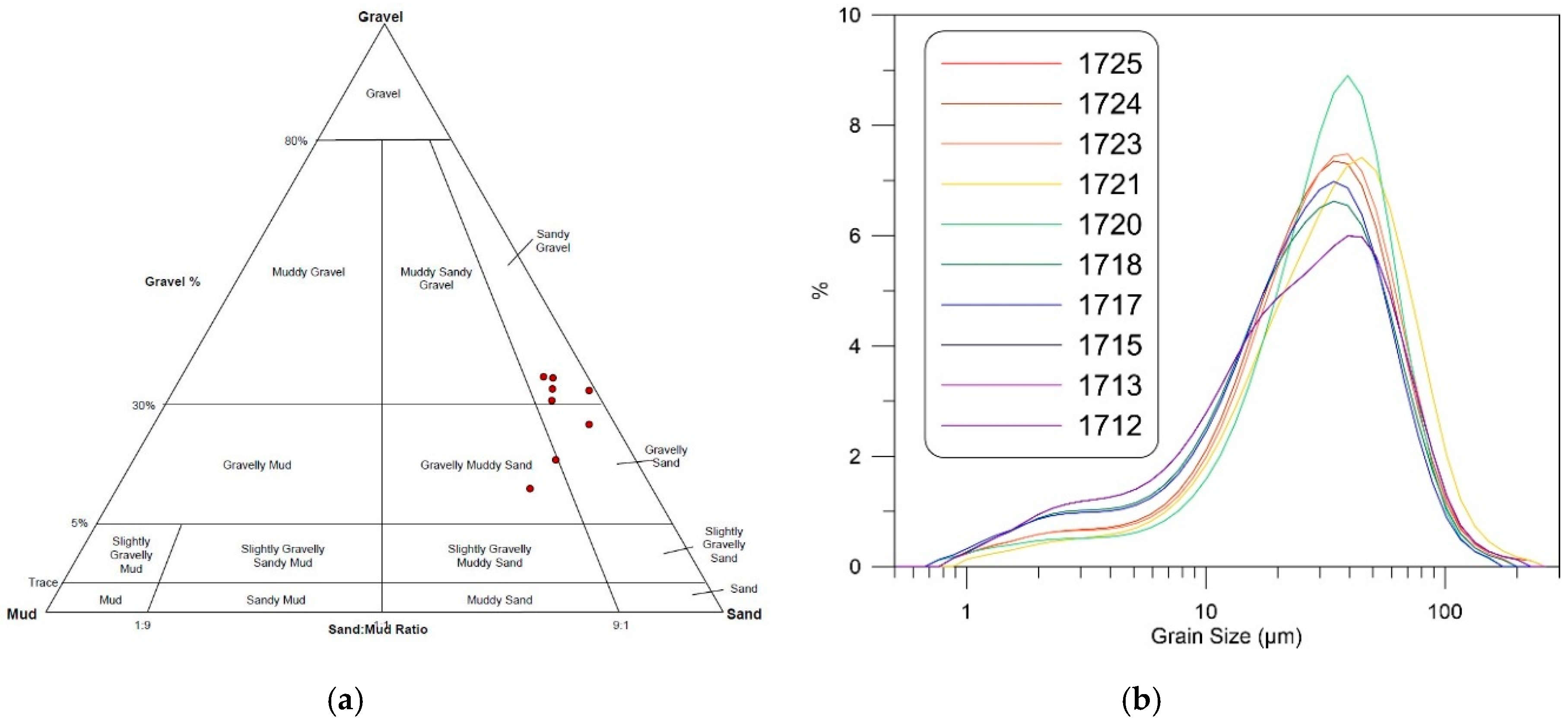
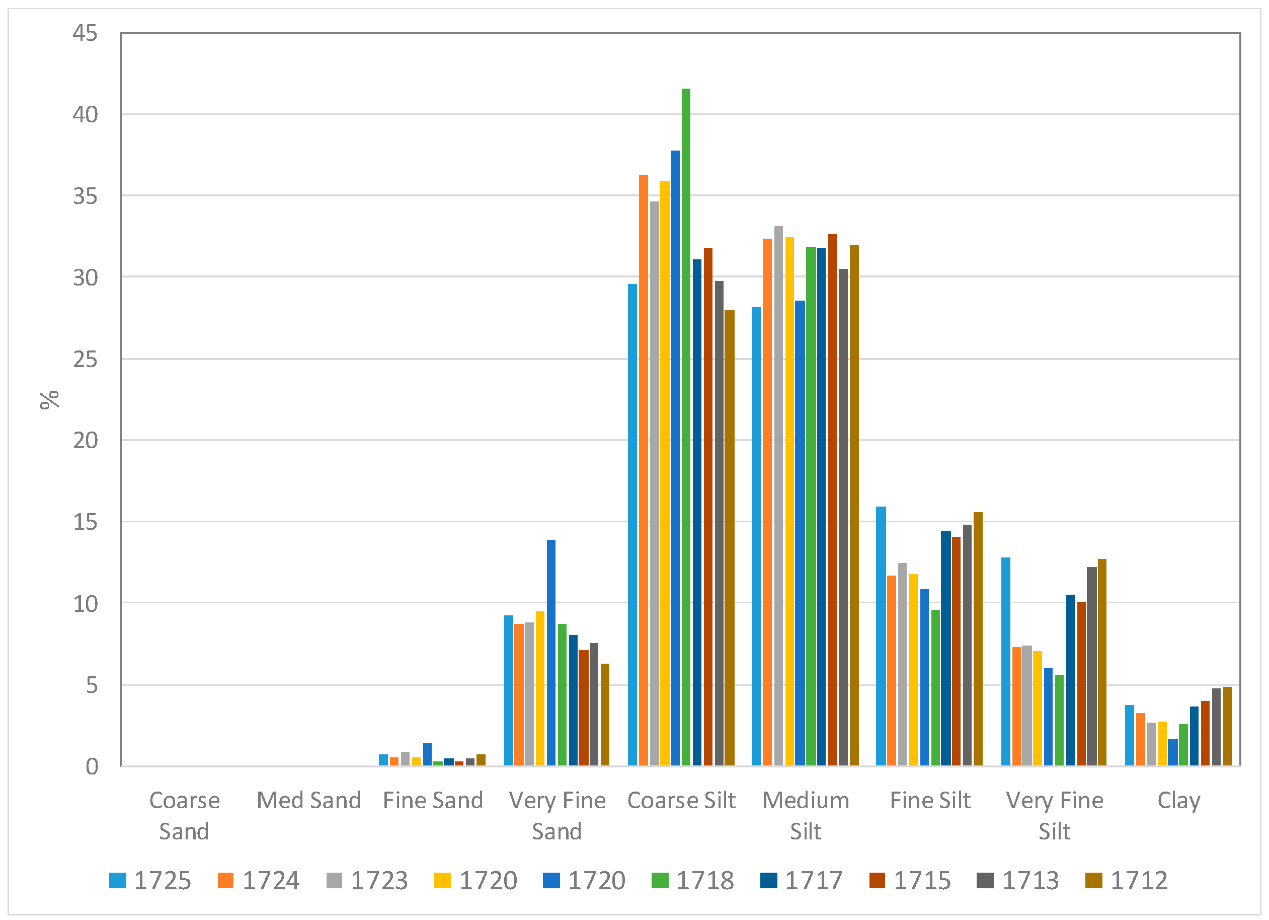
On a ternary diagram of mud, sand, and gravel, nearly all samples of sediments comprising the Lake Clover shorelines classify as gravelly sand and sandy gravel. One sample (1725) is slightly finer and classifies as a gravelly muddy sand (Figure 7). The fine fraction (<63 um) analyzed with laser scattering has a mean of 27 to 37 µm, with an overall mean of 31 µm (Figure 7). Coarse silt (63–30 µm) and medium silt (30–14 µm) are the most common grain size classes in the fine fraction, with each generally comprising >30% of each sample. Clay (<2 µm) makes up <5% of the fine fraction for all samples (Figure 8).
Stratigraphically, the unconsolidated sediments forming these ridges are arranged in layers from 5 to 20 cm thick (Figure 9). Lenses of gravel poor/sand dominant sediment are locally present. At the scale of the hand excavations, it was not possible to determine whether the layers deviate from horizontal. The coarser gravel layers are faintly imbricated. A layer of relatively gravel-poor silt from 15 to 20 cm thick interpreted as loess caps each shoreline. Beneath this silt in all shorelines is a layer of gravelly sand 25 to 55 cm thick. In some excavations, this gravelly sand locally transitions to a finer silty gravel at depth. These basic types of sediment are present in all of the described exposures (Figure 10). However, in the lowest three shorelines, the loess layer is less distinct and gravelly sand makes up a greater proportion of the stratigraphy (Figure 10). Some excavations encountered a matrix-poor, openwork layer of fine gravel at depth that readily caved into the pit, making deeper excavation difficult. Other excavations reached a dense silt layer at a depth of 80–120 cm that similarly halted further penetration. The pits at 1721, 1720, 1713, and 1712 reached a nearly pure sand layer >65 cm below the surface. The excavations in the 1725, 1723, and 1715 shorelines reached a carbonate cemented layer. This horizon forms the floor of alluvial gully along the railroad tracks near the exposure through the 1715 ridge.
Soil profiles exposed in all of the excavations are minimally developed Aridisols. Each profile is capped by an Av horizon, roughly corresponding to the loess layer, from 20 to 30 cm thick with a Munsell color of 10YR 6/3 (pale brown). 2Bw horizons developed in the gravelly sand beneath the Av range from 20 to 50 cm thick with slightly lighter 10YR 6/4 colors (light yellowish brown). 2C horizons encountered in some pits had colors of 7.5YR 6/4 (light brown) to 7.5YR 5/6 (strong brown). Two pits reached a 3C horizon, with very pale brown colors (10YR 8/2, 1717 m), (10YR 7/4, 1715 m).
3.4. Luminescence Dating
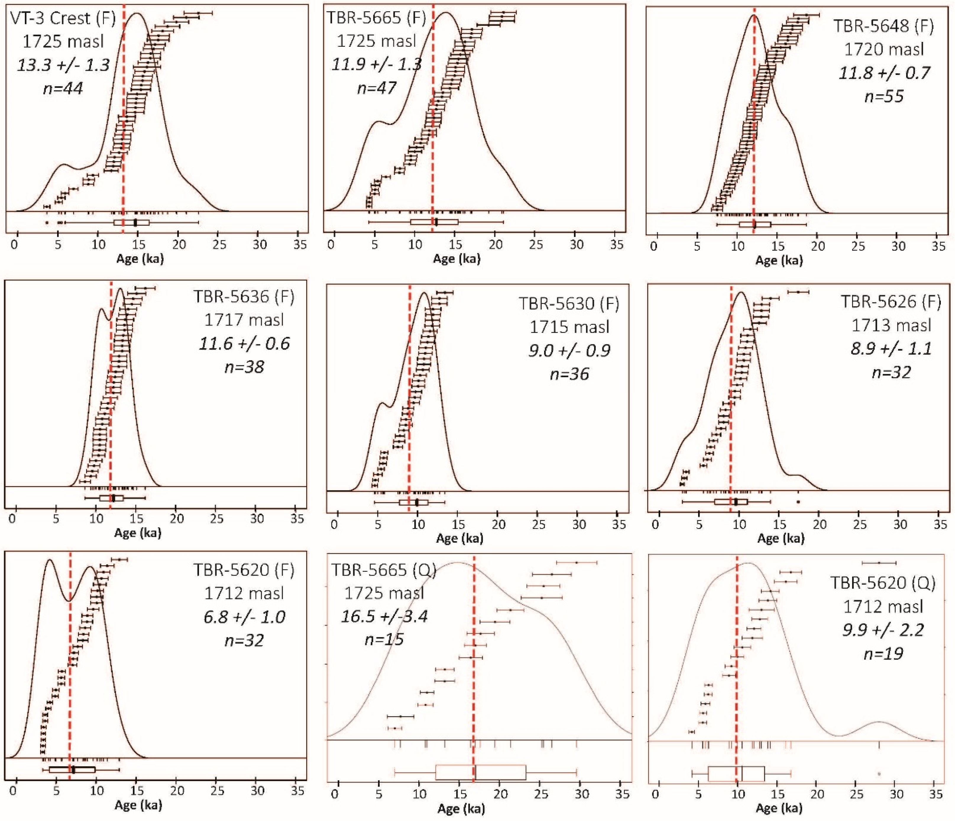
Six of the shoreline berms sampled at the Tobar transect were dated using pIRIR SAR analysis of feldspar: 1725, 1720, 1717, 1715, 1713, and 1712 m. Figure 11 and Table 2 illustrate that feldspar ages range from 15.9 ± 1.9 ka on the highstand shoreline to 9.5 ± 1.4 ka on the lowest ridge (all age ranges reported at ±2-σ). The highest and lowest ridges were also dated using quartz SAR to cross-check the feldspar results. Sample TBR-5665 from the highstand ridge yielded a quartz SAR age of 16.5 ± 3.4 ka matching the feldspar pIRIR SAR age. Similarly, sample TBR-5620 from the lowstand ridge yielded a quartz SAR age of 9.9 ± 2.2 ka overlapping the feldspar pIRIR SAR age (Figure 11, Table 2).
It is worth noting that most of the K-feldspar samples contain a young population of single grain ages, which in some cases suggests a bimodal population of grains with a younger population near 5 ka. Although it is tempting to assign younger depositional ages to these samples we argue that the older ages inferred from the CAM are more appropriate due to: (1) the large uncertainties introduced by the residual dose correction (see Supplementary Materials), and (2) the relatively shallow sampling depth above the soil carbonate horizon, which leaves open the possibility of sample contamination by bioturbation.
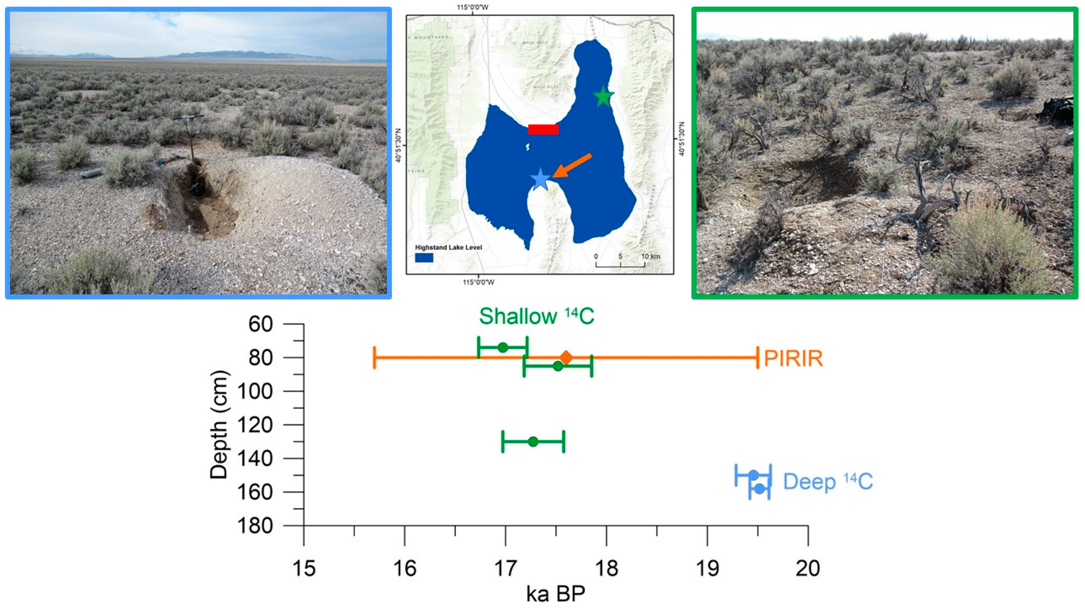
Further confidence in the luminescence results is provided by a sample collected from the highstand shoreline at Ventosa in the south-central part of the area covered by Lake Clover (“V” in Figure 1). This sample, from a depth of 80 cm below the ridge crest, yielded a feldspar pIRIR SAR age of 17.6 ± 1.9 ka. This result overlaps with the age for the highstand shoreline at Tobar (K-feldspar 15.9 ± 1.9 ka, quartz 16.5 ± 3.4 ka) and exhibits strong consistency with two 14C ages (~17 to 17.5 cal ka BP) from same depth (74–85 cm) in the highstand shoreline at a site in the northeast Independence Valley (“I” in Figure 1). Radiocarbon dating of gastropod shells from ~150 cm at Ventosa yielded older ages of ~19 cal ka BP, which nonetheless fall within the distal ranges of the error bars on the pIRIR SAR result (Figure 12). It is possible that Lake Clover reached its highstand elevation twice, first ca. 19 ka, and again ca. 17 ka [14]. Either way, the correspondence between the pIRIR SAR age and the available 14C control is strong confirmation that the luminescence ages are not subject to a systematic bias.
4. Discussion
4.1. Shoreline Chronology
The highstand shoreline of Lake Clover at the Tobar transect was constructed ca. 16 ka, matching the luminescence and 14C ages for this shoreline from elsewhere in the Clover and Independence Valleys. The prominent shoreline at 1720 m was constructed ca. 15.2 ± 1.5 ka, and the shoreline at 1717 m was built at 14.9 ± 1.7 ka. Thus, the upper seven Lake Clover shorelines were built over roughly 1000 years between ~16 and 15 ka. During this time, the surface elevation of Lake Clover fell ~8 m, and the area of the lake decreased 18% to 606 km2 (Table 1).
The next two shorelines, constructed by a lake at 1715 and 1713 m, were both built notably later, ca. 11.5–12.0 ka. At this time, the lake covered 69 to 76% of its original highstand area. From the available evidence, it is not possible to determine where Lake Clover stood between the formation of the first and second groups of shorelines. It is possible that the lake fell to a much lower elevation, or even disappeared entirely, before transgressing to build its final shoreline. However, there is no evidence in the topographic profile or the geochronology to support or refute this possibility.
The final shoreline of Lake Clover was constructed ca. 9.5 ± 1.4 ka when the lake covered 65% of its highstand area (Table 1) to a maximum depth of 9 m. No shorelines have been identified in the basin at elevations <1712 m. It is possible that all shorelines at lower elevations have been eliminated by erosion or buried by sediment. However, given the extent of the basin, it seems unlikely that every trace of lower shorelines has been removed. More plausible is that lower shorelines were never constructed, either because the final regression of the lake was too rapid or because the increasingly shallow water depth prohibited the formation of larger storm waves necessary to build storm berms.
The properties of the sediments comprising the Lake Clover beach ridges, as well as their internal stratigraphy, are consistent with this interpretation of the luminescence results. The sandy gravel alternating with open-work gravel and layers of pure sand encountered in excavations into these ridges are typical of wave-washed, high-energy coastal environments. Similar sediments have been reported from other studies of pluvial lake beaches in the Great Basin [5,13,27]. None of the ridges contain stratigraphic evidence, such as finer-grained deepwater sediments, consistent with submergence by later high water, which would indicate a complicated history of lake level rise and fall. All of the ridges are capped by a layer of loess that postdates ridge formation (Figure 10). This loess exhibits a reduced contrast with the underlying sediment in the lowest three shorelines. This difference is consistent with the apparently younger age of these features. Together, these results are consistent with stepwise regression of the lake after construction of the highstand shoreline.
Figure 13 plots the calculated ages for Lake Clover shorelines against the fraction of the highstand lake area covered when each shoreline was constructed. It is clear that the lake reached its highstand during Heinrich Stadial 1 [28,29] (Greenland Stadial GS-2 in the INTIMATE Event Chronology [30]), followed by a regression into the Bølling/Allerød (GI-1). Two of the lower shorelines were built during or at the end of the Younger Dryas episode (GS-1), and the lowest shoreline was constructed in the early Holocene.
4.2. Comparison with Other Records and Paleoclimate Implications
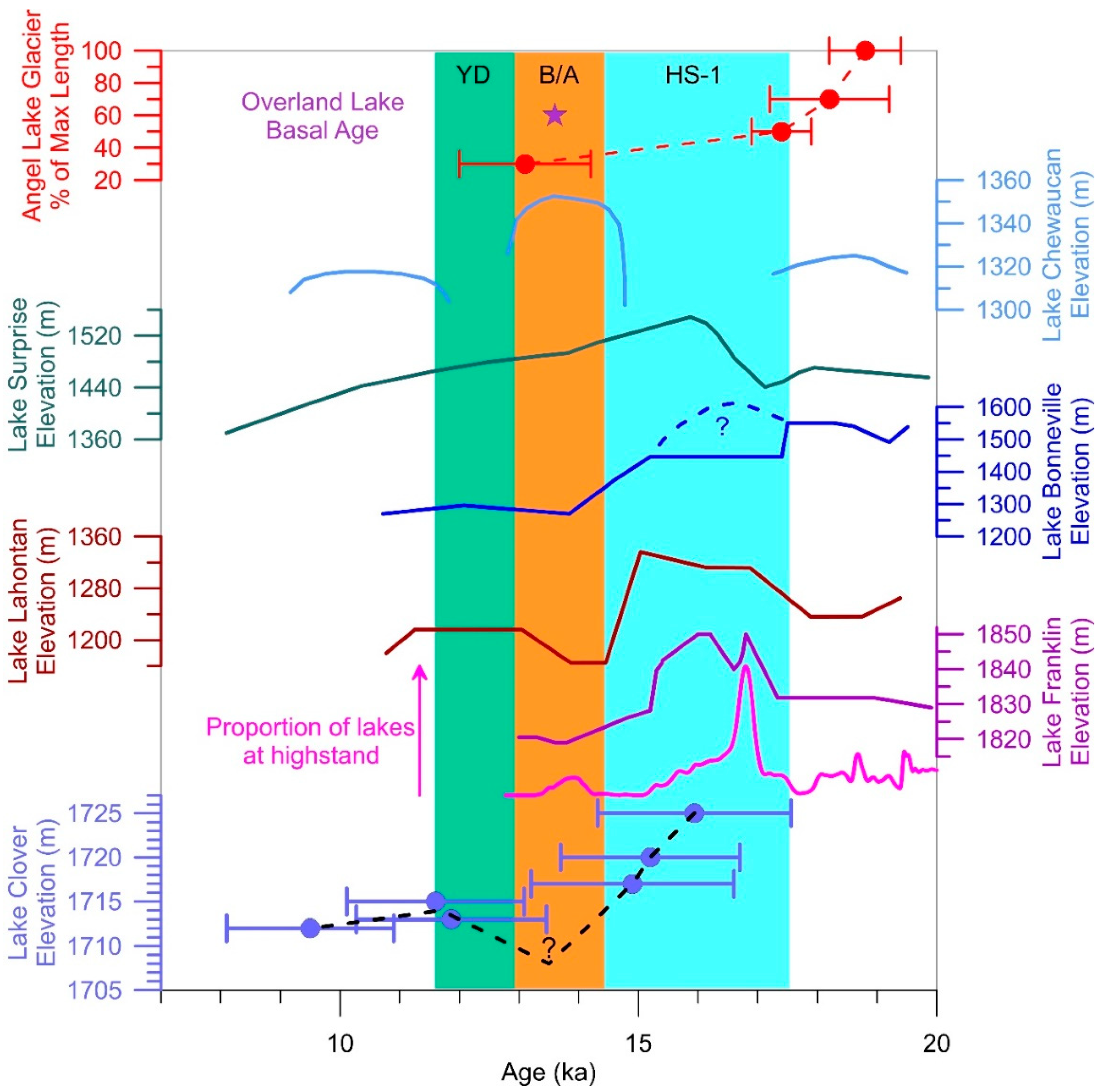
This new chronology for the highstand and subsequent regression of Lake Clover provides a useful point of comparison with existing hydroclimate records from the last glacial-interglacial transition in the northern Great Basin. Most striking is the correspondence of the Lake Clover highstand with other radiocarbon-based lake chronologies (Figure 14); construction of the highstand beach ridge of Lake Clover ca. 16 ka is synchronous within error with the dated highstands of Lake Surprise [31] in northern California, Lake Lahontan [32] in western Nevada, and Lake Franklin [13] in the valley adjacent to Lake Clover during Heinrich Stadial 1. This age also falls within the overflowing interval of Lake Bonneville [6], when the ultimate peak of effective moisture is unknown. Looking more broadly, the Lake Clover highstand is consistent with a compilation of lake highstands from across southwestern North America [14], which clearly demonstrates a clustering of lake highstands between 16 and 17 ka.
The regression of Lake Clover late in Heinrich Stadial 1 also matches falling water levels in the other well-dated lakes and a major decrease in the number of lakes at their highstand levels in the regional compilation (Figure 14). The elevation of Lake Clover during the Bølling/Allerød warm interval, or even if the lake existed at all, is unknown. However, evidence for low water levels has also been reported from Lakes Bonneville [6], Franklin [13], and Lahontan [32] at this time (Figure 14).
Construction of shorelines by Lake Clover at ca. 1715 m during the Younger Dryas coincides with minor transgressions in other well-dated lake records. For instance, Lake Franklin rose slightly to construct a shoreline after ~13 ka BP [13]. Lake Lahontan rose over 50 m between 13.1 and 11.7 ka BP, as constrained by a prominent wave-cut terrace in Pyramid Lake [32]. Lake Bonneville transgressed during the Gilbert Episode, reaching an elevation of 1296 m ca. 11.6 ka BP [34].
Together, this pattern of lake highstands during Heinrich Stadial 1, regression during the Bølling/Allerød, and minor transgression during the Younger Dryas fits with the theory that stadial (colder) conditions in the North Atlantic enhanced effective moisture in the Great Basin, whereas interstadial (warmer) conditions reduce effective moisture. This teleconnection may involve changes in the position of the intertropical convergence zone and the polar jet stream [11,12], or is perhaps related more to interactions between the Laurentide Ice Sheet and high pressure systems in the North Pacific [10]. Either way, the new hydrograph for Lake Clover reported here strongly supports the idea that hydroclimate in the Great Basin was connected with events in the North Atlantic during the last glacial-interglacial transition.
The hydrograph for Lake Clover also helps reinforce the recently proposed theory that lakes at the northernmost extent of the Great Basin in Oregon reached their highstands out of phase with those at the latitude of northern Nevada. The evidence in support of this idea comes from Lake Chewaucan in south-central Oregon (42.8° N), which was apparently low during Heinrich Stadial I, reached a highstand during the Bølling/Allerød, and regressed again during the Younger Dryas—a pattern in complete opposition to Lakes Franklin (40.1° N), Lahontan (39.8° N), and Surprise (41.5° N) [9]. Lake Clover, at 40.8° N, fits perfectly with the pattern of the other lakes in the ~40–41° N latitude band, with a highstand and subsequent regression that clearly predate Lake Chewaucan (Figure 13). Drying of lakes in northern Nevada, at the same time that lakes farther north transgressed in response to increased effective moisture, is consistent with a northern migration of the Pacific storm track during the Bølling/Allerød [9].
Other local, non-pluvial paleoclimate records provide additional context for considering the Lake Clover hydrograph. As noted in Figure 1, Lake Clover was located immediately east of the East Humboldt Mountains that hosted numerous alpine glaciers during the last glaciation. A well-preserved set of terminal and lateral moraines down-valley from Angel Lake (Figure 1c) was designated as the type locality for the Last Glacial Maximum in the Great Basin [15]. Surface-exposure dating of these moraines using cosmogenic 10Be reveals that the Angel Lake Glacier began to retreat from its terminal moraine ca. 18.8 ± 0.6 ka (recalculated from [33]). Additional recessional moraines were built ca. 18.2 ± 1.0 and 17.4 ± 0.5 ka as the glacier retreated to ~50% of its maximum length. A final recessional moraine impounding Angel Lake was constructed ca. 13.1 ± 1.1 ka, when the glacier length was just 30% of its maximum extent. A calibrated basal 14C date of 13.5 ka from Overland Lake in the East Humboldt Mountains also indicates that the glacier in this valley had retreated to <25% its maximum length by this time [16]. Overall, this pattern is consistent with the idea that the local glacier maximum was driven by cold, relative dry conditions that favored ice advance but not tremendous increases in effective moisture. Later pluvial highstands occurred under relatively cool, but wetter conditions [13].
Perhaps the most unexpected aspect of the Lake Clover hydrograph is the evidence that the lake persisted into the early Holocene. As noted above, the lowest shoreline of the lake (at 1712 m) was dated by both quartz SAR and K-feldspar pIRIR SAR techniques to ca. 10 ka. At this time, the lake was smaller than its extent during the Younger Dryas, but still covered ~65% of its highstand area (Table 1). This result indicates that effective moisture in the Lake Clover watershed was still considerably greater than modern at this time. One possible mechanism for maintaining Lake Clover into the early Holocene is an enhanced North American monsoon driven by the summer insolation maximum [35,36]. Paleoclimate records from elsewhere in the southwestern U.S. indicate that the monsoon was well established by 9 ka [37]. On the other hand, water levels were apparently low in high-elevation lakes in the Ruby Mountains ~50 km southwest of Lake Clover at this time [16], and paleobotanical data from Blue Lake ~100 km east of Lake Clover in the Bonneville Basin indicate arid conditions between 11 and 9.5 ka [38]. It is currently unclear how to resolve the apparent discrepancy between these paleoclimate records. However, confirming the presence a relatively large lake driven by increased effective moisture in the Clover and Independence Valleys during the early Holocene could have important implications for paleoclimate reconstructions and archeology in this part of the Great Basin.
5. Conclusions
Pluvial Lake Clover occupied parts of the Clover and Independence Valleys of northeastern Nevada during the last glacial-interglacial transition. Luminescence dating, using the SAR protocol for quartz and the pIRIR SAR protocol for K-feldspar, indicates that the lake stood at its highstand elevation of 1725 m ca. 16 ka. The lake regressed late in Heinrich Stadial 1, synchronous with falling water levels of other well-dated lakes from the northern Great Basin. The configuration (or existence) of the lake during the Bølling/Allerød is unclear; however, the lake did build additional shorelines during the Younger Dryas interval. A final shoreline was constructed ca. 10 ka in the early Holocene, when the lake covered ~65% of its maximum area. Overall, the hydrograph of Lake Clover exhibits a striking correspondence with other lakes in the ~40–41° N latitude band and provides support for the theory that the Pacific storm track was steered over this region during Heinrich Stadial 1 before retreating northward during the Bølling/Allerød. Persistence of the lake into the early Holocene should be investigated further and could have important implications for paleoclimate reconstructions and archeology in this region.
Supplementary Materials
Details about the luminescence dating methods are provided in the supplemental methods file. The following are available online at https://0-www-mdpi-com.brum.beds.ac.uk/2571-550X/3/2/11/s1.
Author Contributions
Conceptualization, J.S.M.; methodology, J.S.M., C.K.W., and W.H.A.; software, W.H.A.; validation, J.S.M. and W.H.A.; formal analysis, J.S.M., C.K.W., W.H.A., and J.D.L.; investigation, J.S.M. and C.K.W.; resources, J.S.M. and W.H.A.; data curation, J.S.M. and W.H.A.; writing—original draft preparation, J.S.M.; writing—review and editing, J.S.M. and W.H.A.; visualization, J.S.M. and W.H.A.; supervision, J.S.M. and W.H.A.; project administration, J.S.M.; funding acquisition, J.S.M. and W.H.A. All authors have read and agree to the published version of the manuscript.
Funding
This research was funded by the U.S. National Science Foundation, grant number P2C2-17-02975 to J.S.M. and W.H.A.
Acknowledgments
C.K.W. received support from the Undergraduate Research Office at Middlebury College. B.K.B., J.K.H., and K.R. provided significant assistance in the field.
Conflicts of Interest
The authors declare no conflict of interest.
References
- Poage, M.; Chamberlain, C. Stable isotopic evidence for a pre-Middle Miocene rain shadow in the western Basin and Range: Implications for the paleotopography of the Sierra Nevada. Tectonics 2002, 21, 16-1–16-10. [Google Scholar] [CrossRef]
- Mifflin, M.D.; Wheat, M.M. Pluvial Lakes and Estimated Pluvial Climates of Nevada; Nevada Bureau of Mines and Geology: Reno, NV, USA, 1979; Volume 94. [Google Scholar]
- Gilbert, G.K. Lake Bonneville; U. S. Geological Survey: Reston, VA, USA, 1890; p. 438.
- Russell, I.C. Geological History of Lake Lahontan, a Quaternary Lake of Northwestern Nevada; U. S. Geological Survey: Reston, VA, USA, 1885; p. 288.
- Adams, K.D.; Wesnousky, S.G. Shoreline processes and the age of the Lake Lahontan highstand in the Jessup Embayment, Nevada. Geol. Soc. Am. Bull. 1998, 110, 1318–1332. [Google Scholar] [CrossRef]
- Benson, L.V.; Lund, S.P.; Smoot, J.P.; Rhode, D.E.; Spencer, R.J.; Verosub, K.L.; Louderback, L.A.; Johnson, C.A.; Rye, R.O.; Negrini, R.M. The rise and fall of Lake Bonneville between 45 and 10.5 ka. Quat. Int. 2011, 235, 57–69. [Google Scholar] [CrossRef] [Green Version]
- Reheis, M.C. Extent of Pleistocene Lakes in the Western Great Basin; U. S. Geological Survey: Reston, VA, USA, 1999.
- Menking, K.M.; Anderson, R.Y.; Shafike, N.G.; Syed, K.H.; Allen, B.D. Wetter or colder during the Last Glacial Maximum? Revisiting the pluvial lake question in southwestern North America. Quatern.Res. 2004, 62, 280–288. [Google Scholar] [CrossRef]
- Hudson, A.M.; Hatchett, B.J.; Quade, J.; Boyle, D.P.; Bassett, S.D.; Ali, G.; Marie, G. North-south dipole in winter hydroclimate in the western United States during the last deglaciation. Sci. Rep. 2019, 9, 4826. [Google Scholar] [CrossRef] [Green Version]
- Oster, J.L.; Ibarra, D.E.; Winnick, M.J.; Maher, K. Steering of westerly storms over western North America at the last glacial maximum. Nat. Geosci. 2015, 8, 201–205. [Google Scholar] [CrossRef]
- Asmerom, Y.; Polyak, V.J.; Burns, S.J. Variable winter moisture in the southwestern United States linked to rapid glacial climate shifts. Nat. Geosci. 2010, 3, 114–117. [Google Scholar] [CrossRef]
- Wagner, J.D.M.; Cole, J.E.; Beck, J.W.; Patchett, P.J.; Henderson, G.M.; Barnett, H.R. Moisture variability in the southwestern United States linked to abrupt glacial climate change. Nat. Geosci. 2010, 3, 110–113. [Google Scholar] [CrossRef]
- Munroe, J.S.; Laabs, B.J. Latest Pleistocene history of pluvial Lake Franklin, northeastern Nevada, USA. Geol. Soc. Am. Bull. 2013, 125, 322–342. [Google Scholar] [CrossRef] [Green Version]
- Munroe, J.S.; Laabs, B.J. Temporal correspondence between pluvial lake highstands in the southwestern US and Heinrich Event 1. J. Quat. Sci. 2013, 28, 49–58. [Google Scholar] [CrossRef]
- Sharp, R.P. Pleistocene glaciation in the Ruby-East Humboldt Range, northeastern Nevada with abstract in German by Kurt E. Lowenstein. J. Geomorphol. 1938, 1, 296–323. [Google Scholar]
- Munroe, J.S.; Bigl, M.F.; Silverman, A.E.; Laabs, B.J. Records of late Quaternary environmental change from high-elevation lakes in the Ruby Mountains and East Humboldt Range, Nevada. In From Saline to Freshwater: The Diversity of Western Lakes in Space and Time; Geological Society of America Special Paper 536; Starratt, S.W., Rosen, M.R., Eds.; Geological Society of America: Boulder, CO, USA, 2019. [Google Scholar]
- Atwood, G. Geomorphology applied to flooding problems of closed-basin lakes … specifically Great Salt Lake, Utah. In Geomorphology and Natural Hazards; Morisawa, M., Ed.; Elsevier: Amsterdam, The Netherlands, 1994; pp. 197–219. ISBN 978-0-444-82012-9. [Google Scholar]
- Atwood, G.; Wambeam, T.J.; Anderson, N.J. Chapter 1—The Present as a Key to the Past: Paleoshoreline Correlation Insights from Great Salt Lake. In Developments in Earth Surface Processes; Oviatt, C.G., Shroder, J.F., Eds.; Elsevier: Amsterdam, Netherlands, 2016; Volume 20, pp. 1–27. [Google Scholar]
- Blott, S.J.; Pye, K. GRADISTAT: A grain size distribution and statistics package for the analysis of unconsolidated sediments. Earth Surf. Process. Landf. 2001, 26, 1237–1248. [Google Scholar] [CrossRef]
- Murray, A.S.; Wintle, A.G. Luminescence dating of quartz using an improved single-aliquot regenerative-dose protocol. Radiat. Meas. 2000, 32, 57–73. [Google Scholar] [CrossRef]
- Buylaert, J.-P.; Murray, A.S.; Thomsen, K.J.; Jain, M. Testing the potential of an elevated temperature IRSL signal from K-feldspar. Radiat. Meas. 2009, 44, 560–565. [Google Scholar] [CrossRef]
- Huntley, D.J.; Lamothe, M. Ubiquity of anomalous fading in K-feldspars and the measurement and correction for it in optical dating. Can. J. Earth Sci. 2001, 38, 1093–1106. [Google Scholar] [CrossRef]
- Adamiec, G.; Aitken, M.J. Dose-rate conversion factors: Update. Anc. Tl 1998, 16, 37–50. [Google Scholar]
- Durcan, J.A.; King, G.E.; Duller, G.A. DRAC: Dose Rate and Age Calculator for trapped charge dating. Quat. Geochronol. 2015, 28, 54–61. [Google Scholar] [CrossRef] [Green Version]
- Kreutzer, S.; Schmidt, C.; Fuchs, M.C.; Dietze, M.; Fischer, M.; Fuchs, M. Introducing an R package for luminescence dating analysis. Anc. Tl 2012, 30, 1–8. [Google Scholar]
- Galbraith, R.F.; Roberts, R.G.; Laslett, G.; Yoshida, H.; Olley, J.M. Optical dating of single and multiple grains of quartz from Jinmium Rock Shelter, northern Australia: Part I, experimental design and statistical models*. Archaeometry 1999, 41, 339–364. [Google Scholar] [CrossRef]
- Smith, K.M.; McBride, J.H.; Nelson, S.T.; Keach, R.W.; Hudson, S.M.; Tingey, D.G.; Rey, K.A.; Carling, G.T. An integrated high-resolution geophysical and geologic visualization of a Lake Bonneville shoreline deposit (Utah, USA). Interpretation 2019, 7, T265–T282. [Google Scholar] [CrossRef]
- Bond, G.C.; Heinrich, H.; Broecker, W.S.; Labeyrie, L.D.; McManus, J.; Andrews, J.; Huon, S.; Jantschik, R.; Clasen, S.; Simet, C.; et al. Evidence for massive discharges of icebergs into the North Atlantic ocean during the last glacial period. Nature 1992, 360, 245–249. [Google Scholar] [CrossRef]
- Hemming, S.R. Heinrich events; massive late Pleistocene detritus layers of the North Atlantic and their global climate imprint. Rev. Geophys. 2004, 42, RG1005.1–RG1005.43. [Google Scholar] [CrossRef] [Green Version]
- Rasmussen, S.O.; Bigler, M.; Blockley, S.P.; Blunier, T.; Buchardt, S.L.; Clausen, H.B.; Cvijanovic, I.; Dahl-Jensen, D.; Johnsen, S.J.; Fischer, H. A stratigraphic framework for abrupt climatic changes during the Last Glacial period based on three synchronized Greenland ice-core records: Refining and extending the INTIMATE event stratigraphy. Quat. Sci. Rev. 2014, 106, 14–28. [Google Scholar] [CrossRef] [Green Version]
- Egger, A.E.; Ibarra, D.E.; Widden, R.; Langridge, R.M.; Marion, M.; Hall, J. Influence of pluvial lake cycles on earthquake recurrence in the northwestern Basin and Range, USA. Geol. Soc. Am. Spec. Pap. 2018, 536, 1–28. [Google Scholar]
- Benson, L.; Smoot, J.; Lund, S.; Mensing, S.; Foit Jr, F.; Rye, R. Insights from a synthesis of old and new climate-proxy data from the Pyramid and Winnemucca lake basins for the period 48 to 11.5 cal ka. Quat. Int. 2013, 310, 62–82. [Google Scholar] [CrossRef] [Green Version]
- Munroe, J.S.; Laabs, B.J.C.; Oviatt, C.G.; Jewell, P.W. New Investigations of Pleistocene Pluvial and Glacial Records from the Northeastern Great Basin. In Sixth International Limnogeology Congress—Field Trip Guidebook, Reno, Nevada, June 15–19, 2015; Rosen, M.R., Ed.; USGS: Reston, VA, USA, 2015; pp. 1–60. [Google Scholar]
- Oviatt, C.G. The Gilbert Episode in the Great Salt Lake Basin, Utah; Utah Geological Survey: Salt Lake City, UT, USA, 2014. [Google Scholar]
- Diffenbaugh, N.S.; Ashfaq, M.; Shuman, B.; Williams, J.W.; Bartlein, P.J. Summer aridity in the United States: Response to mid-Holocene changes in insolation and sea surface temperature. Geophys. Res. Lett. 2006, 33, L22712. [Google Scholar] [CrossRef] [Green Version]
- Zhao, Y.; Harrison, S.P. Mid-Holocene monsoons: A multi-model analysis of the inter-hemispheric differences in the responses to orbital forcing and ocean feedbacks. Clim. Dyn. 2012, 39, 1457–1487. [Google Scholar] [CrossRef] [Green Version]
- Metcalfe, S.E.; Barron, J.A.; Davies, S.J. The Holocene history of the North American Monsoon: ‘known knowns’ and ‘known unknowns’ in understanding its spatial and temporal complexity. Quat. Sci. Rev. 2015, 120, 1–27. [Google Scholar] [CrossRef] [Green Version]
- Louderback, L.A.; Rhode, D.E. 15,000 Years of vegetation change in the Bonneville basin: The Blue Lake pollen record. Special Theme: Modern Analogues in Quaternary Palaeoglaciological Reconstruction (pp. 181–260). In Proceedings of the XVII INQUA Congress Special Session, Cairns, Australia, 28 July–3 August 2007; Volume 28, pp. 308–326. [Google Scholar]
Figure 1.
(a) Inset map showing the state of Nevada (bold outline) in the western US. The beige polygon delineates the Great Basin, and blue polygons represent pluvial lakes [7]; (b) Enlarged view of Nevada and pluvial lakes during the late Pleistocene. The orange square highlights Lake Clover and represents the area of panel c; (c) Enlargement of the Clover and Independence Valleys that hosted Lake Clover. The extent of the lake at its highstand is shown in blue; mapped shorelines are shown as lines. The red box highlights the Tobar transect study area in Figure 2. Yellow polygons in the East Humboldt Mountains are reconstructed alpine glacier outlines for the Last Glacial Maximum. “AL” denotes the type locality for the Angel Lake Glaciation [15]. “V” and “I” indicate locations at Ventosa and in the northeastern Independence Valley (respectively) where the age of the highstand beach ridge was previously constrained by 14C dating [14].

Figure 2.
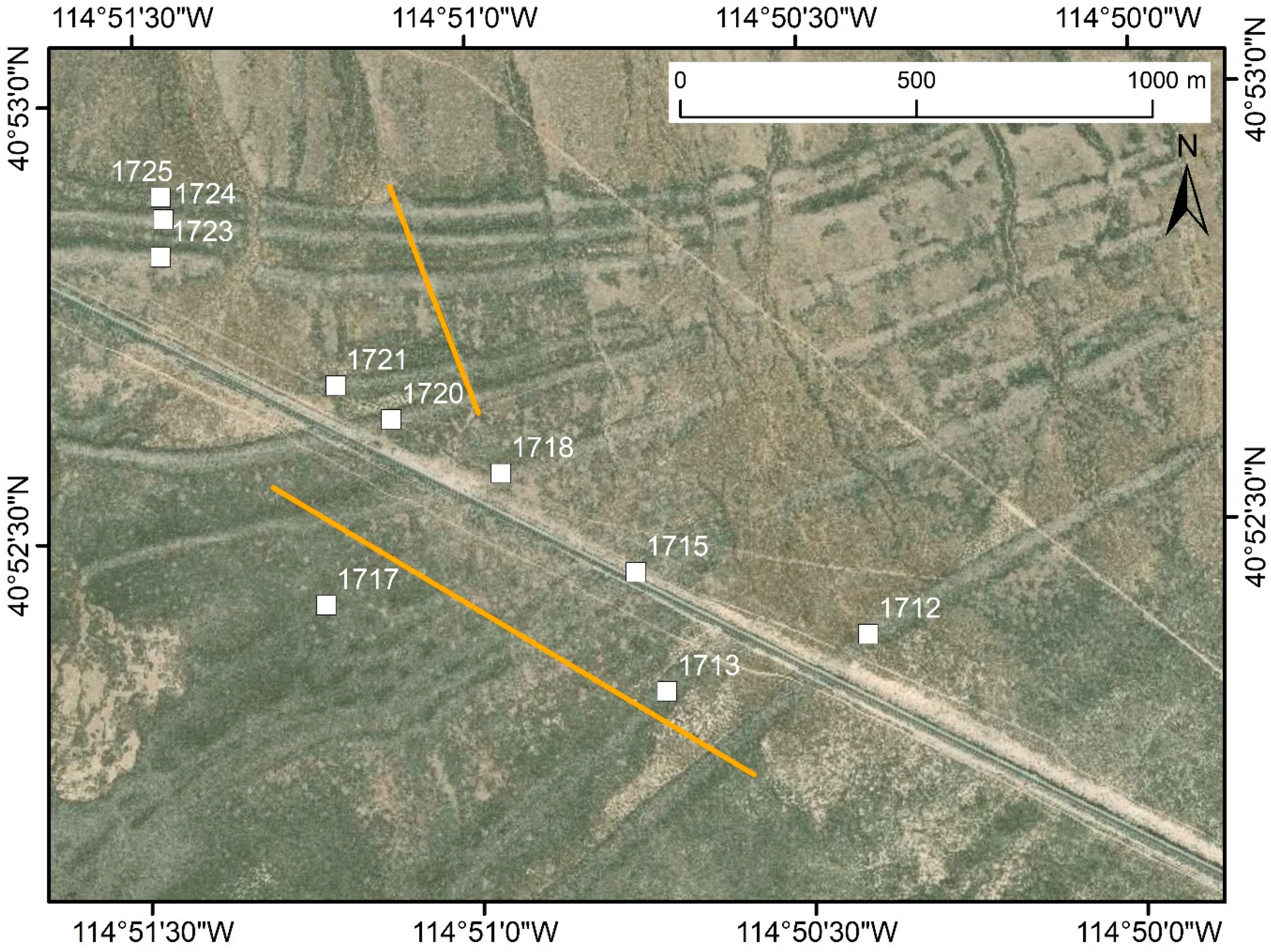
True color aerial image of the Tobar transect study area. Ten separate shoreline berms are obvious as linear features extending from the upper right to lower left. Color contrast reflects the presence of a different vegetation community on the drier, windswept crest of each ridge. The prominent line extending from upper left to lower right is the Union Pacific railroad line. White squares mark the locations of the pits excavated into each of the beach ridges. The corresponding labels indicate the reconstructed elevation of the lake surface (in meters above sea level) at the time when each ridge was constructed. The two orange lines denote the transects along which the topographic cross section (Figure 3) was measured.
Figure 2.
True color aerial image of the Tobar transect study area. Ten separate shoreline berms are obvious as linear features extending from the upper right to lower left. Color contrast reflects the presence of a different vegetation community on the drier, windswept crest of each ridge. The prominent line extending from upper left to lower right is the Union Pacific railroad line. White squares mark the locations of the pits excavated into each of the beach ridges. The corresponding labels indicate the reconstructed elevation of the lake surface (in meters above sea level) at the time when each ridge was constructed. The two orange lines denote the transects along which the topographic cross section (Figure 3) was measured.

Figure 3.
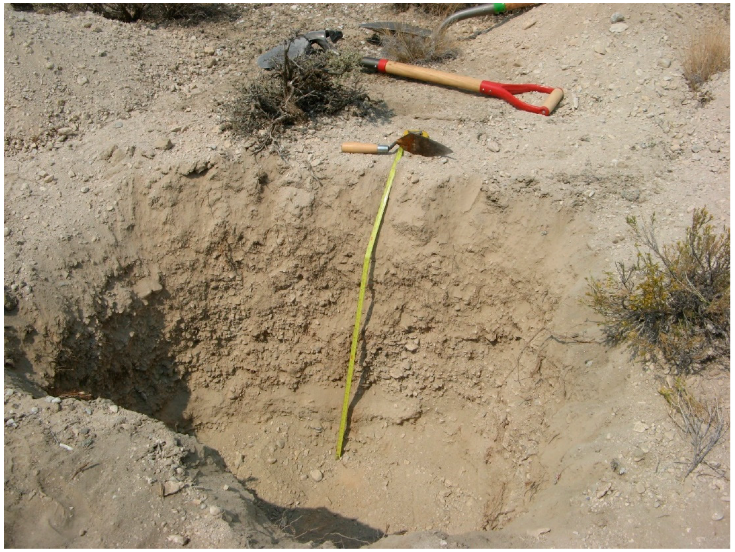
Photograph of the excavation into the 1720 m shoreline. The light-shielded luminescence sample (metal tube with black cap) is visible in a sand-rich layer near the bottom of the exposure.
Figure 3.
Photograph of the excavation into the 1720 m shoreline. The light-shielded luminescence sample (metal tube with black cap) is visible in a sand-rich layer near the bottom of the exposure.

Figure 4.
Schematic illustrating how the elevation of the shoreline berm crest relates to lake level. The still-water level is located near the center of the beach face; however, large storm waves wash up the beach face, pushing coarse sand and gravel upward to build the prominent storm berm. Particularly large waves may wash over the berm crest. The measured elevation of the berm crest, therefore, is an over-estimate of the still-water level for the lake that built each berm. In light of this, the midpoint of the beach face was considered to represent the former still-water level.

Figure 5.
Topographic profile across the beach ridges at the Tobar transect measured by a laser total station referenced to a second class 0 vertical order survey point. Berm crests are noted by red triangles and are labeled with their estimated still-water elevation, as explained in Figure 4.
Figure 5.
Topographic profile across the beach ridges at the Tobar transect measured by a laser total station referenced to a second class 0 vertical order survey point. Berm crests are noted by red triangles and are labeled with their estimated still-water elevation, as explained in Figure 4.

Figure 6.
Reconstructed hypsometry of Lake Clover. The area of the lake ranged from 740 km2 at the highstand, to 485 km2 when the lowest shoreline was constructed (blue). The rate of change from one shoreline to the next increases at lower elevations (orange).
Figure 6.
Reconstructed hypsometry of Lake Clover. The area of the lake ranged from 740 km2 at the highstand, to 485 km2 when the lowest shoreline was constructed (blue). The rate of change from one shoreline to the next increases at lower elevations (orange).

Figure 7.
Grain size distributions of samples from the Lake Clover beach ridges. (a) Samples plotted on a ternary diagram of mud/sand/gravel. Nearly all samples classify as either sandy gravel or gravelly sand. Samples 1725 is finer, classifying as a gravelly muddy sand. (b) Results of grain size analysis with laser scattering of the fine (<63 µm) fraction of the grain size samples. All samples are similar, with an overall mean of 31 µm. Samples are designated by their corresponding lake elevation, as shown in Table 1.

Figure 8.
Grain size classes in the fine fraction (<63 µm) of the samples from Lake Clover shorelines analyzed by laser scattering. Coarse silt and medium silt make up the largest proportion of these samples. Clay is relatively uncommon in the fine fraction (<5%). Samples are designated by their corresponding lake elevation, as shown in Table 1.

Figure 9.
Example exposure excavated into the crest of the shoreline built when Lake Clover stood at 1718 m. The layer of gravel-poor silt, roughly corresponding to the Av horizon, at the top of the exposure is clearly evident. Layers of imbricated gravelly sand are present below this surficial layer. A sand-dominated layer is also obvious near the bottom of the exposure.

Figure 10.
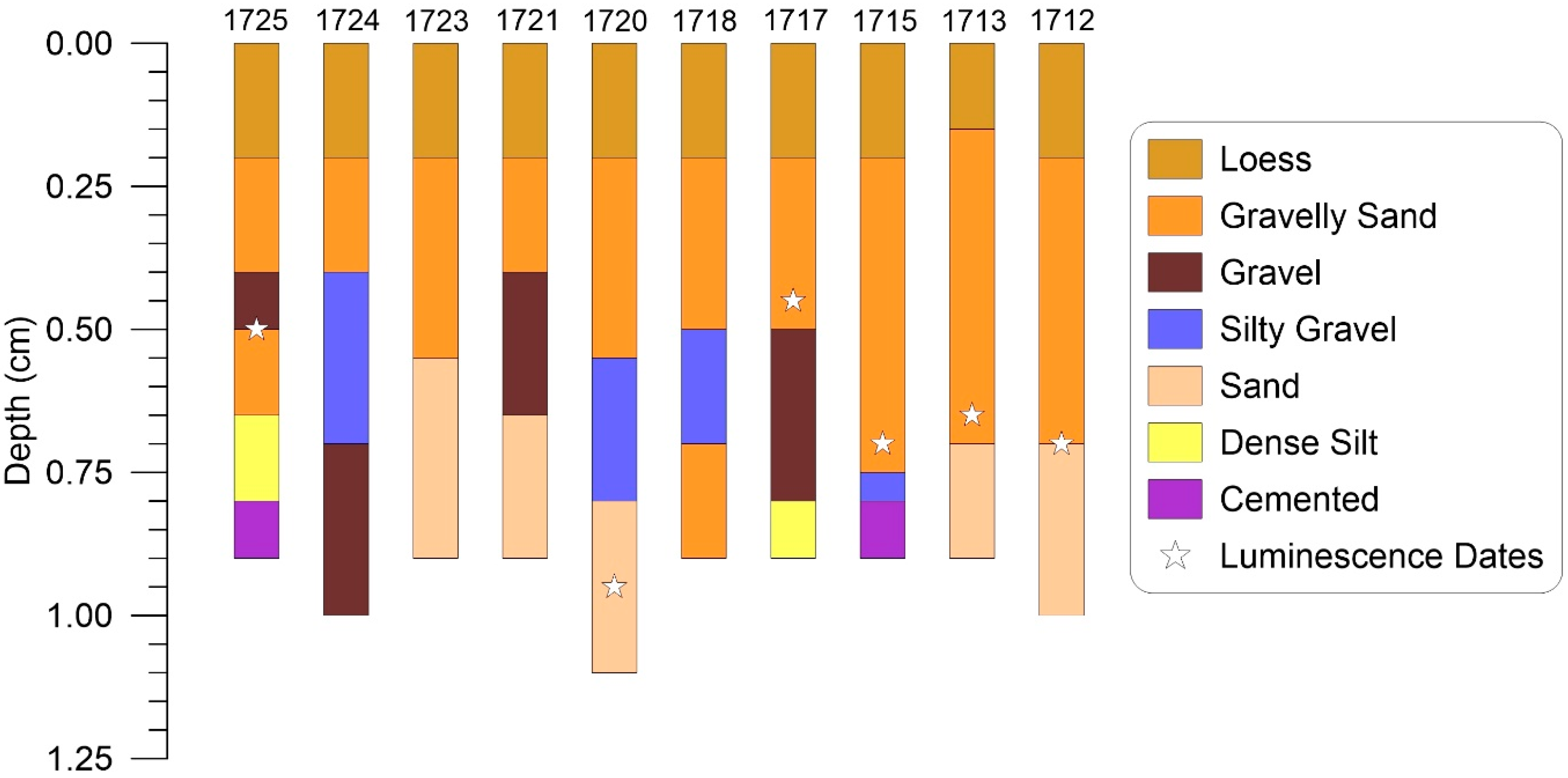
Simplified stratigraphic logs for the pits excavated into the Lake Clover shorelines, designated by their corresponding lake elevations (Table 1). All are capped by a layer of silt interpreted as loess, which overlies a gravelly sand layer. Alternations between finer (silty gravel) and coarser (gravel) sediment are present at depth. Five pits bottomed in fine sand, whereas two reached a layer of dense silt. Three excavations encountered a carbonate cemented layer. The depths of the six dated luminescence samples are shown by the stars.
Figure 10.
Simplified stratigraphic logs for the pits excavated into the Lake Clover shorelines, designated by their corresponding lake elevations (Table 1). All are capped by a layer of silt interpreted as loess, which overlies a gravelly sand layer. Alternations between finer (silty gravel) and coarser (gravel) sediment are present at depth. Five pits bottomed in fine sand, whereas two reached a layer of dense silt. Three excavations encountered a carbonate cemented layer. The depths of the six dated luminescence samples are shown by the stars.

Figure 11.
Results of luminescence dating of samples from the Lake Clover beach ridges. Ages denoted as “F” were determined with single grain analysis of K-feldspar using the pIRIR SAR protocol. The two ages denoted as “Q” were determined with the SAR protocol on quartz. “n” indicates the number of accepted discs considered in each age. Ages are presented in ka with 2-σ errors. All results were calculated using the central age model [26], shown in Table 2.

Figure 12.
Results of a comparison between pIRIR SAR and calibrated 14C ages for the highstand shoreline of Lake Clover. Gastropod shells were not encountered in the excavations at the Tobar transect (red box); however, shells from deep excavations in the highstand beach ridge at Ventosa (left photo, blue star, “V” in Figure 1, plotted in blue above), and from shallow excavations in the northeast Independence Valley (right photo, green star, “I” in Figure 1, plotted in green above) were successfully dated with 14C [14]. A luminescence sample from Ventosa (orange arrow) from a depth of ~80 cm was dated with pIRIR SAR on K-feldspar (plotted in orange above), yielding an age that matches the calibrated 14C results from the same depth in the highstand shoreline in the northeast Independence Valley. The error bars (2-sigma) on the luminescence result (PIRIR, orange above) also overlap with the 14C results from deeper within the highstand ridge at Ventosa. This correspondence lends confidence in the robustness of the luminescence age results.

Figure 13.
Luminescence-based chronology for the regression of Lake Clover. The lake reached its highstand ca. 16 ka during Heinrich Stadial I (HS-1), regressed leading into the Bølling/Allerød (B/A), built additional shorelines during or at the end of the Younger Dryas episode (YD), and constructed a final shoreline early in the Holocene after losing ~35% of its highstand area.

Figure 14.
Comparison of the hydrograph for Lake Clover (dashed black line) with other pluvial lake hydrographs for the Great Basin including Lake Franklin [13], Lake Lahonton [32], Lake Bonneville [6], Lake Surprise [31], and Lake Chewaucan [9]. A summary of lake highstands, including Lake Clover, is shown in pink [14]. Dated moraines at the Angel Lake type locality (red recalculated from [33]), and the calibrated basal 14C age for Overland Lake (star [16]) are also shown for reference.


Table 1.
Samples from the Tobar Transect.
| Sample Name | Lake Elevation | Lake Area | Relative to Maximum | Rate of Change | Sample Latitude | Sample Longitude |
|---|---|---|---|---|---|---|
| -- | (m) | (km2) | (%) | (km2/vertical m) | (degrees) | (degrees) |
| TOBAR-5665 | 1725 | 740.4 | 100.0 | -- | 40.881585 | −114.857772 |
| TOBAR-5662 | 1724 | 727.1 | 98.2 | 13.3 | 40.881158 | −114.857718 |
| TOBAR-5658 | 1723 | 712.5 | 96.2 | 14.0 | 40.880439 | −114.857809 |
| TOBAR-5650 | 1721 | 683.4 | 92.3 | 14.3 | 40.877918 | −114.853494 |
| TOBAR-5648 | 1720 | 666.8 | 90.1 | 14.7 | 40.877243 | −114.852123 |
| TOBAR-5645 | 1718 | 625.3 | 84.5 | 16.4 | 40.876165 | −114.849399 |
| TOBAR-5636 | 1717 | 605.6 | 81.8 | 16.9 | 40.873733 | −114.853863 |
| TOBAR-5630 | 1715 | 563.7 | 76.1 | 17.7 | 40.874223 | −114.846076 |
| TOBAR-5626 | 1713 | 509.4 | 68.8 | 19.3 | 40.871935 | −114.845358 |
| TOBAR-5620 | 1712 | 484.5 | 65.4 | 19.7 | 40.872932 | −114.840278 |
Table 2.
Summary of Luminescence Results.
| Sample | Lake Elevation (m) | Depth (cm) | Aliquots (nacc/ntot) | Dose Rate (Gy/ka) | 2σ (Gy/ka) | Internal Dose Rate (Gy/ka) | 2σ (Gy/ka) | Over Dispersion (%) | CAM (ka) | 2σ (ka) | MAM3 (ka) | 2σ (ka) |
|---|---|---|---|---|---|---|---|---|---|---|---|---|
| Feldspar PIRIR | ||||||||||||
| VT-3-crest | 1725 | 75 | 44/300 | 1.83 | 0.09 | 0.67 | 0.21 | 0 | 17.6 | 1.9 | 17.6 | 2.9 |
| TBR5665 | 1725 | 50 | 47/300 | 2.62 | 0.10 | 0.67 | 0.22 | 0 | 15.9 | 1.6 | 15.9 | 3.2 |
| TBR5648 | 1720 | 95 | 55/240 | 1.94 | 0.07 | 0.67 | 0.21 | 0 | 15.2 | 1.5 | 14.0 | 2.0 |
| TBR5636 | 1717 | 45 | 38/120 | 2.15 | 0.08 | 0.67 | 0.21 | 0 | 14.9 | 1.7 | 14.3 | 2.0 |
| TBR5630 | 1715 | 80 | 36/240 | 2.39 | 0.09 | 0.67 | 0.21 | 1 | 11.6 | 1.5 | 11.6 | 2.1 |
| TBR5626 | 1713 | 65 | 32/180 | 2.58 | 0.09 | 0.67 | 0.21 | 0 | 11.9 | 1.6 | 11.9 | 2.5 |
| TBR56 20 | 1712 | 70 | 32/120 | 2.76 | 0.10 | 0.67 | 0.21 | 0 | 9.5 | 1.4 | 9.5 | 2.4 |
| Quartz SAR | ||||||||||||
| TBR5665 | 1725 | 50 | 15/420 | 2.62 | 0.10 | 0.00 | NA | 28 | 16.5 | 3.4 | 11.9 | 4.9 |
| TBR5620 | 1712 | 70 | 19/600 | 2.75 | 0.10 | 0.00 | NA | 40 | 9.9 | 2.2 | 5.9 | 2.1 |
© 2020 by the authors. Licensee MDPI, Basel, Switzerland. This article is an open access article distributed under the terms and conditions of the Creative Commons Attribution (CC BY) license (http://creativecommons.org/licenses/by/4.0/).
Share and Cite
MDPI and ACS Style
Munroe, J.S.; Walcott, C.K.; Amidon, W.H.; Landis, J.D. A Top-to-Bottom Luminescence-Based Chronology for the Post-LGM Regression of a Great Basin Pluvial Lake. Quaternary 2020, 3, 11. https://0-doi-org.brum.beds.ac.uk/10.3390/quat3020011
AMA Style
Munroe JS, Walcott CK, Amidon WH, Landis JD. A Top-to-Bottom Luminescence-Based Chronology for the Post-LGM Regression of a Great Basin Pluvial Lake. Quaternary. 2020; 3(2):11. https://0-doi-org.brum.beds.ac.uk/10.3390/quat3020011
Chicago/Turabian StyleMunroe, Jeffrey S., Caleb K. Walcott, William H. Amidon, and Joshua D. Landis. 2020. "A Top-to-Bottom Luminescence-Based Chronology for the Post-LGM Regression of a Great Basin Pluvial Lake" Quaternary 3, no. 2: 11. https://0-doi-org.brum.beds.ac.uk/10.3390/quat3020011