Late-Glacial and Holocene Lake-Level Fluctuations on the Kenai Lowland, Reconstructed from Satellite-Fen Peat Deposits and Ice-Shoved Ramparts, Kenai Peninsula, Alaska

Abstract

Recent decades of warmer climate have brought drying wetlands and falling lake levels to southern Alaska. These recent changes can be placed into a longer-term context of postglacial lake-level fluctuations that include low stands that were as much as 7 m lower than present at eight lakes on the Kenai Lowland. Closed-basin lakes on the Kenai Lowland are typically ringed with old shorelines, usually as wave-cut scarps, cut several meters above modern lake levels; the scarps formed during deglaciation at 25–19 ka in a kettle moraine topography on the western Kenai Lowland. These high-water stands were followed by millennia of low stands, when closed-basin lake levels were drawn down by 5–10 m or more. Peat cores from satellite fens near or adjoining the eight closed-basin lakes show that a regional lake level rise was underway by at least 13.4 ka. At Jigsaw Lake, a detailed study of 23 pairs of overlapping sediment cores, seismic profiling, macrofossil analysis, and 58 AMS radiocarbon dates reveal rapidly rising water levels at 9–8 ka that caused large slabs of peat to slough off and sink to the lake bottom. These slabs preserve an archive of vegetation that had accumulated on a lakeshore apron exposed during the preceding drawdown period. They also preserve evidence of a brief period of lake level rise at 4.7–4.5 ka. We examined plant succession using in situ peat sequences in nine satellite fens around Jigsaw Lake that indicated increased effective moisture between 4.6 and 2.5 ka synchronous with the lake level rise. Mid- to late-Holocene lake high stands in this area are recorded by numerous ice-shoved ramparts (ISRs) along the shores. ISRs at 15 lakes show that individual ramparts typically record several shove events, separated by hundreds or thousands of years. Most ISRs date to within the last 5200 years and it is likely that older ISRs were erased by rising lake levels during the mid- to late Holocene. This study illustrates how data on vegetation changes in hydrologically coupled satellite-fen peat records can be used to constrain the water level histories in larger adjacent lakes. We suggest that this method could be more widely utilized for paleo-lake level reconstruction.

1. Introduction

Recent climate warming in the Arctic and Subarctic is well documented and is of international concern as a harbinger of the Earth’s future climate [1] (IPCC 2014). Climate records from southern Alaska, for example, closely track the climate variability of the broader North Pacific region, as reflected in indices such as the North Pacific Index (NP [2]), the Pacific Decadal Oscillation (PDO [3]) and the Aleutian Low Pressure Index (ALPI [4]). Hydroclimate, the focus of this study, is dictated by fluctuations in these key modes of North Pacific climate variability and is of increasing interest for urban water supplies, agriculture, and forestry.

On longer timescales, hydroclimate variability also bears on the global carbon budget through its impact on carbon storage in peatlands. Moisture flowing from the North Pacific has created a vast storehouse of carbon in boreal and Subarctic peatlands since the last glacial maximum (LGM) at 26.5–16 ka [5]. Recent studies have suggested, however, that postglacial moisture flow into southern Alaska did not accelerate until several thousand years after the melting of the Laurentide and Cordilleran ice sheets was well underway. Cold water persisted in the Gulf of Alaska (GOA) until the Bølling warming at 14.7 ka [6], reducing moisture flow into southern Alaska [7]. Warmer sea surface temperatures (SSTs) in the GOA and rising sea level after Meltwater Pulse 1A (14.7–13.5 ka) brought moisture into Alaska from both the GOA and the flooding Bering Sea, initiating peatland recruitment [8], major vegetation change [9], and rising lake levels (this study).

Our study presents a paleohydrological record for the central Kenai Peninsula since the end of the LGM, underscoring the impact of century- to millennial-scale modes of North Pacific variability. Water levels in closed-basin lakes (lakes with no outlets) closely reflect effective moisture (precipitation minus evapotranspiration), resulting from changes in local precipitation and evaporation from lake and soil surfaces, as well as evapotranspiration from catchment vegetation [10,11,12]. Here, we develop a record of lake-level fluctuations as a proxy for effective moisture using stratigraphic and geomorphic records, centered on Jigsaw Lake in the kettle moraine belt northeast of Sterling (Figure 1).

The Study Area

The Kenai Lowland (elevation 30–90 m asl) lies west of the Kenai Mountains (elevation 1000–1500 m asl), which form the spine of the Kenai Peninsula, separating Cook Inlet to the west from Prince William Sound (Figure 1). The mountains, comprised of Mesozoic bedrock, have experienced multiple Pleistocene and earlier glaciations. The Kenai Lowland is mantled by thick deposits left by glaciers from both the Kenai Mountains to the east and the Alaska Range to the west of Cook Inlet [21]. Glacial deposits range from highly permeable, ice-marginal sands to sandy tills, to relatively impermeable clay-rich cobble tills. A layer of fine sand- to silt-rich loess intercalated with numerous tephras mantle the uplands, ranging in thicknesses from centimeters to meters. The glaciated Kenai Lowland is underlain by flat-lying, Tertiary-age terrestrial sandstones, siltstones, shale, and coal, which are not exposed in the study area (Figure 1).

The study area is located on a rolling kettle moraine plateau (with elevations of 55 to 85 m asl) of Wisconsin age deposited during the Moosehorn stade, which reached its maximum between 23 and 19 ka [21]. This stade was by far the most extensive of the several LGM advances on the Kenai Peninsula [22,23]. At this climax of the LGM, Moosehorn ice advanced eastward from the Alaska Range, joined ice coming down Cook Inlet from the north, and extended onto the Kenai Lowland as far east as Sterling (Figure 1). A much smaller coeval advance extended westward out of the Kenai Mountains 30 km, terminating at the east side of Sterling. A 50 km-long glacial lake trending SW–NE covered today’s Moose River flats and separated the two lobes of Moosehorn ice. The eastern advance appears to have retreated without interruption, leaving few kettles on its ground moraine. The greatly extended western advance, however, left two terminal moraines, and then appears to have stagnated, leaving a jumbled, chaotic topography of eskers, kames, and kettles. This classic kettle moraine landscape shows many signs of high-water erosional activity such as wave-washed terraces, wave-cut scarps, underfit streams and steep-sided abandoned drainage channels [21]. The moraine and its surface and groundwater are drained internally by the westward-flowing Swanson River into Cook Inlet, on the western side by the south-flowing North Fork Beaver Creek (No Name Creek, local name), which drains into the Kenai River east of Kenai, and on the southeastern side by the Moose River which drains into the Kenai River at Sterling. Our eight kettle lakes are distributed across the western Moosehorn moraine, aligned in a generally east–west direction. The Moosehorn glacial stade was followed immediately by the Killey stade (19–18 ka) with the recurrence of smaller glacial advances.

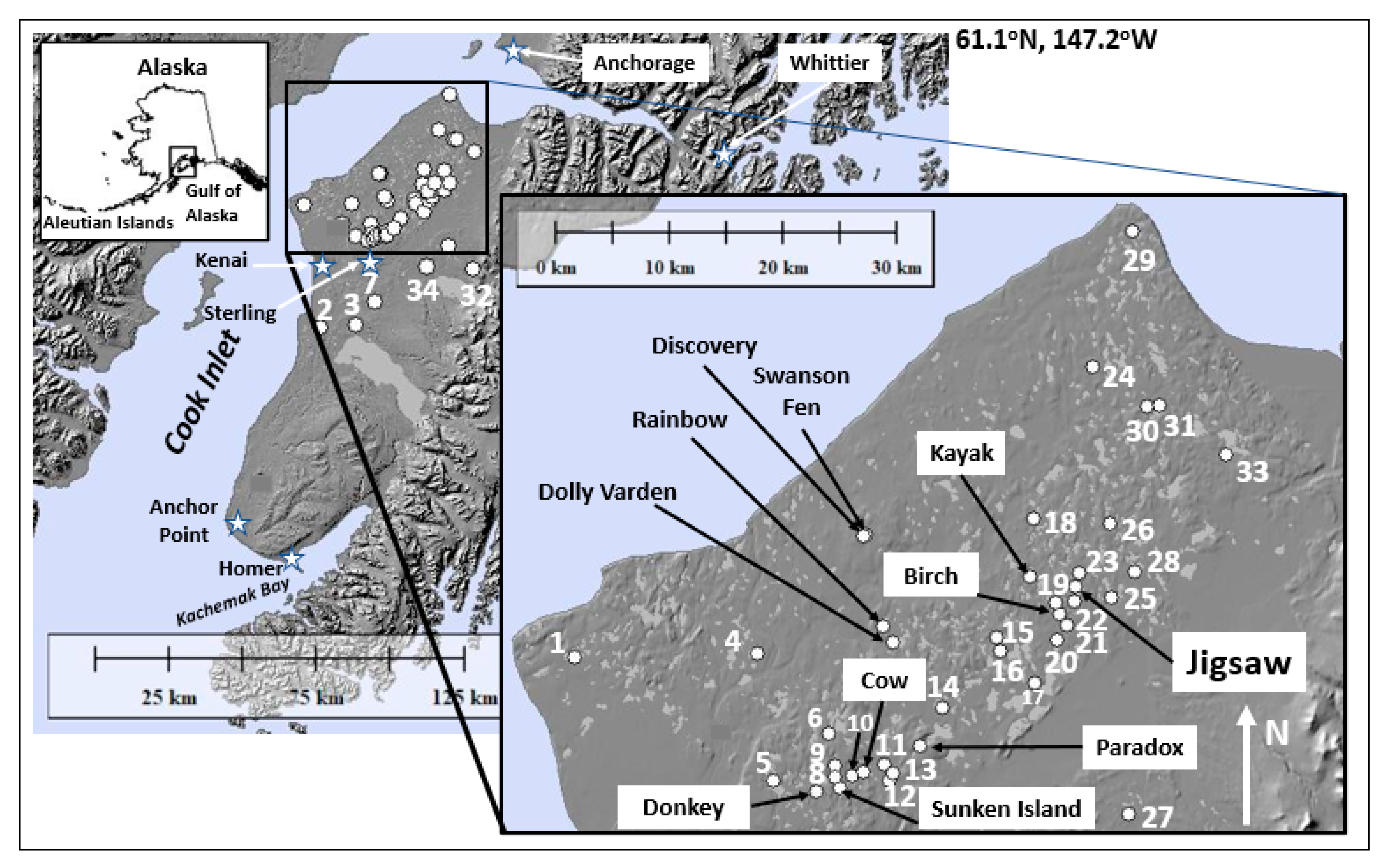
No evidence of permafrost effects, either ancient or modern, was observed in the study area, although actively degrading relict permafrost occurs in glacial lakebed wetlands of the Moose River Flats 10–15 kms east of the study area [24,25].

Jigsaw Lake, composed of four separate lobes, prompting the name “Jigsaw”, is located on a low drainage divide between the Swanson River to the north and the Moose River to the south (Figure 2). It has a relatively small catchment area (400 ha) compared to the lake itself (48 ha). Its basin is topographically closed, and ringed by a prominent wave-cut scarp at 85 m asl, 2–5 m high, and situated 2.4 m above the modern lake level.

The fact that the lake is situated at the top of its drainage divide potentially makes its water level more sensitive to variation in climatic effective moisture than lakes further down the watershed that would be buffered with groundwater flow from higher lakes [26].

The Kenai Mountains cast a strong rainshadow over the Kenai Lowland, capturing much of the precipitation coming off the Gulf of Alaska through Prince William Sound. On the windward (eastern) side of the mountains, there is heavy precipitation at Whittier (5050 mm/yr, mean annual temperature 4.4 °C) and Seward (1690 mm/yr, 4.3 °C). On the leeward side at Sterling (445 mm/yr, 1.4 °C) near our study area, and at Kenai (480 mm/yr, 1.3 °C), the climate is drier and more continental, and more similar to that of Interior Alaska [27,28].

At a regional scale, the climate of southern Alaska is driven by shifting patterns of the wintertime Aleutian Low pressure system. When the Aleutian Low pressure system is strong, it is centered over the Gulf of Alaska, and cyclonic storms frequently carry winter precipitation into south-central Alaska. With weaker Aleutian Lows, the low is elongated or splits between a west node near the western end of the Aleutian Islands and an east node in southern Prince William Sound; the west node routes winter storms toward the Alaskan Interior and the east node routes storms toward the Yukon and Southeast Alaska [4,29,30,31,32]. These shifting low pressure areas are partially tied to North Pacific sea surface temperatures described by the irregular 20 to 40 yr cycles of the Pacific Decadal Oscillation [3].

2. Materials and Methods

To document high stands of closed-basin lakes, we use two geomorphic markers—wave-cut scarps and ice-shoved ramparts—both rendered highly visible with bare-earth Light Detection and Ranging (LiDAR) imagery (Figure 3, Figures S4, S6–S8 and S10–S12). Wave-cut scarps (WCSs) are old shorelines notched into slopes around lake basins. In some places, they are only modest breaks in slope at the same elevation; in others, they are steep scarps several meters high at the top of gently sloping, wave-washed terraces surfaced with lag gravels. Ice-shoved ramparts (ISRs) on the other hand are berm deposits pushed up on the shore, either by wind-driven ice pans in the spring [33,34,35,36] or by ice expansion through a ratchet-like process of extreme cold shrinkage, ice cracking and filling with water, refreezing, and followed by rapid thermal expansion during warm periods [37,38]. On the Kenai, ISRs are often found on the west or southwest sides of lakes, where they would be formed in the spring by strong NE winds driving ice pans up on the shore (e.g., Figures S4, S6–S8, S11 and S12). On the Alaska Peninsula, local residents reported ice expansion pushing up a rampart at Telaquana Lake during the winter of 2003–2004; the disturbed shoreline spanned 275 m, with a rampart height of 1–2 m. Tipped and scarred trees suggested that this rampart was re-shoved in subsequent winters (E.E. Berg, pers. obs., July 2010). On the northern Kenai, a recent ISR of overthrust shoreline vegetative mat 0.5–1 m high was observed at Barabara Lake (E.E. Berg, pers. obs., September 2009).

To document low stands of lake level, we use stratigraphic changes registered in peat profiles from satellite fens, i.e., fens which are near or adjoining closed-basin lakes (Figure 3). Our methodology focuses on the presence or absence of terrestrial vegetation in satellite-fen peat deposits as a limit on maximum possible lake level, under the assumption that the occurrence of remnants of terrestrial vegetation, such as bryophytes and sedges, within a peat profile necessarily denotes terrestrial conditions at the lake shoreline. Our technique provides a maximum-limit estimate of lake level because the water could have been lower, but could not have been higher, for any extended period of time. Peat stratigraphy on the Kenai does not usually record episodic flooding, as such events do not cause gyttja (dark organic-rich mud) deposition or species composition change.

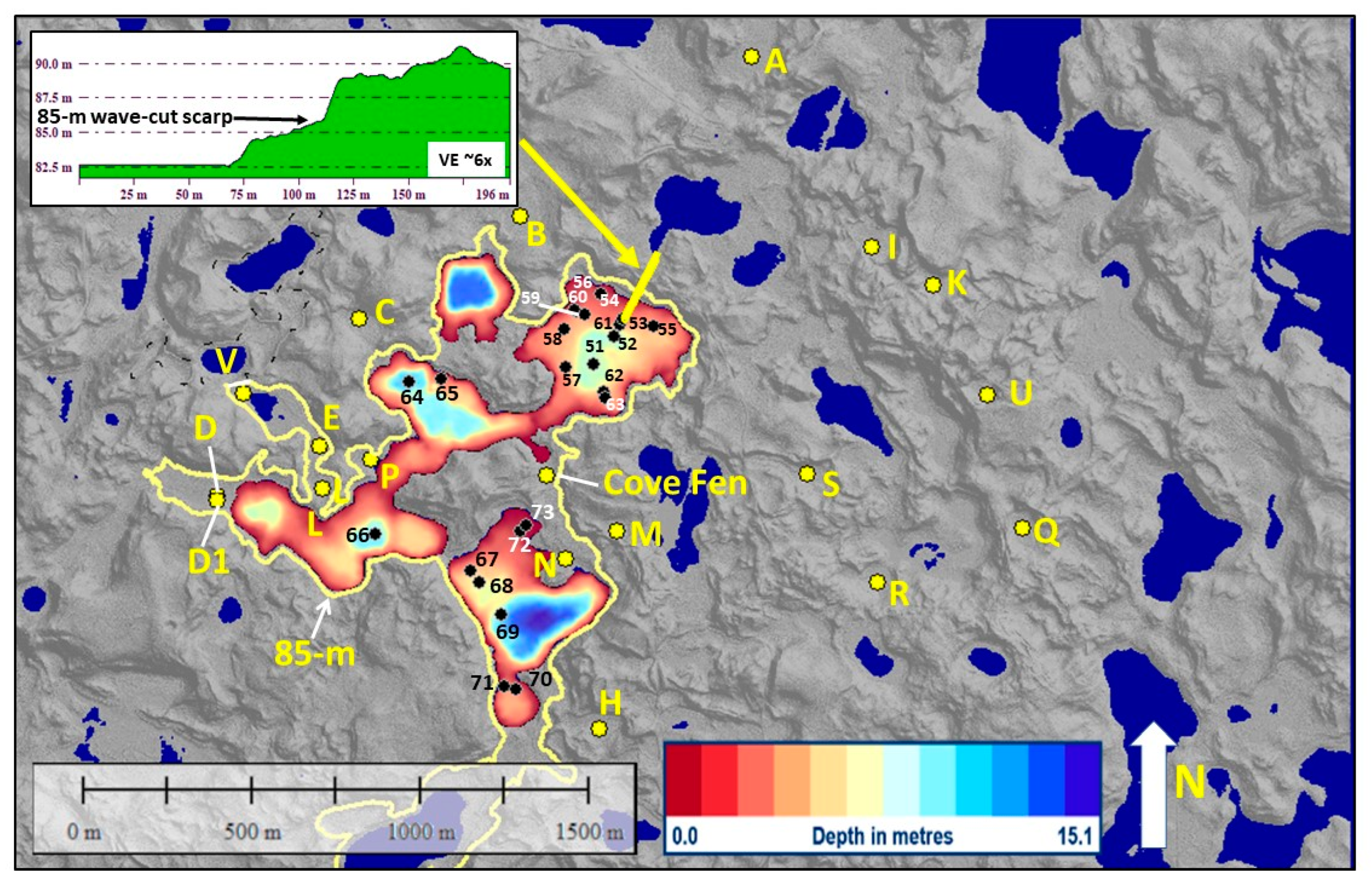
2.1. Closed-Basin Lake Aerial LiDAR Surveys

To locate closed-basin lakes, we examined Google Earth and high-resolution, bare-earth LiDAR imagery for the Kenai Lowland. The imagery was collected in May to September 2008 [39] with a vertical resolution of <30 cm and a horizontal resolution of <1 m [40]. For each lake, we used Global Mapper software to generate LiDAR topographic profiles that allowed identification of wave-cut scarps as breaks in slope at consistent elevations around the lake. We used these profiles to determine scarp heights above the modern lake level. Ponds of area <6 ha were excluded.

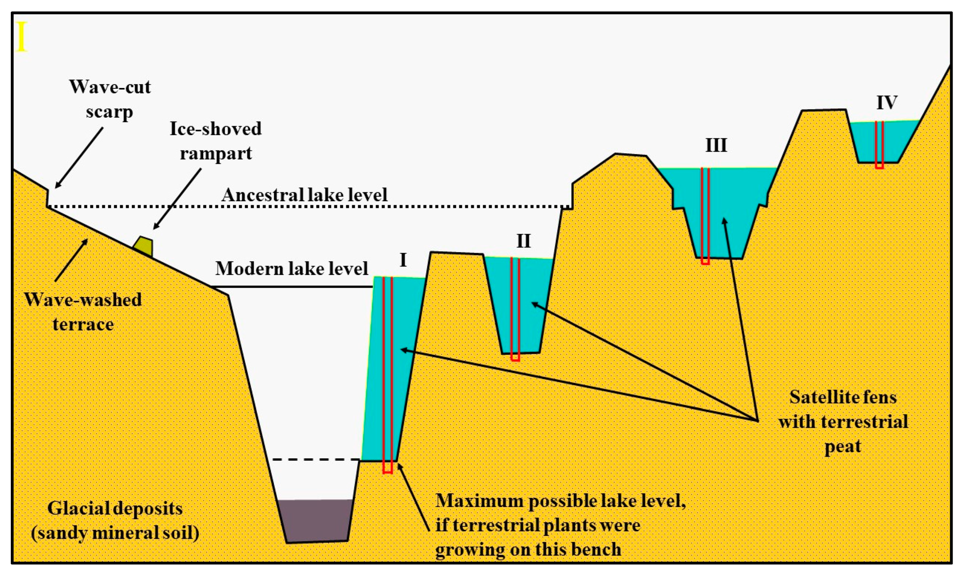
2.2. Ice-Shoved Rampart (ISR) Studies

We located ISRs on stereo aerial photos and bare-earth LiDAR, and used LiDAR profiles to measure heights of the ISR bases above modern lake levels (Figure 4, Figures S4, S6–S8, S11 and S12). We excavated trenches into the leading (landward) edges of the ramparts, described soil profiles, and collected wood and charcoal samples for radiocarbon dating. The ISR emplacement must be younger than the pre-existing organics used for ¹⁴C dating; the age of the youngest organics thus provides a limiting maximum age of the ISR formation. When we observed multiple ramparts, we excavated the most landward rampart on the assumption that it was the oldest.

2.3. Lake Sediment and Fen Peat Coring

2.3.1. Jigsaw Lake Sediment Coring

We took two initial reconnaissance cores from the two deeper basins of Jigsaw Lake with a 7.5 cm-diameter percussion corer. Following analysis of these cores, we conducted seismic acoustic and side-scan sonar profiles in all four basins to select sites for additional cores. Overlapping core pairs were located within a few meters of one another and staggered to cover breaks between core-thrust segments. The cores were taken with a 5 cm-diameter modified Livingston piston corer operated from a raft. The cores were then split, photographed, scanned for magnetic susceptibility with a Bartington field susceptibility meter, and packaged for macrofossil analysis and dating.

Two instruments were deployed to acquire three different geophysical properties. Survey lines were traveled by canoe: water depth and surface textures were recorded using a consumer-grade fish finder with side-scan sonar with dual frequency (83 and 200 kHz) for depth and a 455 kHz frequency for side imaging. The subsurface stratigraphy was acquired with a Stratbox (TM) unit which delivers a pulsed 10 kHz signal. Vertical resolution is stated as 15 cm and source velocity of 1500 m/s is assumed. The resulting proprietary recording was converted to industry standard SEGY format and processed with Sonarwiz.MAP software.

2.3.2. Jigsaw Lake Satellite-Fen and Moraine Peat Coring

To constrain paleo-lake levels, peat cores were extracted from nine satellite fens within the greater Jigsaw Lake basin, as determined by the 85 m WCS around the lake. The Cove Fen and Fens C, D, E, H, L and P (Figure 2) were sampled with a 7.5 cm-diameter Livingston piston corer, with the full cores retained for macrofossil analysis. Fens B and N were sampled with a small 2.5 cm-diameter piston corer designed to capture the lowermost 45 cm of peat above mineral soil for basal peat radiocarbon dating. The fens, here and below, were probed with a soil probe in order to core the deepest peat accessible; flooded fens were not cored in water depths >30 cm.

We took 2.5 cm cores of basal peat in the upland moraine fens around Jigsaw Lake in order to constrain the timing of LGM deglaciation in this area (Fens A, I, K, M, Q, R, S, U and V) (Figure 2).

2.3.3. Satellite-Fen Peat Coring at Regional Lakes

We took cores in satellite fens near lakes west and south of Jigsaw Lake, primarily along Swanson River and Swan Lake Roads. Full 7.5 cm diameter cores were taken at Rainbow and Dolly Varden Lakes, and basal peats were sampled with the 2.5 cm diameter corer at Birch, Cow, Dolly Varden, Donkey, Kayak, and Sunken Island Lakes (Figure 1). Core macrofossils were analyzed and radiocarbon dated.

2.4. Macrofossil Analysis

2.4.1. Macrofossil Examination

We disarticulated samples of peat in 5% aqueous KOH overnight, flushed the samples with warm water over a 150-micron sieve, and examined them in a large glass baking dish with a boom-mounted stereoscope at 7–40×. We counted large particles such as graminoid fragments and moss stems with leafy branches in the dish at 7×. For a more detailed view, we followed a modified quadrat-and-leaf-count protocol, counting the particles with a 10 × 10 mm reticle grid at 20× [41], with 5–15 randomly placed samples in the dish. We scored 20 factors, including particle counts of moss leaves by species, graminoid fragments, insect parts, percentage cover of amorphous gels, and various faunal remains. Particle counts were standardized to a uniform areal density by dividing the counts by the percentage of the grid area covered by all visible material. Gels were digitally photographed with a compound scope both with and without crossed-polarization at 40–400× to distinguish amorphous gyttja from well-humified peat that typically contained fragments of moss leaves or graminoid fibers. To describe the proportion of vascular plant material in a sample, we calculated a ratio of vascular fragments (VSWR) to the sum of vascular fragments plus moss leaves, i.e., VSWR/(moss leaves + VSWR). Macrofossil profile graphics were prepared with Tilia 1.7.14 software [42].

2.4.2. Macrofossil Interpretation

Our interpretations of peat fen environments are based on the following assumptions. Graminoids such as Carex (sedges) and Eriophorum (cottongrass) are typical early colonists on mineral soils covered with shallow water. One can see this today in wet roadside ditches filled with white cottongrass plumes; Carex rostrata s.l. is actively colonizing shallow lake edges at Jigsaw Lake after the ~1 m lake level drop of the 1990s [12] (E.E. Berg, pers. obs.). All but two of the in situ peat sequences examined in this study begin with graminoids; the two exceptions are our deepest peats—Jigsaw D1 and Dolly Varden B1, which begin with wet Drepanocladus exannulatus and wet Sphagnum species, respectively. Fens can be dominated by graminoids for thousands of years and accumulate many meters of peat if there is a generally rising water table (or rising lake level in the case of satellite fens) ([17], this study). With stable shallow water, however, we expect graminoids to be replaced by wet brown mosses (Amblystegiaceae) such as D. exannulatus (syn. Warnstorfia exannulata), as well as by wet Sphagna such as those of Sphagnum Section Cuspidata (e.g., S. riparium), Section Subsecunda (e.g., S. subsecundum) and Section Squarrosa (e.g., S. teres) [43]. Over longer periods of water level stability, we expect the emergence of the lawn-forming species of Sphagnum Section Sphagnum (especially S. magellanicum and S. papillosum) [44]. For the purposes of this study, however, the most instructive moss is Sphagnum fuscum (Sphagnum Section Acutifolia), which is the ubiquitous dry-hummock-former of circumpolar distribution [45]. The densely packed, brown hummocks of drying wetlands, such as those of the Kenai Lowland today, provide germination sites for a variety of ericaceous woody shrubs and black spruce (Picea mariana). The appearance of S. fuscum dominance in a peat core represents an increased elevation of the moss surface above the water table; this can occur either by the water table dropping or autogenically when accumulating Sphagnum reaches the limits of its water-raising capacity and only the most drought-tolerant species (i.e., S. fuscum) can survive [46]. We thus view S. fuscum as the climax species in a hydrologically stable wetland, and any conversion to wetter species must be due to a generally rising water table.

The moss Drepanocladus exannulatus (syn. Warnstorfia exannulata) is locally abundant in some of the peat cores, often in association with graminoid material and never in association with S. fuscum. The literature reports that D. exannulatus has two modes of growth: submerged and terrestrial. In the submerged mode, it can grow at extreme depths, as much as 120 m in Crater Lake [47], but more commonly to depths of 10 m [48]. In the terrestrial mode, it grows in wet wetlands, where the water table is at or near the surface. According to Glime [49] (Chapter 7–4, pp. 16–17), the leaf costa (midrib) of submerged plants extends only midway up the leaf, whereas the costa extends all the way through the tip in terrestrial plants. In our specimens, the costa always extends through the tip and forms a ridged point, indicating that the plants are basically terrestrial. In well-humified peats, the rigid points are often all that is preserved of the leaves, and we include them in the leaf counts. The co-occurrence of D. exannulatus and Sphagnum species is typically absent or only a minor element in graminoid or graminoid-Drepanocladus peats.

2.5. Testate Amoebae

The Cove Fen (Figure 2) was also sampled with a 5 cm-diameter Russian corer for testate amoebae analyses. Testate amoebae were extracted from ~2 cm³ peat samples. The samples were boiled 5 min in ~50 mL water and then filtered at 250 µm. The <250 µm fraction was left to settle overnight and the sediment fraction collected and stored in 2 mL vials with glycerol [50]. Testate amoebae were identified in wet mounts at 400× magnification with a phase-contrast microscope. We aimed for a total count of 150 individual amoebae per sample which is usually considered sufficient for ecological and palaeoecological studies [51]. Identification was based on several general keys and more detailed keys and monographs for individual genera. Past water table depths were inferred from the percentage testate amoeba data using a regional transfer function [52].

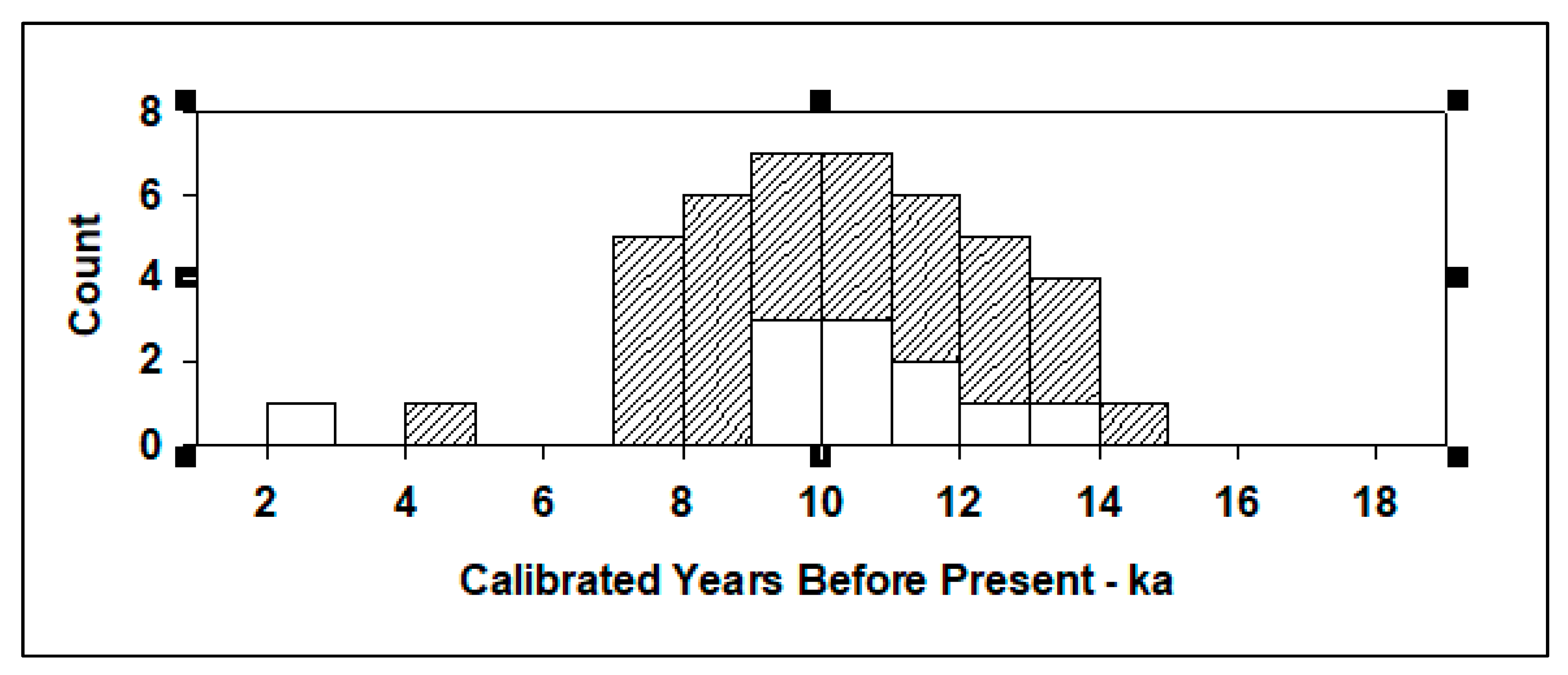
2.6. Radiocarbon Dating

AMS radiocarbon dating was performed for most samples at the Keck-CCAMS at the University of California-Irvine and Beta Analytic. All radiocarbon ages were converted to median calibrated years Before Present with CALIB 810 using INTCAL20 [53] (Table S1 of the Supplementary Materials).

3. Results

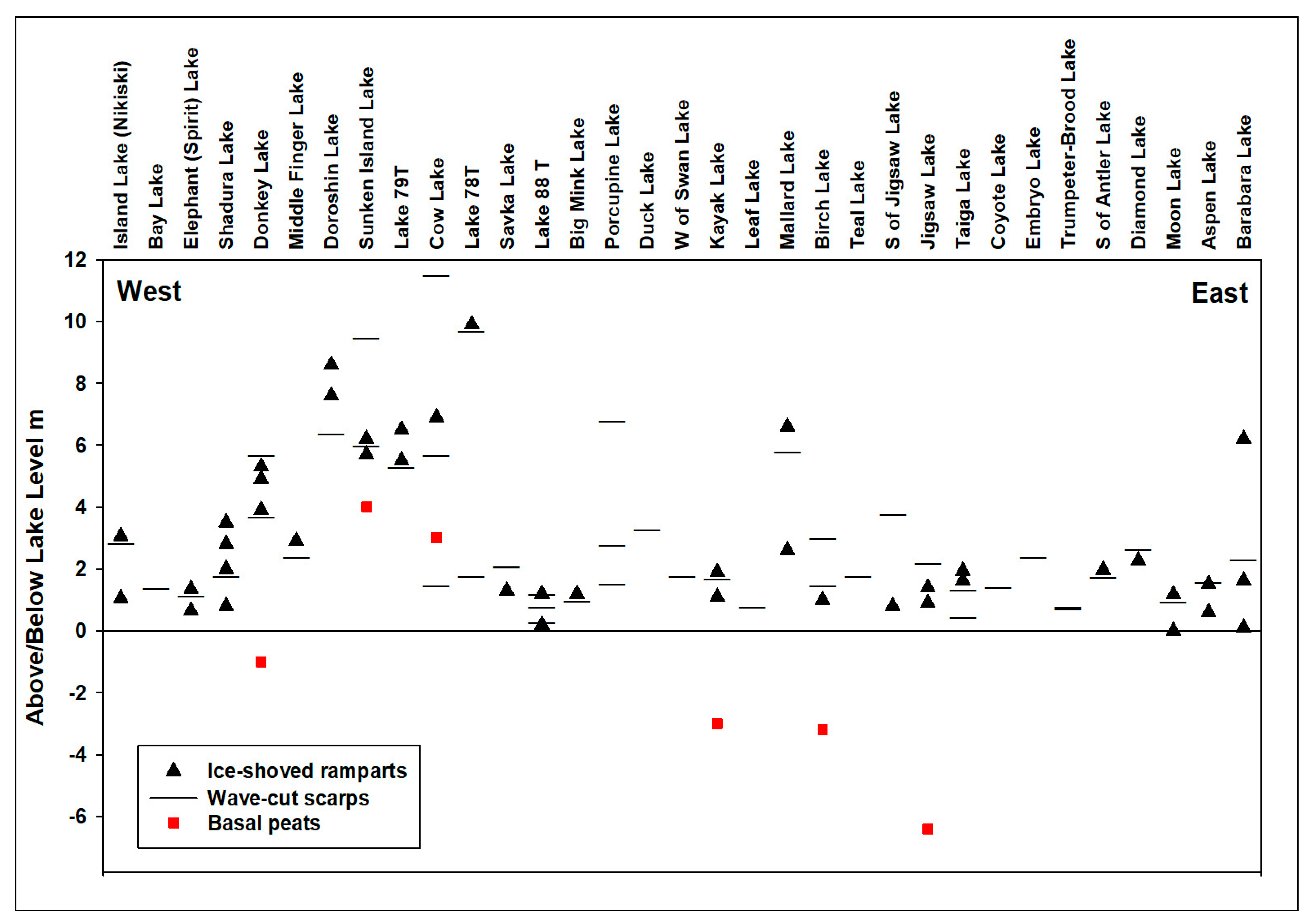
3.1. Closed-Basin Lake LiDAR Survey—Scarp Elevations

The Google Earth and bare-earth LiDAR survey revealed 33 closed-basin lakes on the kettle moraines of the Kenai Lowland. Every lake had at least one visible wave-cut scarp, with varying degrees of definition. The mean height of the highest scarps above modern lake levels was 4.1 m, with a range of 1.2–11.8 m (Figure 4). Most of the scarps fell between 60 and 90 m asl, and were probably formed on an isostatically depressed landscape; some of the variation in elevation is likely due to differences in timing and amount of postglacial land-elevation changes, as well as topographic position. We also examined open-basin lakes, many of which showed several poorly defined scarps representing pauses in outlet downcutting; others showed no evidence of scarps. A few, such as Rainbow Lake, showed prominent scarps above their present lake levels, suggesting that they were initially closed-basin lakes which subsequently overflowed and cut their modern outlets.

3.2. ISR Age and Stratigraphy

We excavated and dated ice-shoved ramparts at 15 lakes (Figure 5). On the LiDAR survey of 33 closed-basin lakes, the ISRs were situated at a mean 2.9 m (range 0–10 m, n = 39) above the modern lake levels. Close examination of the contorted stratigraphies and multiple radiocarbon dates revealed that many ramparts were formed by multiple episodic shoving events widely separated in time (Figure 5, Figures S5 and S9). The closed-basin lake ISRs mostly dated to <5.2 ka. At Pollard Lake, the most landward (and presumably oldest) of a nested set of five ramparts dated to 11.2 ka; this is an open-basin lake in a meander cutoff from the Kasilof River in an entirely different geomorphic setting than the closed-basin kettle lakes. At Pollard Lake, a satellite-fen basal peat dated to 14.2 ka, which implies that the fen was flooded at least episodically during subsequent events of ISR formation (Figure 1).

3.2.1. Jigsaw Lake Sediment Coring

Seismic profiles showed evidence of slumping and normal faulting along the steeper basin edges, especially in the NE basin of Jigsaw Lake, which was surveyed in the most detail (Figure S1 [54]). The side-scan sonar showed a gravelly slope, suggesting exposed glacial till with a slump deposit at its base (not shown).

Ten pairs of lake sediment cores revealed 15 peat layers of limited horizontal extents. Several of the peats were clearly detrital, as indicated by plant fragments in a sandy matrix, but most had normal horizontal bedding, with no sand. Nine of the fifteen peat layers had chronologies in stratigraphic order, whereas five exhibited age reversals, three of which were significant at the 95% level (#52B, 55, and DK 2001). The cores typically terminated at sharp contacts in silt, sand or sandy to gravelly glacial till. None of the lower peat layers was underlain by gyttja, although gyttja was usually found on top of peat layers and extended to the modern sediment–water interface.

We present three examples of core stratigraphy in Figure S2 of the Supplementary Materials to illustrate the interpreted sequences.

3.2.2. Jigsaw Lake Satellite-Fen and Moraine Peat Coring

The stratigraphy of the Cove Fen core is typical of the Jigsaw Lake fen peats and was sampled at the highest resolution (Figure 6). The basal peat is highly humified graminoid peat containing abundant Carex perigynia and cladoceran carapaces. At 7.9 ka, it transitions to Sphagnum fuscum with only a trace of graminoids. At 4.8 ka, graminoids return, supplemented with Sphagnum Sections Sphagnum and Subsecunda. The depth-to-water (DTW) chronology reconstructed from the testate amoebae profiles in the core show that the water table was generally approximately 30 cm below the fen vegetation surface, with two more humified layers indicating somewhat drier periods at ~3 and 4 ka (Figure 6). The detailed profile of taxa does not show any evidence (such as gyttja or silt) that the fen ever flooded (Figure S3).

Fen D-D1 is the deepest peat recovered at Jigsaw Lake (Figure 7). The basal section is Drepanocladus exannulatus peat with a trace of graminoid (Carex) dating to 11.3 ka, followed by Sphagnum Section Cuspidata. Sphagnum fuscum appears above this, along with Calliergon stramineum and more graminoids. At ~10 ka, the peat transitions to essentially pure graminoids. At ~8.2 ka, Sphagnum Section Cuspidata appears in addition to the graminoids; by ~7 ka, the peat is dominated by Sphagnum Section Sphagnum, which gives way by 4 ka to graminoids and Sphagnum Section Cuspidata, with the graminoids disappearing at the top of the section. Two cores were taken at this site within a few meters of each: macrofossil analysis and six radiocarbon dates were obtained on the first core (D), with a basal date of 11.2 ka. The second core D1 was 0.9 m deeper, with a basal date of 11.3 ka.

The Jigsaw Lake fen peats are summarized in a topographical profile in Figure 8.

Peat core sections from satellite fens are arranged clockwise around the lake from west to east. Green overlay shows wet fen conditions, brown overlay shows drier fen conditions. Maximum lake levels are estimated from the Fen D trajectory in Figure 9. Dotted lines show two important isochrons: 9.2 ka when lake level rise slows from the early rapid rise period, and 4.8 ka when the Cove Fen begins to flood and shift back to wetter vegetation. All cores terminated in mineral soil; basal dates are shown at the core bottoms. The variation in fen elevations is simply due to the kettle moraine topography upon which these fens are perched (Figure 2); no trend should be interpreted from the horizontal arrangement of the cores in the graphic.

The upland kettle fens around Jigsaw Lake yielded basal peats composed of moderately to well-humified graminoids, Sphagnum sp. and Drepanocladus exannulatus, with ages mostly in the range of 14–9 ka (n = 11). The lake satellite fens were mostly in the 14–7 ka range (n = 32) (Figure 10, Table S1 of the Supplementary Materials).

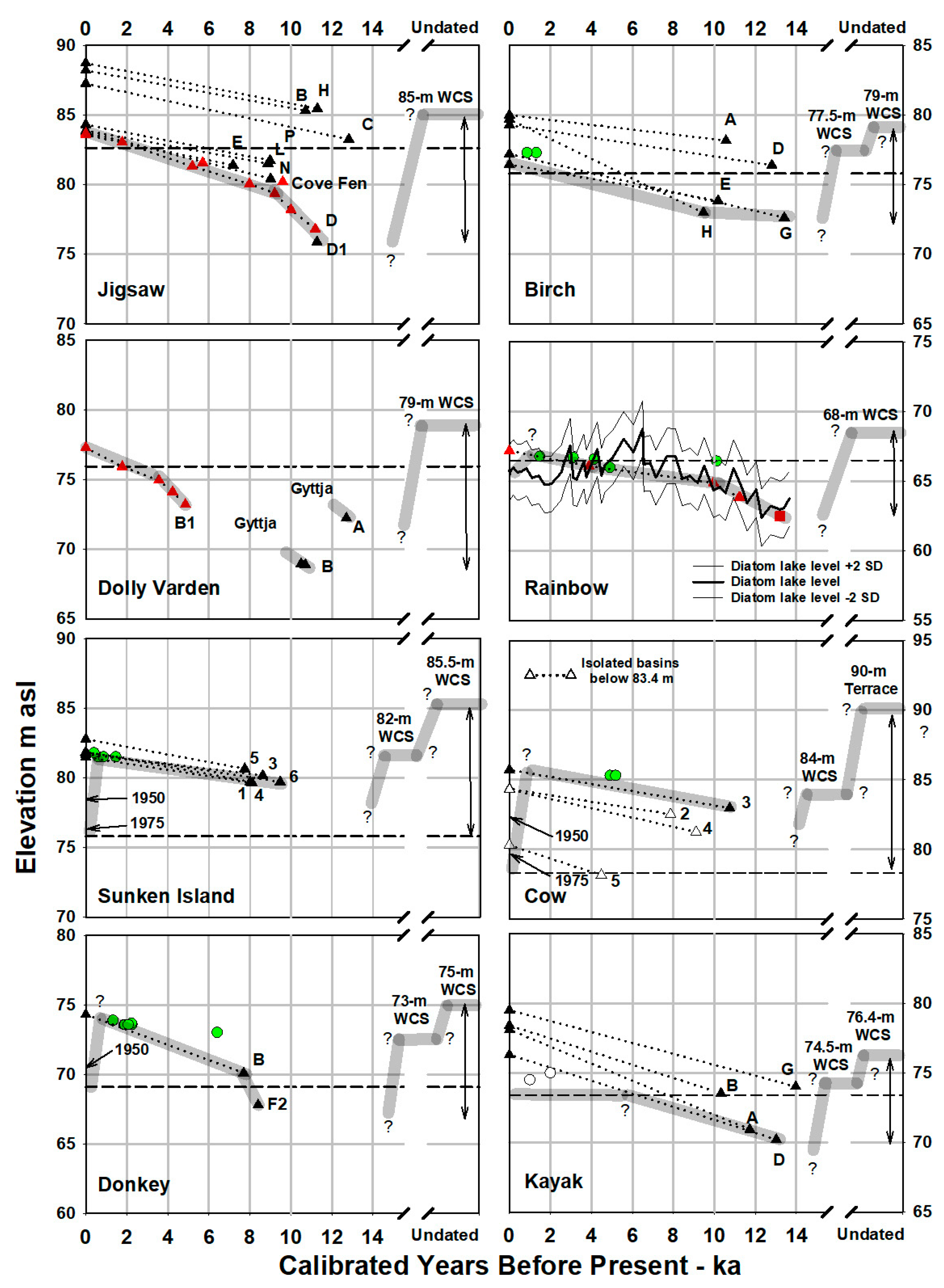
3.2.3. Satellite-Fen Peat Coring at Regional Lakes

The fens of Jigsaw Lake provided a detailed history of a single ancestral lake basin, with hydroclimate variability appearing to play a major role. We sampled fens at seven other lakes in the area to see if they shared similar histories and climatic sensitivity. Jigsaw Lake does not have well-developed ISRs, whereas ISRs are prominent features at many lakes on this kettle moraine landscape. We thus added lakes with strong ISRs to see what additional information they might add to the climate narrative. We took full-length 7.5 cm cores at Rainbow and Dolly Varden Lakes, and 2.5 cm basal cores at Birch, Kayak, Cow, Sunken Island, and Donkey Lakes (Figure 1, Table S2 of the Supplementary Materials). These cores reinforce the more comprehensive work at Jigsaw Lake, but also provide some striking differences.

Rainbow Lake (Figure 11 and Figure S8) The lake is ringed by a discontinuous WCS at 68 m asl, which is locally quite steep, indicating a long period of high lake level stability at that level. The lake appears to have been a closed basin during the scarp-forming period, although it now has a narrow outlet at 66 m asl. The constricted morphology of this narrow outlet suggests a recent formation. The present lake level of 66.5 m asl is now controlled by a road culvert in the outlet channel. Peat accumulation at our coring site initiated at 11.2 ka with a 3.5 m-thick interval of peat composed primarily of graminoids (Carex and Eriophorum), except for a major shift in the uppermost 50 cm to Sphagnum species, dominated by S. girgensohnii near the surface. Several ISRs dating from 10.1 to 1.5 ka are emplaced 1–2 m below the scarp on the west side of the lake (Figures S8 and S9).

Dolly Varden Lake (Figure 11 and Figure S10) Geomorphic features around Dolly Varden are not as clearly defined as at the other lakes. A wave-cut scarp is weakly traceable around the lake, but probably does not represent a long period of lake level stability. The lake appears to drain north toward the Swanson River through a heavily vegetated wetland, but there is no visible channel. The fact that the lake level has not dropped in recent decades, unlike the obviously closed-basin lakes in this area, implies that its level is controlled by outflow, however small that might be. The shoreline has a steep wave-eroded scarp of ~1 m high. There are minor (<1 m) ISRs capping some of the scarp; these could have been formed by extreme ice push-up events and do not necessarily indicate higher lake levels. We found no ISRs set back a distance from the present shoreline at higher elevations, such as we see at many closed-basin lakes.

At Fen A, the 2.5 cm core revealed a coarse basal fibrous peat >32 cm thick at a depth of 4 m, dating to 12.8 ka and overlain by gyttja. At Fen B, the 8.5 m section begins with gyttja, followed by 15 cm of peat composed of Section Sphagnum (S. magellanicum), Drepanocladus exannulatus, Amblystegium cf. riparium and minor graminoids dating to 10.7 ka. The next 4 m of the core is entirely gyttja, and the upper 4 m is graminoid-Sphagnum Section Sphagnum peat dating from 4.9 ka. These cores are unique in this study by containing the presence of gyttja in satellite-fen peats.

Birch Lake (Figure 11 and Figure S12) Birch Lake is ~2 km SW of Jigsaw Lake; it is 6.8 m lower in elevation and possibly receives an input of ground water from Jigsaw Lake through the sandy till. The lake has WCSs located at 79.0 and 77.5 m asl, with a modern lake elevation of 75.8 m asl. The ancestral 77.5 m asl lake level is represented by several flat, wave-washed islands and beaches on the western and northern sides of the lake that support several small (0.3–0.6 m) ISRs, as well as a prominent 1 m-high ISR which was formed by two shove events at 1.3 and 0.9 ka. We took 2.5 cm basal cores at 5 satellite fens, all of which contained bryophyte-dominated basal peats. Fen G with a basal date of 13.4 ka is the oldest satellite fen in our study.

Kayak Lake (Figure 11 and Figure S11) Kayak Lake is ringed with two distinct WSCs at 74.5 and 76.4 m asl. Two ISRs (undated) are visible on the LiDAR at the south end of the lake. At 75.0 m asl, ISR-1 is sharply defined (3 m high and 20 m wide); such a delicate feature must mark a transient highest-level stand, as it would not survive wave attack. The smaller and somewhat lower ISR-2 at 74.5 m asl records a younger high stand. We took 2.5 cm basal cores at three satellite fens: Fens A and B showed basal Drepanocladus exannulatus peat, with no Sphagnum or graminoids, and Fen D (oldest) showed moss and graminoid basal peat dating to 13 ka.

Cow Lake (Figure 11 and Figure S7) Cow Lake is ringed by a prominent WCS at 84 m asl. Two broad, wave-washed terraces on the east and NE sides of the lake record an earlier high water stand at 90 m. Cow Lake has only one satellite fen (Fen 3) near the lake, which is isolated from the lake by an undated ISR at 85 m; a 2.5 cm basal peat core dated at 10.7 ka in this fen. We sampled three fens whose bottoms lie within (but below) the 84 m asl scarp; they all would have been isolated from the lake when the lake fell below ~84 m asl (Fen 2 at <86 m, Fens 4 and 5 at <83.5 m, as in Figure 3, Fen III). Two ISRs extend intermittently for 0.5 km along the west side of the lake, locally pushed up against the WCS, which can be 4–5 m high and quite steep; a thrust event of older sediments (5.2 ka) over younger sediments (4.9 ka) was dated in the larger, landward ISR.

Sunken Island Lake (Figure 11 and Figure S4) This lake is ringed with a prominent WCS at 82 m asl. A broad wave-washed terrace on the west side of the lake at elevation 85.5 m asl records an earlier high-water stand. A 1400 m fortification-like ISR wraps around the western embayment of the lake, being 0.5–2 m in height and 3–7 m in width. It is mostly continuous along the upper margin of the wave-washed terrace, as much as 120 m back from the lake shore, and is pushed up against the steep WCS on the northern side (Figure S4). Basal peats were sampled with 2.5 cm cores in five fens; the lowest three with elevations at ~79.5 m asl dated from 9.5 to 8 ka (Fens 1, 4 and 6). Fens 3 and 5 were <1 m higher and dated to 8.6 and 7.7 ka, respectively. We dated three ice-thrust events at the south end of the rampart (ISR-2) at 1.47, 0.59, and 0.86 ka (bottom to top), with the dates indicating that older material (0.86 ka BP) was thrust over younger material (0.59 ka). A sample from the NW corner of the rampart (ISR-1) dated at 0.40 ka.

Donkey Lake (Figure 11 and Figure S6) The lake is ringed by a strongly defined WCS at 75 m asl and an even more strongly defined younger WSC at 73 m. A 375 m ISR (~1 m high) runs along the SW side of the lake, on top of the 73 m surface; we obtained seven radiocarbon dates in a soil profile at one site, which revealed at least four thrust events dating from ~6.4 to 1.3 ka. Fen B is separated from the lake by a 2 m-high ISR (undated) at 73 m asl. Peat samples were recovered with the 2.5 cm corer in Fen F2 at a depth of 2.7 m (but not reaching mineral soil) showing well-humified Drepanocladus exannulatus peat dating to 8.4 ka.

To summarize, the seven lakes described above, as well as Jigsaw Lake, all show the wave-cut scarps of their ancestral lake basins. The lake levels generally rose throughout the Holocene from late-glacial low stands; only Dolly Varden shows clear evidence of pauses in this advance, at 10.7 and 4.9 ka. Six of the lakes show prominent ISRs, mostly dating at <2.4 ka (Figure 5).

4. Discussion

We summarize our interpretations of the presented data, and then lay out an overall narrative for the hydrological history of the Kenai Lowland after the LGM.

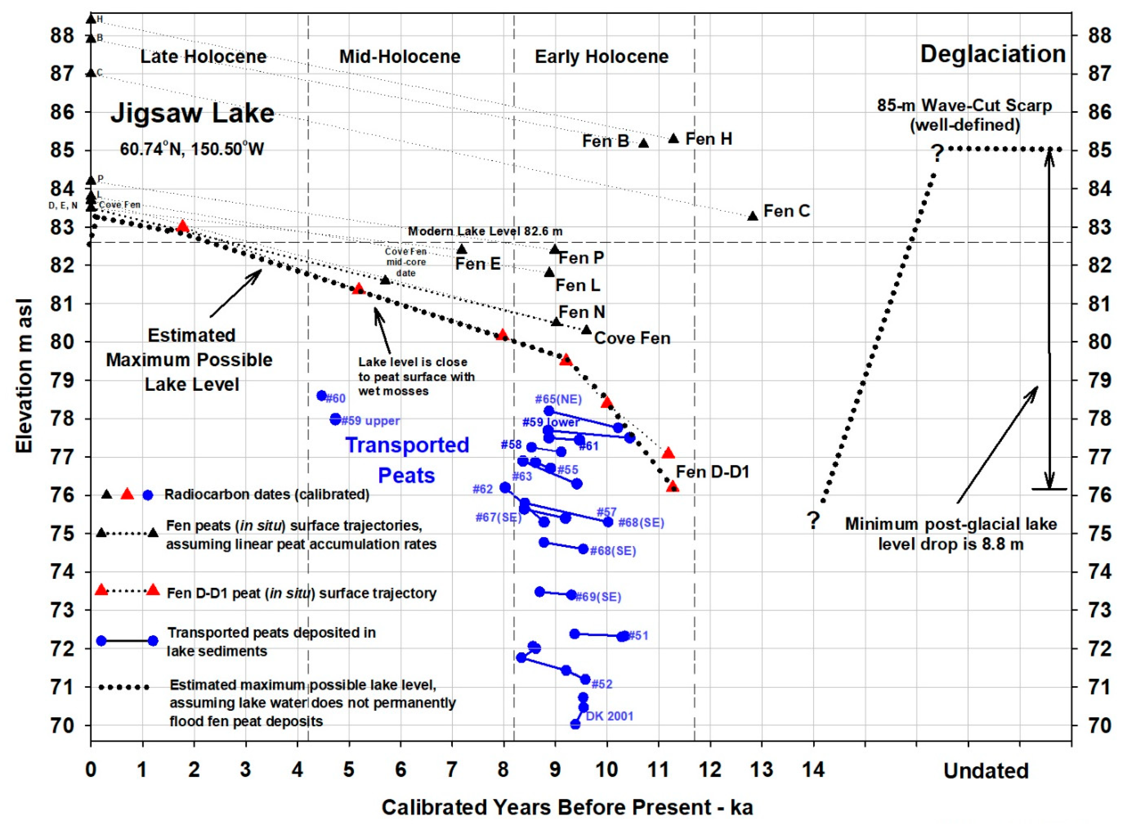
4.1. Jigsaw Lake Transported Peats

The multiple, discontinuous peat layers in Jigsaw Lake appear to be transported slabs. That these peats are not in situ is clearly indicated by slumped lake sediments in the seismic profiles and core stratigraphy that includes heavily fragmented peat textures, inverted dates, and sharp juxtaposition of unhumified plants and well-humified peats. The peats initially began accumulating prior to 10.4 ka on the lake shore apron that became exposed when the lake level had fallen almost 9 m below the 85 m asl wave-cut scarp. The peats were undercut by a rising lake level beginning approximately 9.2 ka (as shown by sloughed peat in cores #51 and DK 2001) and continued to slough off until 8 ka. A second period of rising lake level occurred approximately 4.5 ka and displaced more peat (cores #59 Upper (Figure S2) and #60) (Figure 9).

The satellite fens around Jigsaw Lake began accumulating peat during the initial lake level rise, i.e., 11 to 9 ka, even though they were perched several meters higher than the lake level and hence were not hydrologically connected to the lake at that time (Figure 9).

4.2. Jigsaw Lake Satellite-Fen Peat Coring

Fen D-D1 (Figure 7, Figure 8 and Figure 10) has the deepest and most complete record of lake level rise at Jigsaw Lake. We interpret the lowest peat as a classic wet-to-dry sequence, starting with D. exannulatus growing at the lake water edge. Somewhat drier Sphagnum Sect. Cuspidata appears next, and is succeeded by dry S. fuscum and Calliergon stramineum, a generalist moss that can be found in both wet and dry habitats. This initial wet-to-dry sequence plausibly represents autogenic succession [55], as the fen surface has by now (~9.8 ka) grown an additional 1 m above its original water table; alternatively, the wet-to-dry shift may correlate with an interval of low stand at Dolly Varden Lake (Site B, discussed below). Wet conditions returned to satellite-fen D-D1 at the 400 cm depth (8 ka), with Sphagnum Section Cuspidata and the appearance of cladoceran carapaces; conditions remain wet through the remainder of the core. This upper sequence suggests, first, that the lake level has risen substantially and has nearly caught up with the Sphagnum surface at 8 ka, and second, that the rising peat surface generally tracks the rising lake level after 8 ka.

The full set of Jigsaw Lake fen peats is displayed in an elevation transect around the lake (Figure 8). The earliest vegetation in all the fens was composed of graminoids in shallow water, which then transitioned into dry Sphagnum fuscum. This transition is consistent with both autogenic succession and a mid-Holocene dry period (discussed below). Indications of wetter conditions subsequently appear in all the fens, albeit idiosyncratically, at times ranging from 4.8 ka (Cove Fen) to ~3.3 ka (Fens E, P & C); Fen H (the highest) shifts to somewhat wetter conditions at 7.2 ka but still retains S. fuscum thereafter, mixed with graminoids. We interpret these time-transgressive dry-to-wet transitions as responses to a wetter late-Holocene climate, strongly modified by local site geomorphic and vegetation conditions.

The initial onset of peat accumulation was likely to have been strongly conditioned by local factors. The peat recorders, so to speak, are turned on in these fens over a wide time span, from 11.3 to 7.2 ka; regionally the span is even greater, from 14.2 ka (Swanson Fen) to 8.2 ka (Donkey Lake) (Figure 12). There could be at least three explanations for these differences; first, foundered ice blocks of different size and burial depths could melt out at quite different times in this intensely kettled topography [56]. In north-central Wisconsin buried Wisconsin-age ice persisted at least 5000 years after retreat of the active ice [57]. Second, peat accumulation requires an effective moisture high enough that the rate of vegetative accumulation exceeds the rate of decomposition. If the moisture regime fluctuates sufficiently, accumulated peat, unlike lake sediments, can be lost to decomposition or wildfire. Third, topographic relief on the substrate can allow peat to accumulate in low spots long before higher areas, so that multiple cores in the same peatland exhibit a several-thousand-year range of basal dates [58]. Differentiating among these factors is difficult, but not necessary for this study; once the peat recorders are turned on, their hydrological records are independent of the starting date. Additionally, once turned on, the great water-holding capacity of (especially Sphagnum) peat tends to promote the accumulation of additional peat.

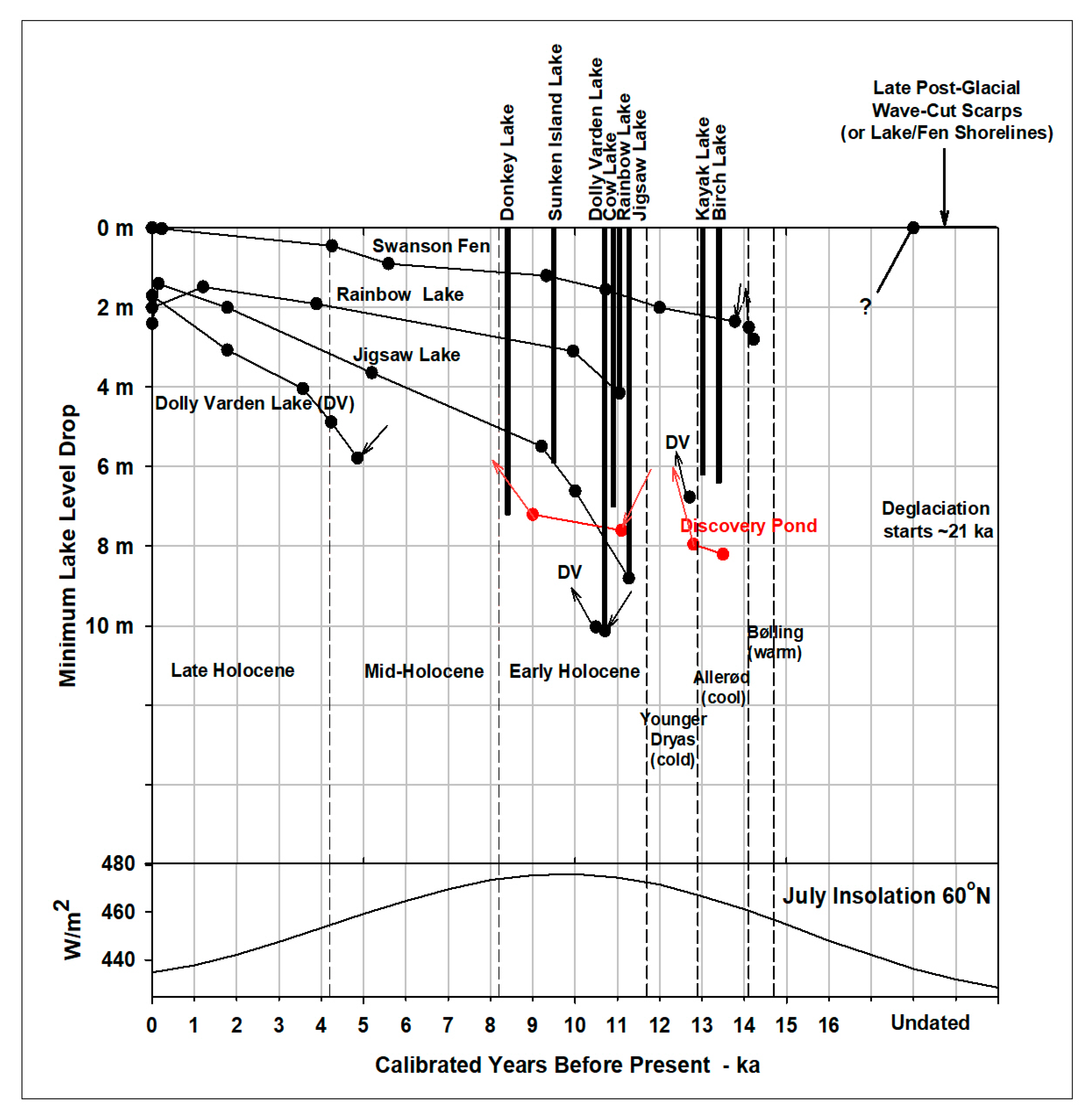
4.3. Reconstructed Water Level Changes

We summarize water level changes in the regional lakes with a series of interpretive hydrographs showing the lake level chronologies as constrained by erosional features (wave-cut scarps and wave-washed terraces), terrestrial fen peats, and ice-shoved-ramparts (Figure 11). The hydrographs are superposed in a composite graphic with data from the literature (Figure 12). Seven distinct phases of lake level history emerge out of this synthesis: (1) An initial wave-cut scarp-forming period, (2) a falling lake level period culminating in the lowest stands, (3) initial rising lake levels 15 to 11 ka, (4) early Holocene rising lake levels (first rapidly, then more slowly), (5) a mid-Holocene period of relatively dry conditions, (6) a late-Holocene period of still higher lake levels, (7) culminating in late 20th century declines.

(1) The WCS-forming period (21 to 19 ka). Our lake chronologies begin with the erosion of high-level shorelines of the ancestral lakes that first formed in these basins during the last major deglaciation. The lakes originated as part of a large kettle field that formed as rising temperature caused the stagnation and downwasting of a glacier that had advanced onto the Kenai Peninsula from across Cook Inlet. Buried ice was likely still present in many kettles at ~19 ka when waves began cutting scarps along lakeshores. The steepness of the WCSs indicates considerable fetch for wind-driven waves, which could not effectively be generated until most of the remnant glacial ice had cleared from the lake basins.

Although we have not been able to directly date wave-cut scarps, we hypothesize that the scarp-forming period coincides with the final stages of Moosehorn (late MIS 2) deglaciation. Our earliest dates for deglaciation on the Kenai Lowland (21–19 ka) are from cosmogenic exposure dating of glacially transported granitic boulders near the study area [62].

Modeling of southern Alaska climate at the terminal LGM (21 ka) suggests that summers were warmer, and that the AL was stronger in winter than it is today [63,64]. A strong AL would advect moist winter air into southern Alaska from the Gulf of Alaska (GOA) [4], providing snowfall for the Moosehorn ice sheets. Warm summers, however, would ultimately lead to melting these ice sheets.

(2) Fallinglake level period (19 to 15 ka). Evidence of falling lake levels is represented by the shoulder aprons around closed-basin lakes. These aprons extend downward from the WCS shorelines, passing below modern lake levels to the depths of the adjoining satellite fens with terrestrial peat deposits. For example, at Jigsaw Lake, the falling period is represented by the slope that extends downward from 85 m asl scarp to 76 m asl (to the bottom of the yellow zone in Figure 2). This lake level decline opened up 70% of the ancestral lake basin to vegetative colonization. Similar declines of 4 to 10 m occurred in all eight lakes examined and are one of the most striking features of these lake geomorphologies and their hydrological histories (Figure 11).

We suspect that these declines reflect a millennial-scale epoch of aridity in southern Alaska, caused by a cold SSTs in the GOA during the deglacial period. Sediment cores taken in the GOA and along the British Columbia coast show that NE Pacific waters were 4–5 °C colder between 19 and 14.7 ka than the early Holocene [6]. These authors propose that SSTs fell in response to repeated deliveries of freshwater from Columbia River outburst floods, sourced from glacial Lake Missoula, as well as by meltwater from coastal glaciers. According to [7], the late-glacial midlatitude jet stream carried North Pacific moisture into southwestern North America and supported large pluvial lakes, such as Lake Bonneville in Utah, leaving the Pacific Northwest relatively depauperate in moisture. At 14.7 ka, however, modeling by these authors suggests an abrupt reorganization of this circulation, starting with major melting of the Cordilleran and Laurentide icesheets, warming of the GOA SSTs, and shifting of moisture flow northward into the Pacific Northwest and southern Alaska.

(3) Initial rising lake levels (15 to 11 ka). By 14+ ka, the fen “peat recorders” were turned on, and lake levels had already risen sufficiently for satellite fens to begin accumulating peat. For most of the fens, we interpret this stage as shallow standing water with graminoids, i.e., sedges and cottongrass. In all fens (except Dolly Varden, discussed below), once peat begins to accumulate, it continues to do so, commensurate with rising lake levels.

The oldest fen peats in our study area date to 14.2 ka (Swanson Fen, below), but the onset of peat accumulation varies over a 7 kyr interval (14.2 to 7.2 ka) at individual sites. The initial appearance of peat, or at least its preservation, seems to be controlled by site-specific factors. Even within a single lake basin, at Jigsaw Lake, the onset of peat accumulation in the nine satellite fens examined varies from 12.8 to 7.2 ka (Figure 8). Given that so many millennia can pass before effective peat accumulation begins at a site, our oldest satellite fens (Birch Lake 13.4 ka and Kayak Lake 13.0 ka) are likely distant minimum ages for rising lake levels.

M. Chipman (pers. comm., 2020) analyzed a 3.5 m sediment core that bottomed in gyttja at Rainbow Lake; this core provided a diatom-based water-depth reconstruction that shows shallow water (~4 m depth) in Rainbow Lake at 13.2 ka. When the diatom- estimate water depth was added to accumulated sediment thicknesses, the combined records clearly indicate that lake level rise was underway by 13.2 ka (Figure 11). At Discovery Pond (Figure 1 and Figure 12), a rising water table deposited a peaty mud with fen macrophytes at 13.4 ka on top of a non-organic silt [9]. Swanson Fen (240 m to the east of Discovery Pond) provides our oldest peat-based evidence of increasing effective moisture; in this basin, shallow-water pond sediments were deposited at 14.2 ka over a clay substrate and persisted until 14.0 ka, when brown moss peat began to accumulate [17]. At 13.7 ka, Chara is the first vegetation to appear at Horsetrail Fen, indicating the presence of shallow water; sedges and brown mosses followed shortly thereafter [8,13].

Two processes were co-occurring during the deglacial period that could have increased effective moisture and lake levels in southern Alaska. First, the Bølling Interstade, a warm interval from 14.7 to 14.1 ka, originally described from Europe and the North Atlantic [65], was coeval with and likely contributed to the warming of the GOA, described above. Second, Meltwater Pulse 1A (14.7 to 13.5 ka) was associated with rapidly rising sea level and flooding of the southwesternmost half of the Bering Platform [66], which enlarged the source area for moisture coming into Alaska.

Opposing the increased moisture of a warm GOA and the flooding of the Bering Platform, Northern Hemisphere summer insolation was increasing from its low at 20 ka to its maximum at 10 ka (Figure 12), with warmer summers tending to increase evaporative loss and reduce effective moisture. Regional climate modeling by [67], however, indicates that sea-level rise was by far the dominant factor affecting the hydroclimate. In their 11 ka simulation, the flooded southwestern Bering Platform provides moisture for westerly winds onto the Kenai Peninsula that make October the wettest month, just as it is today. In this modeling study, the Kenai Peninsula shows a strong winter Aleutian Low south of the Aleutian Chain at 11 ka, with easterly winds every month with lower temperatures and heat fluxes, and greater precipitation, all of which imply low evapotranspiration, high effective moisture, and rising lake levels at 11 ka, in spite of near-maximum summer insolation.

(4)Early Holocene rising lake levels (11 to 8 ka). Lake level rise in our study area appears to be well underway in the early Holocene. This rise is especially striking at Jigsaw Lake, where peat began to accumulate by 10.4 ka on the lakeshore apron that was exposed by the 8.8 m post-LGM lake level decline. As noted, between 9 and 8 ka, some of this peat sloughed off in slabs or detritus, as wave action on the rising lake undercut the sandy substrate (Figure 9).

(5) Mid-Holocene reduced effective moisture (8 to 4.8 ka). By 8 ka, peat accumulation slows in Jigsaw Lake Fen D-D1 (Figure 9), and various Sphagnum species are added to the graminoids (Figure 7); at the Cove Fen, there is a sharp transition from graminoids to dry Sphagnum fuscum at 7.9 ka (Figure 6). Jigsaw Lake Fens E-H all show S. fuscum periods in the interval 9.2 to 4.8 ka, which could be interpreted either as the result of autogenic succession or a drier climate; at the Cove Fen, however, it is unlikely that a hummock-former such as S. fuscum would be growing autogenically close to the lake surface (prior to 4.8 ka, Figure 8). A drier climate would be consistent with [68], who argue for a negative PDO phase and/or a more La Niña-like Northeast Pacific during the mid-Holocene, on the basis of reduced biologic productivity in the GOA, and reduced effective moisture in SE Alaska, SW Yukon, and Interior Alaska. A midge-based July temperature reconstruction from Rainbow Lake showed 4 to 7 ka to be the warmest period in the Holocene [18], reflecting the middle Holocene thermal maximum that is thought to have occurred in eastern Beringia [69]. In our dataset, Dolly Varden Lake site B1 provides clear evidence of lake level decline, where gyttja deposition ceased by 4.9 ka and wet Sphagnum (Section Sphagnum) moss established on the former lake bottom (Figure 11).

(6) Late-Holocene rising lake levels (4.8 ka to 20th century). Most of the Jigsaw Lake satellite fens suggest a second pulse of lake level rise in the late Holocene, in which the wet-to-dry trend is reversed, with dry Sphagnum fuscum being replaced by graminoids and various wet Sphagnum species (Figure 8). This dry-to-wet transition occurs at the Cove Fen (4.8 ka), Fen D-D1 (4. 1 ka), Fen C (3.3 ka), Fen P (2.5 ka) and Fen E (3.5 ka), but not at Fen H, which is mostly dry, nor at Fen L which is continuously wet. The dry-to-wet transition at Fen C (3.3. ka) occurred when the fen surface was ~4 m above the modeled Jigsaw Lake maximum water level (Figure 9). This suggests that Fen C was independently tracking the same climatic increase in effective moisture that was causing a rise in the Jigsaw Lake water level. The other late-Holocene dry-to-wet fens (Cove Fen, P and E) have their fen surfaces within ~1 m of the Fen D-D1 surface, which we interpret as a fairly close approximation of the lake surface because of its very wet vegetation assemblage. This late-Holocene rising lake level phase is also seen in sediment core #59-Upper with peat sloughing into the lake at 4.8 ka, and likewise in core #60 at 4.4 ka (Figure 9). At Kelly Lake (25 km south of Jigsaw Lake), a diatom record suggests that the lake level rose to near or above its modern level by 5 ka [16].

Episodic late-Holocene high stands (5 ka to 20th century). The late-Holocene high stands of Kenai Lowland lakes are clearly represented by well-developed ISRs, mostly placed 1–7 m above modern lake levels (Figure 4). The ISRs we examined typically record multiple shove events within a given rampart, showing that once an ISR is emplaced, it serves as a backstop for future shove events near the same level (Figure 5 and Figure S5). The long age range of some ramparts indicates that the lake levels have not risen above the rampart since the first recorded shove event. We interpret these events as episodic extremes because we have not found stratigraphic evidence (such as gyttja, textural, or plant species changes) at correlative dates in nearby peat cores. We assume that the ramparts are formed during spring break-up with snowmelt high water and strong winds that drive ice pans onto the beach, bulldozing up shallow lake sediments. If high water persisted into the summer, the ramparts would be eroded by wave action before the next winter. The relatively young ISR dates (<5.2 ka, with many <2.4 ka) are consistent with large late-Holocene lake level rises which probably eroded or submerged older ISRs.

There is abundant evidence that the late Holocene was a climatically dramatic period in the NE Pacific and southern Alaska. The climate appears to have become more El Niño-like with a positive PDO pattern, and a strong eastward AL [68], which would bring more moisture from the Gulf of Alaska. The shift to a strong AL is evidenced by an ¹⁸O record from Sunken Island Lake that shows an abrupt ~2‰ increase in δ¹⁸O between 5.5 and 4.5 ka (isotopes measured on biological silica) [20]; similarly, an increase of 8‰ from 3 to 0.6 ka was observed at Horsetrail Fen (isotopes measured on total organic matter) [13].

Increased moisture at this time is suggested by a sharp decline in fire frequency from the early- and mid-Holocene mean of 12 to 8 fires/1000 yrs during the late Holocene, as determined from sedimentary charcoal at Paradox Lake (Figure 1) [14]. Increased snowfall associated with the strong AL likely supported the Neoglacial advances recorded in the Kenai Mountains at 3.6 ka, 600 A.D., and during the Little Ice Age, from 1300 to 1850 A.D. [70]. Strong ALs can provide the early spring winds necessary for large ISRs to form. The North Pacific (NP) index of measures the strength of the AL [2]; on the Kenai Peninsula, March-May E-W zonal winds correlate with the NP at r = 0.8 and N-S meridional winds at r = 0.3 [71]. The concentration of ISRs within the last 2.4 kyrs in Figure 5 is striking, especially considering that only the most landward (oldest) ramparts were sampled. The presence of ramparts older than 2.4 ka at 9 of the 15 lakes suggests that the period of 0–2.4 ka was not accompanied by higher lake levels, which would have removed the older ramparts, but possibly had stronger spring wind events. This increased storminess is consistent with work along the outer coast of the GOA using traumatic resin ducts in tree-rings to infer increased winter storminess [72] and combined ice core studies from Denali and Mt. Logan that show an increase in the strength of the AL starting in the mid-18th century [73].

(7) 20th-century lake level drops. A general reduction in effective moisture (calculated as annual P-PET) on the order of 60% occurred in the central Kenai Peninsula after the 1968–1969 drought [12], with subsequent wetland drying and extensive invasion by black spruce and dwarf birch [74], as well as the occurrence of drought stress in trees and a massive spruce beetle outbreak [75,76]. Lake levels dropped by ~1 m or more in many lakes by the 1990s, especially in closed-basin lakes (E.E. Berg, pers. obs.). These moisture deficit effects are especially pronounced on the western Kenai Lowland because of the strong rainshadow created by the Kenai Mountains, but they may also be an expression of the general pattern of climate change now underway in southern Alaska [77,78].

4.4. Comparison with Interior Alaska

Two studies from Interior Alaska provide an interesting contrast to our study in southern coastal Alaska. Birch Lake (on the Richardson Highway, hereafter “Birch-R”) [79] and Harding Lake [80] are situated on the unglaciated Tanana River floodplain, north of the Alaska Range. These studies used lake sediment characteristics to estimate lake level elevations. Both lakes experienced substantial lake level rise at the end of the LGM at 16–15 ka, which is consistent with many studies [81] indicating that the Lateglacial was both warm and wet north of the Alaska Range. Surprisingly, both lakes showed substantial (>10–15 m) drawdowns sometime after 14 ka, contrary to our Kenai records, which indicate increasing effective moisture after 14.2 ka. The low stand at Birch-R occurred at ~13.7–12.0 ka; the lake rose to its modern overflow level by ~9.8 ka. Harding Lake showed similar low or fluctuating levels between 14 and 9.4 ka, when it rose to its modern level. Examples of other Interior lakes are reviewed in [69], all of which show higher/rising lake levels around 9 ka.

The LGM-Lateglacial-Holocene transition in Interior Alaska was strongly influenced by the retreating Laurentide icesheet, increasing summer insolation, and especially the flooding of the Bering Platform [66]. We suggest, in contrast, that southern Alaska was most strongly affected by the Bolling warming of the GOA after 14.7 ka [6], which brought a flow of moisture into southern Alaska that kept lake levels generally high thereafter. Moisture flow into the Interior increased but also became much more variable when the Bering Sea became available as a moisture source [7,67] The Lateglacial drawdowns at Birch-R and Harding Lakes in the Interior are likely an expression of this variability.

5. Conclusions

This study reconstructs the paleohydrology of the Kenai Lowland since the end of the last glacial period. We use a conceptually simple method for estimating lake level drawdown history, as constrained by peat deposits from satellite basins that are hydrologically coupled to nearby lakes. The key assumption is that any long-term lake level rise should be reflected in the associated peat, either by plant species changes in the peat accumulating within the satellite basin or by lake gyttja deposition on top of the peat. If the accumulated peat consists entirely of terrestrial plants and no gyttja, we assume that the lake level has always been at or below the elevation of the vegetation surface, except for transient flooding events that can be recorded in ISRs. We suggest that this method could be more widely utilized, especially where falling water tables reveal peat stratigraphy [82].

We document an early high-water period, associated with the melting of the Wisconsin-age Cordilleran ice sheet in the Cook Inlet region (~21–19 ka), during which time numerous wave-cut scarps were formed around kettle-moraine lakes on the western Kenai Lowland. The scarp-forming period was followed by a period of falling lake levels (19 to 14 ka), when lake levels dropped as much as 10 m below their high-water scarps. We propose that the falling lake levels are associated with reduced winter moisture flow from anomalously cold SSTs in the GOA. The extensive loess deposits that blanket the uplands of the western Kenai Peninsula suggest that the climate was generally quite arid at this time [21].

The falling lake level period was followed by rising lake levels throughout the Holocene until the late 20th century, with the exception of Dolly Varden Lake, which experienced drawdowns briefly at 10.7 ka and permanently at 4.9 ka. The earliest date that we can assign to rising water tables is 14.2 ka (at Swanson Fen [17]), but peat accumulation begins in earnest shortly thereafter at many sites, both in lake satellite fens and in hydrologically isolated Moosehorn moraine fens. A period of vigorous erosion at Jigsaw Lake (9 to 8 ka) brought many slabs of peat into the lake, which suggests that this was a time of especially rapid lake level rise. This peat had been accumulating on the exposed lake shore apron since at least 10.4 ka. A possible increase in effective moisture at 5–4 ka is suggested by the conversion of several dry Jigsaw Lake Sphagnum fuscum fens into wet graminoids. Erosion pulses at 4.7 and 4.5 ka brought more sloughing of Jigsaw Lake shoreline peats into the lake. The oldest dated ISRs formed about this time (mostly <5.2 ka), suggesting that lake levels were generally higher during the late Holocene. The concentration of ISRs younger than 2.4 ka is striking; it suggests a period of strong spring winds associated with a strengthened Aleutian Low.

References

- Masson-Delmotte, V.; Zhai, P.; Pirani, A.; Connors, S.L.; Péan, C.; Berger, S.; Caud, N.; Chen, Y.; Goldfarb, L.; Gomis, M.I.; et al. (Eds.) Climate Change 2021: The Physical Science Basis; Contribution of Working Group I to the Sixth Assessment Report of the Intergovernmental Panel on Climate Change; Cambridge University Press: Cambridge, UK, 2021; Available online: https://www.ipcc.ch/report/ar6/wg1/ (accessed on 20 February 2022).
- Trenberth, K.E.; Hurrell, J.W. Decadal atmosphere-ocean variations in the Pacific. Clim. Dyn. 1994, 9, 303–319. [Google Scholar] [CrossRef]
- Mantua, N.J.; Hare, S.R.; Zhang, Y.; Wallace, J.M.; Francis, R.C. A Pacific interdecadal climate oscillation with impacts on salmon production. Bull. Am. Meteorol. Soc. 1997, 78, 1069–1079. [Google Scholar] [CrossRef]
- Rodionov, S.N.; Bond, N.A.; Overland, J.E. The Aleutian Low, storm tracks, and winter climate variability. Deep-Sea Res. II 2007, 54, 2560–2577. [Google Scholar] [CrossRef]
- Clark, P.; Dyke, A.S.; Shakun, J.D.; Carlson, A.E.; Clark, J.; Wohlfarth, B.; Mitrovica, J.X.; Hostetler, S.W.; McCabe, A.M. The Last Glacial Maximum. Science 2009, 325, 710–714. [Google Scholar] [CrossRef] [PubMed] [Green Version]
- Praetorius, S.K.; Mix, A.C.; Walczak, M.H.; McKay, J.; Du Jianghui, L. The role of Northeast Pacific meltwater events in deglacial climate change. Sci. Adv. 2020, 6, eaay2915. [Google Scholar] [CrossRef] [Green Version]
- Lora, J.M.; Mitchell, J.L.; Tripati, A.E. Abrupt reorganization of North Pacific and western North American climate during the last deglaciation. Geophys. Res. Lett. 2016, 43, 11,796–11,804. [Google Scholar] [CrossRef]
- Jones, M.C.; Yu, Z. Rapid deglacial and early Holocene expansion of peatlands in Alaska. Proc. Natl. Acad. Sci. USA 2010, 107, 7347–7352. Available online: http://www.pnas.org/cgi/doi/10.1073/pnas.0911387107 (accessed on 20 January 2022). [CrossRef] [Green Version]
- Kaufman, D.S.; Anderson, R.S.; Hu, F.S.; Berg, E.; Werner, A. Evidence for a variable and wet Younger Dryas in southern Alaska. Quat. Sci. Rev. 2010, 29, 1445–1452. [Google Scholar] [CrossRef]
- Street-Perrott, A.F.; Roberts, N. Fluctuations in Closed-Basin Lakes as An Indicator of Past Atmospheric Circulation Patterns. In Variations in the Global Water Budget; Street-Perrott, A., Beran, M., Ratcliffe, R., Eds.; Springer: Dordrecht, The Netherlands, 1983. [Google Scholar]
- Digerfeldt, G. Studies on Past Lake Level Fluctuations. In Handbook of Palaeoecology and Palaeohydrology; Berglund, B.E., Ed.; John Wiley & Sons Ltd: Chichester, UK, 1986; pp. 127–143. [Google Scholar]
- Klein, E.; Berg, E.E.; Dial, R. Wetland drying and succession across the Kenai Peninsula Lowlands, south-central Alaska. Can. J. For. Res. 2005, 35, 1931–1941. [Google Scholar] [CrossRef]
- Jones, M.C.; Wooller, M.; Peteet, D.M. A deglacial and Holocene record of climate variability in south-central Alaska from stable oxygen isotopes and plant macrofossils in peat. Quat. Sci. Rev. 2014, 87, 1–11. [Google Scholar] [CrossRef] [Green Version]
- Anderson, R.S.; Hallett, D.J.; Berg, E.; Jass, R.B.; Toney, J.L.; de Fontaine, C.S.; DeVolder, A. Holocene development of Boreal forests and fire regimes on the Kenai Lowlands of Alaska. Holocene 2006, 16, 791–803. [Google Scholar] [CrossRef]
- Ager, T.A. Holocene Vegetational History of Alaska. In Late Quaternary Environments of the United States; The Holocene; Wright, H.E., Ed.; University of Minnesota Press: Minneapolis, MN, USA, 1983; Volume 2, pp. 128–141. [Google Scholar]
- Broadman, E.; Kaufman, D.S.; Anderson, R.S.; Bogle, S.; Ford, M.; Fortin, D.; Henderson, A.C.G.; Lacey, J.H.; Leng, M.J.; McKay, N.P.; et al. Reconstructing postglacial hydrologic and environmental change in the Eastern Kenai Peninsula lowlands using proxy data and mass balance modeling. Quat.Res. 2022, in press. [Google Scholar] [CrossRef]
- Jones, M.C.; Peteet, D.M.; Kurdyla, D.; Guilderson, T. Climate and vegetation history from a 14,000-year peatland record, Kenai Peninsula, Alaska. Quat. Res. 2009, 72, 207–217. [Google Scholar] [CrossRef]
- Clegg, B.F.; Kelly, R.; Clarke, G.H.; Walker, I.R.; Hu, F.S. Nonlinear response of summer temperature to Holocene insolation forcing in Alaska. Proc. Natl. Acad. Sci. USA 2011, 108, 19299–19304. [Google Scholar] [CrossRef] [Green Version]
- Anderson, R.S.; Berg, E.; Williams, C.; Clark, T. Postglacial vegetation community change over an elevational gradient on the western Kenai Peninsula, Alaska: Pollen records from Sunken Island and Choquette Lakes. J. Quat. Sci. 2019, 34, 309–322. [Google Scholar] [CrossRef]
- Broadman, E.; Kaufman, D.S.; Henderson, A.C.H.; Berg, E.E.; Anderson, R.S.; Leng, M.J.; Stahnke, S.A.; Muñoz, S.E. Multi-proxy evidence for millennial-scale changes in North Pacific Holocene hydroclimate from the Kenai Peninsula lowlands, south-central Alaska. Quat. Sci. Rev. 2020, 241, 106420. [Google Scholar] [CrossRef]
- Reger, R.D.; Sturmann, A.G.; Berg, E.E.; Burns, P.A.C. A Guide to the Late Quaternary History of Northern and Western Kenai Peninsula, Alaska: Guidebook 8; State of Alaska Department of Natural Resources, Division of Geological and Geophysical Surveys: Anchorage, Alaska, 2007. Available online: http://dggs.alaska.gov/webpubs/dggs/gb/text/gb008.pdf (accessed on 20 February 2022).
- Mann, D.H.; Peteet, D.M. Extent and timing of the last glacial maximum in southwestern Alaska. Quat. Res. 1994, 42, 136–148. [Google Scholar] [CrossRef]
- Karlstrom, T.N.V. Quaternary Geology of the Kenai Lowland and Glacial History of the Cook Inlet Region, Alaska; U.S. Geological Survey Professional Paper 443; U.S. Geological Survey: Reston, VA, USA, 1964.
- Berg, E.E. Refuge Notebook: Permafrost on the Kenai Lowlands. Kenai Peninsula Clarion, 13 November 2009. [Google Scholar]
- Jones, B.M.; Baughman, C.A.; Romanovsky, V.E.; Parsekian, A.D.; Babcock, E.L.; Stephani, E.; Jones, M.C.; Grosse, G.; Berg, E.E. Presence of rapidly degrading permafrost plateaus in south-central Alaska. Cryosphere 2016, 10, 2673–2692. [Google Scholar] [CrossRef] [Green Version]
- Winter, T. Relation of streams, lakes, and wetlands to groundwater flow systems. Hydrogeol. J. 1999, 7, 28–45. [Google Scholar] [CrossRef]
- Western Region Climate Center. Data for Homer 1932–2017, Kenai 1944–2017, Seward 1908–2007, and Whittier 1983–2010: Missing Values were Estimated for Homer and Kenai. Available online: https://wrcc.dri.edu/summary/Climsmak.html (accessed on 13 February 2018).
- National Oceanic and Atmospheric; Climate Reference Network. Data for the Kenai Moose Research Center Station 2011–2019. Available online: https://www.ncei.noaa.gov/pub/data/uscrn/products/monthly01/CRNM0102-AK_Kenai_29_ENE.txt (accessed on 2 April 2022).
- Mock, C.J.; Bar2tlein, P.J.; Anderson, P.M. Atmospheric circulation patterns and spatial climatic variations in Beringia. Int. J. Climatol. 1998, 10, 1085–1104. [Google Scholar] [CrossRef]
- Anderson, L.; Abbott, M.B.; Finney, B.P.; Edwards, M.E. Palaeohydrology of the Southwest Yukon Territory, Canada, based on multiproxy analyses of lake sediment cores from a depth transect. Holocene 2005, 15, 1172–1183. [Google Scholar] [CrossRef]
- Rodionov, S.N.; Overland, J.E.; Bond, N.A. Spatial and temporal variability of the Aleutian climate. Fish. Oceanogr. 2005, 14, 3–21. [Google Scholar] [CrossRef]
- Schiff, C.J.; Kaufman, D.S.; Wolfe, A.P.; Dodd, J.; Sharp, Z. Late Holocene storm trajectory changes inferred from the oxygen isotope composition of lake diatoms, south Alaska. J. Paleolimnol. 2009, 41, 189e208. [Google Scholar] [CrossRef]
- Tyrrell, J.B. Ice on Canadian lakes. Trans. Can. lnst. 1910, 9, 13–21. [Google Scholar]
- Scott, I.D. Ice push on lake shores. Pap. Mich. Acad. Sci. 1927, 7, 107–123. [Google Scholar]
- Dionne, J.-C. Ice action in the lacustrine environment. A review with particular reference to subarctic Quebec, Canada. Earth-Sci. Rev. 1979, 15, 185–212. [Google Scholar] [CrossRef]
- Dionne, J.-C. Ice-push features. Can. Geogr. 1992, 36, 86–91. [Google Scholar] [CrossRef]
- de la Montagne, J.M. Ice expansion ramparts on south arm of Yellowstone Lake, Wyoming. Rocky Mt. Geol. 1963, 2, 43–46. [Google Scholar]
- Pessl, F., Jr. Formation of a Modern Ice-Push Ridge by Thermal Expansion of Lake Ice in Southeastern Connecticut. In Research Report, Cold Regions Research and Engineering Laboratory; No. 259; Cold Regions Research and Engineering Laboratory: New Hampshire, NH, USA, 1969; Available online: https://erdc-library.erdc.dren.mil/jspui/bitstream/11681/5743/1/CRREL-Research-Report-259.pdf (accessed on 2 April 2022).
- Alaska Division of Geological & Geophysical Surveys Elevation Portal. Available online: https://elevation.alaska.gov/ (accessed on 2 April 2022).
- Laker, M. Refuge Notebook: LiDAR anyone? Kenai Peninsula Clarion, 21 October 2011. [Google Scholar]
- Mauquoy, D.M.; Hughes, P.D.M.; van Geel, B. A protocol for plant macrofossil analysis of peat deposits. Mires Peat 2010, 7, 1–5. Available online: https://hdl.handle.net/11245/1.345803 (accessed on 20 January 2022).
- Grimm, E.C. TILIA Software. Version 2.1.1. Available online: https://www.tiliait.com/download/ (accessed on 20 January 2022).
- Andrus, R.E.; Wagner, D.J.; Titus, J.E. Vertical zonation of Sphagnum mosses along hummock-hollow gradients. Can. J. Bot. 1983, 61, 3128–3139. [Google Scholar] [CrossRef]
- Andrus, R.E. Some aspects of Sphagnum ecology. Can. J. Bot. 1986, 64, 416–426. [Google Scholar] [CrossRef]
- Vitt, D.H.; Slack, N.G. An analysis of the vegetation of Sphagnum-dominated kettle-hole bogs in relation to environmental gradients. Can. J. Bot. 1975, 53, 332–359. [Google Scholar] [CrossRef] [Green Version]
- Kuhry, P.; Nicholson, B.J.; Gignac, L.D.; Vitt, D.H.; Bayley, S.E. Development of Sphagnum-dominated peatlands in boreal continental Canada. Can. J. Bot. 1993, 71, 10–22. [Google Scholar] [CrossRef]
- McIntyre, C.D.; Phinney, H.K.; Larson, G.L.; Buktenica, M. The vertical distribution of a deep-water moss and its epiphytes in Crater Lake, Oregon. Northwest Sci. 1994, 68, 11–21. [Google Scholar]
- Riis, T.; Sand-Jensen, K. Growth reconstruction and photosynthesis of aquatic mosses: Influence of light, temperature and carbon dioxide at depth. J. Ecol. 1997, 85, 359–372. [Google Scholar] [CrossRef]
- Glime, J. Bryophyte Ecology; Michigan Technological University: Houghton, MI, USA, 2007; Available online: http://www.bryoecol.mtu.edu/# (accessed on 3 June 2021).
- Warner, B.G. Testate Amoebae (Protozoa). Methods in quaternary ecology #5. Geosci. Can. 1988, 15, 65–74. Available online: https://journals.lib.unb.ca/index.php/GC/article/view/3574 (accessed on 20 January 2022).
- Payne, R.J.; Mitchell, E.A.D. How many is enough? Determining optimal count totals for ecological and palaeoecological studies of testate amoebae. J. Paleolimn. 2009, 42, 483–495. [Google Scholar] [CrossRef]
- Payne, R.J.; Kishaba, K.; Blackford, J.J.; Mitchell, E.A.D. Ecology of testate amoebae (Protista) in south-central Alaska peatlands: Building transfer-function models for palaeoenvironmental studies. Holocene 2006, 16, 403–414. [Google Scholar] [CrossRef] [Green Version]
- Stuiver, M.; Reimer, P.J.; Reimer, R.W. CALIB 8.2. Available online: http://calib.org/ (accessed on 16 February 2021).
- Moser, J.V.; Lowell, T.V.; Wiles, G. Basin Subsidence Inferred from Geophysical Data, Jigsaw Lake, Kenai Peninsula, AK. In Proceedings of the 23rd Annual Keck Symposium, Houston, TX, USA, April 2010. Available online: https://keckgeology.org/files/pdf/symvol/23rd/Kenai/Moser.pdf (accessed on 2 April 2022).
- Shiller, J.A.; Finkelstein, S.A.; Cowling, S.A. Relative importance of climatic and autogenic controls on Holocene carbon accumulation in a temperate bog in southern Ontario, Canada. Holocene 2014, 24, 1105–1116. [Google Scholar] [CrossRef]
- Porter, S.C.; Carson, R.J., III. Problems of interpreting radiocarbon dates from dead-ice terrain, with an example from the Puget Lowland of Washington. Quat. Res. 1971, 1, 410–414. [Google Scholar] [CrossRef]
- Attig, J.W.; Rawlings, J.E. Influence of Persistent Buried Ice on Late Glacial Landscape Development in Part of Wisconsin’s Northern Highlands. In Quaternary Glaciation of the Great Lakes Region: Process, Landforms, Sediments, and Chronology; Kehew, A.E., Curry, B.B., Eds.; GSA Special Paper 530; Illinois State Geological Survey: Champaign, IL, USA, 2018. [Google Scholar] [CrossRef]
- Cubizolle, H.; Bonnel, P.; Oberlin, C.; Tourman, A.; Porteret, J. Advantages and limits of radiocarbon dating applied to peat inception during the end of the Lateglacial and the Holocene: The example of mires in the Eastern Massif Central (France). Quaternaire 2007, 18, 187–208. [Google Scholar] [CrossRef] [Green Version]
- Kaufman, D.S.; Agerb, A.; Andersonc, N.J.; Andersond, P.M.; Andrewse, J.T.; Bartleinf, P.J.; Brubakerg, L.B.; Coatsh, L.L.; Cwynari, L.C.; Duvall, M.L.; et al. Holocene Thermal Maximum in the western Arctic (0–180° W). Quat. Sci. Rev. 2004, 23, 529–560. [Google Scholar] [CrossRef] [Green Version]
- Praetorius, S.K.; Mix, A.C. Synchronization of North Pacific and Greenland climates preceded abrupt deglacial warming. Science 2014, 345, 444–448. [Google Scholar] [CrossRef] [PubMed]
- Berger, A. Orbital Variations and Insolation Database; IGBP PAGES/World Data Center for Paleoclimatology Data Contribution Series # 92-007; NOAA/NGDC Paleoclimatology Program: Boulder, CO, USA, 1992. Available online: https://www.ncei.noaa.gov/access/paleo-search/study/5776 (accessed on 20 January 2022).
- Tulenko, J.P.; Ash, B.J.; Briner, J.P.; Reger, R.D. The Culmination of the Last Glaciation in the Kenai Peninsula, Alaska Based on 10Be Ages from Alaska’s Biggest Moraine Boulders. In Proceedings of the 50th International Arctic Workshop, Boulder, CO, USA, 15–17 April 2021; Available online: https://instaar.colorado.edu/meetings/AW2021/abstract_details.php?abstract_id=42 (accessed on 20 January 2022).
- Otto-Bleisner, B.L.; Brady, E.C.; Clauzet, G.; Tomas, R.; Levis, S.; Kothavala, Z. Last glacial maximum and holocene climate in CCSM3. J. Clim. 2006, 19, 2526–2544. Available online: https://www.cgd.ucar.edu/staff/ottobli/pubs/Otto-Bliesner-JClimate-Paleo-19.pdf (accessed on 20 January 2022). [CrossRef] [Green Version]
- Tulenko, J.P.; Lofverstrom, M.; Briner, J.P. Ice sheet influence on atmospheric circulation explains the patterns of Pleistocene alpine glacier records in North America. Earth Planet Sci. Lett. 2020, 534, 116115. [Google Scholar] [CrossRef]
- Hoek, W.Z. Bølling-Allerød Interstadial. In Encyclopedia of Paleoclimatology and Ancient Environments; Encyclopedia of Earth Sciences Series; Springer: Dordrecht, The Netherlands, 2009; pp. 100–103. [Google Scholar] [CrossRef]
- Manley, W.F. Postglacial Flooding of the Bering Land Bridge: A Geospatial Animation: INSTAAR; University of Colorado: Boulder, CO, USA, 2002; Volume 1, Available online: http://instaar.colorado.edu/QGISL/bering_land_bridge (accessed on 20 January 2022).
- Bartlein, P.J.; Edward, M.E.; Hostetler, S.W.; Shafer, S.L.; Anderson, P.M.; Brubaker, L.B.; Lozhkin, A.V. Early-Holocene warming in Beringia and its mediation by sea-level and vegetation changes. Clim. Past Discuss. 2015, 11, 1197–1222. [Google Scholar] [CrossRef] [Green Version]
- Barron, J.A.; Anderson, L. Enhanced late Holocene ENSO/PDO expression along the margins of the eastern North Pacific. Quat. Int. 2010, 235, 3–12. Available online: https://digitalcommons.unl.edu/cgi/viewcontent.cgi?article=1272&context=usgsstaffpub (accessed on 20 January 2022). [CrossRef] [Green Version]
- Kaufman, D.S.; Axford, Y.L.; Henderson, A.C.G.; McKay, N.P.; Oswald, W.W.; Saenger, C.; Anderson, R.S.; Bailey, H.L.; Clegg, B.; Gajewski, K.; et al. Holocene climate changes in eastern Beringia (NW North America)—A systematic review of multi-proxy evidence. Quat. Sci. Rev. 2016, 147, 312–339. [Google Scholar] [CrossRef] [Green Version]
- Wiles, G.C.; Calkin, P.E. Late Holocene, high resolution glacial chronologies and climate, Kenai Mountains, Alaska. Geol. Soc. Am. Bull. 1994, 106, 281–303. [Google Scholar] [CrossRef]
- NOAA PSL. NOAA Physical Sciences Laboratory Website. NCEP Reanalysis Derived Data Provided by the NOAA/OAR/ESRL PSL. Available online: https://psl.noaa.gov/ (accessed on 5 February 2020).
- Gaglioti, B.V.; Mann, D.H.; Williams, A.P.; Wiles, G.C.; Stoffel, M.; Oelkers, R.; Jones, B.M.; Andreu-Hayles, L. Traumatic resin ducts in Alaska mountain hemlock trees provide a new proxy for winter storminess. J. Geophys. Res. Biogeosci. 2019, 124, 1923–1938. [Google Scholar] [CrossRef]
- Osterberg, E.C.; Winski, D.A.; Kreutz, K.J.; Wake, C.P.; Ferris, D.G.; Campbell, S.; Introne, D.; Handley, M.; Birkel, S. The 1200 year composite ice core record of Aleutian Low intensification. Geophys. Res. Lett. 2017, 44, 7447–7454. [Google Scholar] [CrossRef] [Green Version]
- Berg, E.E.; McDonnell, K.D.; Dial, R.; DeRuwe, A. Recent woody invasion of wetlands on the Kenai Peninsula Lowlands, south-central Alaska: A major regime shift after 18,000 years of wet Sphagnum–Sedge peat recruitment. Can. J. For. Res. 2009, 39, 2033–2046. [Google Scholar] [CrossRef]
- Berg, E.E.; Henry, J.D.; Fastie, C.L.; de Volder, A.D.; Matsuoka, S. Long-term histories of spruce beetle outbreaks in spruce forests on the western Kenai Peninsula, Alaska, and Kluane National Park and Reserve, Yukon Territory; relationships with summer temperature. For. Ecol. Manag. 2006, 227, 219–232. [Google Scholar] [CrossRef]
- Csank, A.Z.; Sherriff, R.L.; Miller, A.E.; Berg, E.; Welker, J. Tree-ring isotopes reveal drought sensitivity in trees killed by spruce beetle outbreaks in south-central Alaska. Ecology 2016, 26, 2001–2020. [Google Scholar] [CrossRef]
- Duffy, P.A.; Walsh, J.; Graham, J.; Mann, D.H.; Rupp, T. Impacts of large-scale atmospheric-ocean variability on Alaskan fire season severity. Ecol. Appl. 2005, 15, 1317–1330. [Google Scholar] [CrossRef] [Green Version]
- Mann, D.H.; Rupp, T.S.; Olson, M.A.; Duffy, P.A. Is Alaska’s boreal forest now crossing a major ecological threshold? Arct. Antarct. Alp. Res. 2012, 44, 319–331. [Google Scholar] [CrossRef] [Green Version]
- Abbott, M.B.; Finney, B.P.; Edwards, M.E.; Kelts, K.R. Lake-level reconstructions and paleohydrology of Birch Lake, central Alaska, based on seismic reflection profiles and core transects. Quat. Res. 2000, 53, 154–166. [Google Scholar] [CrossRef]
- Finkenbinder, M.S.; Abbott, M.B.; Edwards, M.E.; Langdon, C.T.; Steinman, B.A.; Finney, B.P. A 31,000 year record of paleoenvironmental and lake-level change from Harding Lake, Alaska, USA. Quat. Sci. Rev. 2014, 87, 98–113. [Google Scholar] [CrossRef]
- Viau, A.; Gajewski, K.; Sawada, M.; Bunbury, J. Low- and high-frequency climate variability in Beringia during the past 25,000 years. Can. J. Earth Sci. 2008, 45, 1435–1453. [Google Scholar] [CrossRef]
- Nepop, R.K.; Agatova, A.R.; Uspenskaya, O.N. Climatically driven late Pleistocene–Holocene hydrological system transformation and landscape evolution in the eastern periphery of Chuya basin, SE Altai, Russia. Quat. Int. 2020, 53, 63–79. [Google Scholar] [CrossRef]
Publisher’s Note: MDPI stays neutral with regard to jurisdictional claims in published maps and institutional affiliations. |
© 2022 by the authors. Licensee MDPI, Basel, Switzerland. This article is an open access article distributed under the terms and conditions of the Creative Commons Attribution (CC BY) license (https://creativecommons.org/licenses/by/4.0/).
Share and Cite
Berg, E.E.; Kaufman, D.S.; Anderson, R.S.; Wiles, G.C.; Lowell, T.V.; Mitchell, E.A.D.; Hu, F.S.; Werner, A. Late-Glacial and Holocene Lake-Level Fluctuations on the Kenai Lowland, Reconstructed from Satellite-Fen Peat Deposits and Ice-Shoved Ramparts, Kenai Peninsula, Alaska. Quaternary 2022, 5, 23. https://0-doi-org.brum.beds.ac.uk/10.3390/quat5020023
Berg EE, Kaufman DS, Anderson RS, Wiles GC, Lowell TV, Mitchell EAD, Hu FS, Werner A. Late-Glacial and Holocene Lake-Level Fluctuations on the Kenai Lowland, Reconstructed from Satellite-Fen Peat Deposits and Ice-Shoved Ramparts, Kenai Peninsula, Alaska. Quaternary. 2022; 5(2):23. https://0-doi-org.brum.beds.ac.uk/10.3390/quat5020023
Chicago/Turabian StyleBerg, Edward E., Darrell S. Kaufman, R. Scott Anderson, Gregory C. Wiles, Thomas V. Lowell, Edward A. D. Mitchell, Feng Sheng Hu, and Alan Werner. 2022. "Late-Glacial and Holocene Lake-Level Fluctuations on the Kenai Lowland, Reconstructed from Satellite-Fen Peat Deposits and Ice-Shoved Ramparts, Kenai Peninsula, Alaska" Quaternary 5, no. 2: 23. https://0-doi-org.brum.beds.ac.uk/10.3390/quat5020023