A New Hybrid Dynamic FMECA with Decision-Making Methodology: A Case Study in an Agri-Food Company

Abstract

The Failure Mode and Effect Analysis (FMEA) is often used to improve a system’s reliability. This paper proposes a new approach that aims to overcome the most critical defects of the traditional FMEA. This new methodology combines the Entropy and Best Worst Method (BWM) methodology with the EDAS and System Dynamics, FMECA: The EN-B-ED Dynamic FMECA. The main innovation point of the proposed work is the presence of an unknown factor (Cost) that allows to obtain an objective weighted factor, a risk index when a machine failure occurs. The criticality analysis has been carried out using software (Vensim PLE x64) to simulate System Dynamics models to identify corrective actions and evaluate the possible implementation of these actions. The methodology proposed is applied to a case study in a relevant Italian company in the agri-food sector.

1. Introduction

In this paper, we propose an innovative approach to overcome the main shortcomings of the traditional Failure Mode and Effect Analysis (FMEA) through a dynamic hybrid method and improve the system’s reliability.

Reliability is the probability that a component or a system will perform its intended functions over a specified period under stated operating conditions [1].

In recent decades, organisations and research companies have developed methods to mitigate or eliminate sudden events that would reduce a system’s reliability. Engineers, to ensure system safety and reliability, identify all possible failures during the life cycle of a system and prepare actions to reduce failures or mitigate their consequences. In this regard, FMEA is a structured method used to identify failure modes and their consequences [2]. It becomes quantitative adding criticality analysis called FMECA (Failure Mode Effects and Criticality Analysis) [3].

A complete FMEA analysis consists of four steps [4,5,6]:

(1)

Identify all failure modes that have occurred or the potential failure of a system;

(2)

Identify the causes and effects of faults;

(3)

Rank the identified failure modes through Risk Priority Number (RPN);

(4)

Take corrective action.

In the third step, the RPN makes the FMEA a quantitative method.

In order to carry out a correct FMEA analysis and identify all possible failure modes, a diversified team of people with different backgrounds (e.g., mechanical design, software, production, maintenance) is usually involved, as this increases the probability that all failures will be identified and the effects correctly estimated [3].

The Risk Priority Number (RPN) index is the product of three factors [7]:

• Occurrence (O) is the probability that a failure mode will occur. It is, therefore, strongly linked to the failure rate of the component;
• Severity (S) is related to the effect/impact of the fault model;
• Detectability (D) indicates the ability to diagnose the fault mode before its effects occur on the system.

$$\mathrm{RPN}=\mathrm{O}\ast \mathrm{S}\ast \mathrm{D}$$

(1)

The conventional method of the RPN calculation has been widely analysed in the literature for several reasons. Through these methods, three factors, namely the fault Occurrence (O), the Severity (S), and the Detectability (D), are evaluated, generally by using a scale of 10 values. Then, the FMECA provides, after calculating the RPN obtained by multiplying the value assigned to each factor, the ranking of causes to identify the most critical failure causes. On these causes, the corrective actions to be implemented and evaluated must be sought. Although the FMEA is a widespread analysis, its shortcomings are many and, in the literature, such as Braglia, Carmigiani, etc., the most cited shortcomings concern the absence of weights on O, S, and D factors, the absence of economic factors, the absence of scientific basis in the RPN calculation formula, and many duplicates in RPN results.

The FMEA is an analysis led by a team to identify the possible failure modes in a system and the causes and effects associated with them. When unacceptable failure effects are verified, design changes must be made to either eliminate or reduce the failure causes. The first uses of FMEA as a structured methodology can be found in the United States’ Department of Defense and applied by the National Air Force and Space Administration (NASA) for the Apollo plan to improve the system’s reliability in the 1960s. Thanks to its ease of use, FMEA has been successfully applied in various industries such as aerospace and automotive, etc., [8]. The main weaknesses of the methodology concern the subjectivity inherent in the attribution of values to the three indexes of S, O, D, which have the same weight on the criticality of the single type of fault and the lack of decision support taking into account the costs of components. In order to overcome the criticality of the single failure, the criticality analysis that turns FMEA into FMECA is introduced to prioritise failures based on the likelihood of the item failure mode and the severity of its impacts. To calculate each factor, i.e., O, S, and D, some researchers have allocated them the same importance [7,9,10]. However, the change in these values can produce the same RPN value even if they hide a different risk [11]. Understanding the information in an FMEA/FMECA analysis is insufficient to assess the three factors with certainty and directness (Xu et al., 2002). The mathematical formulation of the RPN has no scientific basis, and ignores the importance of corrective actions and is calculated only from a risk point of view [12,13].

Furthermore, the mathematical form adopted by RPN is susceptible to variations in the valuation of individual factors. The same RPN values can be generated from different O, S, and D values for up to 24 combinations for the same RPN [14]. According to the papers cited, it is clear that the interdependencies among the various error modes and the effects are not considered, and the RPN considers only three safety-oriented factors, not weighted and ranked, altogether leaving out economic factors. Therefore, the FMEA/FMECA has been combined with many techniques to reduce/eliminate the observed weaknesses to overcome the aforementioned shortcomings. The methods used in the literature are divided into five main categories, which are Multi-Criteria Decision Making (MCDM), Mathematical Programming (MP), Artificial Intelligence (AI), hybrid approaches, and others [15,16]. MCDM techniques are the most frequently used category. FMEA/FMECA analysis can be seen as an MCDM problem due to multiple risk factors in assessing and prioritising failure modes. In this regard, in the literature, several methods are combined with FMEA/FMECA. Braglia developed a multi-attribute analysis called Multi-Attribute Failure Modes Analysis (MAFMA), using the Analytic Hierarchic Process (AHP) to solve the shortcomings of the traditional FMEA related to the RPN. The expected cost of the intervention is also considered [17,18,19]. Other studies combine the FMECA analysis method with the Technique for Order Preference by Similarity to Ideal Solution (TOPSIS) [20] to overcome some conventional FMECA, proposing a new way to calculate the RPN based on the TOPSIS method with fuzzy logic. The fuzzy logic has been used several times, and, in particular [21,22,23], Quin et al. discussed a technique for combining interval type-2 fuzzy sets. This approach produces an optimisation model based on linguistic terms that are challenging to quantify; moreover, the model is not dynamic in time.

Similarly, the uses of the TOPSIS method are not limited in real cases, and can be applied in a food sector company to reduce and stabilise maintenance costs. In 2017, it was used to monitor the possible failure of a submarine control module [24]. The combining use of the Preference Organization Ranking Model PROMETHEE and FMEA, proposed by [25], was to establish a multi-criterion group decision support system designed to classify failure modes into priority classes in the FMEA. In addition to PROMETHEE, the Group Decision Support Systems (GDSSs) were designed for sorting faults. One study [26] combined the FMEA and the VIseKriterijumska Optimizacija Kompromisno Resenje (VIKOR) method to rank the indices and then classified the failure modes. Analysis in the literature clearly shows that the RPN calculation is critical, and several different approaches have been proposed to overcome this limit. The BWM has often been used in conjunction with other methods, such as with VIKOR [27] or with grey theory [28]. Furthermore [29] et al., in 2019, proposed an MCDM approach using an expert team to measure the weight of the identified criteria and alternatives to extend the BWM. However, this methodology is also linked to the judgement of experts (senior decision-maker and the junior team) to rank the possible causes of failure and does not take into account the time-variable.

The Decision-Making Trial and Evaluation Laboratory (DAMATEL) method determines the risk priority of failure modes based on the severity of an effect and on the direct and indirect relationships [14]. The lack of mathematical rigour in the formulation of the RPN and its subjectivity in calculating the three parameters, O, S, and D, is studied with the Fusion FMEA method based on 2-tuple linguistic information and interval probability to analyse the failure modes, taking into account heterogeneous information, rather than single type information [30].

In general, the authors presented focused on three main limits of the traditional FMEA/FMECA that are:

• First is how the RPN index is calculated; many researchers have focused on determining a replicable method to identify different weights to be assigned to various criteria;
• Secondly, many scholars have focused on finding a method that would allow the proper evaluation of alternatives in the case of linguistic variables and, therefore, in cases of uncertainty;
• Finally, in recent years, the academic world has tried to solve another critical shortcoming of the traditional FMEA: the lack of some factors, first and foremost, the cost. Therefore, many methods involve the use of several factors.

In this research paper, presented a new methodology to overcome FMEA’s shortcomings is presented, including:

• The absence of weights on O, S, and D factors;
• The lack of economic factors;
• The absence of a scientific basis in the RPN calculation formula and many duplicates in RPN results.

The combined Entropy Best Evaluation Distance Dynamic FMECA (EN-B-ED Dynamic FMECA) can be used to prevent a failure in a process or machine. This particular methodology permits one to obtain a more objective rank and to overcome the limits of the traditional FMEA/FMECA and to have a trend over the time of faults. In fact, when machinery is broken down into its functional units, its main components are identified. The various failure modes must be identified for each component, and, for each failure mode, the possible causes must be analysed. The factors for each cause of failure are evaluated.

The paper is organised as follows: In Section 2, the methodology is proposed. In Section 3, the case study is presented and discussed, while, in Section 4, the conclusions and new directions are presented.

2. Methodology

In order to overcome the limitations previously explained, a new methodology to the rank the causes and predicts what the critical events are. In

Table 1. Problem formulation.

Functional Area	Components	Failure Mode	Failure Cause	Effect	Occurrence	Severity	Detectability	Cost
$U_i$	$C_j$	$FM$	CFL	$E_m$	$X$	$X$	$X$	$X$

, the starting table of our method is presented:

In

Table 2. Nomenclature table.

S	Severity
O	Occurrence
D	Detectability
C	Cost
I	Index referring to the alternatives
J	Index referring to the criteria
$x_{ij}$	Element of initial Decision matrix
$z_{ij}$	Element of Entropy normalisation-matrix
N	Alternative’s number
M	Criteria’s number
$C_{MP}$	Cost of non-production
$C_{hp}$	Cost of production manpower
$C_{hips}$	The extraordinary cost of production manpower
$C_{MDO}$	Cost of maintenance manpower
$C_R$	Cost of spare parts
$E_j$	Entropy of j-th criteria
$d_j$	Degrees of variation
$W_{j\left(E\right)}$	Weight of the j-th criteria by entropy method
$W_{j\left(BWM\right)}$	Weight of the j-th criteria by Best Worst Method
$A{V}_j$	Average value of Decision Matrix
PDA	Positive distance to average
NDA	Negative distance to average
SP	Weighted sum of PDA for each alternative
SN	Weighted sum of NDA for each alternative
NSP	Normalised SP
NSN	Normalise SN
AS	Appraisal score

, a list of the nomenclature used in this methodology is presented.

• A case study carried out on a machine of an important Italian company in the agri-food sector is presented to evaluate the proposed mode’s robustness.
• The paper is organised as follows: In Section 2, a brief report on the state-of-the-art FMECA is proposed, with particular attention to the developments proposed in conjunction with MCDM. In Section 3, the problem is defined generically, and the methodology is proposed. Section 4 describes the case study. Finally, the last section focuses on conclusions and proposals for future work developments.

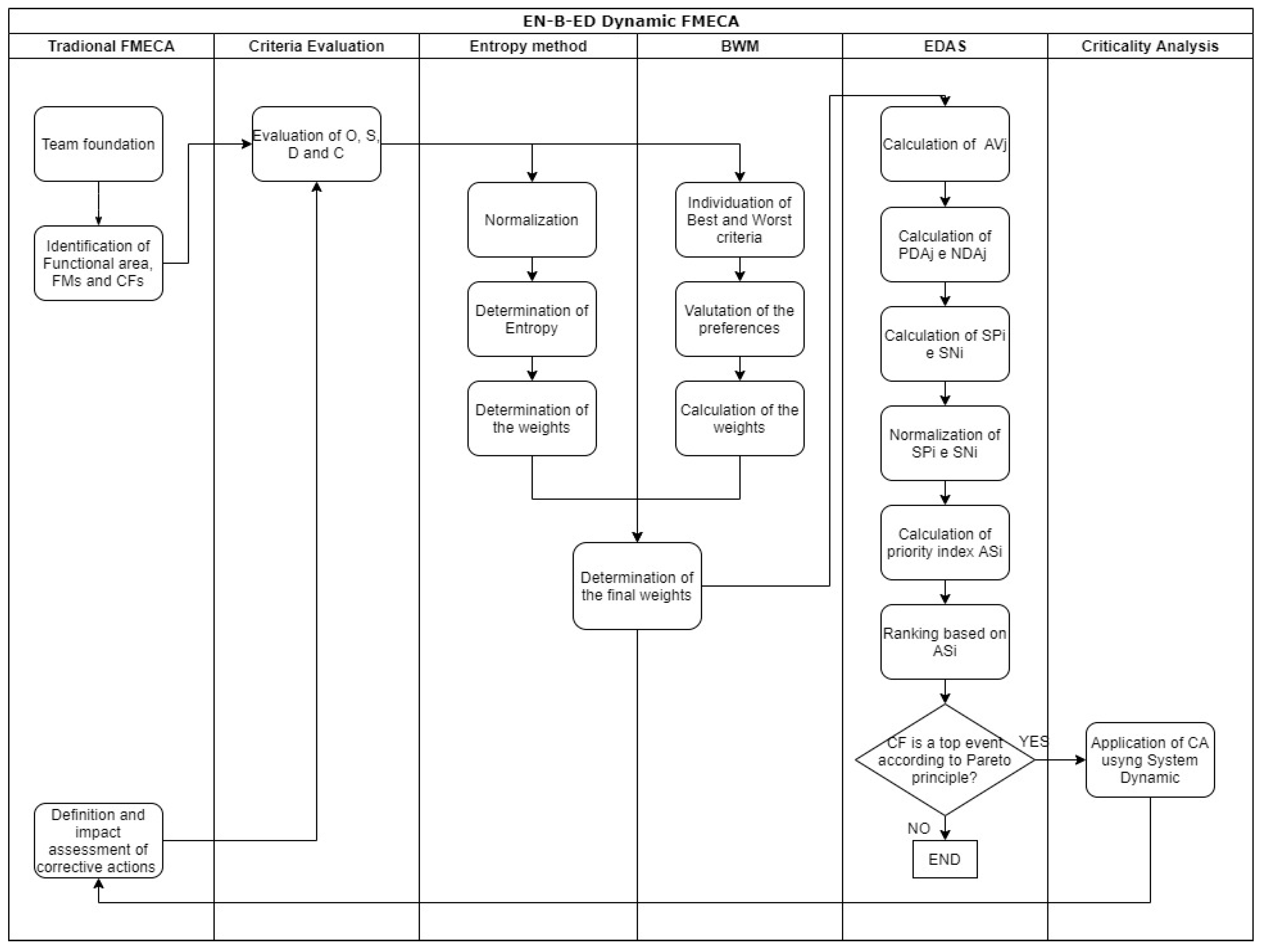
Each step of this proposed method is explained in detail in this section. Figure 1 represents the logical sequence of an operations flowchart to execute the EN-B-ED Dynamic FMECA correctly.

2.1. Multidisciplinary Team Creation, Machine Breakdown into Functional Units and Identification of FMs and CFs

The proposed methodology starts from a classical FMEA analysis with a multidisciplinary team of specialists who identify the critical areas of the system analysing them. The output of this analysis is the identification of the possible failure modes and the related causes and effects. Hence, the criteria that best describe the risk associated with FMs are defined, and the criterion for each possible cause of the fault is evaluated.

2.2. Evaluation of the Factors O, S, D, and C

The first innovation point of EN-B-ED Dynamic FMECA analysis concerns the criteria used. We added the cost, C, in addition to the three traditional FMEA criteria, O, S, and D, to consider the costs arising from the fault occurrence. This term considers:

• Costs of non-production

  $$C_{MP}=\left(C_{hp}\ast N_p\ast T_i\right)+\left(Q_p\ast P_p\ast T_i\right)+\left(C_{hps}\ast N_p\ast T_i\right)$$

  (2)

  where $C_{hp}$ is the hourly cost of the production labour, $N_p$ is the number of workers, $T_i$ is the time of the maintenance intervention to restart the machine, $Q_p$ is the average quantity produced per hour, $P_p$ is the average price of the finished product, $C_{hips}$ is the hourly overtime cost of the production labor. Therefore, the first term takes into account the cost of the production unable to work during downtime, the second term takes into account the hidden costs resulting from the lack of production, and the last term instead takes into account the cost to be incurred if it is decided to pay overtime to recover lost production.
• Labour costs

  $$C_{MDO}=\left(C_{hm}\ast N_m\ast T_i\right)$$

  (3)

  where $C_{hm}$ is the hourly cost of maintenance workers, $N_m$ is the number of maintenance workers, and $T_i$ is the maintenance intervention time.
• Costs of spare parts used

  $$C_R={\displaystyle \sum }_{i=1}^n{C}_i{Q}_i$$

  (4)

  where $C_i$ is the cost of the i-th spare part and $Q_i$ is the number of spare parts used.

  $$C=C_{MP}+C_{MDO}+C_R$$

  (5)

2.3. Criteria’s Weights’ Calculation through Entropy Method and Best Worst Method (BWM)

Once obtained, the starting matrix in which the possible alternatives are on the rows, the criteria are on the columns, and the evaluations constitute the heart of the matrix; moreover, each criterion’s weight must be identified.

In the traditional FMEA, a severe weakness, much discussed over the years, is the lack of different weights for the criteria; one factor may be predominant compared to the others.

This problem has been solved using a combination of the Entropy method and BWM to obtain the weights. A choice was made to not use methods that use language variables because these are difficult to manage and require adept experience to be used most effectively. There is also a risk of incorrectly considering some subjective values, as it is related to individual skills [31].

Although experts’ subjective opinions are intrinsically present in the data structure, the combination with BWM has been made to take more account of business ideas [28]. Moreover, using the two methods makes the method replicable in any company, even where no objective maintenance data is available.

After calculating the weights with the two methods, a simple average or a weighted average of the values can be done; this depends mainly on how much the business ideas influence the maintenance aspects.

The Entropy method, according to [32], will be applied as follows:

• The data of the matrix will be normalised to ensure a homogeneous and direct comparison between the criteria:

  $$Z_{ij}=\frac{x_{ij}}{{{\displaystyle \sum }}_{i=1}^n{x}_{ij}}$$

  (6)
• Entropy is calculated for each criterion:

  $$E_j=\left(-\frac{1}{\ln \left(n\right)}\right)\ast {\displaystyle \sum }_{i=1}^n\left(Z_{ij}\ast \ln z_{ij}\right)$$

  (7)
• The values $d_j$ are calculated:

  $$d_j=1-E_j$$

  (8)
• Finally, weights $W_j$ are calculated:

  $$W_j=\frac{d_j}{{{\displaystyle \sum }}_{j=1}^m{d}_j}$$

  (9)

The greater the weight of criterion j, the more critical the criterion j. If the values of criterion j are almost equal, then it will be assigned a small weight, because the entropy method is an objective method based solely and exclusively on the data structure and is in no way influenced by managerial policies [32].

According to the aforementioned studies, the BWM will be applied as follows:

• The most important criterion and the least important criterion will be identified;
• Preferences of the most important criterion are expressed over the others by giving a number from one to nine, which obtains a line vector;
• Preferences of the least important criterion are expressed by giving a number from one to nine. A column vector is obtained;
• Finally, a problem of optimisation of the type is solved:

  $$\begin{array}{ccc}& \{\min {\xi }_L\P & \\ & & \begin{array}{l}\hspace{1em}subjected to\\ \left|w_B-a_{Bj}{w}_j\right|\le {\xi }_L\\ \left|w_j-a_{jw}{w}_w\right|\le {\xi }_L\\ {\displaystyle \sum _{j=1}^m}{w}_j=1\end{array}\\ w_j\ge 0\}& & \end{array}$$

  (10)

  to obtain the weights of the criteria.

2.4. Calculation of Final Weights

Once $w_{e\left(e\right)}$ and $w_{j\left(BW\right)}$ have been calculated, the final weights must be determined in the following way:

$$w_j=E\ast w_{j\left(e\right)}+BW\ast w_{j\left(BW\right)}$$

(11)

where E is the weight to give to data from maintenance and BW is the weight to give subjective data from experts.

2.5. Application of the EDAS Method to Rank Alternatives

The EDAS method (evaluation based on distance from the mean solution) is a relatively recent MCDM problem-solving technique. It derives from considerations made on two methods, namely TOPSIS and Weighted Sum Method (WSM). It calculates the ${\mathrm{AV}}_{\mathrm{j}}$ (mean value) for each j-th criterion and evaluates each alternative’s distance from this value.

According to Trinkūnienė, Podvezko, and Zavadskas [32] seven steps must be followed:

• Calculate the average solution for each criterion ${\mathrm{AV}}_{\mathrm{j}}$

  $${\mathrm{AV}}_{\mathrm{j}}=\frac{{{\displaystyle \sum }}_{\mathrm{i}=1}^{\mathrm{n}}{\mathrm{x}}_{\mathrm{ij}}}{\mathrm{n}}$$

  (12)
• Calculate the mean positive distance ${\mathrm{PDA}}_{\mathrm{ij}}$ for the benefit and disadvantage criteria:

  ▪

  Benefit

  $${\mathrm{PDA}}_{\mathrm{j}}=\frac{\left(\max \left\{0,{\mathrm{x}}_{\mathrm{ij}}-{\mathrm{AV}}_{\mathrm{j}}\right\}\right)}{{\mathrm{AV}}_{\mathrm{j}}}$$

  (13)

  ▪

  Disadvantage

  $${\mathrm{PDA}}_{\mathrm{j}}=\frac{\left(\max \left\{0,{\mathrm{AV}}_{\mathrm{j}}-{\mathrm{x}}_{\mathrm{ij}}\right\}\right)}{{\mathrm{AV}}_{\mathrm{j}}}$$

  (14)

• Calculate the mean negative distance ${\mathrm{NDA}}_{\mathrm{ij}}$ for the benefit and disadvantage criteria:

  ▪

  Benefit

  $${\mathrm{NDA}}_{\mathrm{j}}=\frac{\left(\max \left\{0,{\mathrm{AV}}_{\mathrm{j}}-{\mathrm{x}}_{\mathrm{ij}}\right\}\right)}{{\mathrm{AV}}_{\mathrm{j}}}$$

  (15)

  ▪

  Disadvantage

  $${\mathrm{NDA}}_{\mathrm{j}}=\frac{\left(\max \left\{0,{\mathrm{x}}_{\mathrm{ij}}-{\mathrm{AV}}_{\mathrm{j}}\right\}\right)}{{\mathrm{AV}}_{\mathrm{j}}}$$

  (16)

• Using the weights of the previously calculated criteria, the weighted sums are calculated, ${\mathrm{SP}}_{\mathrm{i}}$

  $${\mathrm{SP}}_{\mathrm{i}}={\displaystyle \sum }_{\mathrm{j}=1}^{\mathrm{m}}{\mathrm{w}}_{\mathrm{j}}\times {\mathrm{PDA}}_{\mathrm{j}}$$

  (17)
• Using the weights of the previously calculated criteria, the weighted sums are calculated, ${\mathrm{SN}}_{\mathrm{i}}$

  $${\mathrm{SN}}_{\mathrm{i}}={\displaystyle \sum }_{\mathrm{j}=1}^{\mathrm{m}}{\mathrm{w}}_{\mathrm{j}}\times {\mathrm{NDA}}_{\mathrm{j}}$$

  (18)
• The weighted sums are normalised

  $${\mathrm{NSP}}_{\mathrm{i}}=\frac{{\mathrm{SP}}_{\mathrm{i}}}{\max \left\{{\mathrm{SP}}_{\mathrm{i}}\right\}}$$

  (19)

  $${\mathrm{NSN}}_{\mathrm{i}}=1-\frac{{\mathrm{SN}}_{\mathrm{i}}}{\max \left\{{\mathrm{SN}}_{\mathrm{i}}\right\}}$$

  (20)
• The priority index, ${\mathrm{AS}}_{\mathrm{i}}$, is calculated

  $${\mathrm{AS}}_{\mathrm{i}}=\frac{1}{2}\left({\mathrm{NSP}}_{\mathrm{i}}+{\mathrm{NSN}}_{\mathrm{i}}\right)$$

  (21)

The ranking of the possible causes of failure is evaluated following the descending order of the AS index.

2.6. Criticality Analysis (CA)

The CA consists of a qualitative, quantitative, or semi-quantitative analysis used to identify the critical causes of a system failure or those where it is convenient to intervene most urgently. There are several methods to perform this analysis. One of these is to use the Hazard Score Matrix, in which only S and O are considered to assess the various risks of hazards (and incidents), and whose product is compared either with threshold values or through the Pareto principle analysis [33]. according to which 20% of the causes of faults cause 80% of the total faults.

The Pareto principle of 80–20 is applied to the EDAS method’s ranking to identify the most important critical issues.

In traditional FMECA, once the causes of critical failures have been identified, they are analysed individually and in a static way, i.e., without seeing how they evolve. Furthermore, in doing so, the interdependencies between the different failure modes are not considered [12,31]. This is a weakness strongly discussed by scholars—the lack of dynamism. In doing so, one never looks at the machine’s totality and how its conditions change over time.

A criticality analysis with a System Dynamics model is carried out to overcome this problem.

System Dynamics is an approach to considering a system not as a set of single independent components but as a single complex system in which causal relationships feed over time. Usually, simulation software captures the system’s relational aspects and studies its behaviour over time. The concept of time is essential because, in classic FMECA, the causes of failure are considered one at a time, without considering how one influences the other and how the sum of their contributions accumulates over time, increasing the system’s criticality.

In order to use System Dynamics correctly, it is first necessary to understand and be able to adequately represent the system’s behaviour, finding and highlighting how the elements are reciprocally connected.

Then, the criticality analysis is conducted in a dynamic way to examine how the simultaneity of the various causes of failure and their interactions influence the total probability of failure.

2.7. Definition and Impact Assessment of Corrective Actions

Once the system’s criticalities have been identified, technicians and experts must be brought together to identify the corrective actions to be taken to lower the risk associated with the system. In this case, thanks to the use of System Dynamics, the technicians do not look only at the critical component, but also at the totality of the system, questioning the influence that the various components have on each other and thus identifying corrective actions capable of lowering the entire failure risk associated with the machine.

Once corrective actions are identified, they are implemented and evaluated. To do this, the cycle illustrated in Figure 1 is repeated.

This generates an infinite cycle aimed at continuously improving the system’s efficiency.

3. Case Study

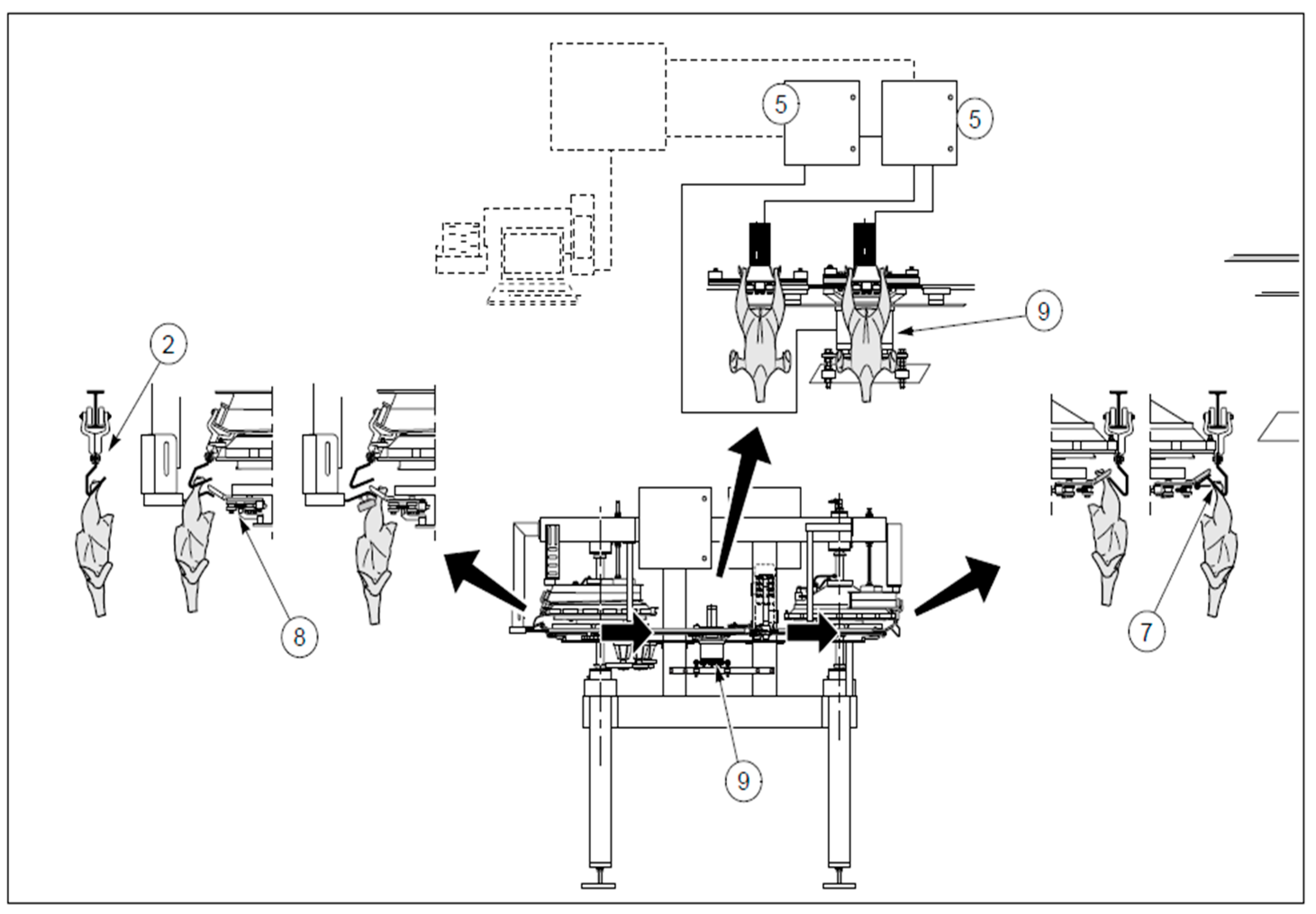
Our case study focuses on assessing a machine called TR-CS recoupling in a manufacturing company in the agri-food sector. Figure 2 shows a top view of this.

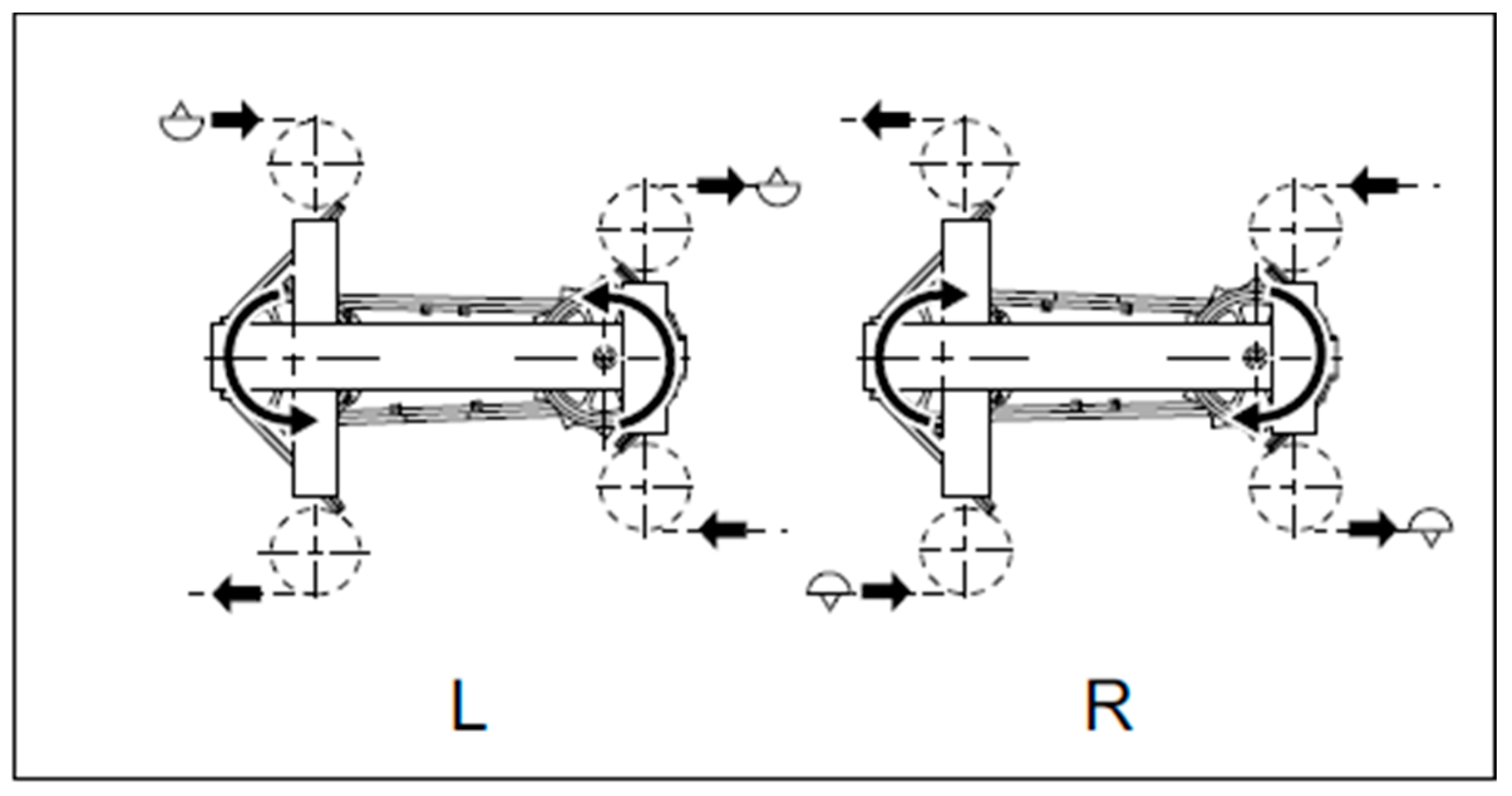
This machine allows the transfer from one chain to another automatically. In Figure 3, the TR-CS coupling operation is shown.

The chickens arrive from the cooling tunnel, where they remain for at least 3 h, hanging from the hook (in Figure 3 indicated with the number 2) of the cooling chain. The chicken is attached to the hook of the tunnel chain when it is still wet and then stops in the cooling tunnel, where the temperature is lowered to better process the meat and allow it to dry. The chicken is welded more firmly to the hook, which is aligned with the front of the trolley of the transfer station (in Figure 3, indicated with the number 8) as it dries, making it more difficult to detach. If the hook is not aligned, the movement of the machine can damage or even break the chicken shanks. The transfer is enabled from the hook to the trolley by an extraordinary guided positioned to place the chicken. When the trolley exits the drive disc, it accelerates as the distance between the products increases, and it is driven to the weighing unit by a toothed belt (in Figure 3, indicated with number 9). The product is weighed, and the relative data are provided to the control system during carriage on the side of the calibration line (in Figure 3, indicated with number 5). The process is mirrored to the one just described on the right side, the side of the calibration line. The trolley is then aligned with the hook of the calibration chain (indicated by the number 7 in Figure 3) and a suitably positioned guide allows the chicken to be hooked to the calibration chain. Here, the work of the guide is less onerous than that of the release guide because the chicken does not have time to “weld” to the carriage, and therefore it is easier to detach it. The process is equipped with a series of sensors that identify the hook “0” of the chains, which allow the machine to detect the presence of chickens, count them, weigh them, and match all the product data.

3.1. Multidisciplinary Team Creation, Machine Breakdown into Functional Units, Identification of FMs and CFs

The first step of our analysis is to form an interdisciplinary team. It is essential to bring together people with different technical backgrounds and several years of experience to identify all possible ways of system failure.

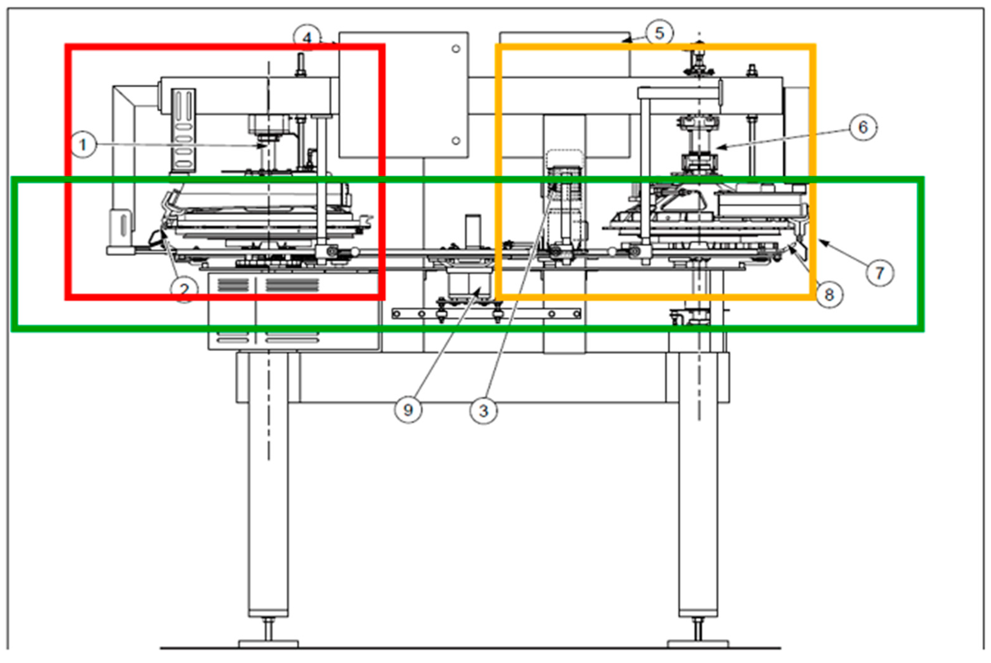
The team, during a couple of meetings, also thanks to the help of the machine manuals, has broken down the machine into six functional units:

• Tunnel chain;
• Release chicken station (In Figure 4 indicated with a red box);
• Transfer station (In Figure 4 indicated with a green box);
• Hooking chickens’ station (In Figure 4 indicated with an orange box);
• Calibration chain;
• Electric circuit.

Once the system was broken down into the various functional units, the functional units’ main components were then identified. The possible failure modes have been identified for each component and the effects and causes of failure for each failure mode. The machinery data used are collected in the supplementary file.

3.2. Evaluation of the Factors O, S, D, and C

After this first work of breaking down the machinery and identifying faults and causes, the team focused on evaluating the four factors O, S, D, and C. They followed their experience and a series of data from the maintenance management software.

In Table S1—FMECA table (Supplementary Materials), there is the starting matrix of the case study.

3.3. Criteria’s Weights Calculation through Entropy Method and Best Worst Method (BWM)

The next step of the proposed method involves applying the Entropy method to calculate the criteria’ weights. You can refer to Table S2—ENTROPY (Supplementary Materials) for a complete analysis. Once the criteria weights have been calculated with the Entropy method, one can calculate the weights with the BWM.

3.4. Calculation of Final Weights

Having the weights of the two criteria, all that remains is choosing their relative importance to proceed with the final calculation of the weights.

In our case, according to the opinion of the team, the same weight to the two methods was assigned:

$$w_j=0.5\ast w_{j\left(E\right)}+0.5\ast w_{j\left(BWM\right)}$$

(22)

Therefore, in our case study, the two methods have the same importance, therefore both the subjective data expressed a priori by the experts and the objective maintenance data were considered equally important.

Once the definitive weights of the criteria have been calculated, one can move on to the application phase of the EDAS method to calculate the ranking of the alternatives.

3.5. Application of the EDAS Method to Rank Alternatives

Before reaching the criticality analysis, the last step of our methodology involves the use of the EDAS method to calculate the ranking of alternatives.

Microsoft Excel was used to apply the EDAS method, resulting in a worksheet full of information. For simplicity of representation, an extract of the fundamental part relating to the calculation of the Appraisal score and ranking are reported in the Supplementary Materials (Table S4—EDAS (Supplementary Materials)).

3.6. Criticality Analysis (CA)

Our case study carried out the criticality analysis using Vensim PLE x64, a widely used software in System Dynamics models’ simulation.

Before moving on to the construction of a CLD and then to the simulation, it is necessary to identify the critical events using the Pareto principle. This famous principle has often been used in criticality analysis [34].

The critical events found with the analysis carried out are those that the experts indicated a priori as critical events in the machine operation’s deployment. Furthermore, in this study, the model proposed leads to actual results.

For ease of representation and analysis, it has been decided to exclude the causes CF55/CF57/CF58/CF70/CF71/CF72/CF73/CF80 from the analysis. The choice was taken into consideration since the causes are the same. Furthermore, all the actions and analyses that were carried out on the causes related to the tunnel chain and the chicken release station can be proposed again strictly for the causes CF55/CF57/CF58/CF70/CF71/CF72/CF72/CF73/CF80 related to the calibration chain and the chicken release station.

Besides, the causes related to the chicken release station and the calibration chain are the most serious for the reasons mentioned above:

• The tunnel chain is considerably longer than the sizing chain; if it breaks, it causes more damage at the economic level;
• The release guide, on the other hand, unlike the hooking guide, is subject to more significant stress and, therefore, more prone to failure.

As already mentioned in this work, a dynamic simulation program is used to simultaneously study the causes of failure and not take them individually as in the traditional FMEA [34].

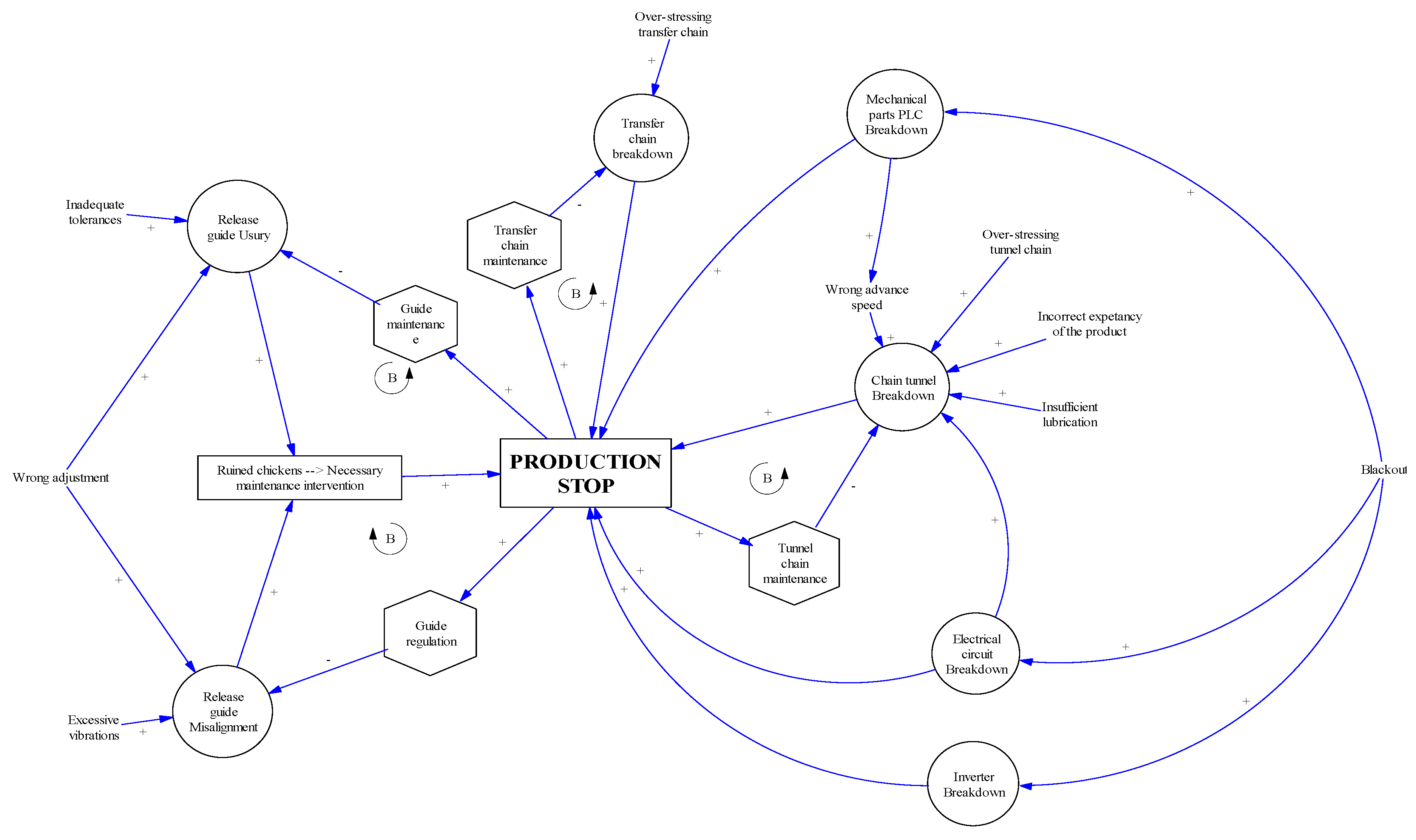
The first step is to represent the causal relationships between the variables present graphically. This diagram is called the Causal Loop Diagram (CLD). Thanks to CLD, it is possible to identify possible strengthening or balancing cycles [35].

These cycles are significant as they tell us if two or more failures increase each other over time or eliminate each other.

In Figure 5, an illustration of our Causal Loop Diagram is presented. To better understand the proposed CLD, a list is provided that explains the representation:

• The causes of failure have been entered without a box;
• The failure modes have been entered in the circles;
• Effects have been placed in rectangles;
• Maintenance actions have been placed in hexes.

In the diagram, thanks to the presence of these maintenance interventions, four balancing loops can be seen:

• FM10-E10-STOP PRODUCTION-Guide Maintenance-FM10;
• FM9-E10-STOP PRODUCTION-Guide Regulation-FM9;
• FM1-STOP PRODUCTION-Tunnel chain maintenance-FM1;
• FM26-STOP PRODUCTION-Transfer chain maintenance-FM26.

Since each cause has its stochastic properties, the probability distribution that best suits the different causes of failure must be identified:

• Due to the causes CF11/CF86/CF91 (Blackout), CF2 (Incorrect feed speed), CF3 (Incorrect product life forecast), and CF20 (Inadequate tolerances) being purely random events, the model that best interprets the behaviour is the exponential one;

  $$F\left(t\right)=1-ex{p}^{-\lambda \ast t}$$

  (23)

  $$\mathrm{f}\left(\mathrm{t}\right)=\lambda \ast ex{p}^{-\lambda \ast t}$$

  (24)

  $$\mathrm{h}\left(\mathrm{t}\right)=\frac{f\left(t\right)}{1-F\left(t\right)}=\lambda$$

  (25)

  where λ is the event occurrence frequency.
• For the causes CF18/CF21 (Wrong adjustment), CF19 (Excessive vibrations), CF38 (Over-stressing), CF1 (Insufficient lubrication), and CF4 (Over-stressing), being causes of failure of mechanical components, the model that best represents their behavior is Weibull’s model:

  $$\mathrm{F}\left(\mathrm{t}\right)=1-ex{p}^{-{\left(\frac{t}{\alpha }\right)}^{\beta }}$$

  (26)

  $$\mathrm{f}\left(\mathrm{t}\right)=\frac{\beta }{{\alpha }^{\beta }}\ast t^{\beta -1}\ast ex{p}^{-{\left(\frac{t}{\alpha }\right)}^{\beta }}$$

  (27)

  $$\mathrm{h}\left(\mathrm{t}\right)=\frac{f\left(t\right)}{1-F\left(t\right)}= \frac{\beta }{{\alpha }^{\beta }}\ast t^{\beta -1}$$

  (28)

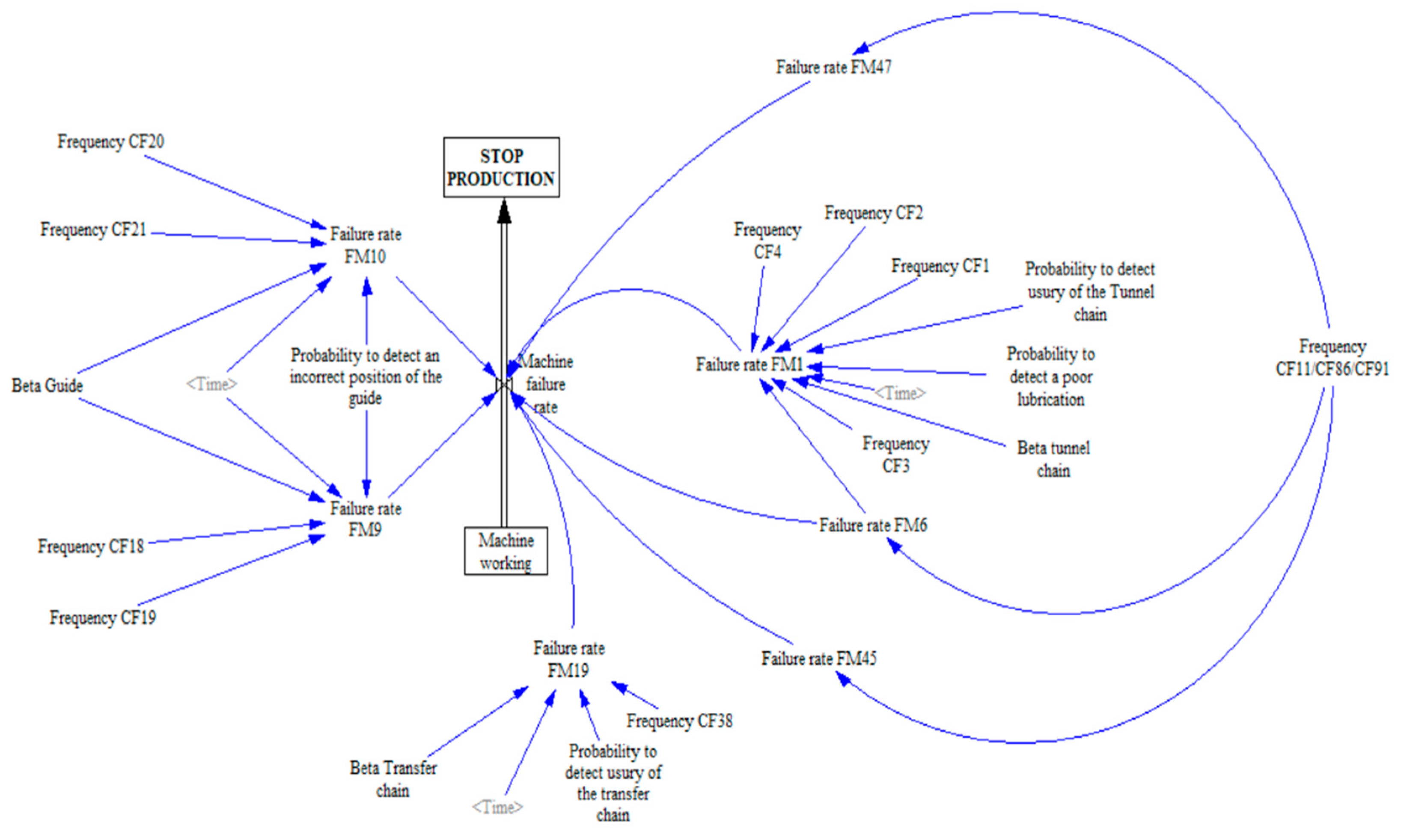
The model under analysis with the relationships is shown in Figure 6.

As shown in Figure 6, no maintenance variables have been inserted in the model, not because the maintenance activities have not been considered, but because they have been incorporated within the failure rate functions of the various failure modes.

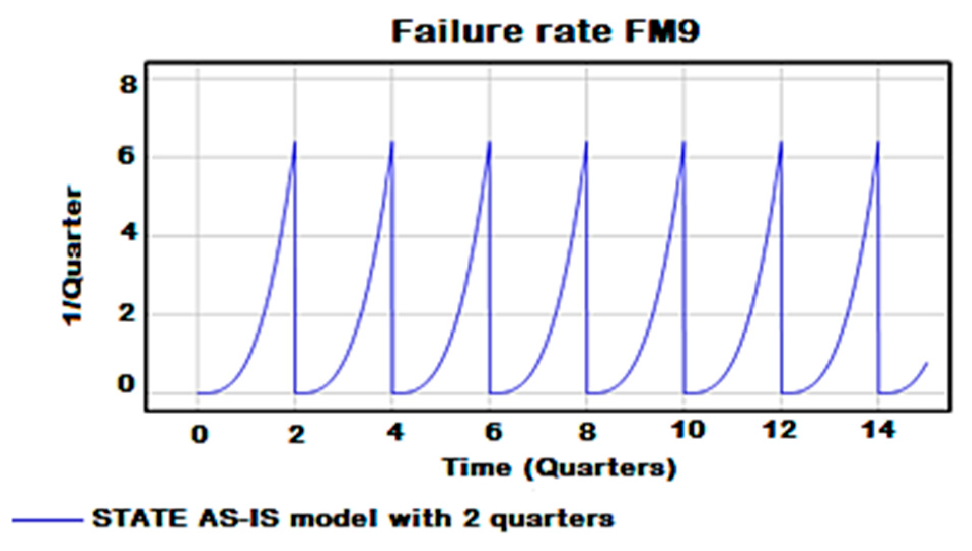
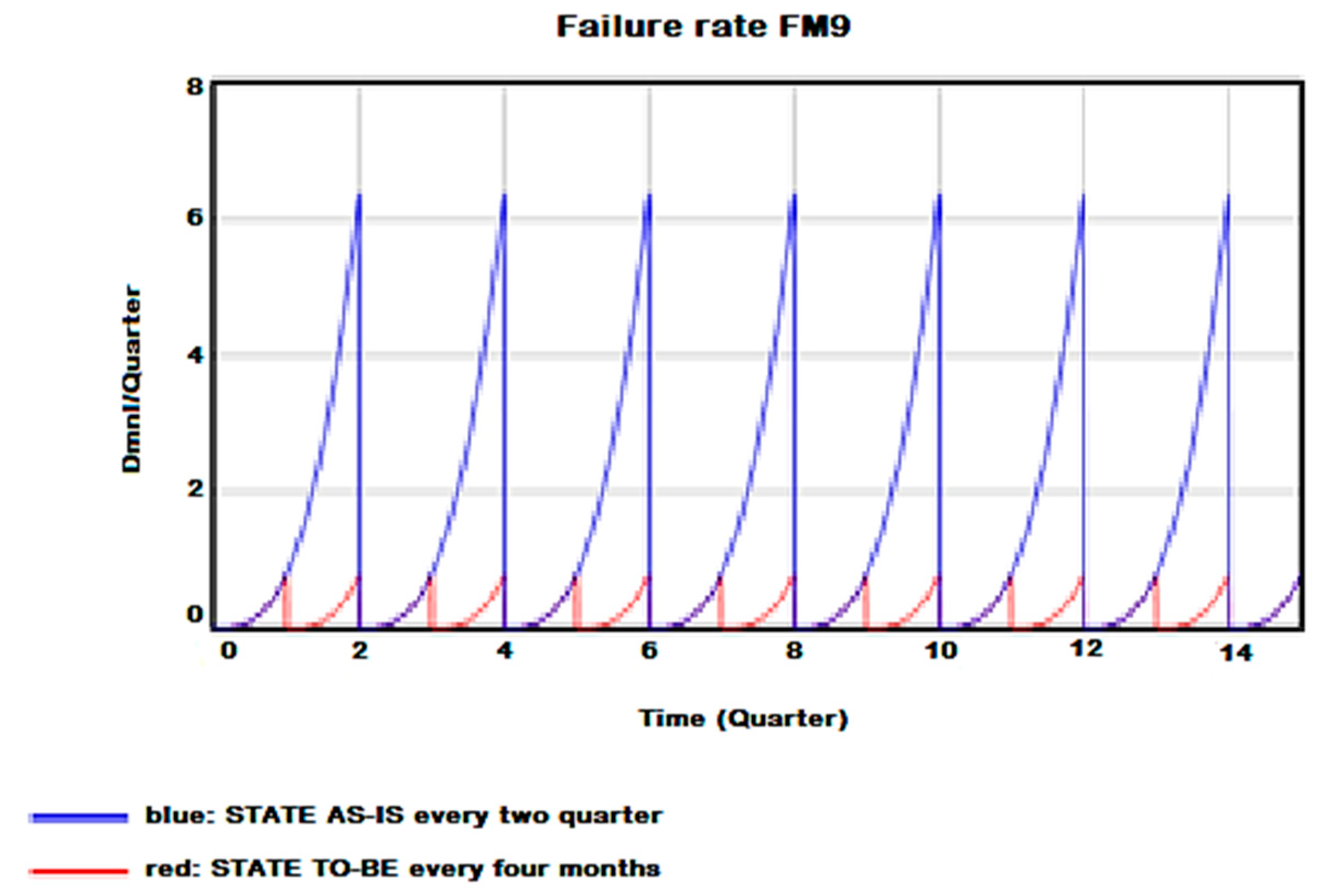
For the FM9 failure mode, a misalignment of the guide of an IF THEN ELSE cycle, with a cycle time of two quarters, has been set. This means that, thanks to the adjustment operations carried out every two months, the conditions of the guide, seen from the point of view of the alignment, are returned to the 0 state, as shown in Figure 7.

On the other hand, for the failure mode FM10 shown in Figure 8, a cycle time of 2 years was set. This is because the guide is changed every two years, therefore its wear conditions are reset.

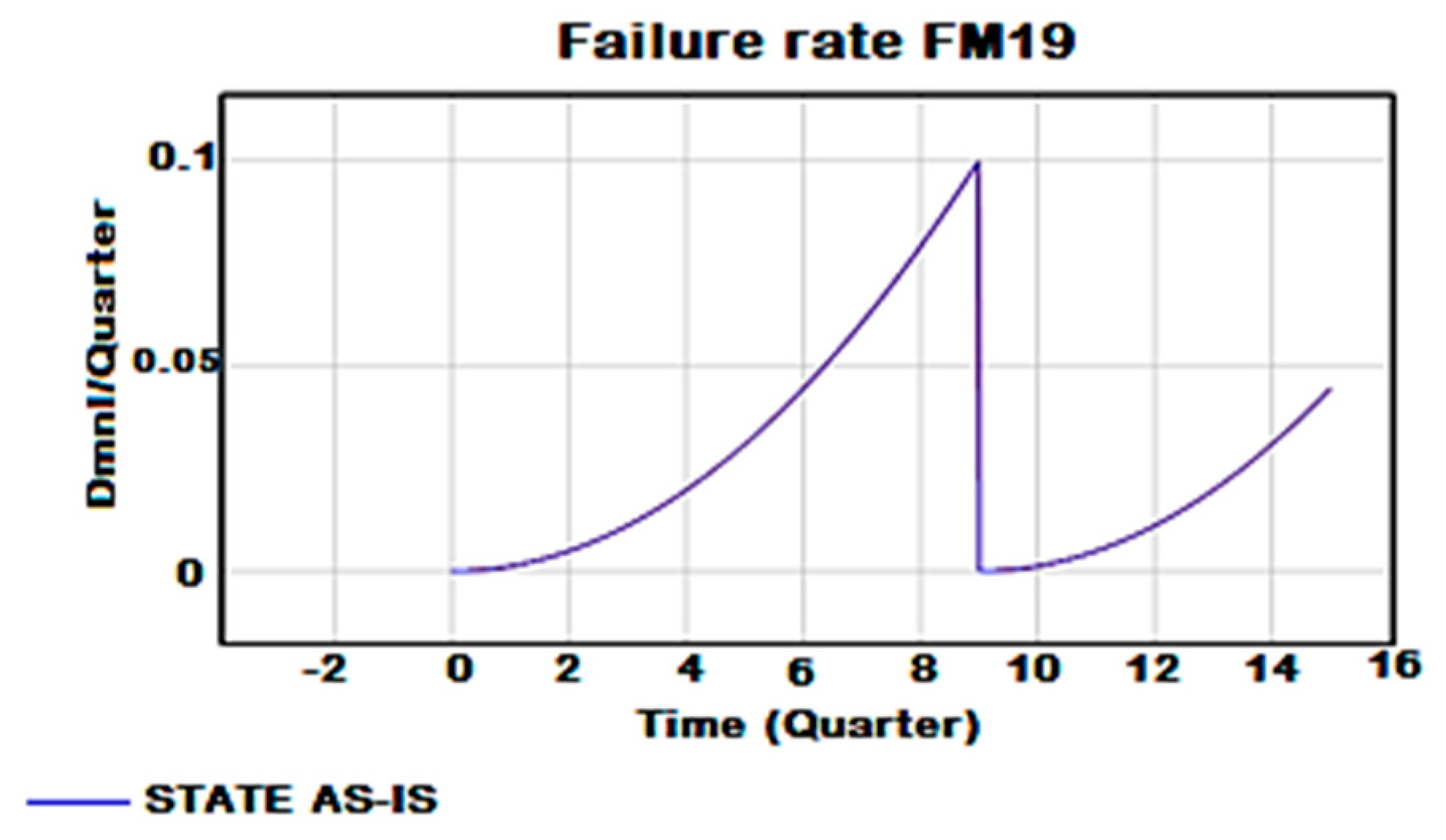
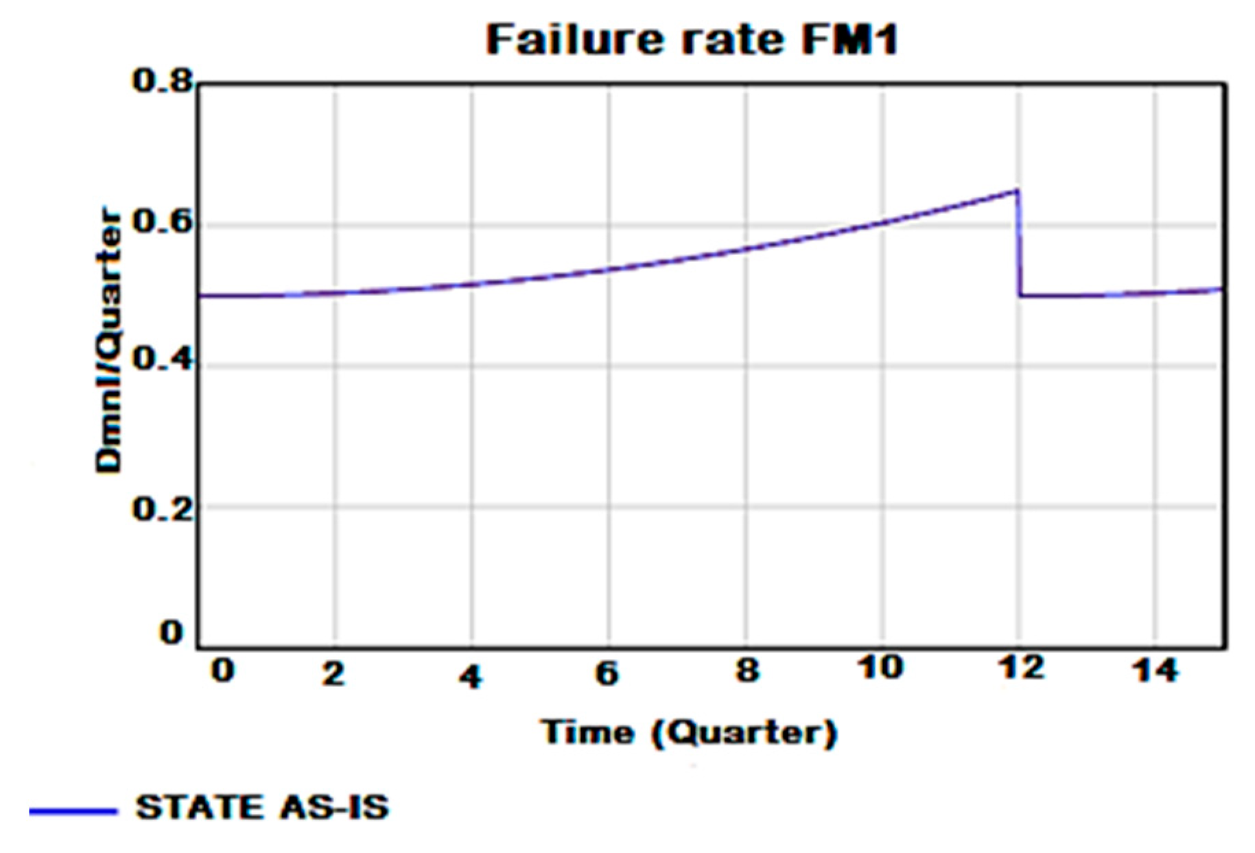
For the failure modes FM19 (transfer chain breakage) (Figure 9) and FM1 (tunnel chain breakage) (Figure 10), on the other hand, cycle times have been set as 3 and 4 years, respectively, because the two chains are changed with such intervals as required by the preventive maintenance plan drawn up by the manufacturer.

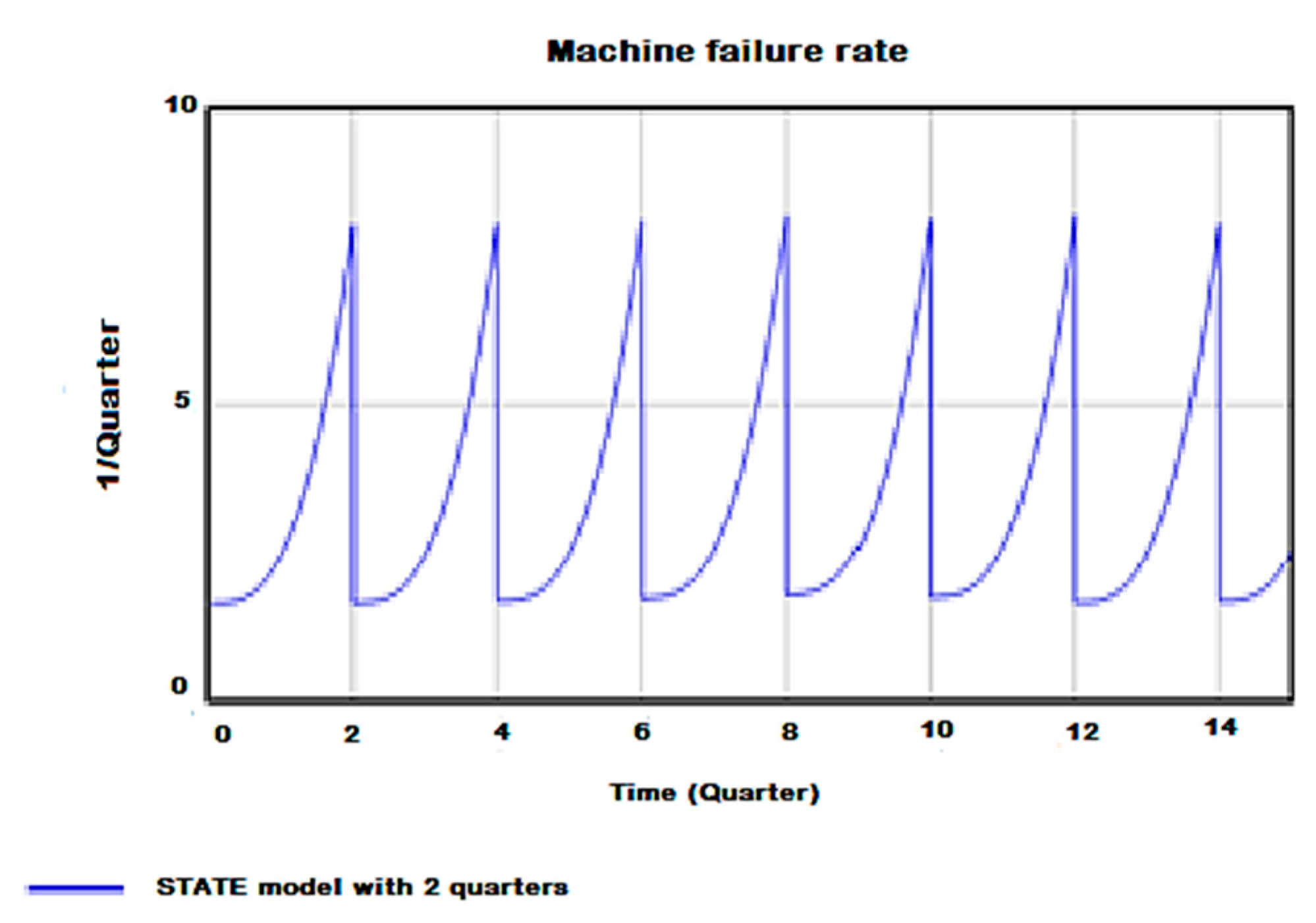
Once the trends of the various failure rates have been identified, all that remains is to identify that of the machine.

To do this, the total failure rate is obtained from the probability that all events can occur. The events can be considered as s-independent. The complete system status is presented in Figure 11.

From the graph (Figure 11), it can be seen how the maintenance actions greatly influence the system’s failure rate.

Looking at all the graphs, you can also guess that the failure machine rate, the failure rate of the entire machine, is greatly influenced by the failure rate of the FM9 guide misalignment. This is because it is the most frequent failure that occurs.

The simulation was made regarding the AS-IS status of the system, thus considering the maintenance policies adopted in the company.

In the following, some corrective actions and their possible results are presented.

3.7. Definition and Impact Assessment of Corrective Actions

As seen, our machine’s critical events concern the tunnel chain, the transfer chain, and the release guide.

Through simulation, it was identified that the component that has the greatest impact on the trend of the machine failure rate is the chicken release guide.

This component performs a fundamental task and must always be aligned in the right position. Unlike the chicken hooking guide which plays a similar role, its task is made more complicated by the fact that the chickens arrive from the cooling tunnel where they have stayed for at least 3 h. This period causes the chicken to fasten to the hook of the tunnel chain, arriving at the chicken release area, and the guide must undergo strong stress to be able to detach the chicken from the hook and must always be aligned correctly; otherwise, it runs the risk of spoiling or dropping the chicken (Figure 12).

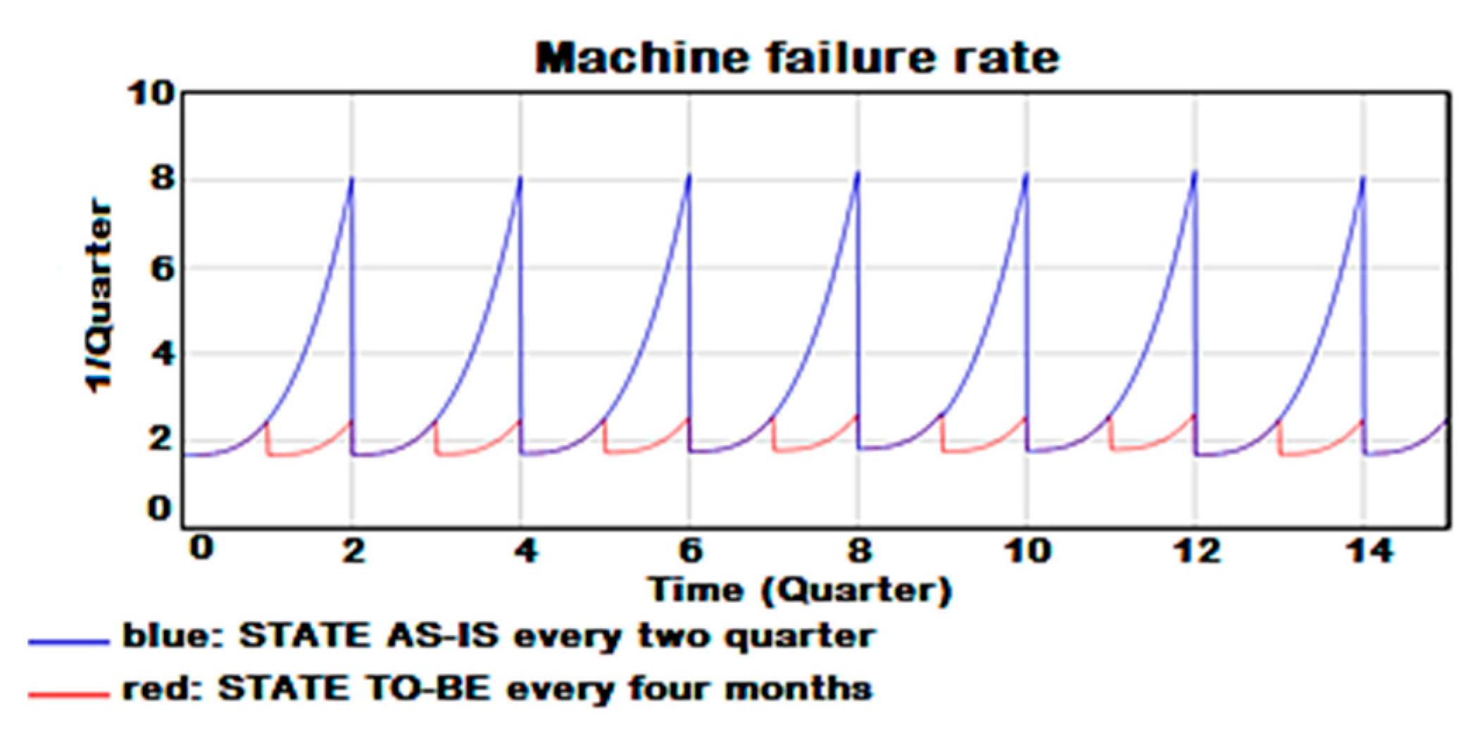
To avoid fewer failures and lower the chicken guide failure rate (

Table 3. FM9 Failure rate.

Time (Quarter)	0	0.5	1	1.5	2	2.5	3	3.5	4
Failure rate FM9: STATUS TO-BE every four months	0	0.1	0.8	0.1	0.8	0.1	0.8	0.1	0.8
Failure rate FM9: STATUS AS-IS every two quarters	0	0.1	0.8	2.7	6.4	0.1	0.8	2.7	6.4

), one might consider increasing the guide adjustment frequency. This first action allows us to lower the probability of the failure occurring drastically.

Therefore, an 87.5% improvement in the guide failure rate is obtained with this first corrective action.

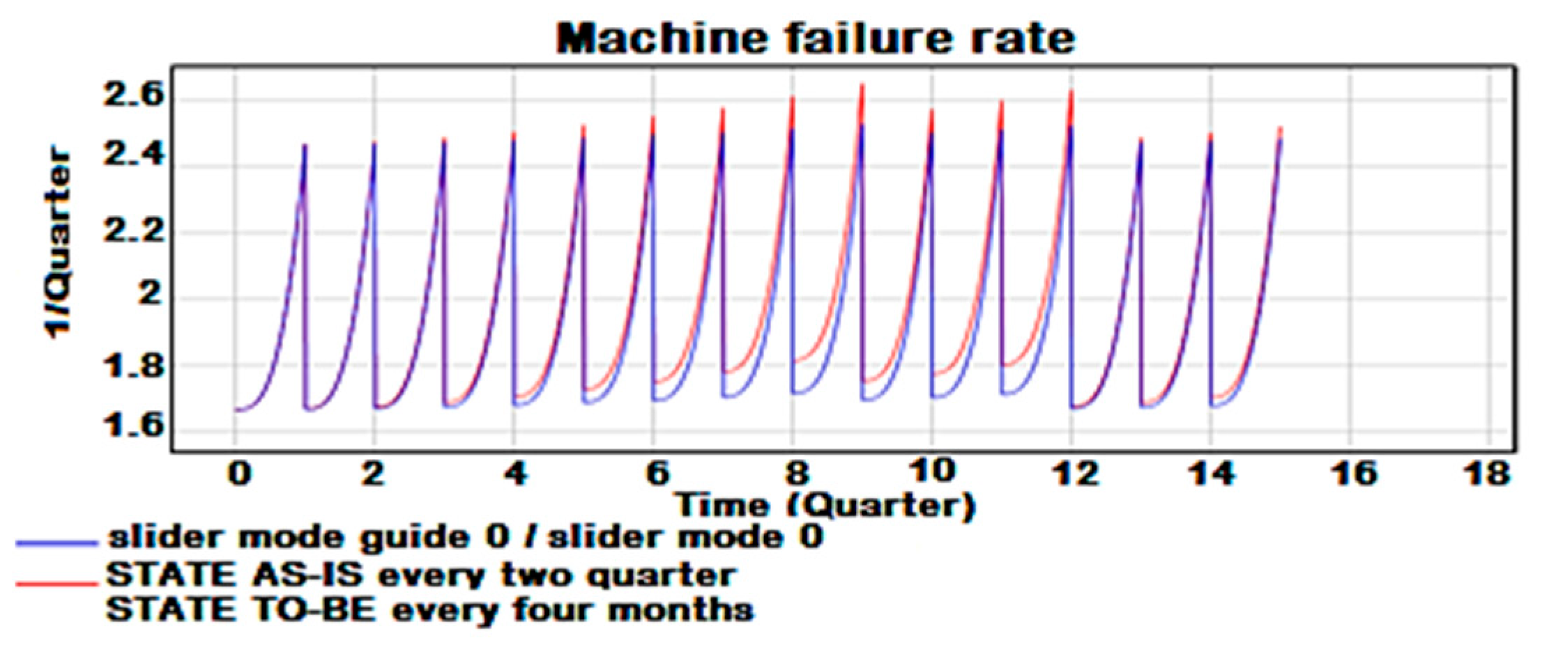
Therefore, to see how the situation changes in the case of the failure rate of the entire system, a significant improvement is also noted here, as can be seen in

Table 4. AS-IS machine failure rate comparison.

Time (Quarter)	STATE TO-BE Every Four Months	STATE AS-IS Every 2 Quarters
0	1.7	1.67
1	2.47	2.47
2	2.48	8.08
3	2.49	2.49
4	2.50	8.10
5	2.53	2.53
6	2.55	8.15
7	2.58	2.58
8	0.26	0.82
9	2.65	2.65
10	0.26	0.82
11	2.60	2.60
12	2.63	8.23
13	2.49	2.49
14	0.25	0.81
15	2.52	2.52

and Figure 13 from a maximum of 8.23 to a maximum of 2.65, with an improvement of 67.8%

Other actions that can be implemented to lower the entire system’s failure rate are to try to increase the detectability of some failure modes before they occur. In particular, two scenarios can be evaluated to reduce the failure rate of the chains:

The first scenario concerns the breakage of the electrical parts due to the blackout. Obviously, nothing can be done about it because it depends on external causes. The only actions that could be implemented to eliminate those failure modes are to install some emergency generators. However, this is a very expensive action that is not worth the risk due to the very low frequency of blackouts.

The second scenario analyses the failure rate of the chains due to their wear. It could be established either by a greater number of checks by the maintenance technicians to identify signs of wear of the chains or establish automatic checks with sensors capable of identifying chain length variations.

The hypothesis is that it is possible to detect the fault of 90% of failures, thanks to one of these two choices.

Figure 14 and Table 4 show how the situation changes can be seen.

There is a minimum improvement of about 5% from the frequency of the chains’ breakings which is already minimal.

Indeed, it is advisable to increase the inspections by the maintenance technicians to intervene promptly at every slightest deviation of the chain from the initial conditions to avoid accelerated wear. However, installing automatic detection systems such as sensors is not advisable because they are still expensive systems.

The first safe step on which to intervene is the chicken release guide.

A few corrective actions achieve great results in machine operation, thus limiting production stops to a minimum.

4. Conclusions

Companies’ risk management is increasingly fundamental in manufacturing companies with an almost saturated production cycle.

It is fundamental to prevent the occurrence of a failure as much as possible because it leads, in most cases, to a loss of production and, therefore, to severe economic losses.

In the presented work, a development of the traditional FMEA is proposed, wherein some innovative aspects have been added to eliminate some deficiencies present in the traditional FMEA/FMECA.

This new methodology combines the Entropy and BWM methodology with the EDAS and System Dynamics, FMECA. All this was implemented in a case study of an important Italian company in the agri-food sector, and the use of simulation allowed us to consider the dynamic aspects and the relationships between the various failures, which is impossible to do in a standard FMEA analysis in which the causes are analysed individually and statically show a reliable performance.

Therefore, the analysis conducted shows how it can be possible to reduce the machine failure rate. In this regard, a sensitivity analysis has been carried out to support the work carried out. Despite this new combined approach proposed, this study focuses on traditional machinery that does not consider the new technological aspects of Industry 4.0. We are implementing a new research that will not ignore the presence of sensors and Industry 4.0 on the machinery. In conclusion, the new research route will include the use of the application of Machine Learning to prevent faults and minimise the down time of the machine.