Structural Characteristics of Ion Holes in Plasma

Abstract

Ion holes refer to the phase-space structures where the trapped ion density is lower at the center than at the rim. These structures are commonly observed in collisionless plasmas, such as the Earth’s magnetosphere. This paper investigates the role of multiple parameters in the generation and structure of ion holes. We find that the ion-to-electron temperature ratio and the background plasma distribution function of the species play a pivotal role in determining the physical plausibility of ion holes. It is found that the range of width and amplitude that defines the existence of ion holes splits into two separate domains as the ion temperature exceeds that of the electrons. Additionally, the present study reveals that the ion holes formed in a plasma with ion temperature higher than that of the electrons have a hump at its center.

1. Introduction

Solitary wave structures are commonly observed in space, astrophysical and laboratory plasmas [1,2,3,4,5,6,7,8,9]. From the kinetic perspective, these structures are characterized as Bernstein Greene Kruskal (BGK) modes [8,10]. Charged particles will get trapped inside such structures depending on the polarity of wave electrostatic potential and the corresponding sign of charged particles [11]. These solitary wave structures are referred to as ion or electron BGK mode depending on the type of trapped particle species. As the phase-space equilibrium for these modes is characterized by a vortex-type structure, they are also called the ion or electron holes. The ion holes (IHs) are associated with the negative monopolar potential [12], whereas the electron holes (EHs) are associated with the positive monopolar wave potential [13,14]. In-situ observations in the Earth’s magnetospheric regions of bipolar coherent electric field with negative mono-polar potential are indications that IHs are present in such a vicinity [3,7,15]. The Viking satellite [15] first observed the signatures of IHs, followed by the later more frequent detection by FAST satellite [3].

Schamel developed the theoretical models to study the IHs [16,17,18]. Unlike the classical approach, the authors assigned a vortex type distribution to the trapped particles. The integration of both trapped and passing distribution functions in velocity space yields the total charge density as a function of electrostatic potential. The potential is further calculated self-consistently from the Poisson equation. Schamel’s theory places a rather stringent condition on the ion-to-electron temperature ratio for the generation of ion holes [19], but this approach is not well suited to model the observations as the satellite data are not always consistent with such a theoretical prediction. It thus appears that the classical BGK approach is more suitable as it is free from the restriction on the said temperature ratio. Chen et al. [20] thus developed a theory for BGK equilibrium that encompasses both ion and electron holes, which is more general than the approach taken by Schamel. However, certain assumptions implicit in their theory is ambiguous and thus, their solution is not completely general. Recently, Wang et al. [7] reported observations from the Magnetospheric Multiscale (MMS) Mission, which revealed the presence of IHs in Earth’s bow shock region that do not satisfy the temperature ratio condition implied in Schamel’s theory. Aravindakshan et al. [12] improved the theory by Chen et al. [20] and demonstrated that the MMS observations can unambiguously be explained.

The present paper builds upon the work by Chen et al. [20], and further explores the property of IHs under different plasma conditions. The present theoretical formalism assumes that both ions and electrons follow the suprathermal (kappa) distribution function. In general, it is believed that the origin of suprathermal distribution lies in the acceleration by waves in plasma [21,22,23,24,25]. However, on a more specific note, several mechanisms cause the particles to follow suprathermal distribution. Some examples are the superposition of stochastic processes [26], the influence of pickup ions [27], due to quasi-thermal noise [28], the particle acceleration due to shock waves [29] and the variation of the polytropic index in the solar wind protons [30]. Thus these suprathermal distributions of charged particles, often modeled by the kappa distribution, are directly or indirectly observed in diverse regions in space and astrophysical plasmas. Voyager, Cassini, and other interplanetary mission satellite observations report the presence of suprathermal electrons and thermal ions in their respective magnetospheres [31] (and references therein). Observations from the magnetotail of Uranus reported by Voyager reveal the presence of suprathermal ions and thermal electrons with large ion beams directed outward [32,33]. Close to the Earth, Espinoza et al. [34] analyzed the ion kappa parameter distribution in the Earth’s bowshock and plasmasheet. On the other hand, in the heliosheath, magnetosphere of Saturn, and terminal shocks the ions and electrons are found to be in thermal equilibrium [35,36]. By employing the kappa distribution, we may characterize the IHs formed in such diverse regions by choosing different value for the suprathermal kappa parameter.

This paper is organized as follows: In Section 2, we discuss the formulation of BGK IHs, where both ions and electrons follow the suprathermal distribution. Characteristics of IHs and their properties are discussed in Section 3, and the present study is summarized and concluded in Section 4.

2. Theoretical Formalism

We briefly overview the model proposed by Aravindakshan et al. [12] for ion holes in suprathermal plasma. We consider a one-dimensional unmagnetized collisionless plasma system consisting of electrons and ions (protons), commonly found in the Earth’s magnetosphere, other astrophysical and inter-planetary regions. We begin the discourse based upon a one-dimensional Vlasov-Poisson system of equations that governs the dynamics of ion distribution function $f_i$ in collisionless unmagnetized plasma, and adiabatic electrons,

$$\left(\frac{\partial }{\partial t}+V_i\frac{\partial }{\partial x}-\frac{q_i}{m_i}\frac{\partial \Phi }{\partial x}\frac{\partial }{\partial V_i}\right)f_i=0$$

(1)

$$\frac{d^2\Phi }{d{x}^2}=-\frac{q_e{N}_e+q_i{N}_i}{{ϵ}_0}$$

(2)

where $f_i$, $q_i$, $V_i$ and $m_i$ denote the distribution function, charge, velocity, and mass of ions i, respectively. Here $q_e=-e$ for electrons and $q_i=+e$ for ions. $N_e$ and $N_i$ are electron and ion densities such that $N_e=N_i=N_0$. $\Phi$ is the electrostatic potential and ${ϵ}_0$ is the vacuum permittivity. It is convenient to work in a coordinate system in which the ion hole is at rest so that all quantities are time-independent. In such a case, the Equations (1) and (2) reduce to the following normalized form:

$$v\frac{\partial f_i(v,x)}{\partial x}+\frac{1}{2}\frac{\partial \varphi }{\partial x}\frac{\partial f_i(v,x)}{\partial v}=0$$

(3)

$$\frac{d^2\varphi }{d{x}^2}=n_e-n_i$$

(4)

In Equation (4), we have made use of the definition, $n_i={\int }_{-\infty }^{\infty }{f}_i(x,v)dv$, and $n_e$ is the electron density, which can be obtained by taking the first moment of the one-dimensional kappa velocity distribution function [37,38].

$$n_e={\left(1-\frac{\varphi T_r}{{\alpha }_e}\right)}^{-{\alpha }_e}$$

(5)

Here, $T_r=T_i/T_e$, ${\alpha }_e={\kappa }_e-1.5$ and ${\kappa }_e$ denotes the suprathermal index of adiabatic electrons. In Equation (3), v is the normalized ion velocity in the frame co-moving with the wave perturbation. The normalizations are such that x is normalized by the ion Debye length, ${\lambda }_{di}=\sqrt{k_B{T}_i/{ϵ}_0{N}_0{e}^2}$; velocity is normalized with respect to ion thermal velocity $v_{th,i}=\sqrt{2k_B{T}_i/m_i}$, and $\varphi$ is the potential normalized by $k_B{T}_i/e$. Here $T_i$ is the ion temperature, $k_B$ is the Boltzmann constant, and $N_0$ is the equilibrium density of electrons.

We consider suprathermal ions distributed according to the kappa model.

$$f_i\left(v\right)=\frac{\mathsf{\Gamma }\left({\kappa }_i\right)}{\sqrt{\pi {\alpha }_i}\mathsf{\Gamma }\left({\beta }_i\right)}{\left(1+\frac{v^2}{{\alpha }_i}\right)}^{-{\kappa }_i}$$

(6)

Here, ${\alpha }_i={\kappa }_i-1.5$, ${\beta }_i={\kappa }_i-0.5$ and ${\kappa }_i$ denotes the suprathermal index of ions. It should be noted that the velocity in the above distribution function that we used to describe the passing ions is unaffected by the potential. Thus, they are represented as $v_{\infty }$. Let us write the ion distribution function in terms of the normalized total energy of the particles $w=\left(v^2+\varphi \right)/2$. For the particles that are unaffected by the potential, the total energy is essentially kinetic energy given by, $w=v_{\infty }^2/2$. From the conservation of energy, $w=\left(v^2+\varphi \right)/2=v_{\infty }^2/2$. Consequently, Equation (6) transforms as

$$f_i\left(v\right)=\frac{\mathsf{\Gamma }\left({\kappa }_i\right)}{\sqrt{\pi {\alpha }_i}\mathsf{\Gamma }\left({\beta }_i\right)}{\left(1+\frac{2w}{{\alpha }_i}\right)}^{-{\kappa }_i}$$

(7)

We assume a Gaussian negative potential form, which is supported by spacecraft observations in the Earth’s magnetosphere, where such a Gaussian wave potential structure is shown to be quite common [39]. The formation of potentials and the associated BGK structures are generally attributed to streaming instabilities [1], driving plasma electrons by a small amplitude and chirped frequency ponderomotive force or the autoresonant approach to self-consistent excitation [40,41] (and the references therin). Specifically, we adopt the model,

$$\varphi \left(x\right)=-\psi exp\left(-\frac{x^2}{2{\delta }^2}\right)$$

(8)

where $\psi$ represents the amplitude, and $\delta$ is the width of the perturbation, respectively. Note that $\delta$ signifies a distance at which the potential decreases to $0.6065\psi$. The full half-width of the perturbation is given by $\Delta =2.35\delta$ [13]. Under the influence of potential, the ion population splits into the passing and trapped population. The trapped population inside the potential is affected by the potential, whereas the passing population is unaffected, and their distribution is fundamentally the aforementioned kappa distribution function. We distinguish the passing particle distribution function by $f_p$, and the trapped particles by $f_{tr}$.

As there are two kinds of ion population, trapped and passing, we distinguish the passing particle distribution function by $f_p$, and the trapped particles by $f_{tr}$. The net charge density is made of combined passing ($n_p$) and trapped ($n_{tr}$) charged densities. As a consequence, Equation (4) is written as

$$\frac{d^2\varphi }{d{x}^2}=n_e-n_p-n_{tr}$$

(9)

Integrating the passing ion distribution function under the proper limits we obtain the passing ion density,

$$n_p=1-\frac{2A\sqrt{-\varphi }}{\sqrt{{\alpha }_i}}{}_2{F}_1\left({\kappa }_i,0.5,1.5;\frac{\varphi }{{\alpha }_i}\right)$$

(10)

where ${}_2{F}_1\left(a,b,c;z\right)$ is the hypergeometric function, and

$$\begin{array}{c}\hfill A=\frac{\mathsf{\Gamma }\left({\kappa }_i\right)}{\sqrt{\pi }\mathsf{\Gamma }\left({\beta }_i\right)}\end{array}$$

(11)

Making use of Equation (10) for passing ion density, we obtain the trapped ion density,

$$\begin{array}{ccc}\hfill n_{tr}& =& {\left(\frac{\rho T_r}{{\alpha }_e}+1\right)}^{{\beta }_e}-\frac{2\rho log\left(\rho /\psi \right)}{{\delta }^2}-\frac{\rho }{{\delta }^2}\hfill \\ & & -1+\frac{2A\sqrt{\rho }}{\sqrt{{\alpha }_i}}{}_2{F}_1\left({\kappa }_i,0.5,1.5;-\frac{\rho }{{\alpha }_i}\right)\hfill \end{array}$$

(12)

Here ${\beta }_e={\kappa }_e-0.5$. Making use of the trapped ion density Equation (12), we may construct the trapped ion distribution function. The method closely follows those by Refs. [13,42]. The result is as follows:

$$\begin{array}{cc}\hfill f_{tr}\left(w\right)& =\frac{A}{\sqrt{{\alpha }_i}}{}_2{F}_1\left(0.5,{\kappa }_i;1;\frac{2w}{{\alpha }_i}\right)\hfill \\ \hfill & -\sqrt{-w}\left\{0.9T_r\frac{{\beta }_e}{{\alpha }_e}{}_2{F}_1\left(1,{\kappa }_e+0.5;1.5;\frac{2T_{r}w}{{\alpha }_e}\right)\right.\hfill \\ \hfill & \left.+\frac{4\sqrt{2}}{\pi {\delta }^2}\left[log\left(-\frac{8w}{\psi }\right)-0.5\right]\right\}\hfill \end{array}$$

(13)

In order for the ion trapped distribution Equation (13) to represent physically meaningful stable equilibria for ion holes, we require that $f_{tr}\left(w\right)$ always be positive. Employing this criterion we arrive at an inequality governing the width and amplitude of the wave potential,

$${\delta }^2\ge \frac{4\sqrt{2}\sqrt{-w}\left[log\left(-\frac{8w}{\psi }\right)-0.5\right]}{0.9\pi T_r\sqrt{-w}\frac{{\beta }_e}{{\alpha }_e}{}_2{F}_1\left(1,{\kappa }_e+0.5;1.5;\frac{2T_{r}w}{{\alpha }_e}\right)+\pi A\sqrt{{\alpha }_i}{}_2{F}_1\left(0.5,{\kappa }_i;1;\frac{2w}{{\alpha }_i}\right)}$$

(14)

This inequality leads to a constraint on possible ranges of wave potential width and amplitude in order for the trapped ion distribution to have positive values. The consequence of condition (14) is explored in depth next.

3. Results and Discussion

The present model assumes that both trapped and passing particles are described by kappa distributions. We may thus include thermal as well as suprathermal plasma in our discussion by choosing appropriate values of $\kappa$ index. We study the characteristics of ion BGK hole equilibrium by analyzing the width-amplitude relation, i.e., Equation (14) for the four cases: (i) suprathermal electrons and ions (${\kappa }_e={\kappa }_i=2$), (ii) suprathermal electrons and thermal ions (${\kappa }_e=2,{\kappa }_i=200$), (iii) thermal electrons and suprathermal ions (${\kappa }_e=200,{\kappa }_i=2$), (iv) thermal electrons and ions (${\kappa }_e={\kappa }_i=200$). We begin the discussion by considering two different ion temperature cases: $T_i<T_e$ ($T_r=0.5$) and $T_i>T_e$ ($T_r=3$).

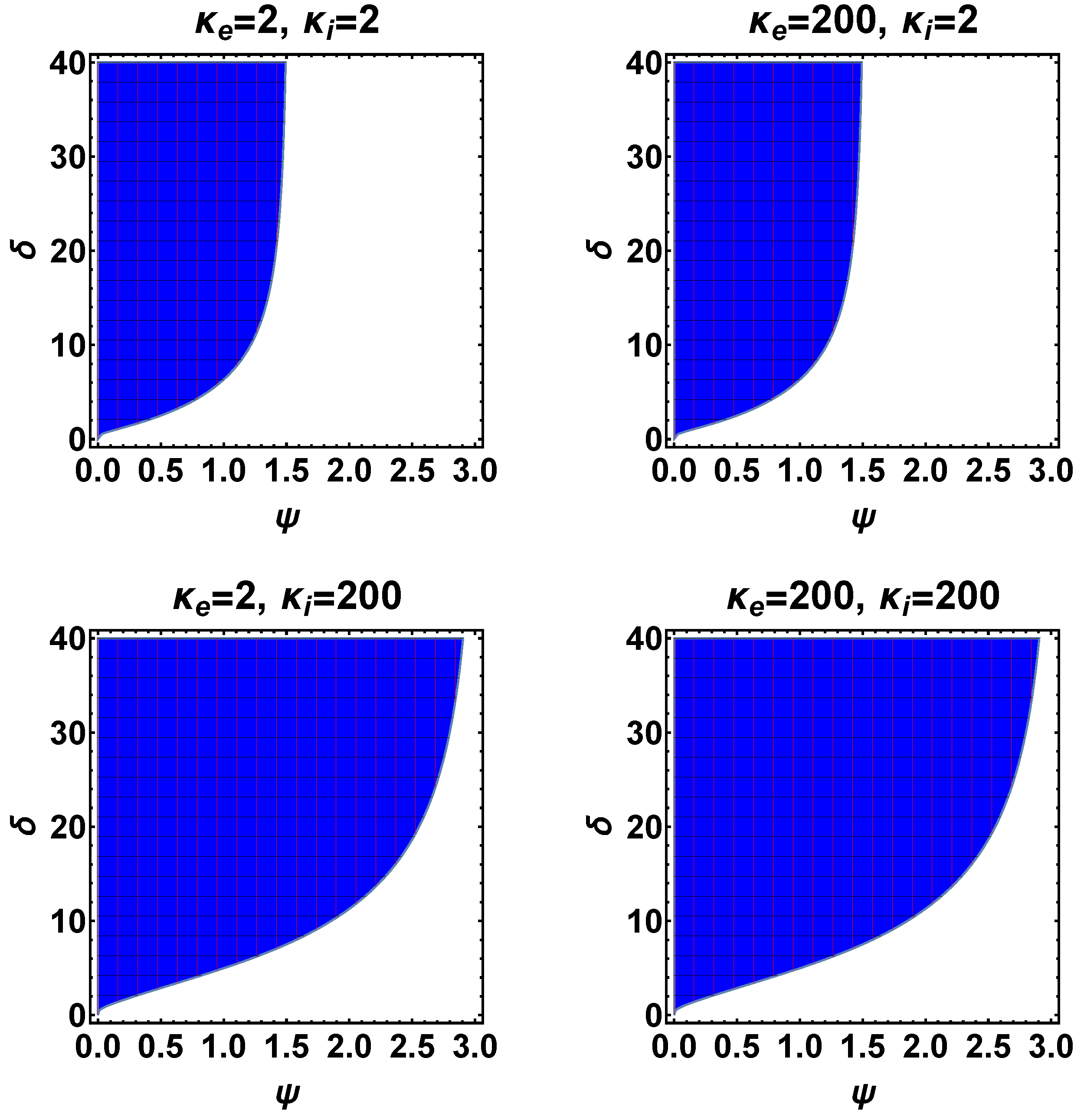
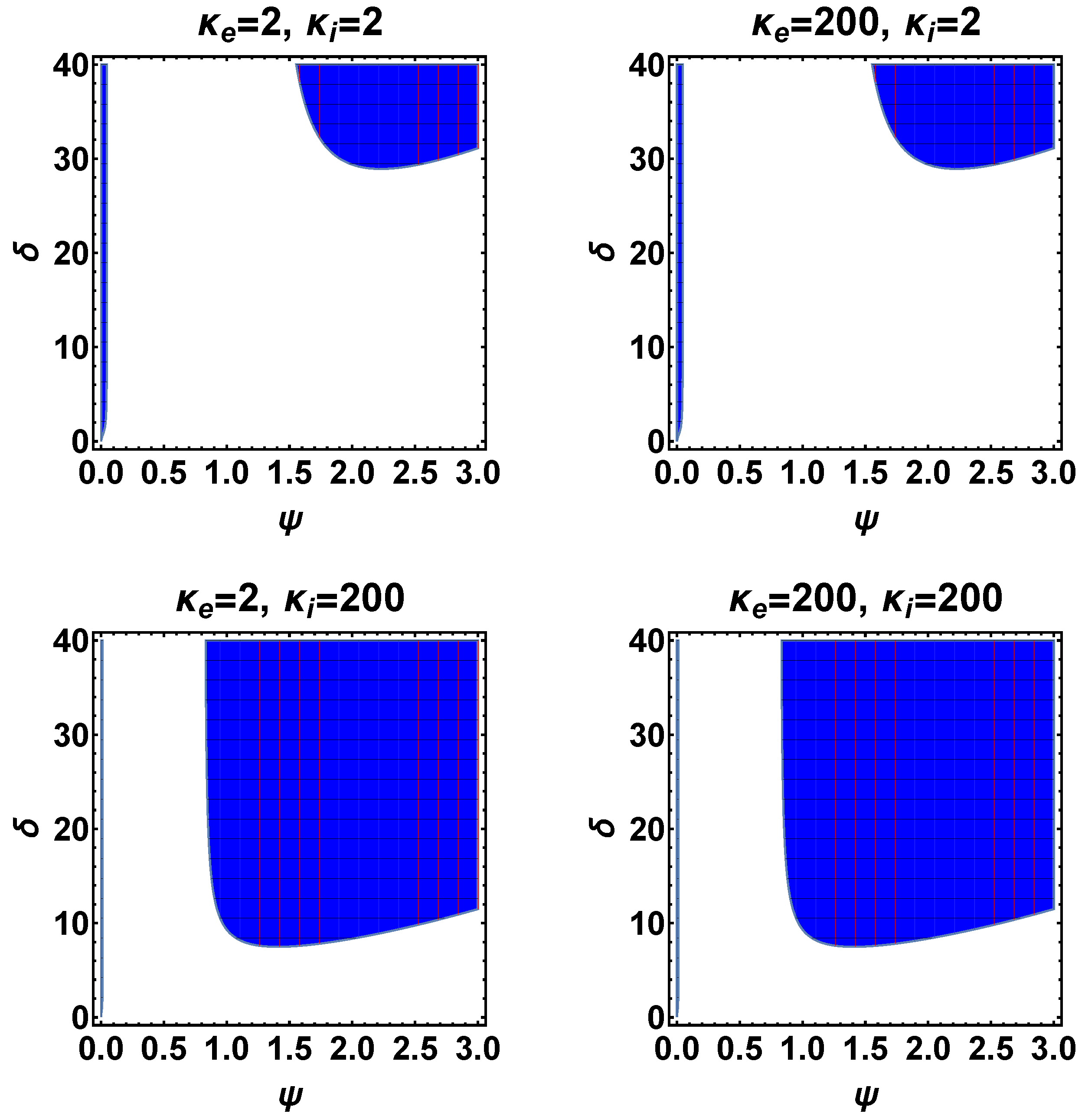
Figure 1 and Figure 2, respectively, show the behavior of physically plausible width-amplitude region, $(\delta ,\psi )$, for the above-mentioned four cases with temperature ratio $T_r=0.5$ and $T_r=3$. For $T_i<T_e$, as exemplified by $T_r=0.5$, the region of plausibility for ion holes shows a clear demarkation—see Figure 1, blue-shaded domains, which correspond to the plausibility condition versus white areas, which indicate forbidden zone. As the ion temperature exceeds that of the electrons $T_i>T_e$ (or specifically $T_r\ge 1$), on the other hand, the physical plausibility condition undergoes a dramatic change, as Figure 2 shows. In specific, a new branch of physically plausible region splits from the main domain, as exemplified by Figure 2. This suggests that the ion-to-electron temperature ratio plays a pivotal role. Henceforth, we refer to the narrow vertical blue strip corresponding to the lower amplitude region, shown in Figure 2, as Region 1 and the main higher amplitude domain, color-coded in blue, Region 2. Note that all four different cases (i–iv) show qualitatively similar features in terms of the overall pattern of plausible versus forbidden parameter space. For this reason we focus on case (i) in order to further investigate the parametric dependence on the behavior of IHs.

3.1. Effects of Potential on IHs

3.1.1. $T_i<T_e$

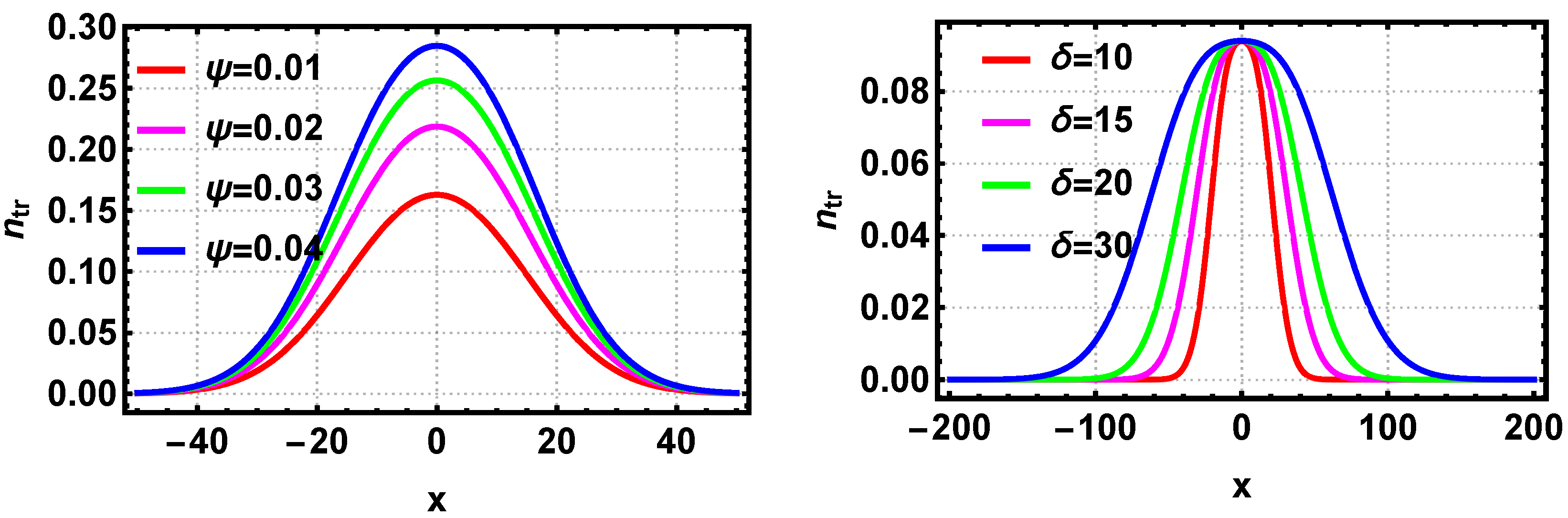
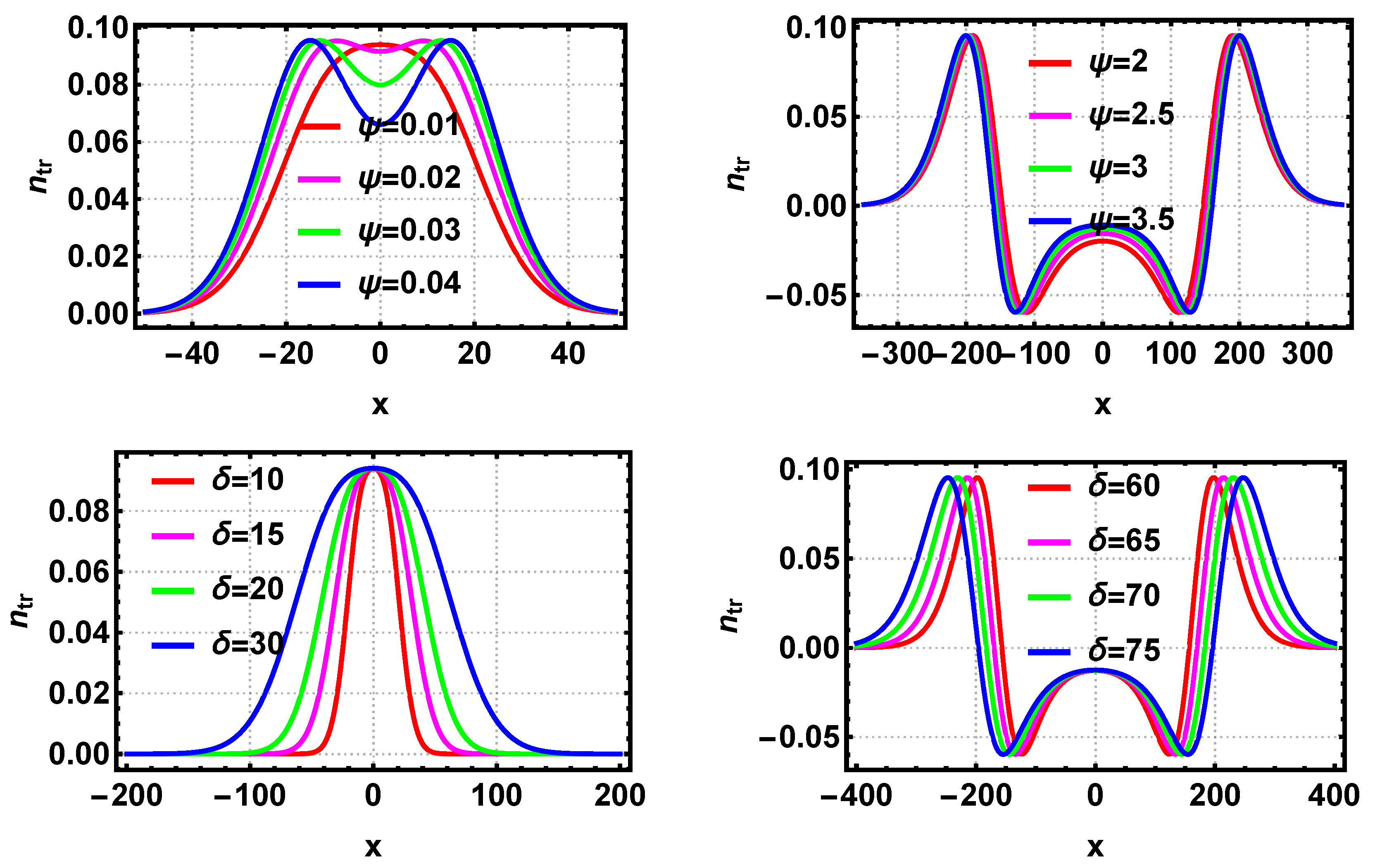
One of the key quantities that defines the BGK equilibria is the trapped particle density. Figure 3 depicts the dependence of trapped ion density on the width and amplitude of the potential when both ions and electrons are suprathermal. The left panel of Figure 3 displays the dependence of trapped ion density for various values of wave amplitude when the electrons have twice the temperature of ions. It can be seen that as the amplitude of the wave-potential increases, the maximum of the trapped density distribution also increases. The right panel shows the influence of wave potential width on the trapped ion density. It is seen that the width controls the spatial spread of trapped ion density. The solitary wave amplitude determines the maximum velocity of the trapped particles, while the width controls how many particles can be trapped in order to sustain the BGK equilibrium.

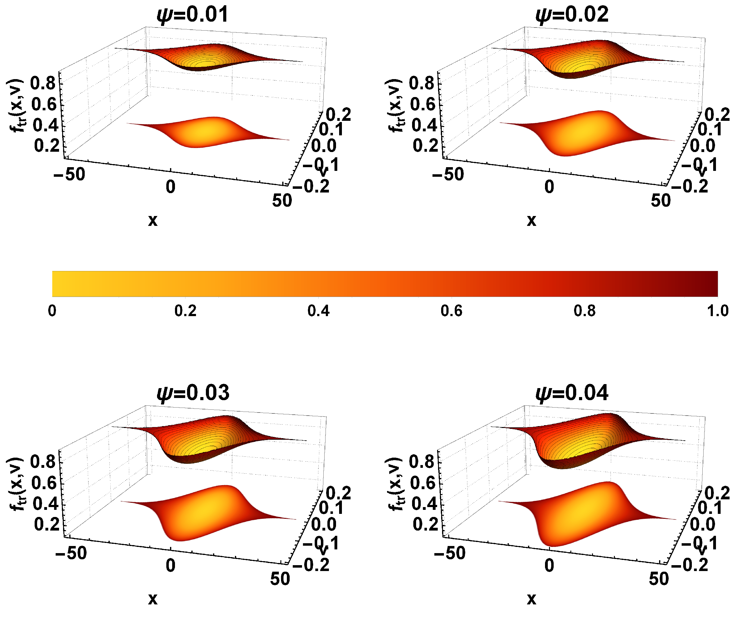
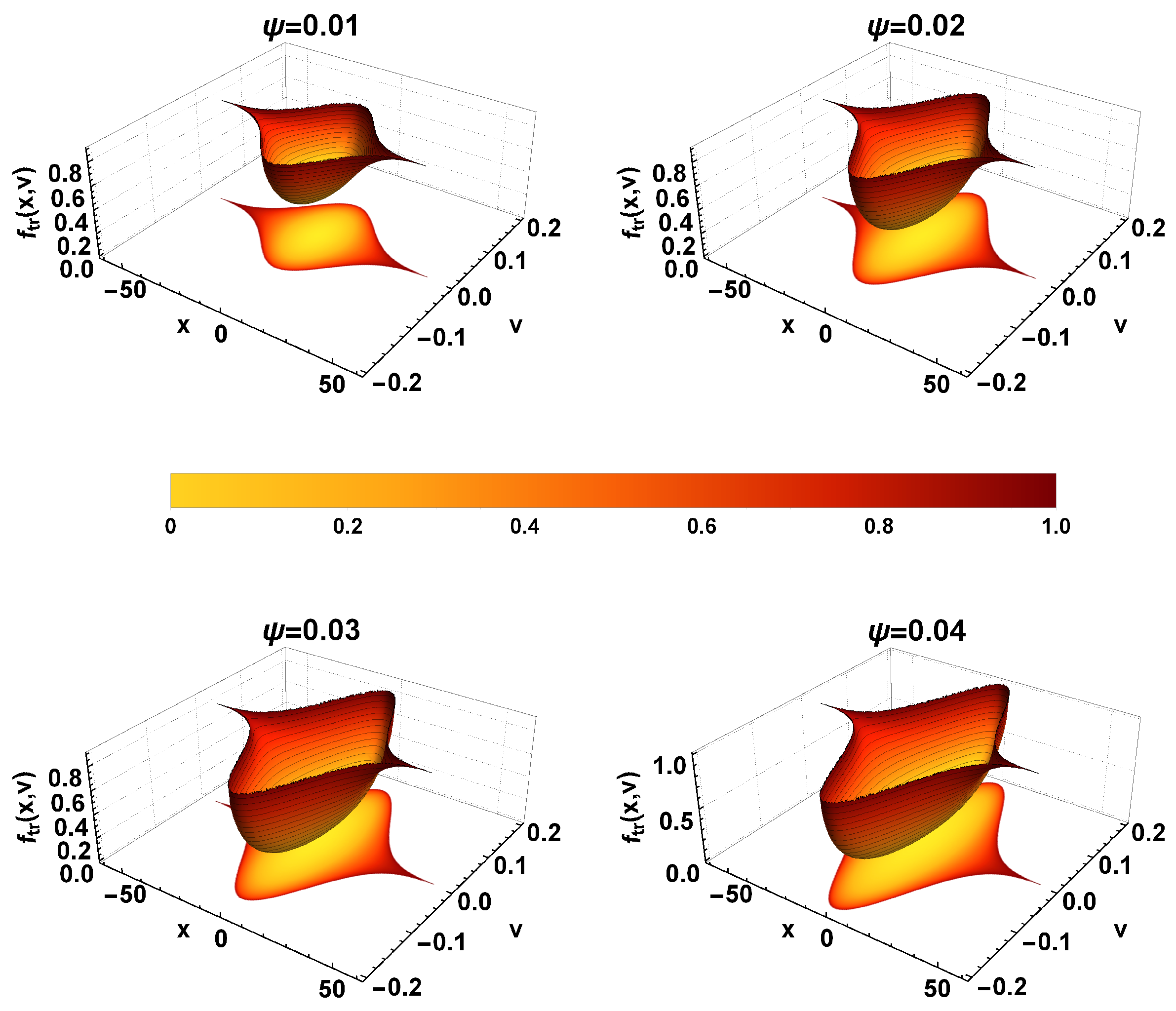
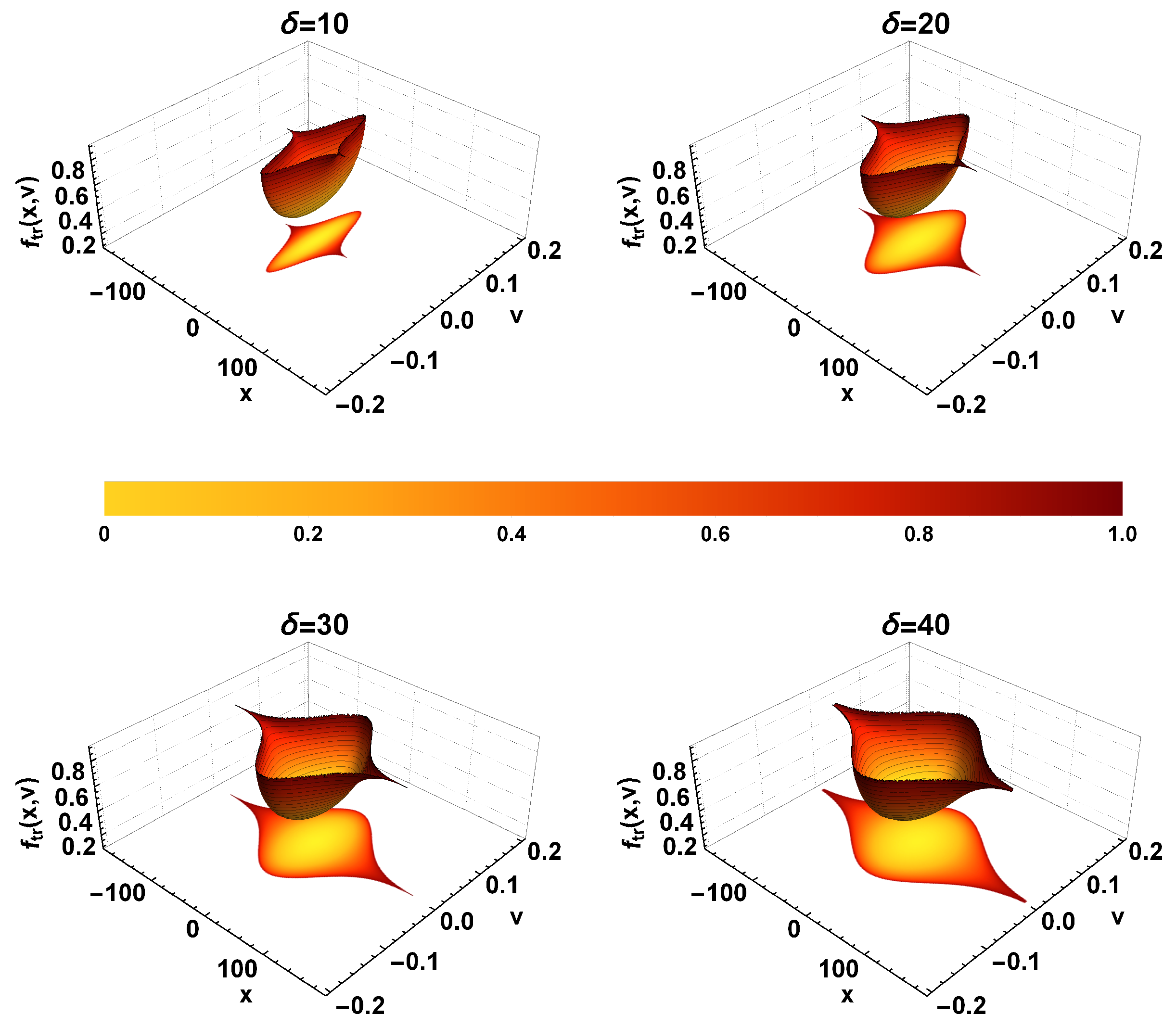
The influence of wave potential amplitude on the BGK equilibrium can be seen in Figure 4, where the trapped ion distribution function is plotted for different values of $\psi$, for fixed $T_r$ and $\delta$. It is seen that $f_{tr}(x,v)$ gets stretched along v axis as the amplitude $\psi$ increases. In order to aid the visualization we also plotted the two-dimensional projection of $f_{tr}$ underneath the surface plots of the trapped-particle distribution.

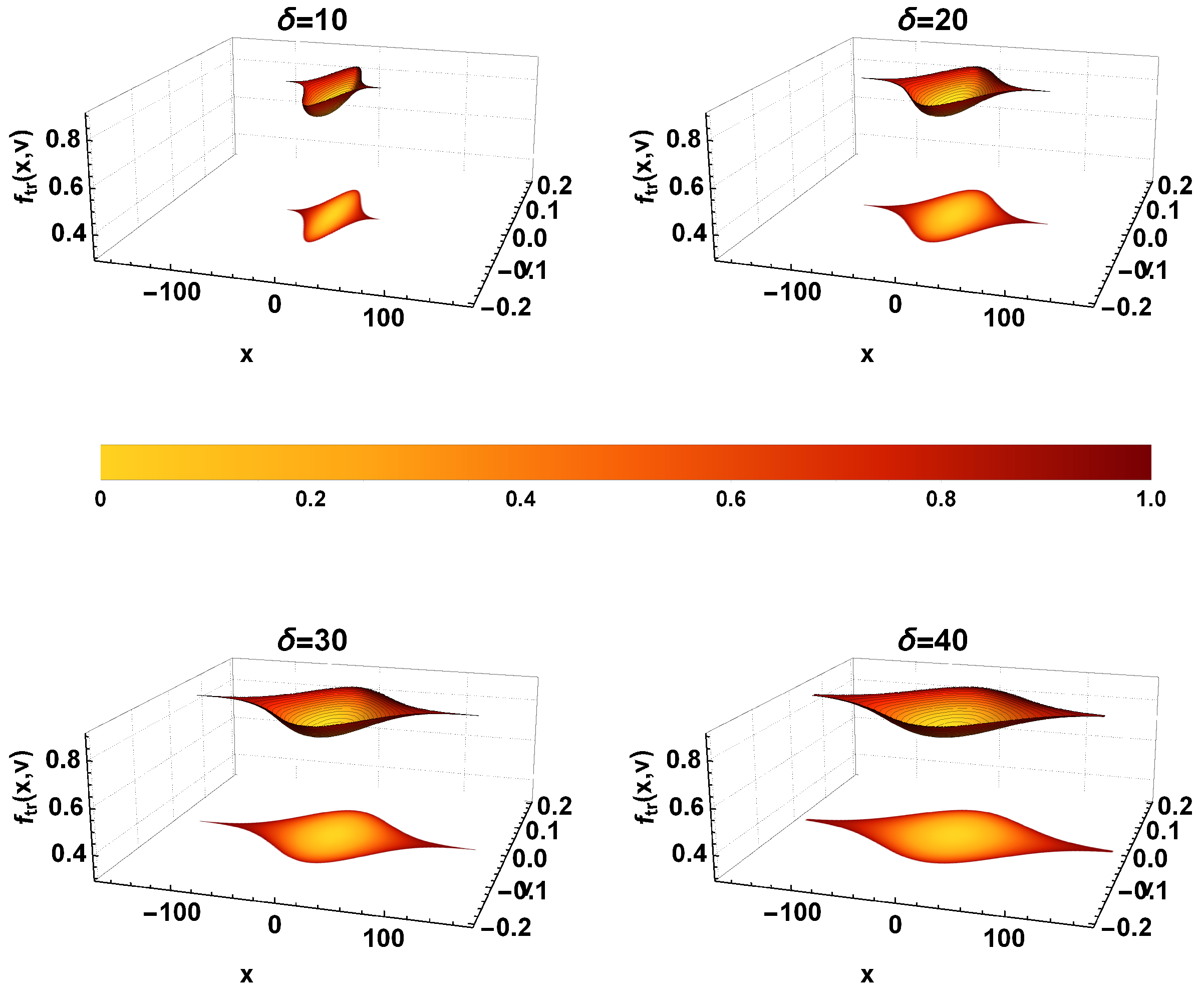
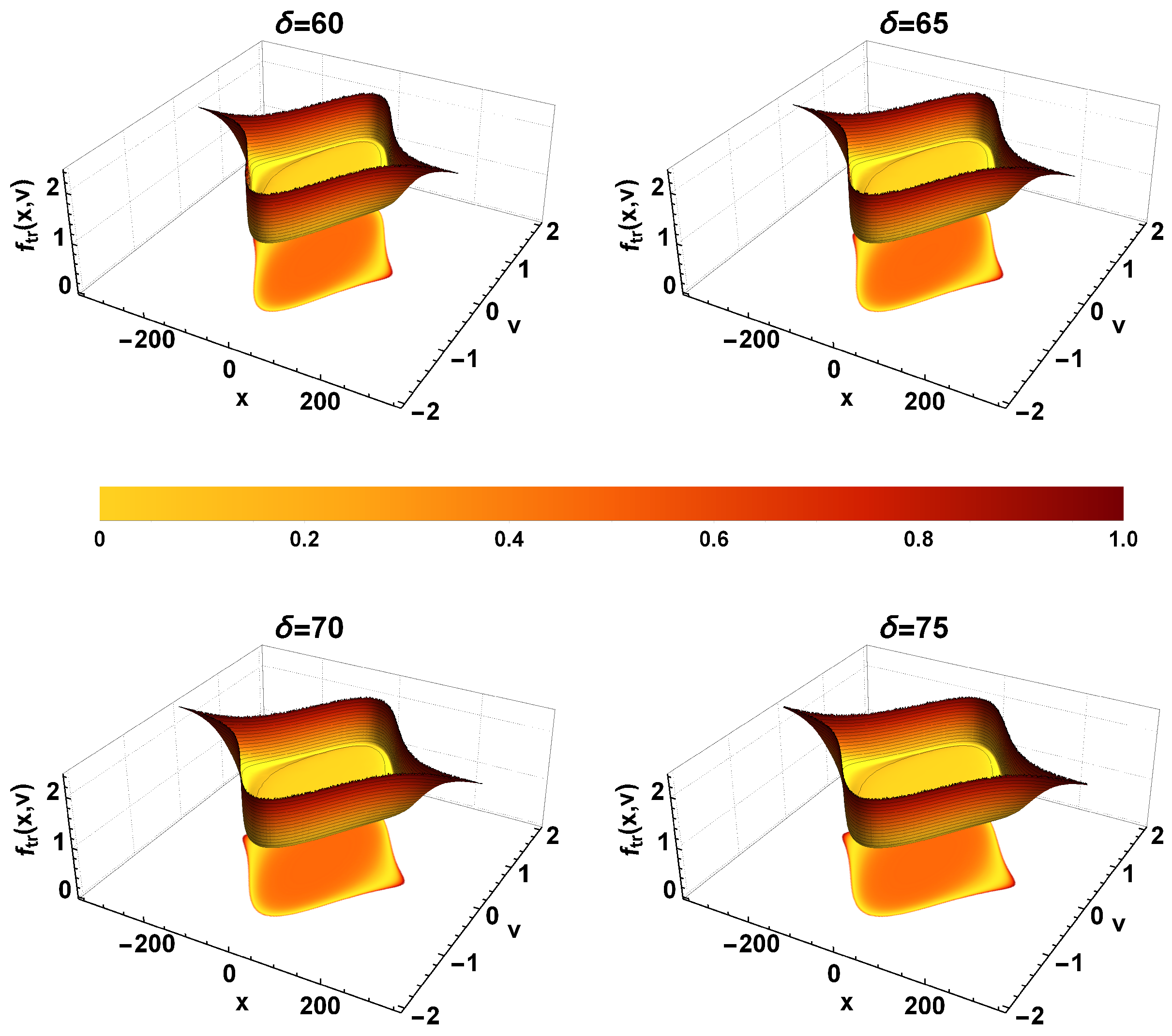
Figure 5 demonstrates the dependence of trapped ion distribution function on varying $\delta$, while keeping $\psi$ and $T_r$ as fixed. For this case, $f_{tr}$ is stretched along x axis, which is consistent with Figure 3, where it is shown that the trapped density broadens as $\delta$ increases. The elongation of $f_{tr}$ along x axis as $\delta$ increases is thus predicted by the behavior of $n_{tr}$. However, the stretching of $f_{tr}$ along v axis, as shown in Figure 4, could not have been predicted on the basis of trapped density analysis.

3.1.2. $T_i>T_e$

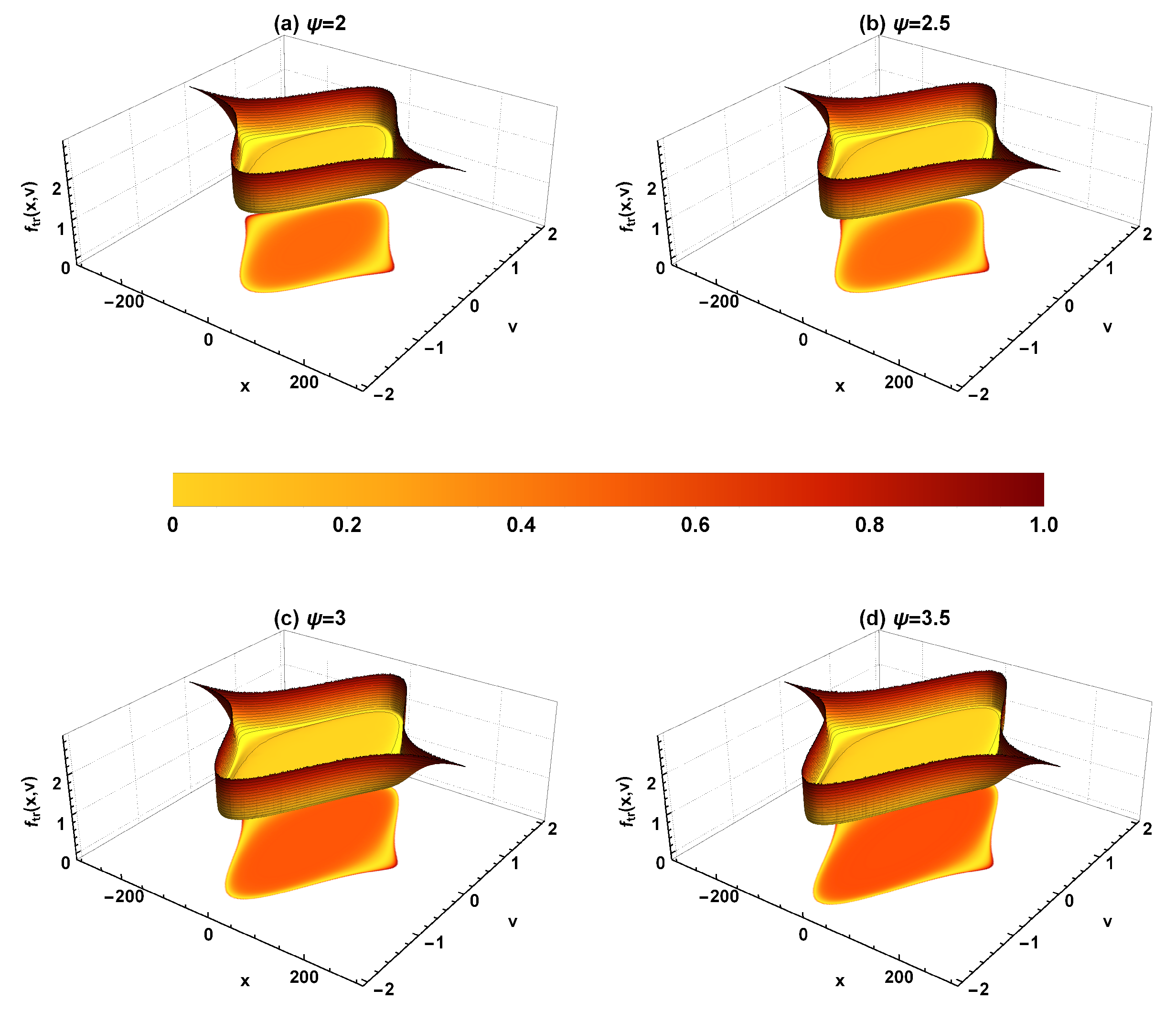
We next consider $T_r=3$ to investigate the phase space structure of IHs when the ion temperature is higher than the electron temperature. As seen in Figure 2, the width-amplitude plot for this case shows Region 1 and Region 2 for the existence of BGK IH equilibria. Thus, we consider the amplitudes and widths from these regions separately in order to examine the behavior IHs. Figure 6 shows the behavior of trapped ion density with the amplitude and width of the wave potential corresponding to Region 1 (left panels) and Region 2 (right panels). Figure 6 demonstrates that the lower amplitude wave potentials (Region 1) have a similar response to the trapped ion density that we have seen for $T_i<T_e$. However, the trapped ion density shows an extreme behavior when the wave potential amplitude is high (Region 2). Despite the width and amplitude from the allowed region, the trapped density delves into negative values that are physically improbable. A similar distribution of trapped density is generally displayed if the stretched solitary wave’s potential generates the BGK equilibria [43]. Figure 7, Figure 8, Figure 9 and Figure 10 depict the corresponding phase space characteristics of the IHs for the cases that are shown in Figure 6. It is seen that the left panels of Figure 7 and Figure 9 show similar behavior as compared to the case of a lower temperature ratio; this indicates that the temperature ratio does not have an explicit dependence on the characteristics of IHs.

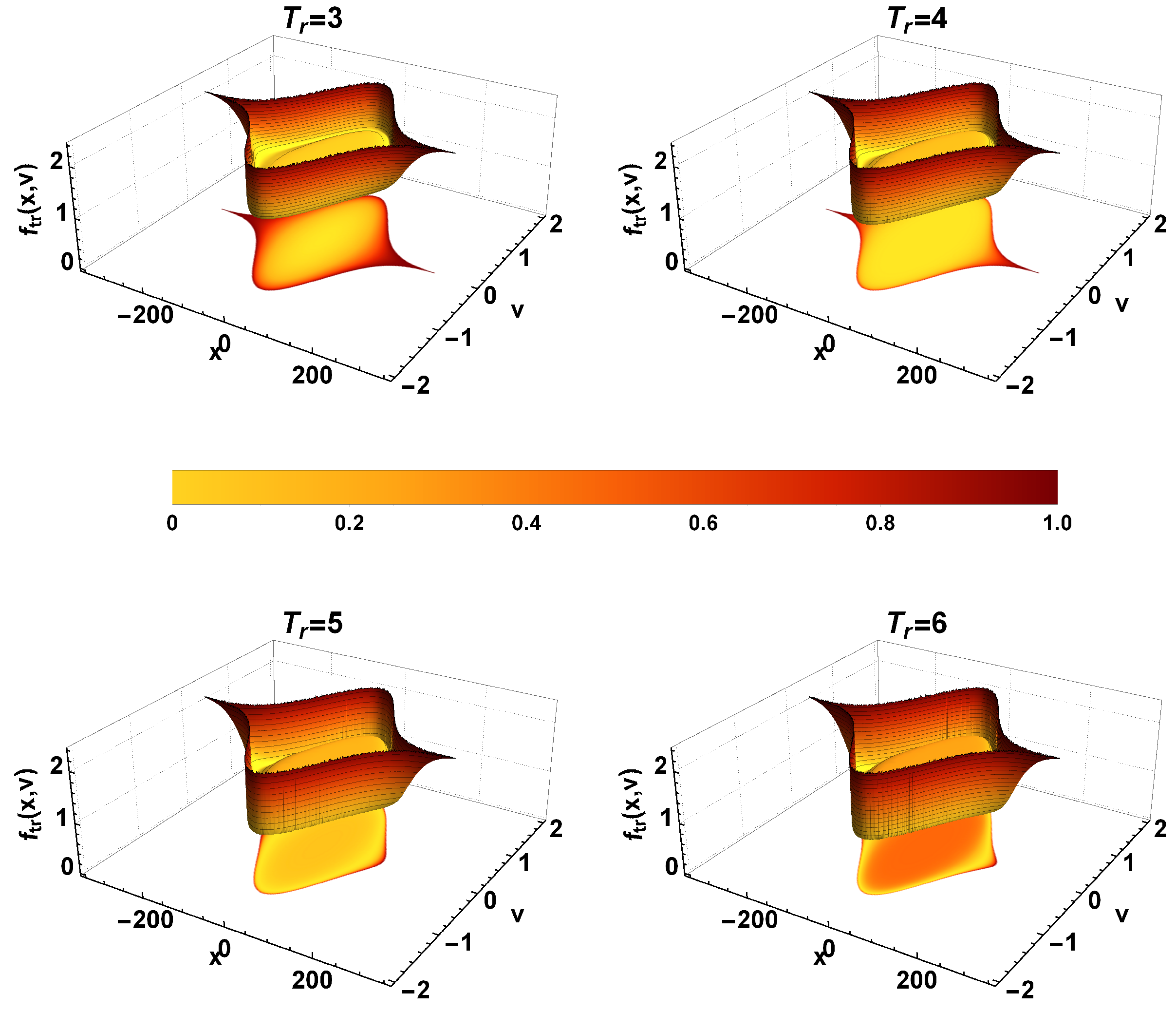
In contrast, the right panels of the Figure 6 and their corresponding phase-space distribution shown in Figure 8 and Figure 10 exhibit a different behavior. Such a trapped density distribution and phase space portrayal are a general characteristics of the stretched solitary wave. In Figure 8 and Figure 10, unlike a smooth minimum, a small local maximum appears at the center of trapped ion phase space distribution function. A small hump in the phase space is attributed to the momentum transfer between the electrons to the trapped ions [43]. When the temperature ratio ($T_r$) is large, i.e., when ions have a higher temperature and the wave potential depth is correspondingly high, a wider range of phase space is available for the electrons to interact with the potential. As the interaction of the electrons is most efficient at the center of the potential, the largest transfer of momentum causes the ions to bunch, which is depicted as a hump in the phase space. This transfer of momentum translates to the such kind of trapped ion density distribution.

3.2. Effects of Temperature Ratio, $T_r$

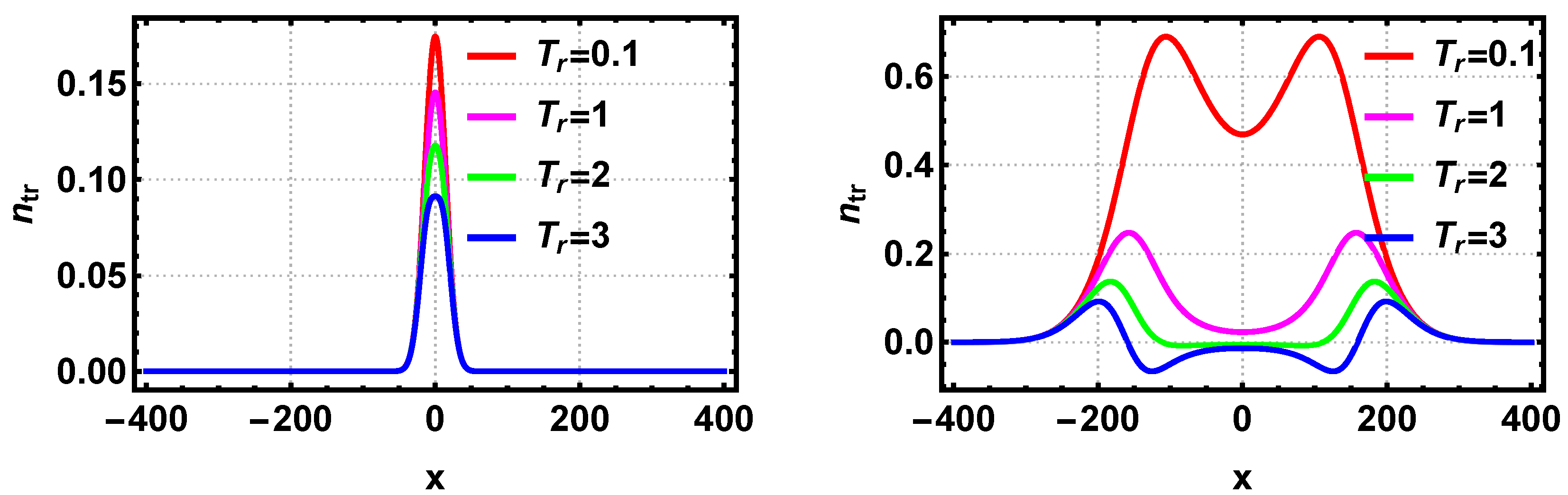
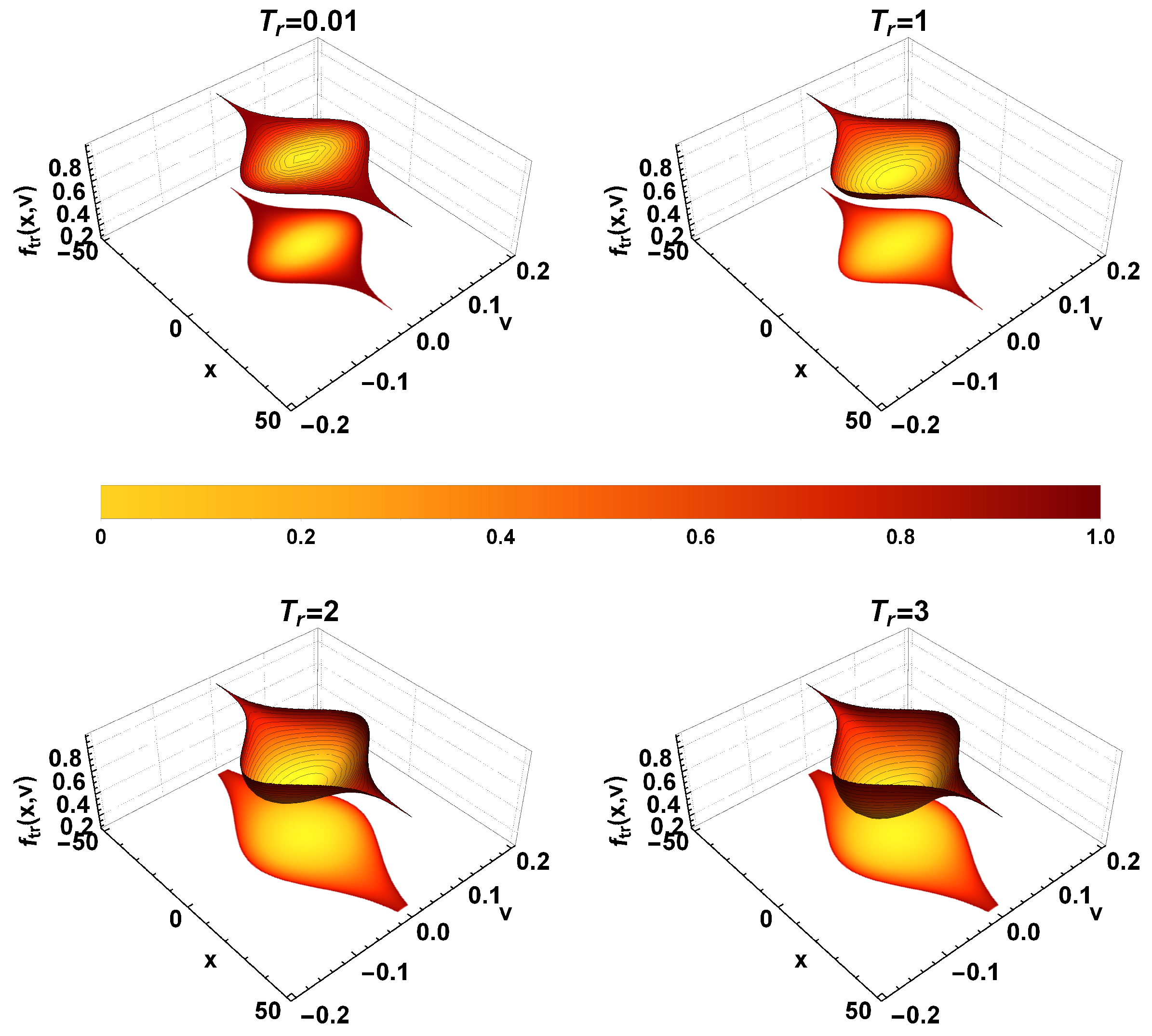
We have seen that the ion-to-electron temperature ratio is a critical factor that determines the structure of IHs. We investigate the effects of $T_r$ more systematically. Figure 11 depicts the role of temperature ratio in determining the characteristics of BGK IH equilibria. The left panel shows the case for extremely low amplitudes and widths from Region 1, while the right panel shows the case for higher amplitudes and widths from Region 2. If the wave potential is constant, a monotonic increase in the temperature ratio decreases the trapped density, indicating that the colder the electrons, the lower the trapped ion density. This might be due to increased ion-electron interactions. Physically, as the ion temperature is higher, a smaller potential cannot trap highly energetic ions, or equivalently, the BGK equilibrium does not demand a higher density of trapped particles in order to sustain the equilibria. The phase space portrait of this scenario is shown in Figure 12. The trapped ion distribution function displays a higher depth for higher temperature ratio. Thus, a BGK ion hole will exhibit more pronounced depth if the ion-to-electron temperature ratio is high. It should be noted that a similar effect is not displayed by any other parameters than the temperature ratio. Thus, the temperature ratio holds the key to decide the depth of the BGK IH equilibria. Physically, as the temperature ratio works as a negative catalyst to the trapped density, the trapped ions have a wider space to oscillate inside the potential, creating a deeper hole.

The right panel of Figure 11 shows the scenario when the amplitude and potential are higher. The unusual nature observed in the earlier cases repeats here also. The corresponding phase-space portrait, Figure 13, also shows a similar effect. It can be seen that as the temperature ratio $T_r$ increases, a small hump emerges in the trapped ion distribution function. The plot of trapped density shows that the temperature ratio facilitates the momentum transfer, generating the hump in the trapped ion distribution function.

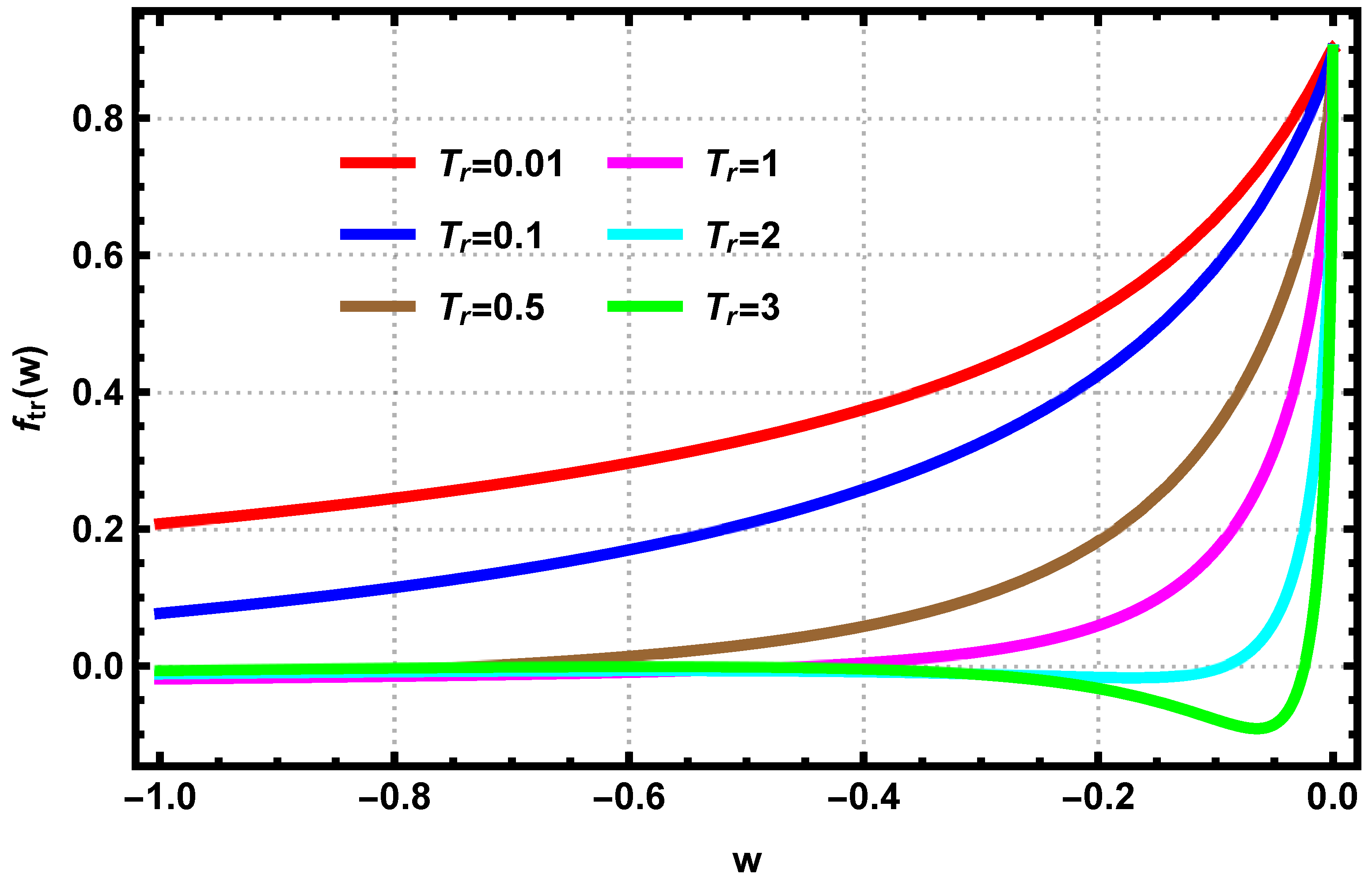
A general inspection of the width-amplitude relation shows that a forbidden band is created in the width-amplitude plot at specific temperature ratios, $T_r$. Figure 14 reveals that this puzzling phenomenon is due to the sudden generation of a saddle point in the energy space. Again a probable physical explanation is the interaction of electrons with ions. Thus, this proves that the wave potential should be strong enough to hold the required trapped density, or else, the ions will get untrapped. Consequently, the equilibria will be dissolved, leading to the violation of the heteroclinic property of the phase-space. Thus, it opens a piece of direct evidence that there is a transfer of momentum taking place between the electron and ions.

4. Conclusions

This paper probes the structural characteristics of BGK ion holes based on the theoretical formulation by Aravindakshan et al. [12]. From the comparative study of width-amplitude relationship for IHs for plasmas with different particle distributions, we uncovered that a forbidden band of amplitude is present as the temperature of ions exceeds that of the electrons. From the analysis of trapped ion distribution function, mathematically it turns out that the reason stems from the non-differential nature of the electron density. Hence, we propose that this is due to the interaction of electrons with the wave potential. The study of characteristics of IHs leads us to conclude that the width of the potential decides the number density of trapped particles required to form a BGK ion hole equilibria. Also, when the ion-to-electron temperature ratio increases, the depth of the holes increases. We argue that due to the thermal energy acquired by the ions when they are at high temperatures, these trapped ions oscillate inside the potential with a higher amplitude. The characteristics of ion holes lead us towards more radical thoughts on the fundamental nature of ion-electron interactions, momentum, energy transfer, the plasma distribution function’s role, etc., in BGK equilibria’s stability. Thus, this paper finally opens a path to explore such fundamental yet crucial questions that the space plasma community to ponder.

References

- Matsumoto, H.; Kojima, H.; Miyatake, T.; Omura, Y.; Okada, M.; Nagano, I.; Tsutsui, M. Electrostatic solitary waves (ESW) in the magnetotail: BEN wave forms observed by GEOTAIL. Geophys. Res. Lett. 1994, 21, 2915–2918. [Google Scholar] [CrossRef]
- Ergun, R.; Carlson, C.; Muschietti, L.; Roth, I.; McFadden, J. Properties of fast solitary structures. Nonlinear Process. Geophys. 1999, 6, 187–194. [Google Scholar] [CrossRef]
- McFadden, J.; Carlson, C.; Ergun, R.; Mozer, F.; Muschietti, L.; Roth, I.; Moebius, E. FAST observations of ion solitary waves. J. Geophys. Res. Space Phys. 2003, 108, 8018. [Google Scholar] [CrossRef]
- Liemohn, M.W.; Johnson, B.C.; Fränz, M.; Barabash, S. Mars Express observations of high altitude planetary ion beams and their relation to the “energetic plume” loss channel. J. Geophys. Res. Space Phys. 2014, 119, 9702–9713. [Google Scholar] [CrossRef] [Green Version]
- Kakad, A.; Kakad, B.; Anekallu, C.; Lakhina, G.; Omura, Y.; Fazakerley, A. Slow electrostatic solitary waves in earth’s plasma sheet boundary layer. J. Geophys. Res. Space Phys. 2016, 121, 4452–4465. [Google Scholar] [CrossRef]
- Holmes, J.; Ergun, R.; Newman, D.; Ahmadi, N.; Andersson, L.; Le Contel, O.; Torbert, R.; Giles, B.; Strangeway, R.; Burch, J. Electron Phase-Space Holes in Three Dimensions: Multispacecraft Observations by Magnetospheric Multiscale. J. Geophys. Res. Space Phys. 2018, 123, 9963–9978. [Google Scholar] [CrossRef]
- Wang, R.; Vasko, I.; Mozer, F.; Bale, S.; Artemyev, A.; Bonnell, J.; Ergun, R.; Giles, B.; Lindqvist, P.A.; Russell, C.; et al. Electrostatic turbulence and Debye-scale structures in collisionless shocks. Astrophys. J. Lett. 2020, 889, L9. [Google Scholar] [CrossRef] [Green Version]
- Saeki, K.; Michelsen, P.; Pécseli, H.; Rasmussen, J.J. Formation and coalescence of electron solitary holes. Phys. Rev. Lett. 1979, 42, 501. [Google Scholar] [CrossRef]
- Singh, K.; Kakad, A.; Kakad, B.; Saini, N.S. Evolution of ion acoustic solitary waves in pulsar wind. Mon. Not. R. Astron. Soc. 2021, 500, 1612–1620. [Google Scholar] [CrossRef]
- Bernstein, I.B.; Greene, J.M.; Kruskal, M.D. Exact nonlinear plasma oscillations. Phys. Rev. 1957, 108, 546. [Google Scholar] [CrossRef] [Green Version]
- Soni, P.K.; Aravindakshan, H.; Kakad, B.; Kakad, A. Nonlinear particle trapping by coherent waves in thermal and nonthermal plasmas. Phys. Scr. 2021, 96, 105604. [Google Scholar] [CrossRef]
- Aravindakshan, H.; Yoon, P.H.; Kakad, A.; Kakad, B. Theory of ion holes in space and astrophysical plasmas. Mon. Not. R. Astron. Soc. Lett. 2020, 497, L69–L75. [Google Scholar] [CrossRef]
- Aravindakshan, H.; Kakad, A.; Kakad, B. Bernstein-Greene-Kruskal theory of electron holes in superthermal space plasma. Phys. Plasmas 2018, 25, 052901. [Google Scholar] [CrossRef]
- Aravindakshan, H.; Kakad, A.; Kakad, B. Effects of wave potential on electron holes in thermal and superthermal space plasmas. Phys. Plasmas 2018, 25, 122901. [Google Scholar] [CrossRef]
- Boström, R.; Gustafsson, G.; Holback, B.; Holmgren, G.; Koskinen, H.; Kintner, P. Characteristics of solitary waves and weak double layers in the magnetospheric plasma. Phys. Rev. Lett. 1988, 61, 82. [Google Scholar] [CrossRef]
- Schamel, H. Stationary solutions of the electrostatic Vlasov equation. Plasma Phys. 1971, 13, 491. [Google Scholar] [CrossRef]
- Bujarbarua, S.; Schamel, H. Theory of finite-amplitude electron and ion holes. J. Plasma Phys. 1981, 25, 515–529. [Google Scholar] [CrossRef]
- Schamel, H. Electron holes, ion holes and double layers: Electrostatic phase space structures in theory and experiment. Phys. Rep. 1986, 140, 161–191. [Google Scholar] [CrossRef]
- Hutchinson, I.H. Electron holes in phase space: What they are and why they matter. Phys. Plasmas 2017, 24, 055601. [Google Scholar] [CrossRef]
- Chen, L.J.; Thouless, D.J.; Tang, J.M. Bernstein–Greene–Kruskal solitary waves in three-dimensional magnetized plasma. Phys. Rev. E 2004, 69, 055401. [Google Scholar] [CrossRef] [Green Version]
- Ma, C.y.; Summers, D. Formation of power-law energy spectra in space plasmas by stochastic acceleration due to whistler-mode waves. Geophys. Res. Lett. 1998, 25, 4099–4102. [Google Scholar] [CrossRef] [Green Version]
- Yoon, P.H.; Rhee, T.; Ryu, C.M. Self-consistent generation of superthermal electrons by beam-plasma interaction. Phys. Rev. Lett. 2005, 95, 215003. [Google Scholar] [CrossRef] [Green Version]
- Tao, X.; Lu, Q. Formation of electron kappa distributions due to interactions with parallel propagating whistler waves. Phys. Plasmas 2014, 21, 022901. [Google Scholar] [CrossRef]
- Yoon, P.H.; Livadiotis, G. Nonlinear wave–particle interaction and electron kappa distribution. In Kappa Distributions; Elsevier: Amsterdam, The Netherlands, 2017; pp. 363–398. [Google Scholar] [CrossRef]
- Elkamash, I.; El-Hanbaly, A. The effect of κ-distributed trapped electrons on fully nonlinear electrostatic solitary waves in an electron–positron-relativistic ion plasma. J. Phys. A Math. Theor. 2021, 54, 065701. [Google Scholar] [CrossRef]
- Schwadron, N.A.; Dayeh, M.; Desai, M.; Fahr, H.; Jokipii, J.R.; Lee, M.A. Superposition of stochastic processes and the resulting particle distributions. Astrophys. J. 2010, 713, 1386. [Google Scholar] [CrossRef]
- Livadiotis, G.; McComas, D. The influence of pick-up ions on space plasma distributions. Astrophys. J. 2011, 738, 64. [Google Scholar] [CrossRef]
- Yoon, P.H. Electron kappa distribution and quasi-thermal noise. J. Geophys. Res. Space Phys. 2014, 119, 7074–7087. [Google Scholar] [CrossRef]
- Zank, G.; Li, G.; Florinski, V.; Hu, Q.; Lario, D.; Smith, C. Particle acceleration at perpendicular shock waves: Model and observations. J. Geophys. Res. Space Phys. 2006, 111. [Google Scholar] [CrossRef] [Green Version]
- Livadiotis, G. Long-term independence of solar wind polytropic index on plasma flow speed. Entropy 2018, 20, 799. [Google Scholar] [CrossRef] [PubMed] [Green Version]
- Encrenaz, T.; Kallenbach, R.; Owen, T.; Sotin, C. The Outer Planets and Their Moons: Comparative Studies of the Outer Planets Prior to the Exploration of the Saturn System by Cassini-Huygens; Springer Science & Business Media: Berlin/Heidelberg, Germany, 2005; Volume 19. [Google Scholar]
- Krimigis, S.; Armstrong, T.; Axford, W.; Cheng, A.; Gloeckler, G.; Hamilton, D.; Keath, E.; Lanzerotti, L.; Mauk, B. The magnetosphere of Uranus: Hot plasma and radiation environment. Science 1986, 233, 97–102. [Google Scholar] [CrossRef]
- Krupp, N. Energetic particles in the magnetosphere of Saturn and a comparison with Jupiter. Space Sci. Rev. 2005, 116, 345–369. [Google Scholar] [CrossRef]
- Espinoza, C.; Stepanova, M.; Moya, P.; Antonova, E.; Valdivia, J. Ion and Electron κ Distribution Functions Along the Plasma Sheet. Geophys. Res. Lett. 2018, 45, 6362–6370. [Google Scholar] [CrossRef]
- Felici, M.; Arridge, C.S.; Coates, A.; Badman, S.V.; Dougherty, M.; Jackman, C.M.; Kurth, W.; Melin, H.; Mitchell, D.G.; Reisenfeld, D.; et al. Cassini observations of ionospheric plasma in Saturn’s magnetotail lobes. J. Geophys. Res. Space Phys. 2016, 121, 338–357. [Google Scholar] [CrossRef] [PubMed] [Green Version]
- Richardson, J.D.; Belcher, J.W.; Garcia-Galindo, P.; Burlaga, L.F. Voyager 2 plasma observations of the heliopause and interstellar medium. Nat. Astron. 2019, 3, 1019–1023. [Google Scholar] [CrossRef]
- Lotekar, A.; Kakad, A.; Kakad, B. Fluid simulation of dispersive and nondispersive ion acoustic waves in the presence of superthermal electrons. Phys. Plasmas 2016, 23, 102108. [Google Scholar] [CrossRef]
- Saini, N.; Kourakis, I.; Hellberg, M. Arbitrary amplitude ion-acoustic solitary excitations in the presence of excess superthermal electrons. Phys. Plasmas 2009, 16, 062903. [Google Scholar] [CrossRef] [Green Version]
- Kakad, A.; Omura, Y.; Kakad, B. Experimental evidence of ion acoustic soliton chain formation and validation of nonlinear fluid theory. Phys. Plasmas 2013, 20, 062103. [Google Scholar] [CrossRef] [Green Version]
- Khain, P.; Friedland, L. A water bag theory of autoresonant Bernstein-Greene-Kruskal modes. Phys. Plasmas 2007, 14, 082110. [Google Scholar] [CrossRef]
- Friedland, L.; Khain, P.; Shagalov, A. Autoresonant phase-space holes in plasmas. Phys. Rev. Lett. 2006, 96, 225001. [Google Scholar] [CrossRef] [Green Version]
- Chen, L.J. Bernstein-Greene-Kruskal Solitary Waves in Collisionless Plasma. Ph.D. Thesis, University of Washington, Seattle, WA, USA, 2002. [Google Scholar]
- Muschietti, L.; Roth, I.; Carlson, C.; Berthomier, M. Modeling stretched solitary waves along magnetic field lines. Nonlinear Process. Geophys. 2002, 9, 101–109. [Google Scholar] [CrossRef]
Figure 1.
The width-amplitude relation for different configuration of ion and electron distribution function is shown for temperature ratio, . The blue-shaded regions correspond to the parameter space that permits the existence of ion holes.
Figure 2.
The width-amplitude relation for different configuration of ion and electron distribution function is shown for temperature ratio, .
Figure 3.
The dependence of trapped ion density for different and is shown. The left panel shows the case for different , for fixed and . The right panel shows the case for different keeping the and constant.
Figure 4.
Three-dimensional structure of the trapped ion distribution function versus x and v, for different values of , while keeping and as fixed. The color bar indicates the density. The two-dimensional projection of is displayed underneath the surface plot of the trapped ion distribution function.
Figure 5.
The same as Figure 4, except that the potential width is varied, while keeping and as constants.
Figure 6.
The characteristics of trapped ion density for different and are shown. The top panels show the case for different keeping the and constant. In the top left panel, the values of are taken from Region 1, and is assumed to be 10. In the top-right panel, the values of are taken from Region 2, and is assumed to be 60. The bottom panels show the case for different keeping the and constant. In the bottom left panel, is assumed to be 0.01 (from Region 1), whereas in the bottom right panel is assumed to be 2 (from Region 2) for different values of .
Figure 7.
The trapped ion distribution function versus x and v, as well as 2D projection, for different values of , and for fixed and .
Figure 8.
The same as Figure 7, except that the choice of and designate Region 2. For each panel, a small hump at the center of the phase space distribution can be observed.
Figure 9.
The trapped ion distribution function for different keeping and as constants. The values for width and amplitude are from Region 1.
Figure 10.
The trapped ion distribution function for different keeping and as constants. The input amplitude represent Region 2. The central hump characterizes the phase space distribution for each case.
Figure 11.
The characteristics of trapped ion density for different is shown keeping and constant. The left panel shows the case for different keeping and as fixed, i.e., from Region 1. The right panel show the case for different keeping and as constants, i.e., from Region 2.
Figure 12.
The trapped ion distribution function versus x and v, as well as 2D projection, for different values of , keeping and constants. The values for width and amplitude are from Region 1.
Figure 13.
The same as Figure 12, except that and are used. The input parameters are from Region 2. The central hump characterizes the phase space distribution for all the cases considered here.
Figure 14.
The characteristics of trapped ion distribution function for different keeping and as constants. The emergence of saddle point after crosses the threshold, , denotes the occurrence of forbidden gap in the width-amplitude plot.
Publisher’s Note: MDPI stays neutral with regard to jurisdictional claims in published maps and institutional affiliations. |
© 2021 by the authors. Licensee MDPI, Basel, Switzerland. This article is an open access article distributed under the terms and conditions of the Creative Commons Attribution (CC BY) license (https://creativecommons.org/licenses/by/4.0/).
Share and Cite
MDPI and ACS Style
Aravindakshan, H.; Kakad, A.; Kakad, B.; Yoon, P.H. Structural Characteristics of Ion Holes in Plasma. Plasma 2021, 4, 435-449. https://0-doi-org.brum.beds.ac.uk/10.3390/plasma4030032
AMA Style
Aravindakshan H, Kakad A, Kakad B, Yoon PH. Structural Characteristics of Ion Holes in Plasma. Plasma. 2021; 4(3):435-449. https://0-doi-org.brum.beds.ac.uk/10.3390/plasma4030032
Chicago/Turabian StyleAravindakshan, Harikrishnan, Amar Kakad, Bharati Kakad, and Peter H. Yoon. 2021. "Structural Characteristics of Ion Holes in Plasma" Plasma 4, no. 3: 435-449. https://0-doi-org.brum.beds.ac.uk/10.3390/plasma4030032