
Particle Propagation and Electron Transport in Gases

1
Aeronautics and Astronautics, Stanford University, 496 Lomita Mall, Stanford, CA 94305, USA
2
Division of Electronics for Informatics, Graduate School of Information Science and Technology, Hokkaido University, Sapporo 060-0814, Japan
3
Dipartimento di Chimica, Università degli Studi di Bari, Via Orabona 4, 70126 Bari, Italy
4
Istituto per la Scienza e Tecnologia dei Plasmi, National Research Council of Italy—CNR, 70126 Bari, Italy
*
Authors to whom correspondence should be addressed.
Plasma 2024, 7(1), 121-145; https://0-doi-org.brum.beds.ac.uk/10.3390/plasma7010009
Submission received: 3 January 2024
/
Revised: 2 February 2024
/
Accepted: 9 February 2024
/
Published: 16 February 2024
Abstract
:In this review, we detail the commonality of mathematical intuitions that underlie three numerical methods used for the quantitative description of electron swarms propagating in a gas under the effect of externally applied electric and/or magnetic fields. These methods can be linked to the integral transport equation, following a common thread much better known in the theory of neutron transport than in the theory of electron transport. First, we discuss the exact solution of the electron transport problem using Monte Carlo (MC) simulations. In reality we will go even further, showing the interpretative role that the diagrams used in quantum theory and quantum field theory can play in the development of MC. Then, we present two methods, the Monte Carlo Flux and the Propagator method, which have been developed at this moment. The first one is based on a modified MC method, while the second shows the advantage of explicitly applying the mathematical idea of propagator to the transport problem.
1. Introduction
The goal of kinetic theory is the modeling of a gas (or plasma, or any system made up of a large number of particles) by a distribution function in the particle phase space. This phase space includes the position and velocity coordinates, but also microscopic variables, which describe the “state” of the particles. In this respect, several textbooks and review papers have been devoted to describe the mathematical foundations of kinetic theory of gases and plasmas [1,2,3,4,5,6]. The need to create mathematical models of ionized gases at low temperatures has also been felt for many decades. In fact, the applications of these systems are numerous and qualitatively important and range from the detection of ionizing radiation to the production of new materials, to medicine, and the emission of light [7]. It is not possible to build a reliable model of a low-temperature ionized gas without a detailed description of electron transport and kinetics. For this reason, a gigantic literature was born and developed, including thousands of works, on the development of numerical calculation methods that allow us to calculate the quantities that describe these phenomena [8,9,10].
Since the density of electrons in a weakly ionized gas is much lower than that of the neutral background gas, their behaviour is governed by externally applied fields (electric or magnetic) and by the various collisions that they undergo with the molecules or atoms of the neutral gas. Under these assumptions, it follows that the motion of electrons in the phase space can be described by a single particle distribution function under the linear electron Boltzmann equation (EBE) [11,12]:
where , , and t are the configuration space coordinates, velocity space coordinates, and time, respectively, e is the elementary charge, m is the electron mass, is the electric field, and is the collision term that takes into account electron collisions with the neutral background gas atoms or molecules. For the category of problems in question, this equation becomes linear, since in a very low ionized gas, the interaction between charged particles can be neglected. In this review, in fact, we focus on the linear Boltzmann equation where self-collisions of electrons are neglected. More complex transport equations consider the interaction between charged particles. This interaction can be included with different methods, where one consists of describing it at the micro-mechanical level rather than as an instantaneous collision process [13,14], and the other considers pairs of charged particles, one of which is sampled from an approximation of the solution, to collide according to the Coulomb cross section but still within the Boltzmann equation [15]. These aspects are not considered in this work because, at the moment, there is no solid basis for describing them in the formalism used here. An interesting approach in this sense is that of Prigogine and co-authors [16], which diagrammatically describes successive approximations of interaction between charged particles in phase space. This approach does not appear to have been extended to weakly ionized gases where most collisions are between electrons and neutrals. Even with this simplification, the equation presents considerable difficulties and this is why the literature relating to its solution is so extensive [8,10,17,18].
For many years, and still effectively when appropriate, an approximation known as the two-term approximation has been employed to solve this equation [11,19,20,21,22]. It consists in simplifying the electron velocity distribution function (EVDF) by developing it into an expansion in spherical harmonics truncated at first order. This methodology is quick and simple to implement numerically and has been available for many years also into open access programs, which allow one to calculate the isotropic and the first anisotropic components of the velocity distribution function [21,23,24,25]. Over the years, it has emerged that the two-term approximation is not sufficient in a series of problems especially related to plasmas confined inside reactors, whose geometry must be considered [26,27,28,29,30,31]. For this reason and with the help of the ever-improving performance of computers, more direct calculation methods have been developed which allow the distribution function of Equation (1) to be determined if necessary, taking into account all the independent variables involved.
The first of these methods, and still one of the most used today, is the Monte Carlo (MC) method, which directly simulates the trajectory of each electron in a large ensemble using random numbers [15,32,33,34]. This method is a variation of the one originally developed in the 1940s for calculating neutron trajectories in the simulation of nuclear fission systems [35]. Nowadays, several codes are available as open source for MC simulations of electrons in gases [36,37,38,39]. Despite the accuracy of MC simulations for calculation of chemical rate coefficients and electron transport parameters and the increase in computational resources, this method is still computationally expensive (especially when coupled with self-consistent description of weakly-ionized gases) [40].
Recently, other deterministic methods for numerical solutions of the EBE have emerged [41,42,43]. For a long time, these methods were simply unaffordable because of the high computational cost of the integral in the Boltzmann collision operator, but they are now becoming more and more competitive. The methods that will be exposed in this review share the role played in their formulation and practice by Green functions or propagators [44]. These, essentially, are operators that allow to calculate the evolution of a system, as long as it is described by linear equations, by breaking it down into the contributions that come from every small part of the system into every other small part of the system. Green functions, on which there is a gigantic literature, place the methods considered here in the broader perspective of mathematical physics.
To summarize, the numerical methods developed for solving the EBE are an important part of mathematical physics and theoretical physics, and any research in this sector deserves to be considered in the broader context. On the occasion of the 150th anniversary of the original formulation of the EBE, a review article on methods for calculating the kinetics of electrons based on the EBE was published by Boyle and co-authors [10]. The present review has been formulated as a complement to that work. In fact, we focus here on methods for numerical solutions of the EBE that do not employ an expansion of the velocity distribution function in spherical harmonics. Moreover, the present review updates the survey written by Segur and co-authors [17] with a description of recent efforts in development of numerical methods used to solve the EBE.
The review is structured as follows. Section 2 describes the principles of MC simulations of electrons and the connection of MC methods with the electron transport equation. Section 3 presents the mathematical principles behind the Monte Carlo Flux method, which is a hybrid stochastic-deterministic algorithm to solve the EBE. The advantages and disadvantages of this method are also described. Finally, in Section 4, the Propagator method is described and its application for electron swarm and plasmas are highlighted, as well as the numerical method. To conclude, we show that awareness of the common conceptual basis between these methods produces advantages both for those who develop them, for those who employ them, and for those who teach them. In the following sections, we will develop this point of view.
2. The Monte Carlo Method
2.1. Principle
The MC method is still today the most used for the description of electron swarms, especially in situations of complex geometry or when, in the context of a simulation of a plasma device, electrons are interacting with space charge or with the walls of the device [9,15,33,37,40,45,46,47,48,49,50].
The method is based on the description of the movement of a large number of mathematical objects representing electrons under the effect of forces due to electric fields and magnetic fields, while collisions with neutral plasma particles are introduced by means of random times between each collision and the following one.
It is very simple to create a MC simulation [32]; it is sufficient to organize a vector of objects representing the electrons or, in a more traditional setting, numerical vectors for the individual dynamic quantities of each electron, i.e., x, y, z, , , . Once a small and appropriately chosen time step has been introduced, one takes into account the effect of the forces acting on each electron due to its position and speed. At this point, it is possible to apply the kinetic theory of gases to determine the probability that a given collision process extracted from the set of cross sections can occur. The effect of this collision process on any single electron is produced explicitly, for example by modifying the velocity components to take into account an elastic or inelastic process. In case of non-conservative collisions, i.e., ionization or attachment, a dynamic list of particles can be used [32]. Other methods have been proposed to conserve the number of simulated particles without altering the average properties of the swarm [51,52,53].
Alternatively, each electron is associated with the time to its next collision, which is updated during the calculation.When this is reached, the speed of the electron is changed and a new time to the next collision is calculated. The version of the method most often used for precision calculations is the one called null collisions MC. The method was first introduced by Skullerud [54] for the use in plasma, although a similar one, the artificial isotope method [35], had been previously used for the treatment of complex geometries in nuclear reactors. The basic idea is simple and powerful and consists in introducing a collision process, fictitious, in such a way that its frequency added to that of the other processes produces a collision frequency that does not depend on space, time, or speed. This way it is extremely simple to calculate the time to the next process, just once after any collision event, using the following equation [55]:
where is the time to next collision, is the above-mentioned constant total collision frequency (including the null collision frequency), and is a random number from a uniform distribution in . To compensate for the fictitious process that has been added, when it occurs, the speed of the electron does not change. This method also allows the effect of the non-zero temperature of the gaseous medium on the electrons to be introduced: it is clear in fact that the collision frequency between a neutral particle and an electron depends on the speed of the particle. This effect is particularly important if ions are propagated instead of electrons [56,57]. A reasonable maximum of the collision frequency is then taken, and at the time of the collision a fraction of the events are eliminated to account for the Maxwell distribution of gas particle velocities.
2.2. Monte Carlo Method as Formal Solution of the Electron Transport Problem
The MC method, with the prescription just summarized, is able to solve the problem of the transport of a swarm in an exact way, given that no numerical parameter is introduced that needs to be optimized. For this reason it has sometimes been considered a kind of numerical experiment based on an analogical approach, on the direct use of the laws of physics, something different from the solution of transport equations. This idea is in contrast with the very principles of the initial development of the MC method, at the time of which it was clear to the developers that the method can be derived by formal procedures starting from the integral form of the transport equation [35]; there is therefore no opposition between an analogical approach and an approach based on the solution of the integral equation, especially since the two methods ultimately lead to the development of the same code.
In the case of applying the method to swarms of charged particles, there are some formalities to introduce in the mathematical proofs, given that charged particles do not propagate in straight lines unlike photons and neutrons. However, these technical aspects have been addressed in several publications [2,58]. In this regard, an illuminating way of showing how the continuous operators of the EBE become events in the MC method is to use the well-known integral equation [58] satisfied by the time evolution operator U written as the exponential of the sum of two operators and , where t is time:
which is very well known in quantum field theory, but mathematically true in general;
Now if is the operator which propagates a particle for the time t under the action of inertia and electric force, while is the integral operator representing the collision events as
where is the probability per unit time that an electron undergoes an elementary event (e.g., a collision with the target gas) and that, under the effect of this event, it changes its velocity to a value . Moreover, the following usual normalization condition applies for the transition probabilities
where is the total electron impact collision frequency.
The equation above shows that the last collision event randomly breaks the propagation into two parts, or stages, one of which, , can still include other collision events in a hierarchical structure. This structure is resumed in a natural way using a diagram technique that was mentioned in the work [32] developed in more detail in Ref. [59].
To show this, we introduce, for the first time explicitly, the Green function or propagator between two positions in phase space after a time shift that is represented here as , which actually is a generalized function, since it may include the Dirac’s delta in its expression.
The intuitive aspect of traditional MC methods derives from the fact that in the absence of collisions the Green function of two arguments final and initial is equal to 0 unless there is an electron trajectory, determined by inertia and by the electric and possibly magnetic fields, which smoothly joins the two arguments; in which case the Green function is just equal to the aforementioned Dirac delta. Calculating this propagator without collisions is therefore equivalent to solving the equations of motion for a material point with a charge-to-mass ratio corresponding to an electron, under the effect of fields.
When collisions of electrons with atoms and molecules are added to the description, the point probability packets are dispersed, which means that the initial Dirac distribution becomes a Dirac distribution multiplied by a value less than 1, added to a traditional function. At this stage, it is no longer possible to use a description based only on deterministic trajectories.
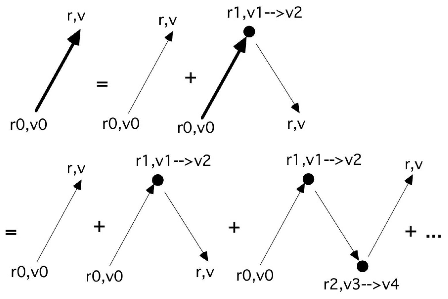
Now, we can introduce here a notation well known in quantum field theory [60] where G, the Green function of the equation, is the exact propagator, while we use g to represent the Green function where the positive part of the collision operator J is removed, so that particles just propagate according to the convective operator while they “decay” and disappear according to the exponential . The result is the expansion:
The expression above is quite complex, and its subsequent orders are increasingly cumbersome, but it can be conveniently summarized by diagrams as shown in Figure 1.
In the figure, once again using a notation borrowed from quantum field theory [61], an arrow represents a Green function, a dot represents the effect of integration and of the positive part of the collision operator J, a thick arrow represents the exact Green function G (i.e., the Green function of the full transport equation). Here, g, the thin arrow, represents not just collisionless particle propagation, but includes exponential decay. This is essential for the full G, the thick arrow, to conserve the normalization of f. If the null-collision method is used, the operator represented by the dot contains a term not affecting f and a term with , .
The factor , which precedes the second term in Equation (7) takes into account the fact that a collision at followed by a collision at is equivalent to the same collisions in opposite order. The term of n-th order will therefore be preceded by a factor . If the perturbation expansion is written using the null collision method, then a factor of the type will appear in front of each term in the expansion [57,59]; the details of the derivation are sketched in the next section. These factors constitute a Poisson distribution, which can be generated using the formula for collision times (2). In this way, the formula normally introduced on an empirical basis finds a mathematical motivation.
These diagrams show that the null-collision MC method is in fact directly related to a specific form of the transport equation [55]. Indeed, it is possible to formally state that, given a set of MC simulations of a given case study, the subset that includes exactly n-collisions corresponds to a stochastic calculation of the term of n-th order in a perturbation expansion of the solution of the equation transport.
Sometimes, one can be misled by the fact that the MC method introduces statistical fluctuations of the quantities then felt in the transport equation, such as the kinetic distribution of velocities. This seems to show that it has a higher element of describing reality than these equations. In reality the statistical fluctuations of the MC method are not physical and simply have to be reduced as much as possible by accumulation of events, leading to statistical convergence towards the exact solution. The method always converges to it for an infinite number of events, when the solved equation is linear. We take advantage of this aspect to underline again something that is also essential in the other sections of this review, namely the fact that swarm problems are generally described by linear equations, given that the particles of the swarm are diluted to the point of not interacting. This is a basic requirement to apply the concept of the Green function.
These considerations allow us to place the MC method, normally considered a technical tool in the field of plasma simulation, in the broader context of methods for theoretical physics. This is a very appropriate position given that it is formally capable of solving the Boltzmann transport equation, and not only as a numerical experiment, from an analogical point of view, as the terminology often used in publications seems to suggest [2,6].
This physical-mathematical aspect of the method can easily go into the background, precisely because of what is perhaps its greatest advantage; in its most basic implementations it can be developed precisely having in mind a direct image of the physics of the transport process.
3. The Monte Carlo Flux Method
3.1. Principle
In the previous section, we noted that the traditional MC method corresponds in any case to a formal calculation, i.e., the calculation of the Green functions, or electron propagators. These functions are generalized functions (i.e., Dirac delta functions), with a diffuse component which becomes the majority as time increases, precisely due to collisions [59]. The computed Green functions in each case depend on continuously varying arguments, which represent initial and final position and velocity components.
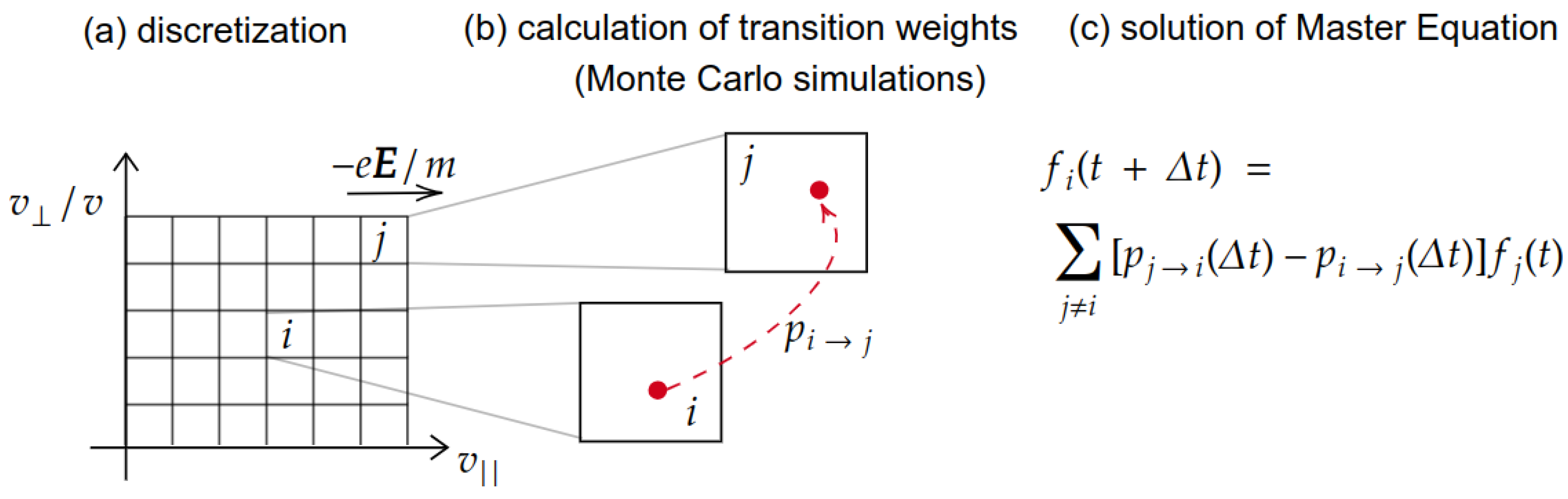
Since the beginning of the 1990s, modifications of the method have been experimented, in which instead of calculating propagators at the level of description of the electrons for the entire simulated time, the formalism of Markov processes has been employed to separate the diffusion time scale from the collision scale [62]. Among these, the Monte Carlo Flux method (MCF) stands out in particular, which is a hybrid method between the deterministic method of the propagators and the stochastic MC method [41]. The fundamental idea of this method is the separation between diffusion and collisional time scales. In fact, due to the small mass of the electron compared with that of atoms and molecules, in some very common regimes, hundreds of collisions are needed to observe a significant average dispersion of the initial kinetic energy. It is therefore convenient to describe the diffusive phase by means of averaged quantities obtained previously from calculations describing the effect of the collisions on the single electrons. To make this calculation practical, it is advisable to carry out a coarse-grained preliminary operation by introducing a lattice of suitable geometry into the configuration space. Once this is done, diffusive kinetics over long times can be described using the Master Equation or Kolmogorov equation [62,63] (i.e., the balance of probability over time).
The schematics of MCF is shown in Figure 2, where the three main steps of the numerical methods are highlighted (in order from left to right). The transition frequencies , which appear as coefficients depending on two indices and on time in the equation are precisely the quantities which can be calculated by means of a collection of traditional MC simulations [41]. In each of these collections of simulations, electrons are uniformly distributed within a cell of the lattice in the configuration space and a simulation of the duration corresponding to a few collisions is therefore performed. At the end of the simulation, the electrons found in each of the cells estimate the transition frequency between the initial cell and the final cell. Running this collection of preliminary simulations can take significant time, as it is necessary to break down for each individual cell. However, the Markov matrix that is calculated in this way can be used as a Green function in coarse-grained space and for a fixed time difference, so that it is possible to perform different simulations, for different times as long as they are multiples of , and for several initial distributions, all without the need to run the preliminary MC simulations again. Alternatively, the stationary distribution can be calculated by looking for the stationary vector with respect to the matrix. All of these calculations are completely deterministic and pretty fast.
3.2. Mathematical Derivation of Monte Carlo Flux
In this subsection, the MCF method is derived starting from a continuous generalization and proceeding with its discretized form, obtained under the multigroup approximation [64]. This subsection is based on Chapter 3 of the Ph.D. thesis of one of the authors [65].
The system under consideration is assumed to be homogeneous, such that spatial terms in Equation (1) are neglected. A possible technique for the solution of the homogeneous, linear EBE is based on the path-integral formulation, as described by Rees [66]. In Ref. [66], the rigorous path-integral theory has been initially developed for transport studies in semiconductors. The same theory has been extended by Kumar [67] and Longo [55] for the motion of charged particles in a gas in the presence of an external field. The use of this formulation has a two-fold advantage, that is; (i) the null-collision technique [54] is directly derived from the transport problem and (ii) the solution of Equation (1) is obtained by iterative applications of a continuous generalization of a Markov operator on the initial EVDF. In particular, from Equations (5) and (6), it is possible to verify that Equation (1) can be rewritten as
where
and is the maximum collision frequency defined such that for all values of the electron speed v. Note that the first term on the right-hand-side of Equation (9) represents the gain of electrons having velocity at time t due to collisions with the background gas, and the term represents “null-collision” events per unit time that leave the EVDF unchanged. The definition of is also widely used in MC simulations, since it is at the basis of the null-collision technique introduced by Skullerud [54]. For stationary conditions the solution of Equation (8) is
The method for evaluating the right-hand-side of Equation (10) is based on the following iterative technique [66]. First, an intermediate function for the -th iteration is generated from , as
Second, the distribution is obtained from as
The advantage of this method is that the n-th iterate is equivalent to the distribution obtained after a time interval . Furthermore, the stationary EVDF can be obtained in the limit .
As described by Nanbu [68], the same iterative approach can be applied when the temporal evolution of the EVDF is sought after. In particular, for sufficiently high values of , let be the time step for EVDF evolution. Then, at first order in , the EVDF can be expressed as
or equivalently
If is sufficiently low, an iterative solution of Equation (8) also describes the temporal evolution of the EVDF, starting from an initial distribution , at time .
To summarize, it is useful to represent the aforementioned equations in a schematic form. In particular, the integration on the right-hand-side of Equation (11) can be represented as the action of an operator on and that on the right-hand-side of Equation (12) by the action of an operator on . A complete iteration is therefore described by the action of the combined operator on . Moreover, the time evolution of an initial function after a time interval is determined by . Different numerical techniques can be employed for calculations of the aforementioned operator. In the MCF method, a grid is defined for calculations of transition weights for the electron motion between velocity space cells. In this discretized form, is also termed as the transport matrix (or Markov matrix). The following subsections are devoted to the description of this discretization and the numerical procedure that is applied for calculations of .
3.3. Discretization of the Electron Velocity Distribution Function
We describe here the numerical method that is used to implement the MCF. A more detailed comparison of MCF against other methods, such as conventional MC, two-term Boltzmann solver, and multi-term Boltzmann solver, is described in Refs. [41,69,70]. Furthermore, the method has been recently coupled with detailed plasma chemistry models in Refs. [71,72,73,74].
In this subsection, a uniform external electric field is considered, such that . Hence the electron velocity can be represented in polar coordinates , where is the electron kinetic energy (i.e., ), is the angle between and the z-direction, and is the azimuthal angle around the z-axis. Under the assumption of isotropic scattering around the z-axis, the velocity space can be described by two variables only , instead of three. Moreover, under this assumption, the EVDF is uniform in (i.e., ). Hence the velocity space is partitioned into cells , with the index for the energy component and the index for the angular component. The calculation range is assumed as and , where is chosen such that we can neglect electron diffusive fluxes to energies higher than . In this way, the energy and angular bin sizes are defined as and .
Under these assumptions, the EVDF can be represented in its discretized form as a column vector of size as
where each element of the vector has size and represents the total number of particles having energies between 0 and and , with . In particular, the j-th component () is written as
where is the total number of electrons in the cell and it is computed as
where is the total number of particles in the MC simulation and
In other words, after discretization of the energy and angular components, each simulated particle contributes to the EVDF as a Kronecker delta function [15]. From the EVDF, the l-th order Legendre polynomial coefficients can be calculated as
where is a normalization factor that depends on the total electron population , such that
is the transpose vector for the EVDF computed at , thus having size , and is a column vector of size written as
with the l-th order Legendre polynomial calculated at . Note that the Electron Energy Distribution Function (EEDF) comes from Equation (20) as the zero-th order (isotropic) component () of the EVDF expansion. Hence can be calculated with the following simplified expression:
meaning that the EEDF can be retrieved directly from binning in energy of the total number of simulated particles. In the following, the basic idea underlying MCF simulations is covered, that is the calculation of the temporal evolution of the EVDF, given an initial distribution at time .
3.4. Calculation of the Transport Matrix
In the MCF method, the temporal evolution of the EVDF is obtained by a matrix-vector operation, given an initial distribution function at the time . The EVDF at time is computed as [41]
where is the transport matrix of size . Note that the matrix is a discrete version of the continuous operator defined in Section 3.2.
More generally, if the reduced electric field and the gas composition are fixed for any , the transport matrix remains unchanged and the EVDF can be found with an iterative procedure as
with n the iteration number, and the time-step associated with the n-th iteration. An important consequence of Equation (25) is that the evolution of the system after is determined only by the state of the system at a time t and it is not affected by the previous history. This is known as Markov property and allows one to rewrite the linear EBE (Equation (1)) as a simple Markov chain consisting of the system of linear equations in (25). This property is typically satisfied if , that is, should be much longer than the time interval between two successive collisions , but also shorter than the time for the distribution function to reach steady-state. In particular, collisions are essential for the randomization of the particle velocities and trajectories. Through this randomization, electron history is erased and the evolution of the system depends only on the current state, not on past states. Hence, as shown in Refs. [69,70], the choice of an appropriate is fundamental to ensure the applicability of Equation (25).
The form of the transport matrix is
where are sub-matrices of size . The total number of sub-matrices in Equation (26) is determined by the angular discretization. For example, if J cells are defined for the angular component, then all the possible combinations are included in . Each sub-matrix is written as:
where is the transition weight for electrons moving from cell to within the time interval . In the MCF method, short MC simulations are performed for calculations of transition weights between all velocity space cells. Hence, transition weights in Equation (27) are calculated as
where is the total number of electrons moving from cell to within the time interval and is the total number of electrons in the initial cell at time . Note that the time interval depends on physical parameters such as the electric field E and the gas number density N. Empirically, it becomes shorter at higher E and N, as the electron collision frequency increases. The choice of an optimal is important for an optimization of the CPU time in MC simulations, as well as for accurate calculations of transition weights [69].
3.5. Advantages and Disadvantages
- Since the MCF is used to calculate the transition frequency and not directly the kinetic distribution, the MCF results have uniform statistical fluctuations for all the regions of the distribution, in particular also the tail, which instead may be statistically inaccessible to the traditional method given the low number of electrons described;
- The matrix-based approach does not require a series expansion of the EVDF and it is easier to implement than a multi-term Boltzmann solver. In perspective, the MCF method can be combined with efficient algorithms for matrix operations and GPU acceleration;
- As a difference with respect to other variance reduction techniques, mainly based on variable mathematical weights for the simulated particles, the MCF method addresses the fundamental problem of the very large ratio, amounting to several orders of magnitude, between the relaxation time of the distribution and the inter-collision time. Hence, the stochastic part of MC simulations is limited to a small time interval, which is typically orders of magnitude lower than the steady-state time for the electron energy distribution function (EEDF).
However, in spite of the advantages of this method in terms of both computational cost and accuracy with respect to a conventional MC method, a number of disadvantages of MCF should be considered when choosing an appropriate computational method for plasma applications. For example:
- The increasing size of the transport matrix lengthens the computational time and this is also a limit for practical use of the MCF method. This is a problem, for example, for an extension to the configuration space, since additional calculations of transition weights of electrons moving between different cells in the spatial coordinates are needed. Nevertheless, matrices in this case are largely sparse. Hence, the use of efficient algorithms for sparse matrix calculations could help to reduce the large memory that is required;
- The method presented here can only deal with calculations of flux transport parameters. However, bulk parameters are needed when comparing results of calculated electron transport coefficient with swarm measurements, especially at high E/N [75]. An extension of the MCF method to the configuration space will provide calculations of the aforementioned parameters as well;
- The transport matrix includes the effect of both field and collisional events. This has practical limitations for calculations of transition weights in the presence of a time-varying electric field evolving in timescales comparable with the energy relaxation time. In fact, this limits the applicability of MCF to DC and high frequency fields, and makes MCF not suitable for studies of RF or pulsed discharges.
Some of the limitations of the MCF method can be overcome by the Propagator method that is described in the following Section, where the field acceleration is separated from the collision part by defining different propagator matrices similar to the transport matrices used in MCF. This makes the Propagator method also applicable to AC electric fields. However, the Propagator method is limited to low such that the electron outflow from a cell does not exceed the total number of electrons in that cell [76]. Furthermore, it is important to highlight that, as a difference with respect to the Propagator method and the Convection scheme [77], the MCF uses MC simulations for calculations of transition weights between velocity space cells. The use of MC simulations is advantageous for its simpler implementation with respect to efficient convective schemes, but it is computationally expensive for large domain simulations.
4. Propagator Method
4.1. Principle
Propagator method (PM) is a numerical scheme to calculate the EVDF (or EEDF) on the basis of the EBE. The PM shares many common concepts with the MCF method. The PM calculation is performed with cells defined by partitioning of phase space , velocity space, and real space into small sections in which the electrons distribute. The number of electrons belonging to a cell is stored in an element of a matrix or an array corresponding to the cell. The probability of inter-cellular electron transition from a source cell to destination cells in a short time step is again represented by a Green function. The transition may be caused by the velocity change under electric and magnetic fields and scattering at collisions with gas molecules. The PM does not use random numbers, and its calculation is completely deterministic. The stochastic processes are considered on the bases of their expected values. Temporal development of the EVDF is observed by applying the acceleration and collision propagators to the EVDF every . The PM has a flexibility in treatment of the propagators as seen in practical examples introduced in the following sections. The step-by-step time development of the EVDF can be modified in some specific models customized to derive only equilibrium solutions, and the PM can deal with some simple boundary conditions such as electron reflection and secondary electron emission at electrode surfaces.
There are various cell configurations and experimental models for the PM calculations depending on the target properties of electron swarms. Let us overview the efforts of calculations that have been performed using the PM.
4.2. Classification of Cell Configurations and Expressions of Electron Motion
We may classify the types of the PM configurations on the basis of the partitioning of velocity space for cells and the expressions of the electron motion in the quantification of the intercellular electron transition.
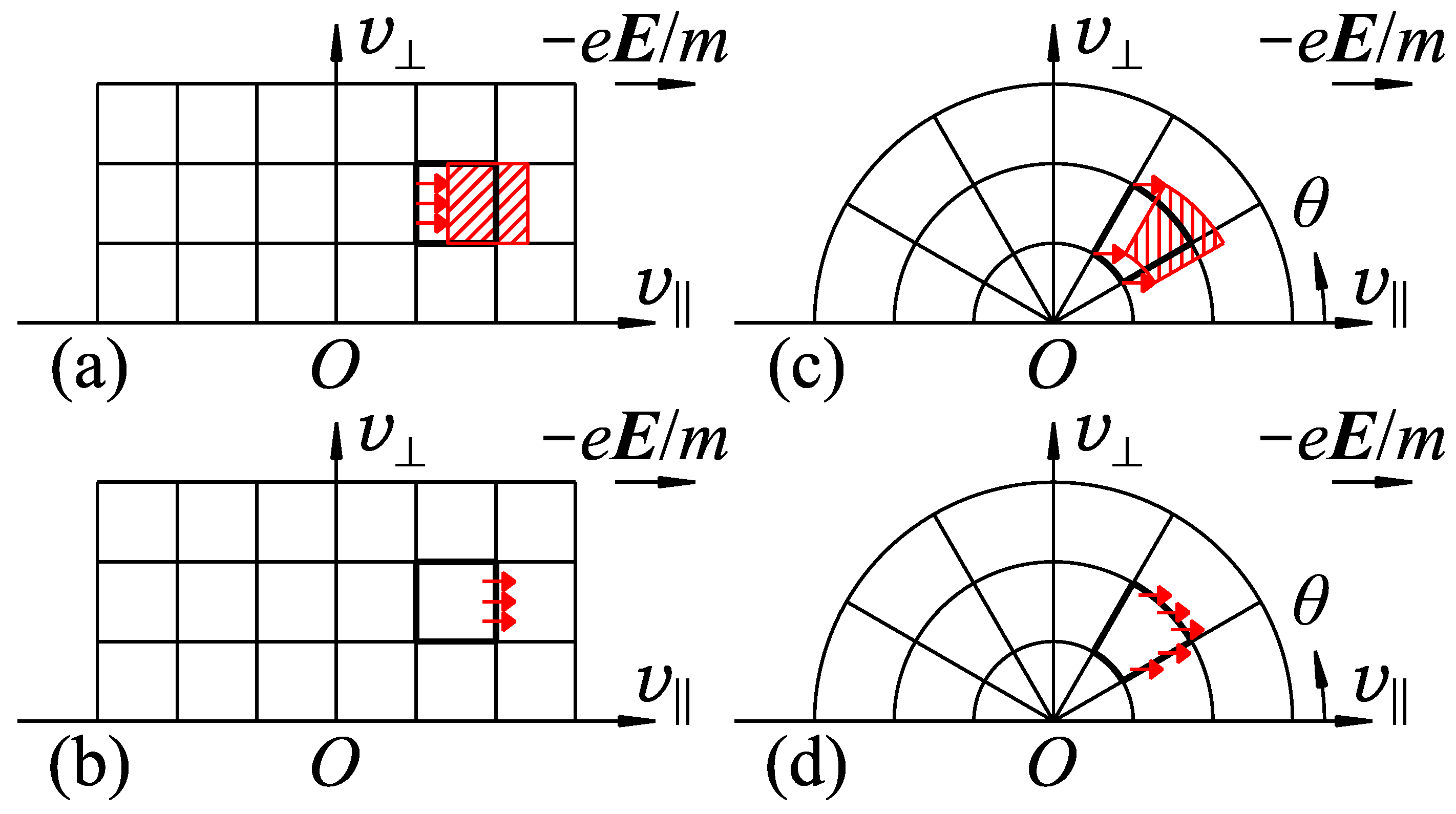
For the former point, the cells can be defined, for example, for every , , and in Cartesian coordinate system (Figure 3a,b), or for every , , and in polar coordinate system (Figure 3c,d), where , , and . In addition, division for every instead of is also possible. They are referred to as Cartesian-v, polar-v, and polar- configurations of the cells for velocity space in the following sections.
For the latter point, Lagrangian and Eulerian expressions are considered for the treatment of electron motion in the acceleration or flight. In the Lagrangian expression, the source and destination cells are related by ballistic motion of electrons starting from the source cell (Figure 3a,c), For example, if the electrons in a source cell undergo a collective free flight for , they would appear as if they are a moving cell, which is called a Lagrangian cell. The destination cells are chosen as those located at the position where the Lagrangian cell reaches after , and the ratio of the electron redistribution that the destination cell accepts from the source cell is calculated as the ratio of the area overlapping between the Lagrangian cell and each destination cell. On the other hand, in the Eulerian expression, source and destination cells are assumed to contact each other and to share the cell boundary between them. The number of electrons moving out of the source cell to the destination cell, , is evaluated by integrating the electron flux passing through the cell boundary during (Figure 3b,d). Its amount is evaluated as , where [] is the area of the cell boundary projected to a plane perpendicular to , is the number of electron in the cell, [] is the volume of the cell, and [] is the electron acceleration. must be short enough to avoid for all cells.
4.3. Collision Propagator
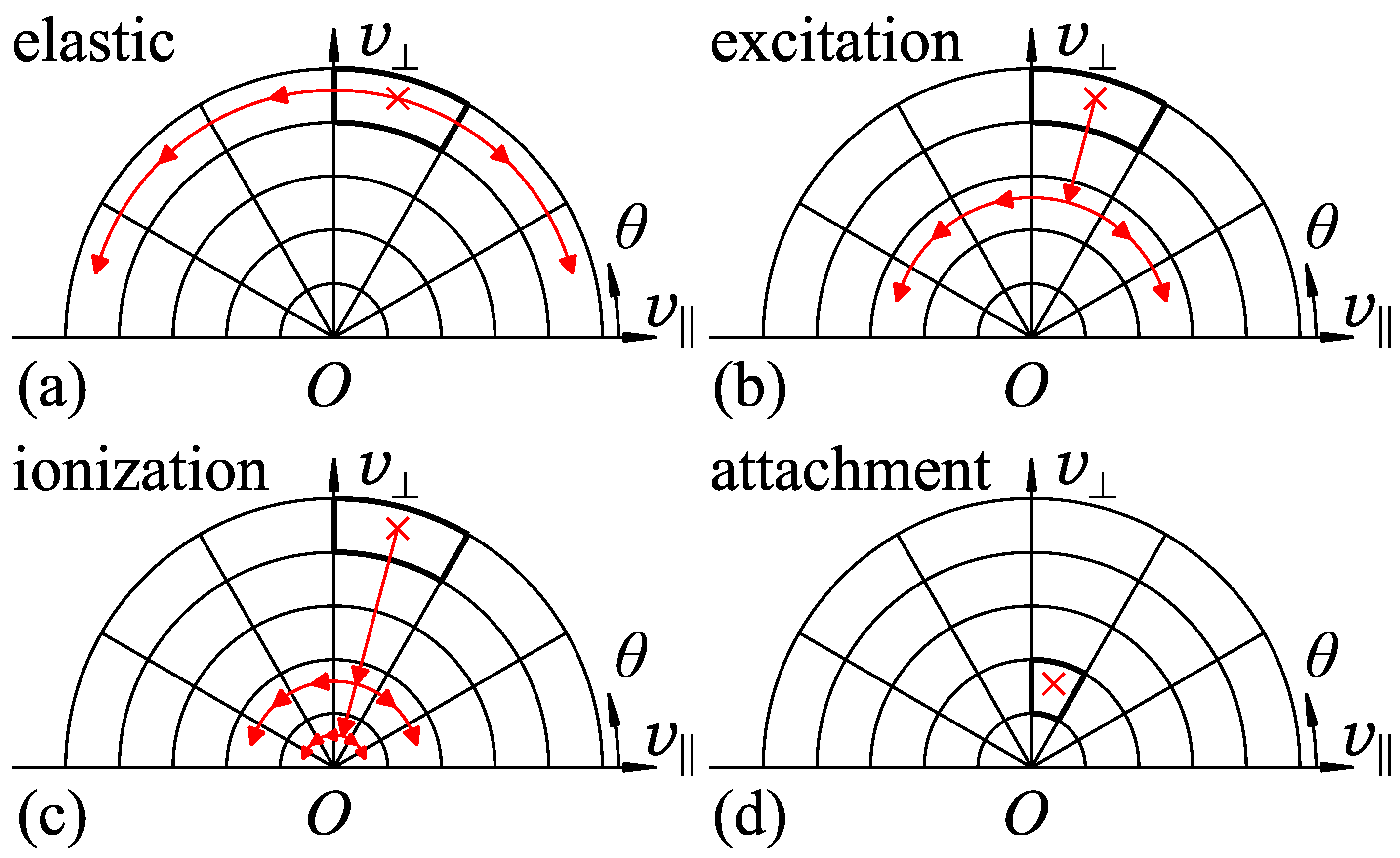
The collision propagator represents the change of electron velocity due to collision and scattering. The collisions are categorized into mainly four types. In the simplest case, the following processes are assumed for the electrons undergoing collision at an energy .
- Elastic collision
- The electrons are scattered isotropically without loss of energy. They are redistributed to the destination cells having the same energy in proportion to the solid angle of the destination cell subtended at the origin of velocity space (Figure 4a).
- Excitation collision
- The electrons lose excitation energy and are redistributed to the lower-energy cells of (Figure 4b).
- Ionization collision
- The electrons lose ionization energy and the residual energy is shared by the primary and secondary electrons. The electrons, which are doubled, are redistributed to the lower-energy cells of with relevantly given ratios under the law of energy conservation (Figure 4c).
- Electron attachment
- The electrons captured by gas molecules disappear from velocity space (Figure 4d).
The number of electrons undergoing collisions of the kth kind in a cell during , , is evaluated as , where N is the gas molecule number density, and is the electron collision cross section of the kth kind of collisional process as a function of the electron speed v. The portions are subtracted from of the source cell, and distributed to the destination cells corresponding to the electron velocity after scattering. must be short enough so that the probability of multiple collisions during can be neglected, and to satisfy .
Figure 4.
Treatment of electron collisions and scattering: (a) elastic collision, electron redistribution to the cells of ; (b) excitation collision, electron redistribution to the lower-energy cells of ; (c) ionization collision, electron doubling and redistribution to the lower-energy cells of ; and (d) electron attachment, electron disappearance from velocity space. The cells with thick boundaries and red crosses are the source cells, from which electrons flow out. is the energy of the incident electron. and are the excitation and ionization energies, respectively.

4.4. Models of Velocity-Space under Uniform Electric Fields
The PM calculation for the temporal development of the EVDF of an electron swarm under a uniform electric field is the simplest self-consistent model. It assumes an electron swarm in boundary-free real space and the position of each electron is ignored. The field may be dc, ac (typically rf: radio frequency), or even impulse fields.
The EBE for this model is written as
The spatial electron distribution has already been integrated and its profile is not investigated here.
The EVDF in this model can be assumed to be in a rotational symmetry for the azimuthal direction around the -axis. Thus, the EVDF can be represented as a two-variable distribution as or . Here, and are components of parallel and perpendicular to the direction of , respectively, and .
Some of the earliest PM efforts to obtain adopted the Cartesian-v configuration with and under dc [78,79] and rf [80] fields. Such a cell configuration simplifies the calculation of the electron acceleration because it is a parallel shift to the direction in velocity space. Each cell has a boundary in contact with its downstream neighbor, and the boundary is normal to . The probability of electron transition from a cell can be calculated easily in both Eulerian and Lagrangian manners. The Cartesian-v configuration has also been adopted in calculation of extended to a parallel-plane electrodes model including one-dimensional real space z [81,82,83]. In the one-dimensional real-space model, there are different treatments for simultaneous changes of and z in an electron flight, which is explained in the next subsection.
On the other hand, polar-v or polar- configuration with or , and or makes the redistribution of electrons after collisions simple when isotropic electron scattering is assumed. The ratio of the scattered electrons that a destination cell receives is proportional to the solid angle of the cell subtended at the origin of velocity space in case of isotropic scattering, and the sold angle of a cell is given from sin. Such a polar- configuration has been adopted not only for in velocity space in pulsed Townsend (PT) mode [76,84] but also for the steady-state Townsend (SST) mode [85,86,87], for the time-of-flight (TOF) mode [76,88,89], and rf [90] and impulse [91] fields as mentioned afterward.
4.5. Models of Configuration Space between Parallel-Plane Electrodes
The EVDF in one-dimensional configuration space between parallel-plane electrodes is a function of three-variable that are or . In the point of required memory capacity for practical calculations, it is beneficial that the range of z is finite between the electrodes. The computational array for the cells becomes three-dimensional, and cells are prepared for every , , and [81,82,83], or for every , , and [85]. The same collision propagator as used in the velocity-space model can be applied to this mode because the scattering changes only of electrons and their positions are unchanged at that moment. The acceleration propagator involves the spatial displacement because and z change at the same time in electron free flight under an electric field.
In some early PM efforts using cells defined for every , , and [81,82,83], the destination cells were chosen under a concept of Lagrangian cell. The choice of destination cells and evaluation of the electron redistribution ratios for them are easy in the Cartesian-v configuration because the geometrical shape of cells is simple. This treatment also allows flexible change of not only for DC but also for RF [82,83] or position-dependent [81,82].
On the other hand, treatment of electron displacement in an Eulerian approach was also attempted [85], adopting restrictions for the cell configuration and the intercellular electron motion. The cells are defined for every , , and to satisfy . The number of electrons flowing out of a source cell is evaluated by integrating the electron flux passing through the downstream cell boundary in velocity space. The changes of and z are strictly bound under the law of conservation of energy. A demonstration was made under a SST condition by superposing a temporal development of an isolated electron swarm starting from the cathode with an initial energy until almost all electrons are absorbed by the anode. Under the restrictions to guarantee the energy conservation, position-dependent profiles of spatial relaxation processes of mean electron energy and drift velocity agreed with results of a MC simulation. In particular, the rising position of ionization coefficient was successfully reproduced at , where is the ionization threshold, by suppressing the numerical diffusion which may occur among the destination cells in the Lagrangian approach.
The boundary condition at the electrodes is also a point of discussion. The simplest model assumes perfect absorption, where the electrons reaching the electrodes disappear. Elastic or inelastic reflection at the electrodes can be considered by relevantly choosing after reaching either of the electrodes. The effect of secondary electron emission [82] can be considered as a practical condition as well by supplying new electrons to the cells near the electrode on which primary electrons impinge.
4.6. Models of Boundary-Free Real Space in Steady-State Townsend Condition
When SST condition is assumed for one-dimensional electron flow in z direction under uniform electric field , partitioning of the z position can be omitted [86] in the PM calculation for the EVDF by utilizing the assumptions that the normalized EVDF is identical irrespective of z and that the electron number density varies exponentially with z as , where is the effective ionization coefficient. The EVDF is available from the PM calculation performed with only cells for velocity space. Such a technique allows one to reduce the required memory capacity.
If the EVDF in a slab is in equilibrium, the electron flow at is times as large as that at z. The PM calculation considers only in the slab. A polar- configuration was adopted and was set to be to take account of the conservation of energy [86]. Electrons in the slab may flow out of the slab, but other electrons flow into the slab from the opposite side to keep the electron population in the slab unchanged. The outflow can be evaluated directly from the EVDF in the slab in the same way as done between parallel-plane electrodes. The inflow is evaluated using the assumption of exponential spatial growth. Let and be the numbers of electrons flowing out of the slab forward () at and backward () at , respectively, and and be those flowing into the slab forward at and backward at , respectively, during a time step . Their relations are
The value of is unknown at this moment. However, with and respectively being the electron increase and decrease due to ionization and attachment during , the value of is obtained from a quadratic equation derived from the electron conservation in the slab. They satisfy
This treatment is equivalent to the assumption and in two-term approximation of the EBE analysis for the SST condition [92]. is obtained from
The positive sign is taken in usual SST condition so that when . By a relaxation of the EVDF starting from initial EVDF and , the EVDF in equilibrium under the SST condition is obtained.
Another solution of the quadratic formula corresponding to the negative sign is understood to represent properties of electrons in backward diffusion. In this case, no longer represents the exponential growth of by ionization, but it represents the decay of toward the direction in the upstream region from the electron source [87,93]. A PM calculation with such [87] demonstrated that the EVDF obtained in the upstream region represents the properties of the missing electrons [94] producing the decay of in front of the absorbing anode [81,85].
4.7. Models of Boundary-Free Real-Space Time-of-Flight Condition
The spatial electron distribution can be composed by superposing the kth-order Hermite functions up to a sufficient order n [88]:
where is the kth-order Hermite polynomial derived sequentially from by a relation , is the weight of the kth-order Hermite function, is the center of mass of the whole electron swarm, is the standard deviation of electron position z, and is the dimension-less z position. satisfy an orthogonality , where is the Kronecker delta. The Hermite functions are suitable to expand or compose Gaussian-like distributions having boundary condition , and it is thought that of electron swarms eventually tends to a Gaussian. Values of are determined by the spatial moments of the electron swarm up to the kth order, as shown later.
Let be the kth-order spatial moment distribution function with respect to the z direction, and it is defined as
A series of moment equations in a hierarchy are derived from the EBE by integrating each term with weight over z [76,88,89], and can be calculated without the partitioning of z:
Here, is identical to representing the electron number density at . gives the center of mass of the electrons having as , and the center of mass of the whole electron swarm is given as . The temporal variation of is the center-of-mass drift velocity of the electron swarm [76,88,89,95,96]. gives the variance of the electron swarm as . Its temporal variation gives the longitudinal diffusion coefficient as [76,89,95,96].
For the moment calculation up to the nth order, sets of cells are prepared, and initial values of () are stored in the cells. Their temporal variations for are calculated by applying the collision and acceleration propagators to . The propagators are common for irrespective of k. In addition, amounts of the kth-order moments evaluated by the drift term are added to to obtain . The instantaneous amount of the kth order moment of the whole electron swarm is given as . , which are values in laboratory system, are converted to the values in center-of-mass system around as . From these quantities we can obtain higher-order (nth-order, ) diffusion coefficients as well [89]; e.g., . are further converted to to the dimension-less value reduced by as . Some are given as
The same technique to compose spatial electron distribution has been applied not only to the longitudinal direction [89] but also to the transverse direction [97]. The higher-order transverse diffusion coefficients are also available from the simultaneous moment equations up to the nth order with respect to the direction perpendicular to the field [97].
4.8. Models of Velocity Space and Real Space under Uniform Electric and Magnetic Fields
The PM has been applied to calculation of the EVDF in equilibrium under dc crossed electric and magnetic fields, fields, assuming as () and () [98]. The EVDF is no longer axi-symmetric under the fields, thus it is required to have three variables to represent the EVDF. A polar- configuration modified for three-variable velocity space was chosen in the practical calculation for convenience in the treatment of isotropic scattering after collisions [98]. The memory array for the EVDF becomes three-dimensional as the cells were prepared for every , , and , where , is the electron speed associated with eV, , , and . A cell may have at most six boundaries facing to the , , and directions. The EBE for the EVDF in velocity space becomes
The treatment for the collision operator is unchanged even for the EVDF in the fields. On the other hand, the acceleration is velocity-dependent and electron motion in velocity space is rotational around an axis . This rotation axis is parallel to the axis but off-centered (off-origin). This creates a complexity in the preparation of the acceleration propagator. The probability of the intercellular electron transition is calculated in the Eulerian approach common with that applied to two-variable velocity space, i.e., by integration of the outflow flux at the downstream cell boundary. However, the cell boundaries facing to the ‘downstream’ depends on the acceleration direction determined by . Further more, the acceleration direction may change even in a cell boundary. The acceleration propagator to deal with the rotational electron flow was prepared choosing the downstream cell boundaries carefully, and the order of application of the acceleration propagator to the cells are also arranged for fast convergence of the EVDF.
In an example of computation of the EVDF under fields with cells for in double precision (8 bytes per cell) [98], the required memory capacity was roughly several GiB. In addition to the array to store the numbers of electrons in the cells, those for associated cell properties such as cell volume and areas of the six cell boundaries are also needed. However, the memory capacity required for this model is within an available range for recent workstations.
The EBE under the fields can also be extended to the spatial moment equations under the fields with respect to the x, and y, and z directions [99] in the same approach as Equation (39) performed in the boundary-free one-dimensional TOF model. The center-of-mass drift velocity vector and the direction-dependent diffusion coefficients , , and were calculated by the PM for the simultaneous spatial moment equations up to the second order. Seven sets of cells were used to store the zeroth-, first-, and second-order moments with respect to the x, y, and z directions, , , , , , , and , where is common for the three directions. The collision and acceleration propagators are unchanged. Temporal development of the moments can be calculated by applying the propagators iteratively. On the other hand, in case only the equilibrium values of , , , , , and are needed, the relaxation of each moment can be achieved stepwise from the zeroth order to the second independently for x, y, and z, because higher-order moments depend on only the lower-order ones defined for the same direction via the drift term. This feature allows us to save the computational load for the relaxation process and the required memory capacity.
4.9. Challenges in Computational Techniques
It is an advantageous feature that the PM can follow the temporal development of the EVDF. On the other hand, we often need only the EVDF solution in drift equilibrium. In conventional PM calculations, the equilibrium EVDF is obtained after physical relaxation of the EVDF under the electron acceleration by the external fields and scattering by gas molecules proceeding step by step every . This guarantees the continuity of the number of electrons. When the difference between the normalized EVDFs derived from and is negligibly small, we may regard the EVDF as the converged solution. The normalized equilibrium EVDF satisfies the EBE, which is a balance equation under . The relaxation process of the EVDF can be accelerated by a scheme based on the Gauss–Seidel method [76]. In contrast to that, is kept unchanged until is obtained, and in case physical relaxation of the EVDF is observed, the Gauss–Seidel method renews part by part (i.e., cell by cell) on the basis of the local balance expressed by the EBE ignoring the entire electron conservation. It is expected here that renewed value of is closer to the equilibrium value than before renewal. Fast propagation of the renewal result over velocity space is promoted by arranging the sequence of renewal calculations to be from the upstream cells to the downstream cells in velocity space. This numerical relaxation process no longer has physical meaning. However, the number of iterations for convergence to the equilibrium solution can be reduced down to the order of magnitude of in a drastic case [76].
A challenge to a long-term relaxation process was demonstrated with a PM in a matrix form [42]. When the EVDF at a time t is represented in a vector form with the elements corresponding to the number of electrons in each cell similarly to Equations (15) and (16), can be obtained by applying a propagator represented in a matrix form as in the same way as Equation (24). Here, we may calculate powers of as , , , ⋯, by repeating the squaring operation for . After this preparation, we obtain . The relaxation time increases exponentially with n while computational elapse time increases linearly with n. The calculation for a slow relaxation of the EVDF in a ramp model gas [100] was demonstrated using cells defined with 1000 divisions for and 18 divisions for (thus, vector has elements), ps, and (, thus until ms) [42]. Convergence of mean electron energy and the EVDF were observed midway by . This approach enables us to observe a long-term relaxation in a logarithmic time scale, although it requires a large matrix size as .
Another recent improvement of the PM calculation is for calculations under low conditions and rf fields [90]. The polar- configuration has a tendency that the cells around the origin become more coarse than in the polar-v configuration. This feature is negligible at high values where the electron energy loss by inelastic collisions and the electron energy gain under high E are dominant in the formation of EVDF satisfying the energy balance. However, at low values, which appear not only under dc fields but also in rf fields as low periods, the coarseness of the low-energy cells leads to an overestimation of the acceleration of low-energy electrons and causes a less precision in some electron transport coefficients. This is because uniform electron distribution within a cell is used to be assumed in conventional PM calculations. It was demonstrated that the overestimation is suppressed by blending central and upwind differences with relevantly chosen weights.
Owing to the progress in both algorithm and computational facility, the PM is nowadays recognized as an available and possible self-consistent EVDF solver. With already established techniques, the PM can be used not only to solve the EVDF in typical observation models but also for preparation of look-up tables of a set of electron transport coefficients, mean electron energy , ionization coefficient , drift velocity W, and diffusion coefficient D under uniform dc , for the use in fluid simulations. Further enhancement of the calculation speed and memory capacity would allow us consideration for more practical effects of electron–molecule interactions, higher-order multi-dimensional cell configurations, and more complicated geometries of the plasma reactors. Some of the basic processes not dealt with sufficiently would be anisotropic scattering, super-elastic collisions, Coulomb collisions between electrons, etc. For the cell configuration, realization of PM calculation in dimensions higher than three would have to wait for more empowerment of the computers; e.g., self-consistent PM calculation in a cylindrical symmetry requires five-variable phase space as , which requires a tremendously huge memory capacity even with a coarse resolution for each variable. Nonetheless, for frequently assumed geometries such as one-dimensional real space between parallel-plane electrodes, the PM calculations done for three-variable phase space would withstand requirements on boundary conditions by its flexibility for linkage with, for example, Poisson’s equation and boundary conditions.
5. Summary and Conclusions
The methods that have been described in this review have in common that they describe the kinetics of electrons, subject to the effect of electric and magnetic fields and collisions with atoms and molecules in a low-temperature plasma, using a propagator-based description. Propagators are operators that shuffle the probability distribution of the electronic fluid in the phase space, moving it from one position to another in this generalized space: just as many mathematical objects of a certain importance can have a description apparently very different from another depending on the formal language on which the initial setting of the algorithm is based. This means that in some cases, such as in the writing of a so-called traditional MC program [32], the role of propagators may be much less evident at a superficial level. In some other cases [85], propagators enter not only into the settings of the algorithm but right from the beginning of the language that is used to describe it. A hybrid stochastic-deterministic approach, such as the MCF [41,69], which effectively uses the propagators twice, first as “micro-propagators” for calculations of transition weights, and then as Markov matrices to extend the simulation to the characteristic times of energy diffusion, is an even more particular case.
Emphasizing the common roots of these approaches and others that are comparable does not erase the fact that in the concrete study of a certain type of ionized gas rather than another a method in particular may be much superior to others. Elements that contribute to this choice are the relationships between the various characteristic times of the plasma, the type of collision processes, the dimensionality of the system, the presence and complexity of boundary conditions, and even practical requirements such as the reduction of requested memory, speed and computer time, the physical transparency of the method, and ease of code maintenance. However, the ability to understand the conceptual bases and common aspects from a mathematical point of view of the calculation methods available for the study of the electron kinetics of low-temperature plasmas can represent a very useful element of knowledge, both for researchers who have to decide the best strategy for the representation of a system and for instructors who teach these methods and express interest in them.
In all cases, the fundamental object in question is a time-dependent relationship between two states in phase space and which can be described physically as a function or as an operator acting on a function, and numerically as a matrix. Hence, its treatment requires tools from algebra and calculus. It is possible that the current approach to the simulation of plasma-based application systems, which is a modular approach, may hide the conceptual interest of these calculation tools: they constitute the most physical part of simulation programs and their connection with other areas of physics and mathematics are both aspects that can spark new interest in these tools. The mathematics of propagators allows us to solve the problem of the kinetics of plasma electrons with great efficiency, and this makes these instruments useful tools, because the kinetics of electrons in plasma cannot be neglected in reliably calculating chemical reaction rates and transport quantities.
Understanding the mathematical concept underlying a group of models is a stimulating exercise in itself and also has a heuristic value, because it produces future research questions:
- What is the most efficient presentation of the propagation concept depending on the conditions of plasma?
- How can the concept of propagation be extended to nonlinear systems such as those that emerge when collisions between charged particles or gas heating are taken into account?
- Can the mathematical grids that are employed at different times of the different approaches be replaced with spectral descriptions?
- Could propagators, which represent input–output relations, efficiently be computed using machine learning and artificial intelligence?
- Could the similarity between the propagators used in plasma and those used in other areas of physics help to develop faster or less memory-intensive computational methods?
More recent applications of low-temperature ionized gases from biology to space science to materials science will always produce new possibilities for numerical descriptions of electron transport that have new strengths—despite having their specific weaknesses. The authors hope that this review work can stimulate research activity that captures new insights and develops new languages.
Author Contributions
All authors have equally contributed to conceptualization. Conceptualization, L.V., H.S. and S.L.; writing—original draft preparation, L.V., H.S. and S.L.; writing—review and editing, L.V., H.S. and S.L. All authors have read and agreed to the published version of the manuscript.
Funding
L.V. acknowledges financial support by the Stanford Energy Postdoctoral Fellowship through contributions from the Precourt Institute for Energy, Bits & Watts Initiative, StorageX Initiative, and TomKat Center for Sustainable Energy. S.L. acknowledges funding under Mur-PNRR High Performance Computing, HPC_CN00000013.
Data Availability Statement
No new data were created or analyzed in this study. Data sharing is not applicable to this article.
Conflicts of Interest
The authors declare no conflict of interest.
References
- Villani, C. A review of mathematical topics in collisional kinetic theory. Handb. Math. Fluid Dyn. 2002, 1, 3–8. [Google Scholar]
- Cercignani, C. Mathematical Methods in Kinetic Theory; Springer: Berlin/Heidelberg, Germany, 1969; Volume 1. [Google Scholar]
- Desvillettes, L.; Mischler, S. About the splitting algorithm for Boltzmann and BGK equations. Math. Model. Methods Appl. Sci. 1996, 6, 1079–1102. [Google Scholar] [CrossRef]
- Balescu, R. Statistical Mechanics of Charged Particles; Wiley-Interscience: Hoboken, NJ, USA, 1963. [Google Scholar]
- Grad, H. On the kinetic theory of rarefied gases. Commun. Pure Appl. Math. 1949, 2, 331–407. [Google Scholar] [CrossRef]
- Duderstadt, J.J.; Martin, W.R. Transport Theory; John Wiley & Sons: Chichester, UK, 1979; 613p. [Google Scholar]
- Adamovich, I.; Agarwal, S.; Ahedo, E.; Alves, L.L.; Baalrud, S.; Babaeva, N.; Bogaerts, A.; Bourdon, A.; Bruggeman, P.; Canal, C.; et al. The 2022 Plasma Roadmap: Low temperature plasma science and technology. J. Phys. D Appl. Phys. 2022, 55, 373001. [Google Scholar] [CrossRef]
- Makabe, T. Velocity distribution of electrons in time-varying low-temperature plasmas: Progress in theoretical procedures over the past 70 years. Plasma Sources Sci. Technol. 2018, 27, 033001. [Google Scholar] [CrossRef]
- Kushner, M.J. Application of a particle simulation to modeling commutation in a linear thyratron. J. Appl. Phys. 1987, 61, 2784–2794. [Google Scholar] [CrossRef]
- Boyle, G.; Stokes, P.; Robson, R.; White, R. Boltzmann’s equation at 150: Traditional and modern solution techniques for charged particles in neutral gases. J. Chem. Phys. 2023, 159, 024306. [Google Scholar] [CrossRef] [PubMed]
- Braglia, G.L.; Romanò, L. Monte Carlo and Boltzmann two-term calculations of electron transport in CO2. Lett. Nuovo C. (1971–1985) 1984, 40, 513–518. [Google Scholar] [CrossRef]
- Braglia, G.L.; Wilhelm, J.; Winkler, E. Multi-term solutions of Boltzmann’s equation for electrons in the real gases Ar, CH4 and CO2. Lett. Nuovo C. (1971–1985) 1985, 44, 365–378. [Google Scholar] [CrossRef]
- Donko, Z.; Dyatko, N. First-principles particle simulation and Boltzmann equation analysis of negative differential conductivity and transient negative mobility effects in xenon. Eur. Phys. J. D 2016, 70, 135. [Google Scholar] [CrossRef]
- Hagelaar, G.; Donko, Z.; Dyatko, N. Modification of the Coulomb logarithm due to electron-neutral collisions. Phys. Rev. Lett. 2019, 123, 025004. [Google Scholar] [CrossRef] [PubMed]
- Yousfi, M.; Hennad, A.; Alkaa, A. Monte Carlo simulation of electron swarms at low reduced electric fields. Phys. Rev. E 1994, 49, 3264–3273. [Google Scholar] [CrossRef]
- Prigogine, I. Non-Equilibrium Statistical Mechanics; Courier Dover Publications: Mineola, NY, USA, 2017. [Google Scholar]
- Segur, P.; Yousfi, M.; Kadri, M.H.; Bordage, M.C. A survey of the numerical methods currently in use to describe the motion of an electron swarm in a weakly ionized gas. Transp. Theory Stat. Phys. 1986, 15, 705–757. [Google Scholar] [CrossRef]
- White, R.D.; Robson, R.E.; Dujko, S.; Nicoletopoulos, P.; Li, B. Recent advances in the application of Boltzmann equation and fluid equation methods to charged particle transport in non-equilibrium plasmas. J. Phys. D Appl. Phys. 2009, 42, 194001. [Google Scholar] [CrossRef]
- Rockwood, S.D. Elastic and inelastic cross sections for electron-Hg scattering from Hg transport data. Phys. Rev. A 1973, 8, 2348–2358. [Google Scholar] [CrossRef]
- Hagelaar, G.J.M.; Pitchford, L.C. Solving the Boltzmann equation to obtain electron transport coefficients and rate coefficients for fluid models. Plasma Sources Sci. Technol. 2005, 14, 722–733. [Google Scholar] [CrossRef]
- Tejero-del-Caz, A.; Guerra, V.; Gonçalves, D.; da Silva, M.L.; Marques, L.; Pinhão, N.; Pintassilgo, C.D.; Alves, L.L. The LisbOn KInetics Boltzmann solver. Plasma Sources Sci. Technol. 2019, 28, 043001. [Google Scholar] [CrossRef]
- Colonna, G.; D’Angola, A. Two-term Boltzmann Equation. In Plasma Modeling (Second Edition) Methods and Applications; IOP Publishing: Bristol, UK, 2022; pp. 1–2. [Google Scholar]
- Available online: https://github.com/IST-Lisbon/LOKI (accessed on 20 October 2020).
- Available online: http://www.bolsig.laplace.univ-tlse.fr/ (accessed on 1 February 2024).
- Dyatko, N.A.; Kochetov, I.V.; Napartovich, A.P.; Sukharev, A.G. EEDF: The Software Package for Calculations of the Electron Energy Distribution Function. Available online: https://fr.lxcat.net/download/EEDF (accessed on 1 February 2024).
- White, R.D.; Robson, R.E.; Schmidt, B.; Morrison, M.A. Is the classical two-term approximation of electron kinetic theory satisfactory for swarms and plasmas? J. Phys. D Appl. Phys. 2003, 36, 3125–3131. [Google Scholar] [CrossRef]
- Dujko, S.; White, R.D.; Petrović, Z.L.; Robson, R.E. A multi-term solution of the nonconservative Boltzmann equation for the analysis of temporal and spatial non-local effects in charged-particle swarms in electric and magnetic fields. Plasma Sources Sci. Technol. 2011, 20, 024013. [Google Scholar] [CrossRef]
- Loffhagen, D. Multi-term and non-local electron Boltzmann equation. In Plasma Modeling; IOP Publishing: Bristol, UK, 2016; pp. 2053–2563, 3–1–3–30. [Google Scholar] [CrossRef]
- Robson, R.; White, R.; Hildebrandt, M. Fundamentals of Charged Particle Transport in Gases and Condensed Matter; CRC Press: Boca Raton, FL, USA, 2017. [Google Scholar]
- Pitchford, L.C.; ONeil, S.V.; Rumble, J.R., Jr. Extended Boltzmann analysis of electron swarm experiments. Phys. Rev. A 1981, 23, 294–304. [Google Scholar] [CrossRef]
- Stephens, J. A multi-term Boltzmann equation benchmark of electron-argon cross-sections for use in low temperature plasma models. J. Phys. D Appl. Phys. 2018, 51, 125203. [Google Scholar] [CrossRef]
- Longo, S. Monte Carlo models of electron and ion transport in non-equilibrium plasmas. Plasma Sources Sci. Technol. 2000, 9, 468–476. [Google Scholar] [CrossRef]
- Boeuf, J.P.; Marode, E. A Monte Carlo analysis of an electron swarm in a nonuniform field: The cathode region of a glow discharge in helium. J. Phys. D Appl. Phys. 1982, 15, 2169–2187. [Google Scholar] [CrossRef]
- Penetrante, B.M.; Bardsley, J.N.; Pitchford, L.C. Monte Carlo and Boltzmann calculations of the density gradient expanded energy distribution functions of electron swarms in gases. J. Phys. Appl. Phys. 1985, 18, 1087–1100. [Google Scholar] [CrossRef]
- Spanier, J.; Gelbard, E.M. Monte Carlo Principles and Neutron Transport Problems; Dover Publications, Inc.: Mineola, NY, USA, 2008. [Google Scholar]
- Unpublished cross Sections Extracted. Available online: http://magboltz.web.cern.ch/magboltz/ (accessed on 1 February 2024).
- Biagi, S.F. Monte Carlo simulation of electron drift and diffusion in counting gases under the influence of electric and magnetic fields. Nucl. Instruments Methods Phys. Res. Sect. Accel. Spectrometers Detect. Assoc. Equip. 1999, 421, 234–240. [Google Scholar] [CrossRef]
- Rabie, M.; Franck, C.M. METHES: A Monte Carlo collision code for the simulation of electron transport in low temperature plasmas. Comput. Phys. Comm. 2016, 203, 268–277. [Google Scholar] [CrossRef]
- Dias, T.C.; Tejero-del Caz, A.; Alves, L.L.; Guerra, V. The LisbOn KInetics Monte Carlo solver. Comput. Phys. Comm. 2023, 282, 108554. [Google Scholar] [CrossRef]
- Taccogna, F. Monte Carlo Collision method for low temperature plasma simulation. J. Plasma Phys. 2015, 81, 305810102. [Google Scholar] [CrossRef]
- Schaefer, G.; Hui, P. The Monte Carlo flux method. J. Comput. Phys. 1990, 89, 1–30. [Google Scholar] [CrossRef]
- Sugawara, H.; Iwamoto, H. A technology demonstration of propagator matrix power method for calculation of electron velocity distribution functions in gas in long-term transient and succeeding equilibrium states under dc electric fields. Jpn. J. Appl. Phys. 2021, 60, 046001. [Google Scholar] [CrossRef]
- Gamba, I.M.; Rjasanow, S. Galerkin–Petrov approach for the Boltzmann equation. J. Comput. Phys. 2018, 366, 341–365. [Google Scholar] [CrossRef]
- Challis, L. The Green of Green functions. Phys. Today 2003, 56, 41–46. [Google Scholar] [CrossRef]
- Longo, S. Monte Carlo simulation of charged species kinetics in weakly ionized gases. Plasma Sources Sci. Technol. 2006, 15, S181–S188. [Google Scholar] [CrossRef]
- Pitchford, L.C.; Phelps, A.V. Comparative calculations of electron-swarm properties in N2 at moderate E/N values. Phys. Rev. A 1982, 25, 540–554. [Google Scholar] [CrossRef]
- Yousfi, M.; de Urquijo, J.; Juárez, A.; Basurto, E.; Hernández-Ávila, J.L. Electron Swarm Coefficients in CO2-N2 and CO2-O2 Mixtures. IEEE Trans. Plasma Sci. 2009, 37, 764–772. [Google Scholar] [CrossRef]
- Raspopović, Z.M.; Sakadžíc, S.; Bzenić, S.A.; Petrović, Z.L. Benchmark calculations for Monte Carlo simulations of electron transport. IEEE Trans. Plasma Sci. 1999, 27, 1241–1248. [Google Scholar] [CrossRef]
- Loffhagen, D.; Winkler, R.; Donkó, Z. Boltzmann equation and Monte Carlo analysis of the spatiotemporal electron relaxation in nonisothermal plasmas. Eur. Phys. J. Appl. Phys. 2002, 18, 189–200. [Google Scholar] [CrossRef]
- Andreev, S.; Bernatskiy, A.; Dyatko, N.; Kochetov, I.; Ochkin, V. Measurements and interpretation of EEDF in a discharge with a hollow cathode in helium: Effect of the measuring probe and the anode on the form of the distribution function. Plasma Sources Sci. Technol. 2022, 31, 105016. [Google Scholar] [CrossRef]
- Nolan, A.; Brennan, M.; Ness, K.; Wedding, A. A benchmark model for analysis of electron transport in non-conservative gases. J. Phys. D Appl. Phys. 1997, 30, 2865–2871. [Google Scholar] [CrossRef]
- Dyatko, N.; Napartovich, A. Electron swarm characteristics in Ar:NF3 mixtures under steady-state Townsend conditions. J. Phys. D Appl. Phys. 1999, 32, 3169–3178. [Google Scholar] [CrossRef]
- Tzeng, Y.; Kunhardt, E. Effect of energy partition in ionizing collisions on the electron-velocity distribution. Phys. Rev. A 1986, 34, 2148–2157. [Google Scholar] [CrossRef] [PubMed]
- Skullerud, H.R. The stochastic computer simulation of ion motion in a gas subjected to a constant electric field. J. Phys. D Appl. Phys. 1968, 1, 1567–1568. [Google Scholar] [CrossRef]
- Longo, S. Direct derivation of Skullerud’s Monte Carlo method for charged particle transport from the linear Boltzmann equation. Physica A 2002, 313, 389–396. [Google Scholar] [CrossRef]
- Ristivojevic, Z.; Petrović, Z.L. A Monte Carlo simulation of ion transport at finite temperatures. Plasma Sources Sci. Technol. 2012, 21, 035001. [Google Scholar] [CrossRef]
- Longo, S.; Diomede, P. Monte Carlo modeling of gas phase ion transport under thermal gradients and external fields. Eur. Phys. J. Appl. Phys. 2004, 26, 177–185. [Google Scholar] [CrossRef]
- Resibois, P.; Leener, M.D. Classical Kinetic Theory of Fluids; John Wiley and Sons: Hoboken, NJ, USA, 1977. [Google Scholar]
- Longo, S. The derivation of Particle Monte Carlo methods for plasma modeling from transport equations. arXiv 2008, arXiv:0805.3105. [Google Scholar]
- Berestetskii, V.B.; Lifshitz, E.M.; Pitaevskii, L.P. Quantum Electrodynamics; Butterworth-Heinemann: Oxford, UK, 1982; Volume 4. [Google Scholar]
- Mattuck, R.D. A Guide to Feynman Diagrams in the Many-Body Problem; The McGraw-Hill Book Company: New York, NY, USA, 1992. [Google Scholar]
- Van Kampen, N.G. Stochastic Processes in Physics and Chemistry; Elsevier: Amsterdam, The Netherlands, 1992; Volume 1. [Google Scholar]
- Gardiner, C.W. Handbook of Stochastic Methods; Springer: Berlin, Germany, 1985; Volume 3. [Google Scholar]
- Prinja, A.K.; Larsen, E.W. General principles of neutron transport. In Handbook of Nuclear Engineering; Springer: Boston, MA, USA, 2010; pp. 427–542. [Google Scholar]
- Vialetto, L. Modelling of Plasma for CO2 Conversion: Electron Kinetics, Chemistry and Transport; Technische Universiteit Eindhoven: Eindhoven, The Netherlands, 2021. [Google Scholar]
- Rees, H.D. The numerical analysis of semiclassical transport problems. J. Phys. C Solid State Phys. 1970, 3, 965–974. [Google Scholar] [CrossRef]
- Kumar, K. Short-time development of swarms-approach to hydrodynamic regime for charged particles in neutral gases. J. Phys. D Appl. Phys. 1981, 14, 2199–2208. [Google Scholar] [CrossRef]
- Nanbu, K. Direct simulation scheme derived from the Boltzmann equation. I. Monocomponent gases. J. Phys. Soc. Jpn. 1980, 49, 2042–2049. [Google Scholar] [CrossRef]
- Vialetto, L.; Longo, S.; Diomede, P. Benchmark calculations for electron velocity distribution function obtained with Monte Carlo Flux simulations. Plasma Sources Sci. Technol. 2019, 28, 115015. [Google Scholar] [CrossRef]
- Vialetto, L.; Viegas, P.; Longo, S.; Diomede, P. Benchmarking of Monte Carlo Flux simulations of electrons in CO2. Plasma Sources Sci. Technol. 2020, 29, 115006. [Google Scholar] [CrossRef]
- Viegas, P.; Vialetto, L.; Wolf, A.; Peeters, F.; Groen, P.; Righart, T.; Bongers, W.; Van de Sanden, M.; Diomede, P. Insight into contraction dynamics of microwave plasmas for CO2 conversion from plasma chemistry modelling. Plasma Sources Sci. Technol. 2020, 29, 105014. [Google Scholar] [CrossRef]
- Viegas, P.; Vialetto, L.; van de Steeg, A.W.; Wolf, A.; Bongers, W.A.; van Rooij, G.J.; van de Sanden, M.; Diomede, P.; Peeters, F. Resolving discharge parameters from atomic oxygen emission. Plasma Sources Sci. Technol. 2021, 30, 065022. [Google Scholar] [CrossRef]
- Micca Longo, G.; Vialetto, L.; Diomede, P.; Longo, S.; Laporta, V. Plasma modeling and prebiotic chemistry: A review of the state-of-the-art and perspectives. Molecules 2021, 26, 3663. [Google Scholar] [CrossRef]
- Vialetto, L.; van de Steeg, A.; Viegas, P.; Longo, S.; Van Rooij, G.; van de Sanden, M.; van Dijk, J.; Diomede, P. Charged particle kinetics and gas heating in CO2 microwave plasma contraction: Comparisons of simulations and experiments. Plasma Sources Sci. Technol. 2022, 31, 055005. [Google Scholar] [CrossRef]
- Petrović, Z.L.; Dujko, S.; Marić, D.; Malović, G.; Nikitović, Ž.; Šašić, O.; Jovanović, J.; Stojanović, V.; Radmilović-Rad¯ enović, M. Measurement and interpretation of swarm parameters and their application in plasma modelling. J. Phys. D Appl. Phys. 2009, 42. [Google Scholar] [CrossRef]
- Sugawara, H. A relaxation-accelerated propagator method for calculations of electron energy distribution function and electron transport parameters in gas under dc electric fields. Plasma Sources Sci. Technol. 2017, 26, 044002. [Google Scholar] [CrossRef]
- Hitchon, W.; Koch, D.; Adams, J. An efficient scheme for convection-dominated transport. J. Comput. Phys. 1989, 83, 79–95. [Google Scholar] [CrossRef]
- Drallos, P.J.; Wadehra, J.M. A novel algorithm for calculating the time evolution of the electron energy distribution function in gaseous discharge. J. Appl. Phys. 1988, 63, 5601–5603. [Google Scholar] [CrossRef]
- Drallos, P.J.; Wadehra, J.M. Exact time-dependent evolution of electron-velocity distribution functions in a gas using the Boltzmann equation. Phys. Rev. A 1989, 40, 1967–1975. [Google Scholar] [CrossRef]
- Maeda, K.; Makabe, T. Time-dependent rf swarm transport by direct numerical procedure of the Boltzmann equation. Jpn. J. Appl. Phys. 1994, 33, 4173–4176. [Google Scholar] [CrossRef]
- Sommerer, T.J.; Hitchon, W.N.G.; Lawler, J.E. Self-consistent kinetic model of the cathode fall of a glow discharge. Phys. Rev. A 1989, 39, 6356–6366. [Google Scholar] [CrossRef]
- Sommerer, T.J.; Hitchon, W.N.G.; Harvey, R.E.P.; Lawler, J.E. Self-consistent kinetic calculations of helium rf glow discharges. Phys. Rev. A 1991, 43, 4452–4472. [Google Scholar] [CrossRef]
- Parker, G.J.; Hitchon, W.N.G.; Lawler, J.E. Accelerated solution of the Boltzmann equation. J. Comput. Phys. 1993, 106, 147–154. [Google Scholar] [CrossRef]
- Sugawara, H.; Sakai, Y. Equality of the higher-order diffusion coefficients between component and composite electron swarms in gas. Japan. J. Appl. Phys. 2006, 45, 5189–5196. [Google Scholar] [CrossRef]
- Sugawara, H.; Sakai, Y.; Tagashira, H. Position-dependent electron swarm behaviour in steady-state Townsend discharges. J. Phys. D Appl. Phys. 1992, 25, 1483–1487. [Google Scholar] [CrossRef]
- Sugawara, H.; Sakai, Y.; Tagashira, H. Analyses of electron swarms in gases in steady-state Townsend conditions. J. Phys. D Appl. Phys. 1994, 27, 90–94. [Google Scholar] [CrossRef]
- Sugawara, H.; Sakai, Y.; Tagashira, H. Properties of electron swarms in gases in the upstream region of an electron source. J. Phys. D Appl. Phys. 1995, 28, 61–67. [Google Scholar] [CrossRef]
- Sugawara, H.; Tagashira, H.; Sakai, Y. Evaluation of real space electron drift velocity in gases using moment equations performed in velocity space. J. Phys. D Appl. Phys. 1997, 30, 368–373. [Google Scholar] [CrossRef]
- Sugawara, H.; Sakai, Y.; Tagashira, H.; Kitamori, K. The spatio-temporal development of electron swarms in gases: Moment equation analysis and Hermite polynomial expansion. J. Phys. D Appl. Phys. 1998, 31, 319–327. [Google Scholar] [CrossRef]
- Kobayashi, T.; Sugawara, H.; Ikeda, K. An improved calculation scheme of electron flow in a propagator method for solving the Boltzmann equation. Jpn. J. Appl. Phys. 2023, 62, SL1020. [Google Scholar] [CrossRef]
- Sugawara, H.; Sakai, Y. Electron acceleration in gas by impulse electric field and its application to selective promotion of an electron-molecule reaction. J. Phys. D Appl. Phys. 2003, 36, 1994–2000. [Google Scholar] [CrossRef]
- Thomas, W.R.L. Determination of total excitation cross section in neon by comparison of theoretical and experimental values of Townsend’s primary ionization coefficient. J. Phys. B At. Mol. Phys. Ser. 2 1969, 2, 551–561. [Google Scholar] [CrossRef]
- Standish, R.K. Motion of charged-particles in a homogeneous reacting medium with a one-dimensional geometry. Aust. J. Phys. 1989, 42, 223–232. [Google Scholar] [CrossRef]
- Chantry, P.J. Comment on “Electron diffusion under the influence of an electric field near absorbing boundaries”. Phys. Rev. A 1982, 25, 1209–1213. [Google Scholar] [CrossRef]
- Tagashira, H.; Sakai, Y.; Sakamoto, S. The development of electron avalanches in argon at high E/N values: II. Boltzmann equation analysis. J. Phys. D Appl. Phys. 1977, 10, 1051–1063. [Google Scholar] [CrossRef]
- Kitamori, K.; Tagashira, H.; Sakai, Y. Development of electron avalanches in argon—An exact Boltzmann-equation analysis. J. Phys. D Appl. Phys. 1980, 13, 535–550. [Google Scholar] [CrossRef]
- Sugawara, H.; Sakai, Y. An analysis of transverse evolution of electron swarms in gases using moment equations and a propagator method. J. Phys. D Appl. Phys. 1999, 32, 1671–1680. [Google Scholar] [CrossRef]
- Sugawara, H. Configuration of propagator method for calculation of electron velocity distribution function in gas under crossed electric and magnetic fields. Plasma Sci. Technol. 2019, 21, 094001. [Google Scholar] [CrossRef]
- Sugawara, H. A computational scheme of propagator method for moment equations to derive real-space electron transport coefficients in gas under crossed electric and magnetic fields. IEEE Trans. Plasma Sci. 2019, 47, 1071–1082. [Google Scholar] [CrossRef]
- Reid, I.D. An investigation of the accuracy of numerical solutions of Boltzmann’s equation for electron swarms in gases with large inelastic cross sections. Aust. J. Phys. 1979, 32, 231–254. [Google Scholar] [CrossRef]
Figure 1.
Representation of a MC calculation as a perturbative expansion of the exact propagator using a diagrammatic technique, explained in the text. A MC trajectory with a certain number of collisions is a contribution to the calculation of the diagram with dots. After Ref. [59].
Figure 1.
Representation of a MC calculation as a perturbative expansion of the exact propagator using a diagrammatic technique, explained in the text. A MC trajectory with a certain number of collisions is a contribution to the calculation of the diagram with dots. After Ref. [59].

Figure 2.
The MCF schematics. (a) Discretization of the velocity space into cells, (b) MC simulations of electrons for calculation of transition weights between velocity space cells, (c) solution of Master Equation for deterministic evolution of the electron distribution function.
Figure 2.
The MCF schematics. (a) Discretization of the velocity space into cells, (b) MC simulations of electrons for calculation of transition weights between velocity space cells, (c) solution of Master Equation for deterministic evolution of the electron distribution function.

Figure 3.
Cells defined in two-variable velocity space or , and treatment of the intercellular electron transition by acceleration: (a) Lagrangian treatment in Cartesian-v cell configuration; (b) Eulerian treatment in Cartesian-v cell configuration; (c) Lagrangian treatment in polar-v cell configuration; and (d) Eulerian treatment in polar-v cell configuration. The thick boundaries indicate the source cells from which electrons flow out downstream (rightward) by acceleration. The red hatched cells are the Lagrangian cells.

Disclaimer/Publisher’s Note: The statements, opinions and data contained in all publications are solely those of the individual author(s) and contributor(s) and not of MDPI and/or the editor(s). MDPI and/or the editor(s) disclaim responsibility for any injury to people or property resulting from any ideas, methods, instructions or products referred to in the content. |
© 2024 by the authors. Licensee MDPI, Basel, Switzerland. This article is an open access article distributed under the terms and conditions of the Creative Commons Attribution (CC BY) license (https://creativecommons.org/licenses/by/4.0/).
Share and Cite
MDPI and ACS Style
Vialetto, L.; Sugawara, H.; Longo, S. Particle Propagation and Electron Transport in Gases. Plasma 2024, 7, 121-145. https://0-doi-org.brum.beds.ac.uk/10.3390/plasma7010009
AMA Style
Vialetto L, Sugawara H, Longo S. Particle Propagation and Electron Transport in Gases. Plasma. 2024; 7(1):121-145. https://0-doi-org.brum.beds.ac.uk/10.3390/plasma7010009
Chicago/Turabian StyleVialetto, Luca, Hirotake Sugawara, and Savino Longo. 2024. "Particle Propagation and Electron Transport in Gases" Plasma 7, no. 1: 121-145. https://0-doi-org.brum.beds.ac.uk/10.3390/plasma7010009