
Remotely Sensed Fine-Fuel Changes from Wildfire and Prescribed Fire in a Semi-Arid Grassland

1
Southwest Biological Science Center, U.S. Geological Survey, Flagstaff, AZ 86001, USA
2
Southwest Region, U.S. Fish and Wildlife Service, Albuquerque, NM 87103, USA
3
Western Geographic Science Center, U.S. Geological Survey, Moffett Field, Mountain View, CA 94035, USA
*
Author to whom correspondence should be addressed.
Fire 2021, 4(4), 84; https://0-doi-org.brum.beds.ac.uk/10.3390/fire4040084
Submission received: 5 October 2021
/
Revised: 3 November 2021
/
Accepted: 9 November 2021
/
Published: 11 November 2021
/
Corrected: 10 January 2023
(This article belongs to the Special Issue Experimentation and Physics-Based Modeling to Support Prescribed Burning)
Abstract
:The spread of flammable invasive grasses, woody plant encroachment, and enhanced aridity have interacted in many grasslands globally to increase wildfire activity and risk to valued assets. Annual variation in the abundance and distribution of fine-fuel present challenges to land managers implementing prescribed burns and mitigating wildfire, although methods to produce high-resolution fuel estimates are still under development. To further understand how prescribed fire and wildfire influence fine-fuels in a semi-arid grassland invaded by non-native perennial grasses, we combined high-resolution Sentinel-2A imagery with in situ vegetation data and machine learning to estimate yearly fine-fuel loads from 2015 to 2020. The resulting model of fine-fuel corresponded to field-based validation measurements taken in the first (R = 0.52, RMSE = 436 kg/ha) and last year (R = 0.63, RMSE = 392 kg/ha) of this 6-year study. Serial prediction of the fine-fuel model allowed for an assessment of the effect of prescribed fire (average reduction of −160 kg/ha 1-year post fire) and wildfire (−520 kg/ha 1-year post fire) on fuel conditions. Post-fire fine-fuel loads were significantly lower than in unburned control areas sampled just outside fire perimeters from 2015 to 2020 across all fires (t = 1.67, p < 0.0001); however, fine-fuel recovery occurred within 3–5 years, depending upon burn and climate conditions. When coupled with detailed fuels data from field measurements, Sentinel-2A imagery provided a means for evaluating grassland fine-fuels at yearly time steps and shows high potential for extended monitoring of dryland fuels. Our approach provides land managers with a systematic analysis of the effects of fire management treatments on fine-fuel conditions and provides an accurate, updateable, and expandable solution for mapping fine-fuels over yearly time steps across drylands throughout the world.
1. Introduction
The risk of large and severe wildfires has steadily increased throughout the western U.S., posing serious threats to human infrastructure and ecosystem values [1,2,3,4]. While much attention has focused on wildfire in forests, grass- and shrub-dominated ecosystems have shown capable of rapid fire spread and extreme fire behavior [5,6]. Although wildfire is a regular disturbance agent in semi-arid grasslands, the spread of non-native invasive grasses in the western U.S., such as lovegrasses (Eragrostis spp.), buffelgrass (Pennisetum ciliare), and brome grasses (Bromus spp.) [7,8,9], have increased fine-fuel loads that intensify wildfire activity [10]. Wildfire, in turn, further promotes the spread of these invasive species, creating a positive feedback loop with wildfire [11,12,13,14] and elevating the risk to natural resource values compared to historic conditions [15,16,17]. Woody plant encroachment has further changed wildfire regimes in western U.S. grasslands [18,19]. Shifts in the abundance of invasive grasses and woody plants, and high interannual variability in precipitation, influence fine-fuel production in ways that require up-to-date assessments of fuel loads across heterogeneous landscapes of the western U.S.
Changes in fuel and wildfire regimes present novel risks to highly valued assets including infrastructure, hydrologic function, critical habitat, and endangered or threatened flora and fauna [20]. Altered and novel fire regimes, along with annual changes to the abundance and distribution of fine-fuels, present challenges to land managers implementing competing management objectives. Comprehensive fire plans that include prescribed fires and other fuel reduction techniques represent an accessible strategy for altering fuel loads, mitigating fire risk, and generally influencing ecological trajectories. With dramatic increases in wildfire activity throughout the western U.S., prescribed burning is a widely advocated for but under-used approach to fuels reduction [21], with the potential to support resource priorities of land management agencies and concerns surrounding wildfire management [22,23]. Furthermore, some management units have records of prescribed and managed wildfires dating back decades [23,24,25], yet the effect of these fuel treatments, and those of naturally occurring wildfires, on fuel load and their subsequent recovery remain largely unknown and undescribed in non-forested areas.
The Buenos Aires National Wildlife Refuge (BANWR; Figure 1, [26]) located in southern Arizona in the southwestern U.S., typifies a managed area that has experienced increased risk of wildfire from invasion of non-native grasses. Composed largely of semi-arid grasslands, BANWR has a storied history of land use and management, including the refuge’s primary mission to reintroduce the federally endangered masked bobwhite quail (Colinus virginianus ridgwayi) into its historical range [27]. In brief, commencing at the turn of the 20th century, there were periods of intensive livestock grazing resulting in near fire exclusion and shrub encroachment, followed by a cessation of grazing, and active fire management beginning with refuge establishment in 1985 [26,28]. Previous studies have addressed the growing concern of wildfire on the remaining masked bobwhite quail habitat and direct and indirect management actions to improve population viability of the reintroduced birds through fire management [25]. The BANWR maintains an active prescribed burn program to ameliorate the threat of extreme wildfire events. The refuge is composed of over 80 habitat management units, with 60 units designated for inclusion in the prescribed burn plan that has operated since refuge establishment [25]. Wildfires ignited by lighting associated with the North American Monsoon and anthropogenic sources play an active role in shaping ecosystem function in BANWR and the surrounding Altar Valley. Spatially explicit and updateable information on fine-fuels can assist wildlife biologists and fire managers in developing wildfire mitigation actions that weigh the trade-offs between quail conservation planning and fuel reduction.
Advances in remote sensing applications can capture interannual changes in fine-fuels at high-resolution in broadly distributed semi-arid grasslands [22,29]. The increased variety and availability of remotely sensed data provide a promising set of tools for assessing how vertical and horizontal fuel bed and canopy structure are altered by fire management actions [30]. A comprehensive review of relevant literature from 1986 to 2019 [22] of fuel and fire risk in the southwestern U.S. shows an increasing body of work related to remote sensing of invasive grasses and fine-fuels. Remote sensing assessment of fine-fuels can reduce resources required to monitor fuel loads in the field [31] and is readily updateable to assess rapid changes in fuel condition. Remote sensing imagery that is scalable to detect the heterogeneity in fine-fuel loads in semi-arid grasslands may be particularly useful for assessing the effects of management actions and provide spatial inputs required by wildfire behavior models. We modeled fine-fuels over time (2015 to 2020) using the Sentinel-2A system, which produces imagery at multiple spatial resolutions (60 m, 20 m, and 10 m) and has an enhanced spectral resolution over earlier Landsat, Moderate Resolution Imaging Spectroradiometer (MODIS), and Satellite Pour l’Observation de la Terre (SPOT) sensors [32] appropriate for detection of changes in fine-fuels. The advanced Sentinel-2A system provided an effective and rapid way for detecting, spatial modeling, and assessing changes of fine-fuels in a semi-arid grassland and in response to prescribed management treatments and wildfire at BANWR [33].
Our objectives were to: (1) develop and validate a yearly model of fine-fuel, or herbaceous vegetation biomass, over a large grassland area and (2) assess changes to, and recovery times for, fine-fuels after wildfire and prescribed fire events. A quantitative understanding of fine-fuel return intervals provides fire managers with a means for understanding near- and long-term impacts of management actions and insight on treatment effects. In meeting our objectives, we demonstrate application of remote sensing to modeling fuel conditions in grasslands that are prone to future non-native plant invasion and climate change.
2. Materials and Methods
2.1. Study Area
For this study, we focused on the 47,000 hectare BANWR refuge, located in Pima County of southern Arizona, adjoining the US–Mexico border near Sasabe, Arizona, and stretching north through the Altar Valley (Figure 1; [26]). The refuge is flanked to the west by the Baboquivari Mountains and to the east by the Atascosa Mountains [34]. Historically (pre-1900), the refuge and surrounding areas were dominated by native perennial grasses (Bouteloua spp., Sporobolus spp., Aristida spp., Bothriochloa barbinodis, and Digitaria californica), but the semi-arid grasslands that house these species have been steadily invaded by mesquite trees [35], (Prosopis velutina), and non-native perennial grasses (Eragrostis lehmanniana, E. chlormelas, and E. superba) fostered by periodic drought and land use [26,28].
2.2. Fire Data
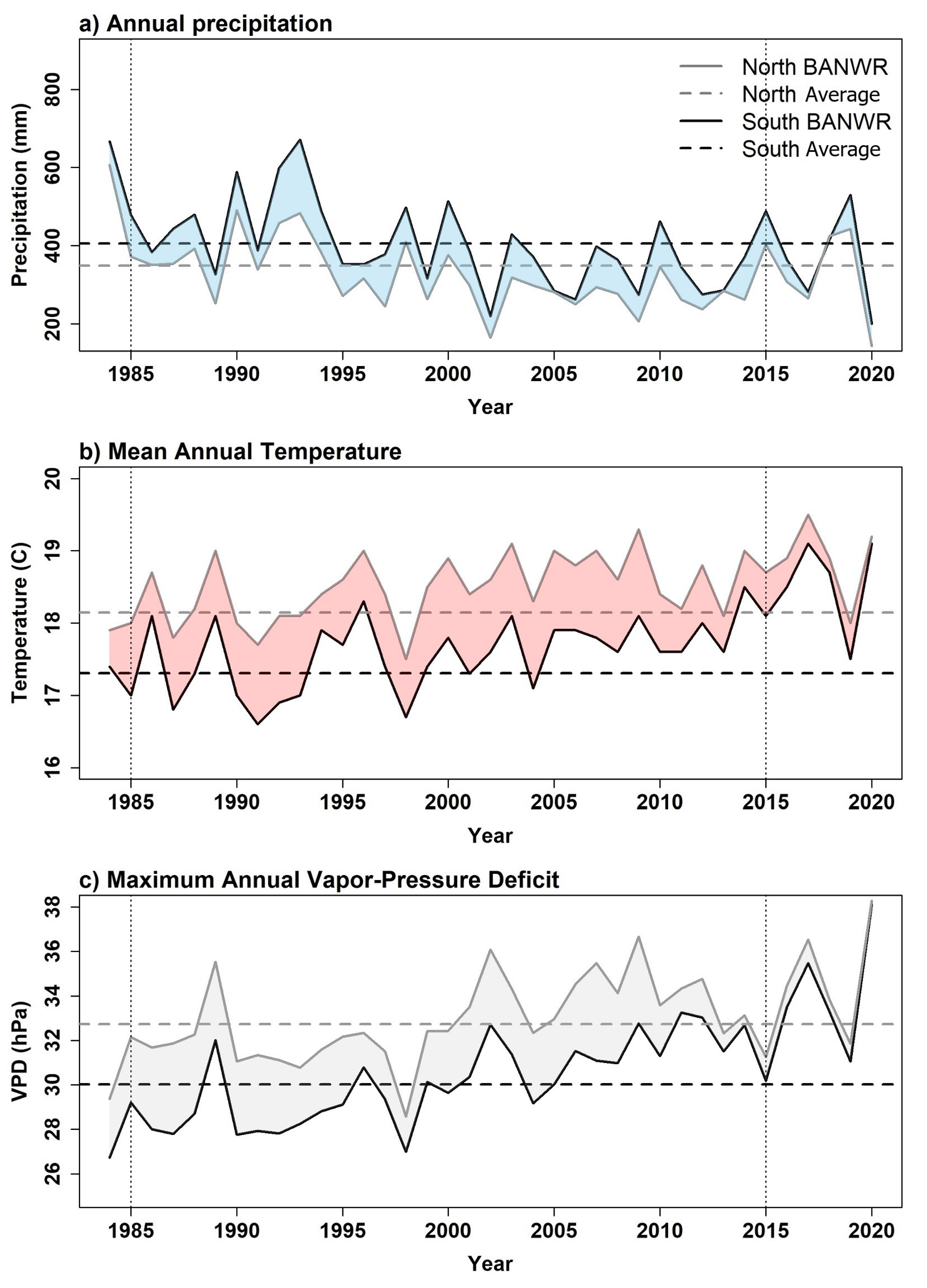
We characterized fine-fuel changes from 2015 to 2020 across the refuge and related these changes to previous wildfire and prescribed burns following the analysis steps outlined in Appendix A (Figure A1). We extracted records of fire locations, areal extent, estimated perimeter, type (i.e., wildfire or prescribed fire), cause, dates, and total area burned from the U.S. Fish and Wildlife Service’s Fire Management Information System (FMIS). We assessed pre- and post-fire treatment effects on the recovery timeframe of fine-fuels within perimeters of 12 fire incidents occurring between 2015 and 2020. To better understand the context of climate in relation to fuel trends over the study period, we obtained annual precipitation, mean annual temperature, and maximum annual vapor pressure deficit from the 4-km Parameter-elevation Regressions on Independent Slopes Model (PRISM) time series data [36,37]. Climate observations from the north and south ends of BANWR cover an increasing precipitation and decreasing temperature gradient from north to south. We compared these climatic trends against the annual trends in fine-fuels developed from remotely sensed imagery.
2.3. Remote Sensing Data
We used the Sentinel-2 mission products [32] obtained from either the European Space Agency’s Copernicus open access hub (https://scihub.copernicus.eu, accessed on 21 December 2020) or the USGS Earth Explorer (https://earthexplorer.usgs.gov, accessed on 21 December 2020) for development of imagery and data into serial models of fine-fuels. While the Sentinel-2 mission is currently composed of 2 satellite vehicles (A and B) with identically designed multi-spectral instruments, to maintain data continuity and consistent viewing geometry we used image data from only the Sentinel-2A sensor. Launched in 2015, the Sentinel-2A satellite remote sensing system and multi-spectral instrument is optimally configured for detecting plant productivity, with a total of 13 spectral bands, 6 of which are designed for capturing spectral response from vegetation [5,32]. Sentinel-2A is engineered for assessing vegetation attributes and change with two red-edge bands that record wavelengths in the transition zone between reflectance and absorption by chlorophyll [38]. Spectral channels and reflectance information provide a means to model fuels, assess fuel conditions over wide spatial extent with fine granular resolutions (10-m), and over long periods of time that are otherwise cost prohibitive using ground-based sampling [39].
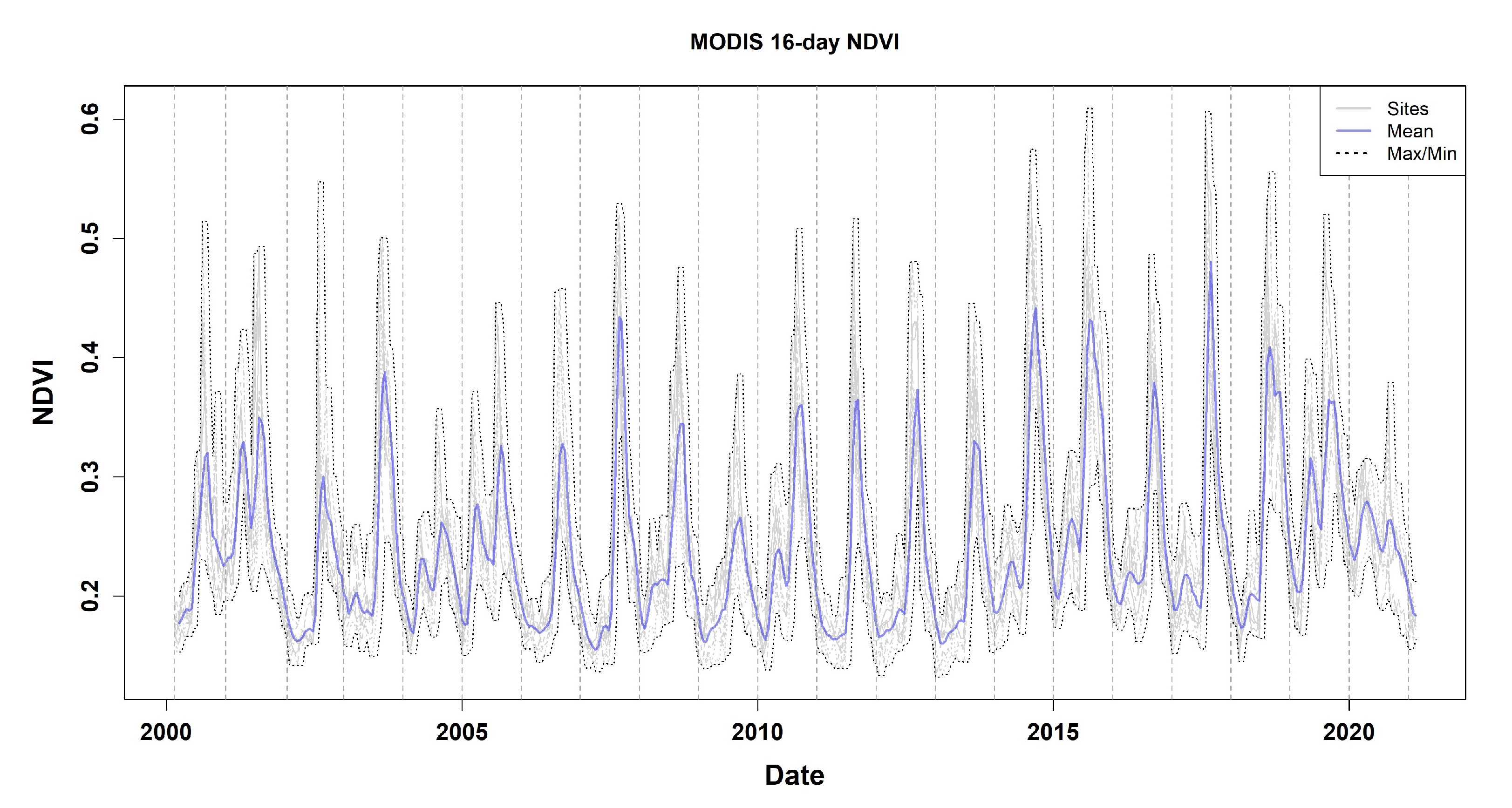
We acquired consistent seasonal image dates corresponding to peak greenness of vegetation (August) and autumn vegetation dormancy (November) periods from 2015 to 2020 with an ideal cloud cover threshold of less than 10%. We used 16-day averages of MODIS normalized difference vegetation index (NDVI) from 2000 to 2020 to determine the timing of peak vegetation greenness and vegetation dormancy of fine-fuels in our study area (Figure A2). While the lowest NDVI values were recorded during January (Figure A2), we opted to use autumn images to reduce likelihood of image contamination by clouds, snow, and natural decomposition of fine-fuels. Inclusion of images from both these time periods highlights the difference in spectral responses of intra-annual fine-fuel production. BANWR is geographically located along a seam between Sentinel-2A image footprints; two images were required for each time period for a total of 4 images per year, or 24 images over 6 years. We pre-processed level 1C products to level 2A using Sen2Cor software v. 2.8 to convert top-of-atmosphere reflectance values to surface reflectance [40]. We applied a cirrus correction, bidirectional reflectance distribution functions correction, and a terrain correction using the shuttle radar topography mission (SRTM) digital elevation model (DEM). Level 2A products were geometrically resampled (60 m and 20 m) to 10 m resolution across all the bands, then subset to bands of interest for further processing in ENVI Classic 5.5.3 (Exelis Visual Information Solutions, Boulder, CO, USA). Stacked images of overlapping scenes for each unique date were mosaicked and radiometrically normalized for consistency across time series to the 2015 baseline image. The intermediate step in radiometric normalization of multivariate alteration detection was performed with 3rd party plug-ins [41]. This step provided the desired image consistency and spectral band information for developing models of fine-fuels.
In all, 11 of the 13 total Sentinel-2A bands available for each image during the peak greenness of vegetation and vegetation dormancy periods were included in the analysis. Two image acquisition dates per year, with 11 bands for each date, provided a total of 22 spectral bands used as predictor variables, which were included in the training and predictive portions of the analysis, as described below. Spectral band 1 (443 nm) and band 10 (1380 nm) were only used during the atmospheric correction to reduce aerosol and cirrus effects. We used bands 2–9, 11, and 12 for our analysis as described and provided by the European Space Agency [32]: band 2 (blue: central wavelength = 490 nm, bandwidth = 65 nm), band 3 (green: central wavelength= 560 nm, width = 35 nm), band 4 (red: central wavelength = 665 nm, width = 30 nm), band 5 (vegetation red-edge 1: central wavelength = 705 nm, width = 15 nm), band 6 (vegetation red-edge 2: central wavelength = 740 nm, width = 15 nm), band 7 (vegetation red-edge 3: central wavelength = 783 nm, width = 20 nm), band 8 (near infrared 1: central wavelength = 842 nm, width = 115 nm), band 8a (near infrared 2: central wavelength = 865 nm, width = 20), band 9 (water vapor: central wavelength = 945 nm, width = 20 nm), band 11 (shortwave infrared 1: central wavelength = 1610 nm, width = 90), and band 12 (shortwave infrared 2: central wavelength = 2190 nm, width = 180 nm). We exclusively utilized spectral data in our analysis to simplify repeat processing and expand our ability to infer model results across space and time.
2.4. Modeling Fine-Fuels
To model fine-fuels, we used 2015 seasonal image dates together with cover and herbaceous biomass estimates from 20-m × 50-m field plots (n = 446) collected during the growing season in 2012 and 2015 [25,42]. In each plot, herbaceous vegetation cover was estimated using line-point intercept along six evenly spaced 20-m transects, with intercepts occurring at 0.5-m intervals. These cover measurements were related to clipped herbaceous biomass that fell within 0.5-m × 0.5-m quadrats spaced 5 m apart along the six 20-m transects at a subset of plots. These field-based estimates of biomass of fine-fuel (kg/ha) provided the dependent response variable for analysis. To align the models to the field-based data, we subset and processed the 2015 Sentinel-2A images to the study area extent and resampled images to spatially align image pixels. We then extracted average spectral values from field plot locations for use as model covariates treating individual bands as separate predictor variables. We randomly selected the field-based data, based on an 80/20 percent split, for model training and testing, respectively. We fed the combined spectral and vegetation information into program R statistical software v.3.6.3 [43] and the Classification and Regression Training (caret) package [44] to capitalize on machine learning methods. Recursive feature elimination was applied to reduce the set of potential predictor variables based on a 10-fold cross validation of lowest root mean square error (RMSE). Using the best predictor variables retained after recursive feature elimination, we developed spatial predictions of fine-fuel (kg/ha) with the random forest method in the caret package. We used the 20% reserved field-based (observed) testing data to fit a linear model against predictions for the training year (2015) and calculated the adjusted R-squared to examine model fit and accuracy. Subsequently, we predicted fine-fuel abundance and distribution for each year through 2020, based on the 2015 model, for the whole of BANWR.
2.5. Model Validation
To assess the accuracy and robustness of the fine-fuel models, we compared the first predicted year (2015) and the last predicted year (2020) of the fine-fuel models to temporally distinct field-based estimates of fine-fuels. For the first predicted year (2015), we used the 20% testing group data to compare field estimates of biomass with spatial predictions created by the random forest model with the caret package in program R. To assess the robustness of the predictability of fine-fuels derived from Sentinel-2A imagery and modeling over multiple years, we validated model results a second time with field-based measurements collected at the end of the growing season in November 2020, our final year of predictions of fine-fuels. To validate the last predicted year (2020), we stratified the study area for sampling using our 2019 Sentinel-2A estimates of fine-fuel abundance into low, medium, and high categories along with high to low topographic position index derived from SRTM DEM [45]. We visited and geolocated (Trimble R6 RTK-GPS rover and base station) two 80-m × 80-m field sites within each of the three fine-fuel strata for a total of 6 field sites. We visually estimated percent canopy cover of herbaceous vegetation at five or six 2-m × 2-m plots at each site (n = 35) based on 0.5-m × 0.5-m quadrats (n = 140) nested within plots. We then used these 2-m × 2-m plot estimates of field-based fine-fuel to validate the 2020 predicted fine-fuel models derived from the 2020 Sentinel-2A imagery using linear regression.
2.6. Fine-Fuel Changes
The 2015 to 2020 annual estimates of fine-fuel, developed with 2015 Sentinel-2A spectral characteristics and matching 2015 fine-fuels plots, were used to examine the effects of wildfire and prescribed fire on fuel loads. To assess recovery of fine-fuels, we compared fine-fuel from our Sentinel-2A derived model for pre- and post-fire years within burned area polygons obtained from FMIS. Within each wildfire and prescribed fire perimeter occurring between 2015 and 2020 (n = 12), we calculated the mean, minimum, maximum, range, sum, and standard deviation of fine-fuel (kg/ha) for each pre- and post-fire year. We then calculated the duration of time that elapsed until estimates of predicted biomass of fine-fuel post fire met and or exceeded pre-fire estimates. These descriptive metrics of burned area polygons were compared to fine-fuel metrics taken from unburned control areas that were within a 1-km buffer area of the fire perimeter, offering evidence of fire effects in a case-control design. We used a 1-km buffer to constrain our comparison to areas that were close to the fire and representative of similar vegetation types that existed within the burned area prior to the fire. Likewise, we constrained our analysis to only those portions of the larger fires shown in Figure 1 that intersected BANWR. We calculated change in estimated fine-fuels for annual time steps since year of fire and tested for cumulative differences in changes of fine-fuels between burned and unburned control areas with a 1-tailed t-test.
3. Results
Since 1985, prescribed fires accounted for 65% of fire events recorded at BANWR in the FMIS database (n = 133, average size = 646 ha) and wildfires (n = 71, mean size = 319 ha) accounted for the remaining 35%. Since 2015, 8 of the 12 fires recorded in the FMIS database were wildfires and 4 were prescribed fires (Table A1). Of the eight wildfires, half were ignited by natural and half by anthropogenic sources. Three of the four prescribed fires were conducted in March and one was implemented in June. One of the eight wildfires occurred in May, one in June, two in July, three in August, and one in December (Table A1). Our 2015 to 2020 study occurred during a period of fluctuating annual precipitation with record low annual precipitation in 2020 (Figure 2a), high mean annual temperature (Figure 2b), and high maximum annual vapor pressure deficit (Figure 2c) in both the southern and northern part of the refuge, relative to the 1985 to 2014 historical record. Notably, in 2019, the study area experienced above average precipitation and cool temperatures that promoted low-fire behavior. Two wildfires were reported in 2019, both of which represented the smaller acreages burned during the study timeframe. Conversely, in 2020, the study area experienced record-setting low summer monsoon precipitation, above average temperatures, and high vapor-pressure deficit (Figure 2).
Results from training of the 2015 fine-fuel model indicated an optimal RMSE of 500 kg/ha and an adjusted-R = 0.41 for the final random forest model based on internal cross validation. The top five variables included in the 2015 training model included: band 11 (shortwave infrared) during vegetation dormancy, and band 5 (red-edge), band 4 (red), band 8 (near infrared), and band 6 (red-edge) during peak greenness of vegetation, as shown in Table 1. Variable importance values indicated the percent increase in RMSE with predictors iterated in and out of the model. Of the 20 spectral variables included in the model, 12 of 20 were from the time period of peak greenness of vegetation while the other 8 were from vegetation dormancy. Total variable importance from spectral bands measured during peak greenness of vegetation accounted for 0.68 of overall importance, while spectral responses measured during vegetation dormancy accounted for 0.32. Subsequent spatial predictions for fine-fuel models from 2016 to 2015 were based on these variables.
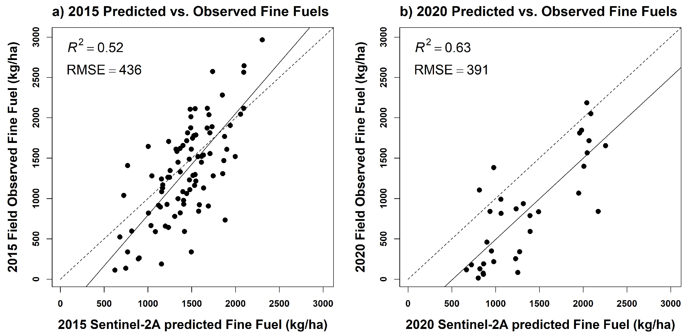
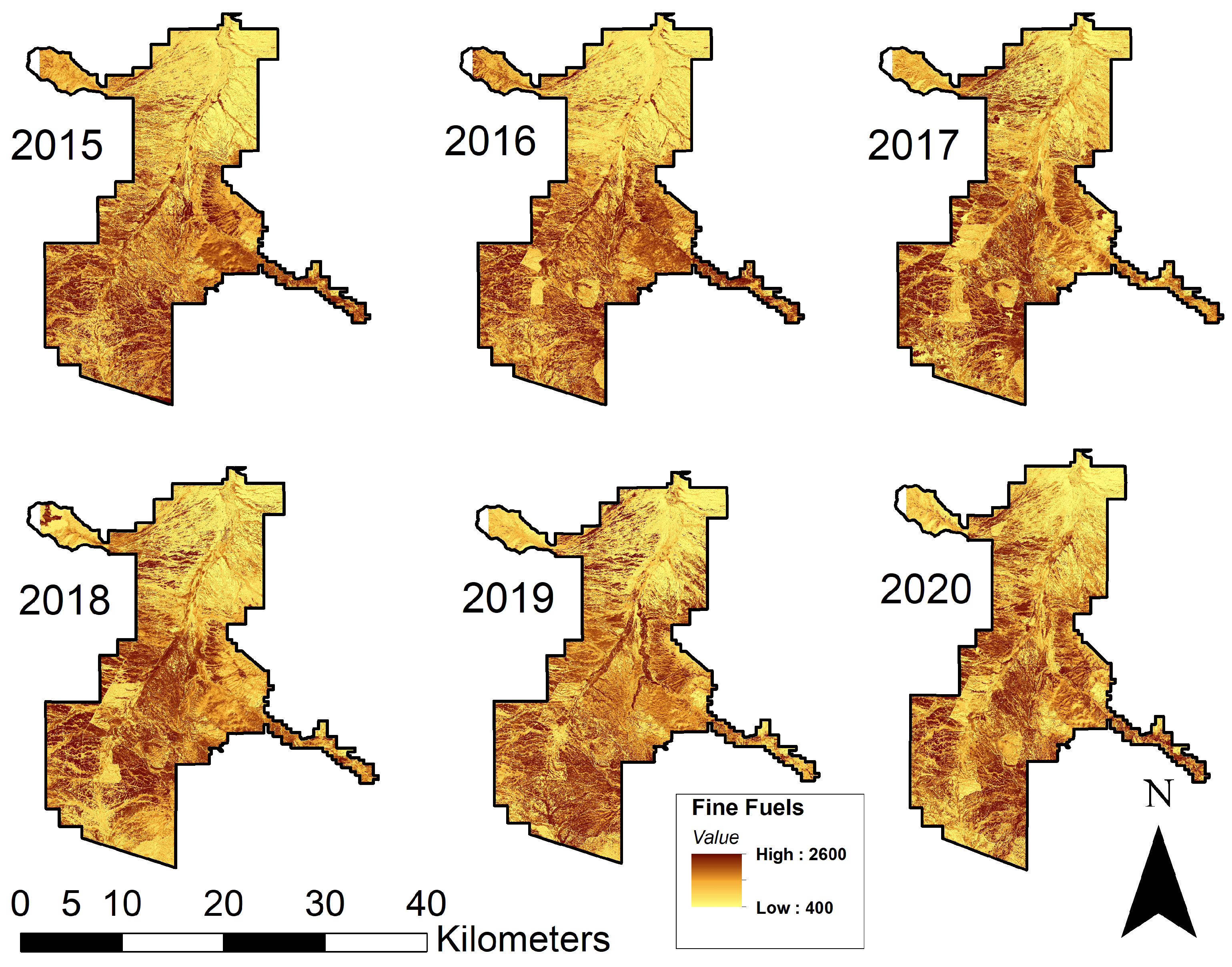
When compared with the 20% reserved testing data that we withheld to validate and assess model accuracy (separate from internal model training cross validation), the 2015 fine-fuel model (Figure 3a) had an adjusted-R of 0.52 (F = 93.62, p < 0.0001). The accuracy of the 2020 fine-fuel model based on its relation to the 2020 field-based measurements (R = 0.63, Figure 3b) was similar to that of 2015 and demonstrated the robustness of the model over time. The fine-fuel models provided continuous estimates of fine-fuels from lows of 200–400 kg/ha to highs of 2600–2800 kg/ha throughout BANWR (Figure 4). The annual series of Sentinel-2A derived models was used to map the yearly abundance and distribution of fine-fuels (kg/ha) at a 10-m resolution for BANWR (Figure 4 and Figure 5). For all years, fine-fuel data layers generally showed increasing values in a north to south direction, which was associated with increased elevation, increased precipitation, and cooler temperatures in the southern portion of the study refuge (Figure 2). The minimum and maximum amount of fine-fuel per year were generally within ±200 kg/ha of each other. Across the study area, fine-fuel was visibly reduced within fire perimeters following a fire event or treatment.
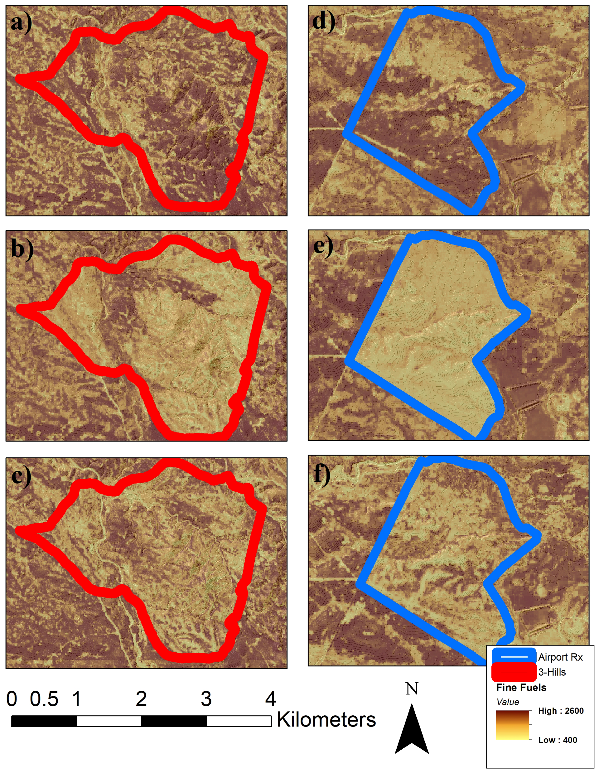
Close examination of two fire events, the 3-Hills wildfire (Figure 5a–c) and 2016 Airport prescribed fire (Figure 5d–f), showed high fine-fuel loads prior to ignition (Figure 5a,d), with visible reductions in the first-year post fire (Figure 5b,e). The 2016 Airport prescribed fire resulted in an average reduction of −660 kg/ha the first-year post fire, while the 3-Hills wildfire produced an average reduction of −480 kg/ha. The prescribed fire showed a homogeneous burn pattern and nearly complete overall reduction in fuels. Careful examination also revealed intentional and strategic prescribed burn patterning with greater reduction of fuels along ridge tops and benches, whilst lower reductions were achieved in areas of lower topography. The third-year post fire clearly showed a recovery of fuels, although not to the extent of pre-fire conditions (Figure 5c,f).
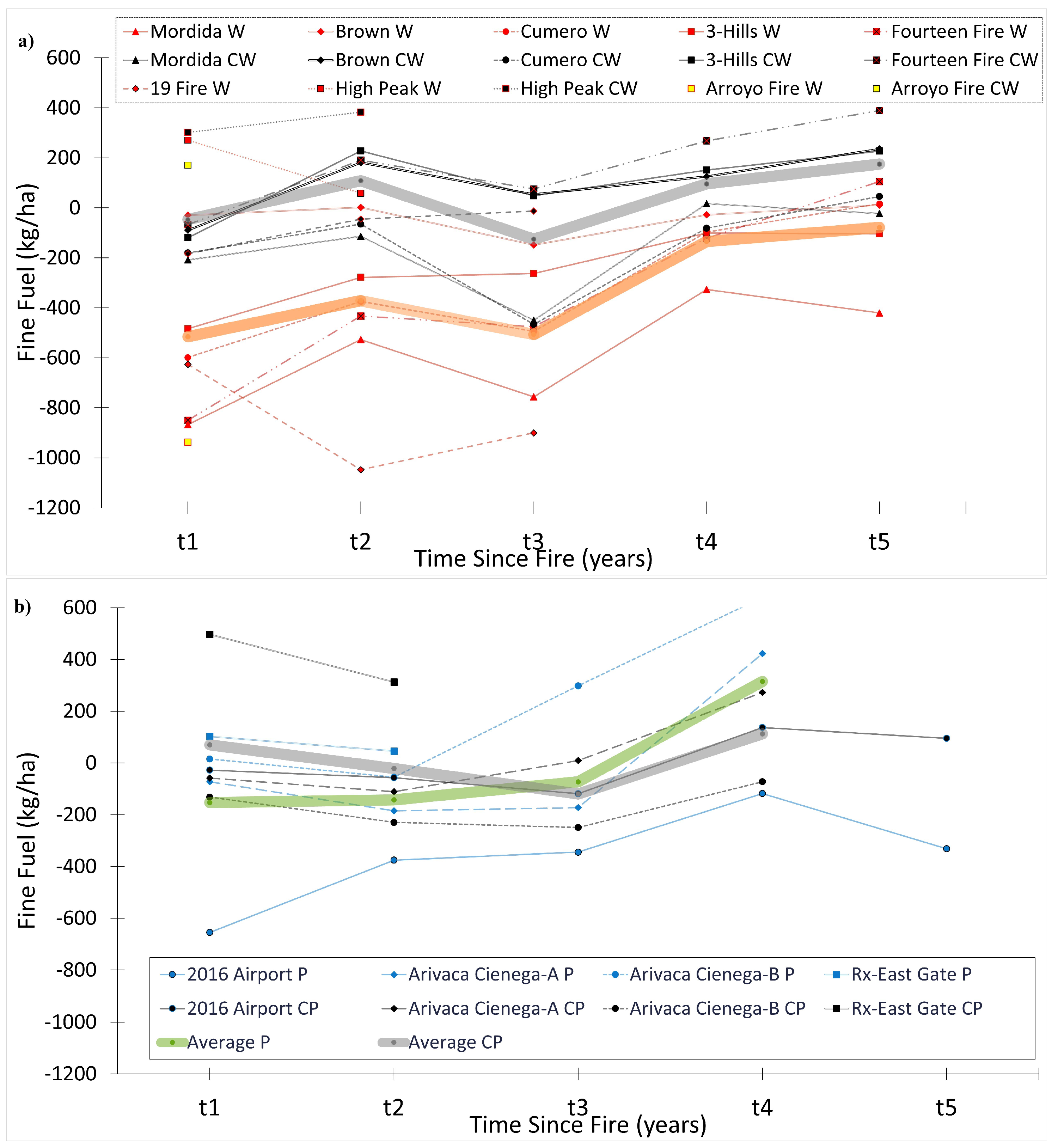
When 2015 to 2020 fires were compared to controls by year, wildfires tended to show greater impacts to fine-fuels than prescribed fires with greater difference between averages (Table A1) and greater differences between standard deviations (Table A2) in estimates of fine-fuel. Annualized since time of fire, there were greater average reductions due to wildfire (−516 kg/ha) compared to prescribed fire (−152 kg/ha) in the first-year post fire (Figure 6, Table A3 and Table A4). In contrast, unburned control plots in the first-year post fire showed virtually no change in fine-fuel estimates (−8 kg/ha). From 2015 to 2020, average values of fine-fuels estimated within burned areas tended to be lower (Table A1), and with lower variation (Table A2), than unburned reference plots. Notable exceptions to the expected reductions of fine-fuel included both the 2019 High Peak wildfire and the 2019 East Gate Border Patrol prescribed fire in which both had increases in estimates of fine-fuels the first-year post fire (Table A4 and Figure 6). Higher than expected fuel in 2019 was likely due to above average annual precipitation (Figure 2), as even the unburned control plots increased by 220 kg/ha in 2019.
When grouped by years, the combined metrics of fuel reduction for prescribed fire and wildfire showed a significant difference in post-fire fuel loads for up to 5 years post fire based on a one-tailed t-test with unequal variances (t = 1.67, p < 0.00001). Following the immediate reduction in fine-fuels one-year post fire (n = 12, µ = −394 kg/ha), there was a gradual increase in fine-fuels with return to pre-fire levels between 3 and 5 years (Table A4). Second-year post-fire average reductions (n = 11, µ = −288 kg/ha) in estimates of fine-fuels were about 3/4 of first-year reductions. Average reductions of fine-fuels (n = 9, µ = −294 kg/ha) in the third year were similar to second-year reductions and 3/4 of first-year reductions, on average. Fourth-year estimates of average yearly changes in fine-fuel surpassed initial pre-fire conditions (n = 8, µ = 54 kg/ha) with fifth-year estimates slightly below. Individually, some fire treatment areas showed recovery of estimated fine-fuels to pre-treatment levels within 1–2 years and upwards of 5 years.
The individual effect of fires on burned area polygons varied due to treatment type, a reflection of seasonality, timing, and burning objectives. Average reductions in fine-fuels by wildfire events tended to be much greater on average than those of prescribed fires (Table A4). Although, with a Bonferroni adjustment that shifted significant p-values from 0.05 to 0.0125 for multiple tests (4 years), there were no statistically significant differences for prescribed fire and wildfire in post-fire years and the comparisons were hampered by low and diminishing sample size over time. When fire types (prescribed fire and wildfire) were grouped and burned areas were compared to unburned control plots, yearly differences were significant. One-tailed t-tailed tests with Bonferroni adjustments revealed significant differences in the first (t = −2.80, p = 0.006) and second year (t = −3.03, p < 0.0001) post fire. Third (t = −1.73, p = 0.054), fourth (t = −0.55, p = 0.30), and fifth (t = −2.67, p = 0.01) post-fire years were not significantly different with Bonferroni adjustments in average fuel reductions due to fire; however, sample size was halved by year 5 and a greater proportion of year 3–5 post-fire samples included 2019, a year of enhanced productivity.
4. Discussion
With increases in wildfire activity in recent decades [1,2], there is a growing need for an accurate, updateable, and expandable model of fine-fuels. Our annual estimates of fine-fuel across a wildlife refuge in southern Arizona provide spatially explicit information for fire-risk mitigation strategies, wildlife management, and to further our understanding of the ecological outcomes of wildfire and prescribed fire in non-forested ecosystems. Determining the contemporary trends of fine-fuels and their response to fire on the refuge can help inform fuel treatments in similar systems that have undergone invasion by non-native grasses and experienced a legacy of different land uses. As expected, areas within the refuge that experienced both prescribed fire and wildfire showed substantial reduction in estimates of fine-fuels the first year following fire and recovered to pre-fire levels within 3–5 years. Our comparison with unburned control areas suggests that fuel conditions may fluctuate less widely between years than previously expected, with wildfire having a greater impact on fuel reductions (−520 kg/ha) than prescribed fire (−160 kg/ha).
Our study demonstrates that Sentinel-2A imagery can produce spatially explicit fine-fuel estimates at relatively high spectral (13 bands) and spatial resolution (10 m) over a broad spatial extent (40 km × 30 km). These improvements are necessary to assess pre- and post-fire conditions and evaluate fuel treatment efficacy and longevity. Previous efforts to map fuels in arid and semi-arid regions have typically relied on coarse to moderate resolution imagery [42,46,47] or focused on generating high-resolution predictions within a narrow study region of interest [48,49]. The increased resolution and spatial extent of fuel estimates in our study are more suitable for fuel management planning and decision making. The relatively high resolution of our fuel estimates is particularly important for the patchy and heterogenous fine-fuel in semi-arid grasslands, which is in contrast to the more traditionally studied continuous and homogenous fine-fuels of more mesic systems [50]. Due to the ongoing, publicly available data collection by the Sentinel-2 mission, the methodology we implemented is updateable and applicable to other ecosystems where improvements to fine-fuel monitoring is needed.
Our model estimates of fine-fuels showed positive linear agreement with validation data in both 2015 (adjusted-R = 0.52) and 2020 (adjusted-R = 0.63) with some sources of unexplained variation (Figure 3). The 2020 model showed slight bias towards over predicting fine-fuel, which may be due to the acquisition of 2020 images 2 weeks later in the growing season compared to the 2015 training year. Additional unexplained variation may be attributable to a resolution mismatch between the image predicted (10 m) and field observed (2 m) estimates of fine-fuel. Nonetheless, the number of variables we included in model parameterization was far less than previous efforts [42], which reduces overfitting of models, a potential drawback of machine learning methods that results in the inability to predict future observations reliably. Although additional variables such as vegetation and soil indices may increase model accuracy, our multi-year validation allowed for the reliable development of a time series of fine-fuel estimates. Key elements of our analysis that allowed for this time series included rigorous image corrections and radiometric normalizations to match spectral data across scenes and years. Our model results expand on other remote sensing studies that show the importance of shortwave and near-infrared bands for characterizing vegetation dynamics in grasslands and other drylands, especially where biomass is largely composed of non-photosynthetic vegetation [51,52]. Our models also show that considering spectral information during both peak vegetation greenness and vegetation dormancy can improve estimates of fine-fuels in grasslands and other drylands. Assessment of grassland fuels is particularly important in the context of invasive annual and perennial grasses that may show high interannual variation in fuel hazard [53,54]. We found that the spectral range and frequent return interval of the Sentinel-2A vehicle (10-day return interval) was compatible with yearly fine-fuel monitoring objectives and expect the Sentinel-2B vehicle to achieve similar results, offering a combined 5-day return interval of the Sentinel-2 mission.
Our fuel models can be readily employed to monitor fine-fuel changes over multiple years, which is an improvement from a previous one-year assessment [42]. This progress is necessary to detect fine-fuel changes attributable to climate, land-use, and fire conditions. For example, our time series accommodated the large interannual climate variability of the 2015–2020 study period, which included wetter (2019) and much drier (2020) than average conditions in consecutive years. This detection of year-to-year variation can largely be attributable to conducting field validations in both wet (2015) and very dry (2020) years. Our models will be useful moving forward as 2021 is one of the wettest summers on record and will likely create high fine-fuel loads and additional wildfire risk, especially if a subsequent dry year elevates flammability. Indeed, drier conditions interspersed with periods of more intense rainfall is the forecasted trend for the southwestern U.S. [55,56] and is likely to create additional fire risk that our models can help inform.
Our study area is widely representative of increasingly fire prone drylands throughout the western U.S. and world [10,57] due to invasion by non-native grasses [7,17]. While we did not specifically account for the differences in non-native and native grass contributions to fine-fuels, our estimates of fuel load within 2015–2020 burn perimeters (1400–1800 kg/ha) are twice the previous estimates of Lehman lovegrass invaded semi-arid grasslands in southeastern Arizona in dry summers (900 kg/ha) and considerably higher than the fine-fuel in native semi-arid grasslands in the region (300–700 kg/ha) (Cox et al. 1990). Non-native lovegrasses, introduced to provide erosion control and forage, have proliferated over vast parts of the refuge and semi-arid grasslands in the region over the last several decades and have enhanced fire continuity and spread [58]. Their general high tolerance to drought and livestock grazing [59], which is widespread in areas adjacent to the refuge, indicate that they will continue to present wildfire risk in the future. Although the refuge has not experienced livestock grazing since 1985, future studies can compare how fuel load from native and non-native invasive grasses changes with grazing and other land-uses.
While our results indicate reductions in fine-fuel for up to three years due to prescribed burning, previous studies have suggested that invasive lovegrasses may increase or show no change, in relation to decreased abundance of native grasses, even when fire return intervals are frequent [52,60,61]. Beginning one-year post fire, our analysis showed a regeneration of fine-fuels after prescribed fire surpassing pre-fire fine-fuel estimates in the third to fourth year post fire (Figure 6b). Future prescribed fires can balance the need for a longer recovery time of native grasses, and the habitat requirements of masked bobwhite quail, with the need to manage fire risk. Our results generally indicate areas of patchy high fine-fuel abundance, which is consistent with the preference of Lehmann lovegrass occurring on soils of high sand and low clay content [62] and the biophysical relationships of fire distribution of grasslands in the southwestern U.S. [63]. These and other environmental conditions that increase the abundance of Lehmann lovegrass and associated fine-fuels can be incorporated into future burn plans [64]. Further analysis of Sentinel-2A imagery in the manner described herein may eventually allow for biophysical-spectral mapping of Lehmann lovegrass dominated sites, allowing for greater quantification and characterization of the threat of invasive grasses.
Our study demonstrated that wildfire decreased fuel by three times the amount of prescribed fire and increased the length of time until fine-fuels approach pre-fire estimates (Figure 6). This difference is largely because prescribed burning typically happens under the cooler and relatively wetter conditions in the spring, which reduces the risk of unwanted spread but leads to less fuel consumed than the hotter and drier conditions of summer wildfires [65]. An exception was the 2016 Airport prescribed fire that consumed an amount of fine-fuel comparable to most wildfires on the refuge due to its ignition in June. While recent calls for more prescribed fire [21] may be necessary in many over-crowded forests and grasslands encroached on by woody species, burn plans in drylands invaded by non-native flammable species should carefully weigh the cost of increasing fire return interval and continued spread of the non-native species. These invasions may result in unfavorable wildlife habitat and lead to land degradation.
The range of 3 to 5 years needed for recovery of fine-fuels that we found in our study is likely influenced by the seasonality and size of the burn and annual climate. For example, the slight increase in fine-fuels the year following fire in 2019 was likely due to above average precipitation, the late-winter timing of the prescribed East Gate fire, and the limited areal extent of the High Peak (3.4 ha) fire. Winter burning combined with favorable spring growing conditions promotes plant recruitment and growth, thereby enhancing fine-fuels, especially with the presence of invasive grasses. The relatively short recovery period of fine-fuels found in our study supports previous findings of semi-arid grassland fires [16,66,67]. Although we expected higher interannual variability of fine-fuels associated with climatic fluctuations, the variability was relatively low and might be explained by the high resilience of grasses to fire, the dominance of perennial grasses in our study area that have lower interannual changes than annual grasses, and the maintenance of fuel through time by the highly productive invasive Lehmann lovegrass.
Our results provide a means for fire managers to prioritize strategic actions where critical natural resource values, infrastructure, and human health are at stake. Updateable, high-resolution fine-fuel maps allow for managers to move from a reactive approach to a proactive data-driven approach that can be used in an adaptive framework [68] to better understand and manage potentially hazardous fuels through time. Additionally, these annual fuel layers can be overlaid with other data relevant to assessment of values at risk, such as critical habitat for endangered species (e.g., masked bobwhite quail at BANWR) or areas of high erosion potential, to help coordinate prescribed burning and other treatments. Our fuel models represent an important testing and calibrating opportunity for verification of simulations of fire behavior outputs [69] that have historically not performed well under conditions of patchy and heterogenous fuels in drylands [50].
In particular, our fine-fuel model is geared toward use in next-generation fire simulation programs such as the QUIC-Fire (Linn et al., 2020) tool for prescribed fire planning that allows for inclusion of a continuous fine-scale model of surface fuels. Our fuel models of BANWR represent an important testing and calibrating opportunity for wildfire simulations and an opportunity to implement an adaptive management approach to refuge operations, including on-going efforts to improve the population viability of the masked bobwhite quail. Past prescribed fires that have known ignition and spread patterns can be analyzed to help calibrate forecasting tools to better inform future burning outcomes based on fire weather and fine-fuel estimates. When observed versus modeled fuel and fire simulations are iteratively tested, they can be used to plan future treatment scenarios with otherwise unknowable outcomes. Our study provides an avenue for potential integration of updateable fine-fuels across dryland ecosystems more broadly, to formulate a better understanding of fire risk and fuel treatment outcomes in the western U.S. and throughout the world.
5. Conclusions
We demonstrated the development of high-resolution estimates of fine-fuel across a semi-arid grassland to assess the effects of prescribed fire and wildfire through time. We employed Sentinel-2A imagery in the vegetation growing and dormant seasons, and machine learning analyses, to predict annual increments of fine-fuels from 2015 to 2020. Using field-collected biomass data in 2015 and 2020, we validated our predictions and found reasonable agreement between predicted and observed estimates of fine-fuels (R = 0.52–0.63). When our fine-fuel time series was overlaid with historical burns, we found one-year post-fire reductions of −160 kg/ha and −560 kg/ha of prescribed fire and wildfire, respectively, with subsequent recovery of fuel loads within 3–5 years. Our remote sensing-based method can save on time and resources required to monitor fuel loads in the field and is readily updateable to assess rapid changes in fuel conditions to support fire and natural resource management at scales of 10s to 1000s of hectares on an annual basis. Further research can expand the development of high-resolution models of fine-fuels across dryland landscapes to support national and continental level mapping efforts.
Author Contributions
Conceptualization, S.M.M., S.E.S., and M.L.V.; methodology, S.E.S.; software, S.E.S., and A.G.W.; validation, A.G.W., S.E.S., and S.M.M.; formal analysis, A.G.W.; investigation, A.G.W., S.E.S., S.M.M., and M.L.V.; resources, S.M.M., and S.E.S. data curation, A.G.W.; writing—original draft preparation, A.G.W.; writing—review and editing, S.M.M., S.E.S., and M.L.V.; visualization, A.G.W., and S.E.S. supervision, S.M.M., S.E.S., and M.L.V.; project administration, S.M.M., and S.E.S.; funding acquisition, S.M.M., M.L.V., and S.E.S. All authors have read and agreed to the published version of the manuscript.
Funding
This work was supported by the U.S. Geological Survey Wildland Fire Science Program within the Ecosystems Mission Area, the U.S. Fish and Wildlife Service, the Department of the Interior Office of Wildland Fire, and the Department of Homeland Security U.S. Customs and Border Patrol. The Joint Fire Science Program funded previous fine-fuels data collection through grant number 13-1-06-16.
Institutional Review Board Statement
Not applicable.
Informed Consent Statement
Not applicable.
Data Availability Statement
The data that support the findings of this study are publicly available at the USGS ScienceBase-Catalog https://0-doi-org.brum.beds.ac.uk/10.5066/P91U530P [70].
Acknowledgments
We thank Paul Steblein, Brent Range, Jeff Rupert, Craig Leff, Joel Sankey, Josh Caster, Kevin Hiers, and the staff at Buenos Aires National Wildlife Refuge for providing useful advice and assistance on this study. The findings and conclusions in this manuscript are those of the authors and do not necessarily represent views of the U.S. Fish and Wildlife Service. Any use of trade, product, or firm names in this article is for descriptive purposes only and does not imply endorsement by the U.S. government.
Conflicts of Interest
The authors declare no conflict of interest. The funders had no role in the design of the study; in the collection, analyses, or interpretation of data; in the writing of the manuscript; or in the decision to publish the results.
Abbreviations
The following abbreviations are used in this manuscript:
| BANWR | Buenos Aires National Wildlife Refuge |
| caret | Classification and Regression Training |
| DEM | Digital Elevation Model |
| FMIS | Fire Management Information System |
| MODIS | Moderate Resolution Imaging Spectroradiometer |
| NDVI | Normalized Difference Vegetation Index |
| PRISM | Parameter-elevation Regressions on Independent Slopes Model |
| RMSE | Root Mean Square Error |
| SPOT | Satellite Pour l’Observation de la Terre |
| SRTM | Shuttle Radar Topography Mission |
Appendix A
Figure A1.
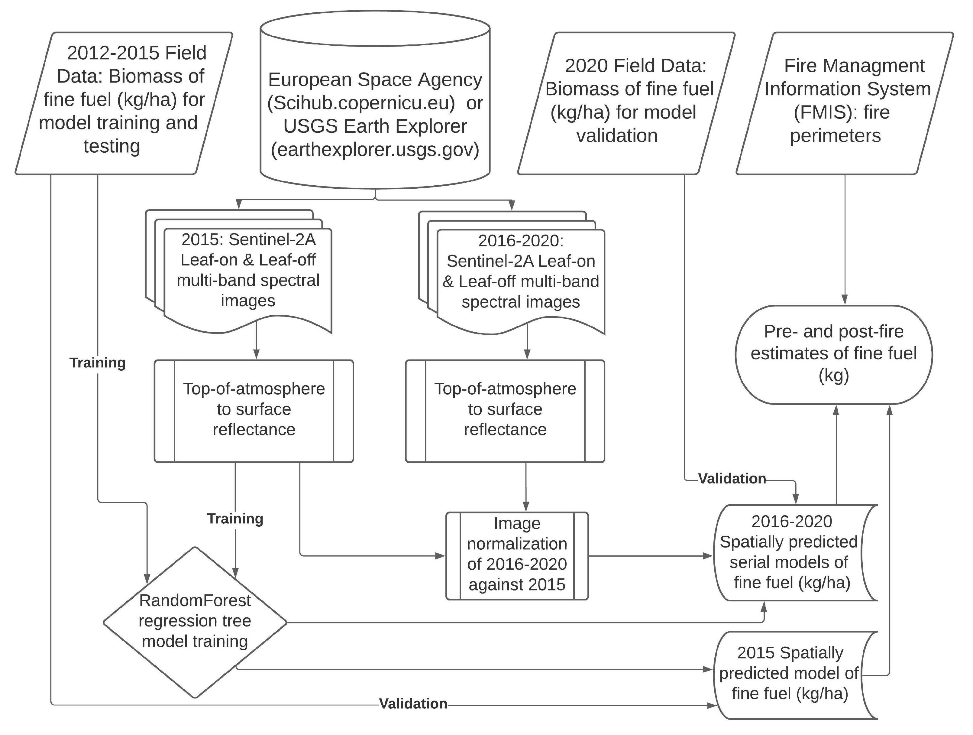
Analysis flowchart showing input data and processing steps for estimating changes of fine-fuels (kg/ha) over time in relation to prescribed fire and wildfire.
Figure A1.
Analysis flowchart showing input data and processing steps for estimating changes of fine-fuels (kg/ha) over time in relation to prescribed fire and wildfire.

Figure A2.
Seasonal and annual normalized difference vegetation index (NDVI) patterns from the Moderate Resolution Imaging Spectroradiometer (MODIS) satellite sensor, showing the timing of peak vegetation greenness typically occurring in August (Julian date = 220) and post growing season dormant period beginning in November at BANWR.


Table A1.
The yearly estimated mean () of fine-fuels (kg/ha) within burn perimeters for wildfire (W) and prescribed (P) fires at BANWR, with parenthesized boldface values indicating pre-burn estimates prior to ignition (some ignition dates do not align with calendar date but rather to pre- or post-imagery dates) against 1-km buffered control (C) areas around fire perimeters (parenthesized italicized values reference ignition time period for unburned control samples).
| CASE: Fire Name | Type | Year | Date | 2015 | 2016 | 2017 | 2018 | 2019 | 2020 |
|---|---|---|---|---|---|---|---|---|---|
| 2016 Airport | P | 2016 | 06.07 | (1608) | 952 | 1232 | 1264 | 1490 | 1276 |
| Arivaca Cienega A | P | 2017 | 03.08 | 1662 | (1520) | 1448 | 1336 | 1348 | 1944 |
| Arivaca Cienega B | P | 2017 | 03.08 | 1554 | (1218) | 1232 | 1162 | 1516 | 1858 |
| RX-East Gate BP | P | 2019 | 03.05 | 1404 | 1312 | 1412 | (1248) | 1350 | 1294 |
| Fourteen Fire | W | 2015 | 08.22 | (1790) | 940 | 1356 | 1314 | 1668 | 1894 |
| Mordida | W | 2015 | 12.18 | (1758) | 892 | 1232 | 1002 | 1432 | 1338 |
| Brown | W | 2016 | 06.17 | (1284) | 1254 | 1286 | 1136 | 1256 | 1296 |
| Cumero | W | 2016 | 05.06 | (1672) | 1072 | 1296 | 1176 | 1574 | 1688 |
| Three Hills | W | 2016 | 07.21 | (1654) | 1172 | 1376 | 1392 | 1554 | 1550 |
| 19 Fire | W | 2018 | 08.07 | 1492 | 1338 | (1966) | 1338 | 918 | 1064 |
| High Peak | W | 2019 | 07.17 | 1458 | 1406 | 1182 | (1232) | 1504 | 1292 |
| Arroyo Fire | W | 2019 | 08.31 | 1642 | 1466 | 2104 | 1770 | (1914) | 978 |
| Average () | P | - | - | 1556 | 1250 | 1332 | 1252 | 1426 | 1592 |
| Average () | W | - | - | 1594 | 1192 | 1474 | 1296 | 1478 | 1388 |
| CONTROL | Type | Year | Date | 2015 | 2016 | 2017 | 2018 | 2019 | 2020 |
| 2016 Airport | CP | 2016 | NA | (1464) | 1436 | 1406 | 1346 | 1602 | 1560 |
| Arivaca Cienega A | CP | 2017 | NA | 1496 | (1464) | 1406 | 1354 | 1474 | 1738 |
| Arivaca Cienega B | CP | 2017 | NA | 1154 | (1262) | 1130 | 1032 | 1012 | 1190 |
| RX-East Gate BP | CP | 2019 | NA | 1376 | 1290 | 1426 | (1186) | 1682 | 1498 |
| Fourteen Fire | CW | 2015 | NA | (1398) | 1332 | 1590 | 1474 | 1666 | 1788 |
| Mordida | CW | 2015 | NA | (1578) | 1370 | 1462 | 1128 | 1596 | 1556 |
| Brown | CW | 2016 | NA | (1304) | 1214 | 1484 | 1356 | 1428 | 1538 |
| Cumero | CW | 2016 | NA | (1644) | 1462 | 1578 | 1176 | 1562 | 1688 |
| Three Hills | CW | 2016 | NA | (1544) | 1424 | 1772 | 1592 | 1694 | 1770 |
| 19 Fire | CW | 2018 | NA | 1226 | 1044 | (1510) | 1326 | 1464 | 1496 |
| High Peak | CW | 2019 | NA | 1580 | 1440 | 1388 | (1338) | 1640 | 1722 |
| Arroyo Fire | CW | 2019 | NA | 1378 | 1360 | 1682 | 1562 | (1636) | 1806 |
| Average () | CP | - | - | 1372 | 1364 | 1342 | 1230 | 1442 | 1496 |
| Average () | CW | - | - | 1456 | 1330 | 1558 | 1370 | 1586 | 1670 |
Table A2.
The yearly estimated standard deviation () of fine-fuels (kg/ha) within burn perimeters for wildfire (W) and prescribed (P) fires at BANWR, with parenthesized boldface values indicating pre-burn estimates prior to ignition (some ignition dates do not align with calendar date but rather to pre- or post-imagery dates) against 1-km buffered control (C) areas around fire perimeters (parenthesized italicized values reference ignition time period for unburned control samples).
| CASE: Fire Name | Type | Year | Date | 2015 | 2016 | 2017 | 2018 | 2019 | 2020 |
|---|---|---|---|---|---|---|---|---|---|
| 2016 Airport | P | 2016 | 06.07 | (344) | 148 | 212 | 276 | 314 | 118 |
| Arivaca Cienega A | P | 2017 | 03.08 | 218 | (220) | 176 | 196 | 256 | 362 |
| Arivaca Cienega B | P | 2017 | 03.08 | 308 | (202) | 264 | 212 | 330 | 282 |
| RX-East Gate BP | P | 2019 | 03.05 | 352 | 302 | 378 | (288) | 362 | 270 |
| Fourteen Fire | W | 2015 | 08.22 | (248) | 170 | 144 | 106 | 78 | 386 |
| Mordida | W | 2015 | 12.18 | (456) | 140 | 210 | 108 | 308 | 252 |
| Brown | W | 2016 | 06.17 | (180) | 232 | 172 | 326 | 232 | 296 |
| Cumero | W | 2016 | 05.06 | (320) | 174 | 160 | 156 | 352 | 254 |
| Three Hills | W | 2016 | 07.21 | (396) | 268 | 306 | 280 | 292 | 246 |
| 19 Fire | W | 2018 | 08.07 | 226 | 230 | (304) | 166 | 218 | 320 |
| High Peak | W | 2019 | 07.17 | 104 | 156 | 104 | (90) | 110 | 198 |
| Arroyo Fire | W | 2019 | 08.31 | 444 | 210 | 372 | 248 | (204) | 234 |
| St. Dev. () | P | - | - | 306 | 218 | 258 | 242 | 314 | 258 |
| St. Dev. () | W | - | - | 298 | 198 | 222 | 184 | 224 | 274 |
| CONTROL | Type | Year | Date | 2015 | 2016 | 2017 | 2018 | 2019 | 2020 |
| 2016 Airport | CP | 2016 | NA | (280) | 260 | 368 | 318 | 298 | 248 |
| Arivaca Cienega A | CP | 2017 | NA | 282 | (294) | 278 | 294 | 338 | 374 |
| Arivaca Cienega B | CP | 2017 | NA | 266 | (346) | 250 | 244 | 254 | 336 |
| RX-East Gate BP | CP | 2019 | NA | 338 | 280 | 340 | (156) | 322 | 342 |
| Fourteen Fire | CW | 2015 | NA | (330) | 210 | 360 | 196 | 170 | 354 |
| Mordida | CW | 2015 | NA | (392) | 292 | 304 | 218 | 306 | 288 |
| Brown | CW | 2016 | NA | (252) | 270 | 342 | 246 | 326 | 320 |
| Cumero | CW | 2016 | NA | (326) | 236 | 304 | 178 | 328 | 320 |
| Three Hills | CW | 2016 | NA | (372) | 284 | 414 | 302 | 294 | 358 |
| 19 Fire | CW | 2018 | NA | 336 | 296 | (450) | 316 | 416 | 328 |
| High Peak | CW | 2019 | NA | 144 | 132 | 190 | (148) | 140 | 238 |
| Arroyo Fire | CW | 2019 | NA | 358 | 226 | 394 | 318 | (230) | 280 |
| St. Dev. () | CP | - | - | 292 | 296 | 310 | 278 | 304 | 324 |
| St. Dev. () | CW | - | - | 314 | 244 | 346 | 240 | 276 | 310 |
Table A3.
The yearly estimated change () of fine-fuels (kg/ha) within burn perimeters after wildfire (W) and prescribed (P) fires at BANWR against 1-km buffered control (C) areas around fire perimeters (some ignition dates do not align with calendar date but rather to pre- or post-imagery dates).
Table A3.
The yearly estimated change () of fine-fuels (kg/ha) within burn perimeters after wildfire (W) and prescribed (P) fires at BANWR against 1-km buffered control (C) areas around fire perimeters (some ignition dates do not align with calendar date but rather to pre- or post-imagery dates).
| CASE: Fire Name | Type | Year | Date | 2015 | 2016 | 2017 | 2018 | 2019 | 2020 |
|---|---|---|---|---|---|---|---|---|---|
| 2016 Airport | P | 2016 | 06.07 | - | −654 | −376 | −344 | −118 | −332 |
| Arivaca Cienega A | P | 2017 | 03.08 | - | - | −72 | −184 | −172 | 422 |
| Arivaca Cienega B | P | 2017 | 03.08 | - | - | 16 | −56 | 298 | 640 |
| RX-East Gate BP | P | 2019 | 03.05 | - | - | - | - | 102 | 46 |
| Fourteen Fire | W | 2015 | 08.22 | - | −850 | −434 | −476 | −122 | 104 |
| Mordida | W | 2015 | 12.18 | - | −866 | −528 | −756 | −326 | −420 |
| Brown | W | 2016 | 06.17 | - | −30 | 2 | −148 | −28 | 12 |
| Cumero | W | 2016 | 05.06 | - | −598 | −374 | −494 | −96 | 16 |
| Three Hills | W | 2016 | 07.21 | - | −484 | −278 | −262 | −102 | −104 |
| 19 Fire | W | 2018 | 08.07 | - | - | - | −626 | −1048 | −900 |
| High Peak | W | 2019 | 07.17 | - | - | - | - | 270 | 58 |
| Arroyo Fire | W | 2019 | 08.31 | - | - | - | - | - | −938 |
| Average Change () | P | - | - | - | −654 | −144 | −194 | 28 | 194 |
| Average Change () | W | - | - | - | −566 | −322 | −460 | −208 | −272 |
| CONTROL | Type | Year | Date | 2015 | 2016 | 2017 | 2018 | 2019 | 2020 |
| 2016 Airport | CP | 2016 | NA | - | −28 | −58 | −118 | 138 | 96 |
| Arivaca Cienega A | CP | 2017 | NA | - | - | −58 | −110 | 10 | 272 |
| Arivaca Cienega B | CP | 2017 | NA | - | - | −132 | −230 | −250 | −72 |
| RX-East Gate BP | CP | 2019 | NA | - | - | - | - | 496 | 314 |
| Fourteen Fire | CW | 2015 | NA | - | −68 | 190 | 76 | 268 | 390 |
| Mordida | CW | 2015 | NA | - | −208 | −114 | −450 | 16 | −22 |
| Brown | CW | 2016 | NA | - | −90 | 182 | 54 | 124 | 236 |
| Cumero | CW | 2016 | NA | - | −180 | −66 | −466 | −82 | 46 |
| Three Hills | CW | 2016 | NA | - | −120 | 228 | 48 | 152 | 226 |
| 19 Fire | CW | 2018 | NA | - | - | - | −184 | −46 | −14 |
| High Peak | CW | 2019 | NA | - | - | - | - | 302 | 384 |
| Arroyo Fire | CW | 2019 | NA | - | - | - | - | - | 170 |
| Average Change () | CP | - | - | - | −28 | −82 | −152 | 98 | 152 |
| Average Change () | CW | - | - | - | −132 | 84 | −154 | 106 | 176 |
Table A4.
Annual changes in estimates of fine-fuels (kg/ha) since time (t) of ignition for prescribed fire (P) and wildfire (W) relative to control (C) areas from 2015 to 2020 at BANWR.
Table A4.
Annual changes in estimates of fine-fuels (kg/ha) since time (t) of ignition for prescribed fire (P) and wildfire (W) relative to control (C) areas from 2015 to 2020 at BANWR.
| CASE: Event Name | Event | t | t | t | t | t |
|---|---|---|---|---|---|---|
| 2016 Airport | P | −654 | −376 | −344 | −118 | −332 |
| Arivaca Cienega A | P | −72 | −184 | −172 | 422 | - |
| Arivaca Cienega B | P | 16 | −56 | 298 | 640 | - |
| RX-East Gate BP | P | 102 | 46 | - | - | - |
| Fourteen Fire | W | −850 | −434 | −476 | −122 | 102 |
| Mordida | W | −866 | −528 | −765 | −326 | −420 |
| Brown | W | −30 | 2 | −148 | −28 | 12 |
| Cumero | W | −598 | −374 | −494 | −96 | 16 |
| Three Hills | W | −484 | −278 | −262 | −102 | −104 |
| 19 Fire | W | −626 | −1048 | −900 | - | - |
| High Peak | W | 270 | 58 | - | - | - |
| Arroyo Fire | W | −938 | - | - | - | - |
| Average | W & P | −394 | −288 | −294 | 54 | −120 |
| Average | W | −516 | −372 | −506 | −134 | −78 |
| Average | P | −152 | −142 | −72 | 316 | −332 |
| CONTROL | Event | t | t | t | t | t |
| 2016 Airport | CP | −28 | −58 | −118 | 138 | 96 |
| Arivaca Cienega A | CP | −58 | −110 | 10 | 272 | - |
| Arivaca Cienega B | CP | −132 | −230 | −250 | −72 | - |
| RX-East Gate BP | CP | 496 | 314 | - | - | - |
| Fourteen Fire | CW | −68 | 190 | 76 | 268 | 390 |
| Mordida | CW | −208 | −114 | −450 | 16 | −22 |
| Brown | CW | −90 | 182 | 54 | 124 | 236 |
| Cumero | CW | −180 | −66 | −466 | −82 | 46 |
| Three Hills | CW | −120 | 228 | 48 | 152 | 226 |
| 19 Fire | CW | −184 | −46 | −14 | - | - |
| High Peak | CW | 302 | 384 | - | - | - |
| Arroyo Fire | CW | 170 | - | - | - | - |
| Average | CW & CP | −8 | 62 | −138 | 96 | 162 |
| Average | CW | −48 | 108 | −126 | 96 | 174 |
| Average | CP | 70 | −22 | −120 | 112 | 96 |
References
- Westerling, A.L.; Hidalgo, H.G.; Cayan, D.R.; Swetnam, T.W. Warming and earlier spring increase western U.S. forest wildfire activity. Science 2006, 313, 940–943. [Google Scholar] [CrossRef] [PubMed]
- Abatzoglou, J.T.; Kolden, C.A. Climate change in western US deserts: Potential for increased wildfire and invasive annual grasses. Rangel. Ecol. Manag. 2011, 64, 471–478. [Google Scholar] [CrossRef]
- Schweizer, D.; Nichols, T.; Cisneros, R.; Navarro, K.; Procter, T. Wildland fire, extreme weather and society: Implications of a history of fire suppression in California, USA. In Extreme Weather Events and Human Health; Akhtar, R., Ed.; Springer Nature Switzerland: Cham, Switzerland, 2020; pp. 41–57. [Google Scholar]
- Smith, A.J.P.; Jones, M.W.; Abatzoglou, J.T.; Canadell, J.G.; Betts, R.A. ScienceBreif Review: Climate change increases the risk of wildfires, September 2020. In Critical Issues in Climate Change Science, Proceedings of the COP26 Climate Conference, Glasgow, Scotland, 31 October–12 November 2021; Le Quéré, C., Liss, P., Forster, P., Eds.; University of East Anglia: Norwich, UK, 2020. [Google Scholar]
- Zhang, X.; Kondragunta, S. Temporal and spatial variability in biomass burned areas across the USA derived from the GOES fire product. Remote Sens. Environ. 2008, 112, 2886–2897. [Google Scholar] [CrossRef]
- Twidwell, D.; Bielski, C.H.; Scholtz, R.; Fuhlendorf, S.D. Advancing fire ecology in 21st century rangelands. Rangel. Ecol. Manag. 2021, 78, 201–212. [Google Scholar] [CrossRef]
- D’Antonio, C.D.; Vitousek, P.M. Biological invasions by exotic grasses, the grass/fire cycle, and global change. Annu. Rev. Ecol. Sys. 1992, 23, 63–87. [Google Scholar] [CrossRef]
- White, M.R. Invasive Plants and Weeds of the National Forests and Grasslands in the Southwestern Region, 2nd ed.; MB-R3-16-6; U.S. Department of Agriculture Forest Service, Southwestern Region: Albuquerque, NM, USA, 2013; p. 245.
- Chambers, J.C.; Brooks, M.L.; Germino, M.J.; Maestas, D.I.B.; Jones, M.O.; Allred, B.W. Operationalizing resilience and resistance concepts to address invasive grass-fire cycles. Front. Ecol. Evol. 2019, 7, 1–25. [Google Scholar] [CrossRef]
- Davies, K.W.; Nafus, A.M. Exotic annual grass invasion alters fuel amounts, continuity and moisture content. Int. J. Wildl. Fire 2012, 22, 353–358. [Google Scholar] [CrossRef]
- Cable, D.R. Lehmann lovegrass on the Santa Rita Experimental Range, 1937–1968. J. Range Manag. 1971, 24, 17–21. [Google Scholar] [CrossRef]
- Fernandez, R.J.; Reynolds, J.F. Potential growth and drought tolerance of eight desert grasses: Lack of a trade-off? Oecologia 2000, 123, 90–98. [Google Scholar] [CrossRef] [PubMed]
- O’Dea, M.E. Influence of mycotrophy on native and introduced grass regeneration in a semi-arid grassland following burning. Rest. Ecol. 2007, 15, 149–155. [Google Scholar] [CrossRef]
- Archer, S.R.; Predick, K.I. Climate change and ecosystems of the southwestern United State. Rangelands 2008, 30, 23–28. [Google Scholar] [CrossRef]
- Wright, L.N.; Dobrenz, A.K. Efficiency of water use and associated characteristics of Lehmann lovegrass. J. Range Manag. 1973, 26, 210–212. [Google Scholar] [CrossRef]
- McClaran, M.P.; Van Devender, T.R. The Desert Grassland; University of Arizona Press: Tucson, AZ, USA, 1995; p. 346. [Google Scholar]
- Brooks, M.L.; D’Antonio, C.M.; Richardson, D.M.; Grace, J.B.; Keeley, J.E.; DiTomaso, J.M.; Hobbs, R.J.; Pellant, M.; Pyke, D. Effects of invasive alien plants on fire regimes. BioScience 2004, 54, 677–688. [Google Scholar] [CrossRef]
- Van Devender, T.R.; Felger, R.S.; Burquez, A.M. Exotic plants in the Sonoran desert region, Arizona and Sonora. In Proceedings of the 1997 Symposium Proceedings, California Exotic Pest Plant Council, Concord, CA, USA, 10–12 October 1997; pp. 1–6. [Google Scholar]
- Munson, S.M.; Sankey, T.T.; Xian, G.; Villarreal, M.L.; Homer, C.G. Decadal shifts in grass and woody plant cover are driven by prolonged drying and modified by topo-edaphic properties. Ecol. Appl. 2016, 26, 2480–2494. [Google Scholar] [CrossRef] [PubMed]
- Doerr, S.H.; Santín, C. Global trends in wildfire and its impacts: Perceptions versus realities in a changing world. Phil. Trans. R. Soc. B Biol. Sci. 2016, 371, 20150345. [Google Scholar] [CrossRef]
- Kolden, C.A. We’re not doing enough prescribed fire in the Western United States to mitigate wildfire risk. Fire 2019, 2, 30. [Google Scholar] [CrossRef]
- Laushman, K.M.; Munson, S.M.; Villarreal, M.L. Wildfire risk and hazardous fuel reduction treatments along the US-Mexico border; a review of the science (1986–2019). Air Soil Water Res. 2020, 13, 1–7. [Google Scholar] [CrossRef]
- Petrakis, R.E.; Villarreal, M.L.; Wu, Z.; Hetzler, R.; Middleton, B.R.; Norman, L.M. Evaluating and monitoring forest fuel treatments using remote sensing applications in Arizona, USA. For. Ecol. Manag. 2018, 413, 48–61. [Google Scholar] [CrossRef]
- Villarreal, M.L.; Haire, S.L.; Iniguez, J.M.; Montaño, C.C.; Poitras, T.B. Distant neighbors: Recent wildfire patterns of the Madrean Sky Islands of southwestern United States and northwestern Mexico. Fire Ecol. 2019, 15, 2. [Google Scholar] [CrossRef]
- Sesnie, S.; Dickson, B.G. Final Report. In Determining Prescribed Fire and Fuel Treatment Compatibility with Semi-Desert Grassland Habitat Rehabilitation for the Critically Endangered Masked Bobwhite Quail (Colinus Virginianus Ridgwayi); JFSP Project ID 13-1-06-16; Joint Fire Science Program: Boise, ID, USA, 2018; p. 93. [Google Scholar]
- Sayre, N.F. A history of working landscapes: The Alter Valley, Arizona, USA. Rangelands 2007, 29, 41–45. [Google Scholar] [CrossRef]
- Hernández, F.; Kuvlesky, W.P., Jr.; DeYoung, R.W.; Brennan, L.A.; Gall, S.A. Recovery of rare species: Case study of the masked bobwhite. J. Wildl. Manag. 2006, 70, 617–631. [Google Scholar] [CrossRef]
- Sayre, N.F. Ranching, Endangered Species, and Urbanization in the Southwest; Species of Capital; University of Arizona Press: Tucson, AZ, USA, 2002; p. 278. [Google Scholar]
- Hill, M.J. Vegetation index suites as indicators of vegetation state in grassland and savanna: An analysis with simulated SENTINEL 2 data for a North American transect. Remote Sens. Environ. 2013, 137, 94–111. [Google Scholar] [CrossRef]
- Ali, I.; Cawkwell, F.; Dwyer, E.; Barrett, B.; Green, S. Satellite remote sensing of grasslands: From observation to management. J. Plant Ecol. 2016, 9, 649–671. [Google Scholar] [CrossRef]
- Marsett, R.C.; Qi, J.; Heilman, P.; Biedenbender, S.H.; Watson, M.C.; Amer, S.; Weltz, M.; Goodrich, D.; Marrsett, R. Remote sensing for grassland management in the arid southwest. Rangel. Ecol. Manag. 2006, 59, 530–540. [Google Scholar] [CrossRef]
- Drusch, M.; Del Bello, U.; Carlier, S.; Colin, O.; Fernandez, V.; Gascon, F.; Hoersch, B.; Isola, C.; Laberinti, P.; Martimort, P.; et al. Sentinel-2: ESA’s Optical High-Resolution Mission for GMES Operational Services. Remote Sens. Environ. 2012, 120, 25–36. [Google Scholar] [CrossRef]
- Fassnacht, F.E.; Poblee-Olivares, J.; Rivero, L.; Lopatin, J.; Ceballos-Comisso, A.; Galleguillos, M. Using Sentinel-2 and canopy height models to derive a landscape-level biomass map covering multiple vegetation types. Int. J. Appl. Earth Obs. Geoinf. 2021, 94, 102236. [Google Scholar] [CrossRef]
- Ruhlman, J.; Gass, L.; Middleton, B. Chapter 28, Madrean Archipelago Ecoregion. In Status and Trends of Land Change in the Western United States-1973 to 2000; Sleeter, B.M., Wilson, T.S., Acevedo, W., Eds.; U.S. Geological Survey Professional Paper 1794-A; 2012; p. 324. Available online: https://pubs.usgs.gov/pp/1794/a/ (accessed on 20 June 2020).
- Cable, D.R.; Martin, S.C. Invasion of semidesert grassland by velvet mesquite and associated vegetation changes. J. Ariz. Acad. Sci. 1973, 8, 127–134. [Google Scholar] [CrossRef]
- CSAP: Climate Science Applications Program. 2021. Available online: https://cals.arizona.edu/climate/index.htm (accessed on 21 June 2021).
- Daly, C.; Halbleib, M.; Smith, J.I.; Gibson, W.P.; Doggett, M.K.; Taylor, G.H.; Curtis, J.; Pasteris, P. Physiographically sensitive mapping of climatological temperature and precipitation across the conterminous United States. Int. J. Climatol. 2008, 28, 2031–2064. [Google Scholar] [CrossRef]
- Clevers, J.G.O.; Gitelson, A.A. Using the red-edge bands on Sentinel-2 for retrieving canopy chlorophyll and nitrogen content. In Proceedings of the 1st Sentinel-2 Preparatory Symposium ((European Space Agency, (Special Publication) ESA SP), Frascati, Italy, 23–27 April 2012; Volume 707 SP. [Google Scholar]
- Pérez-Cabello, F.; Montorio, R.; Alves, D.B. Remote Sensing Techniques to assess Post-Fire Vegetation Recovery. Curr. Opin. Envi. Sci. Health 2012, 100251. [Google Scholar] [CrossRef]
- Main-Knorn, M.; Pflug, B.; Louis, J.; Debaecker, V.; Müller-Wilm, U.; Gascon, F. Sen2Cor for Sentinel-2. Conference Proceeding: Image and Signal Processing for Remote Sensing. 2018. Available online: http://step.esa.int/main/third-party-plugins-2/sen2cor/ (accessed on 11 August 2020).
- Canty, M. Image Analysis, Classification and Change Detection in Remote Sensing, with Algorithms for Python, 4th ed.; CRC Press Taylor & Francis Group: Boca Raton, FL, USA, 2019; p. 532. Available online: https://mortcanty.github.io/src/software.html (accessed on 10 July 2020).
- Sesnie, S.; Eagleston, H.; Johnson, L.; Yurcich, E. In-situ and remote sensing platforms for mapping fine-fuels and fuel-types in Sonoran semi-desert grasslands. Remote Sens. 2018, 10, 1358. [Google Scholar] [CrossRef]
- R Core Team. R: A Language and Environment for Statistical Computing; R Foundation for Statistical Computing: Vienna, Austria, 2019; Available online: https://www.R-project.org/ (accessed on 10 November 2020).
- Kuhn, M. Building predictive models in R using the caret package. J. Stat. Softw. 2008, 28, 1–26. [Google Scholar] [CrossRef]
- Farr, T.G.; Rosen, P.A.; Caro, E.; Crippen, R.; Duren, R.; Hensley, S.; Kobrick, M.; Paller, M.; Rodriguez, E.; Roth, L.; et al. The shuttle radar topography mission. Rev. Geophys. 2007, 45, RG2004. [Google Scholar] [CrossRef]
- Gray, M.E.; Dickson, B.G.; Zachmann, L.J. Modelling and mapping dynamic variability in large fire probability in the lower Sonoran Desert of south-western Arizona. Int. J. Wildl. Fire 2014, 23, 1108–1118. [Google Scholar] [CrossRef]
- Li, Z.; Shi, H.; Vogelmann, J.E.; Hawbaker, T.J.; Peterson, B. Assessment of fire fuel load dynamics in shrubland ecosystems in the western United States using MODIS products. Remote Sens. 2020, 12, 1911. [Google Scholar] [CrossRef]
- Hillman, S.; Hally, B.; Wallace, L.; Turner, D.; Lucieer, A.; Reinke, K.; Jones, S. High-resolution estimates of fire severity—An evaluation of UAS image and LiDAR mapping approaches on a sedgeland forest boundary in Tasmania, Australia. Fire 2021, 4, 14. [Google Scholar] [CrossRef]
- Eames, T.; Russell-Smith, J.; Yates, C.; Edwards, A.; Vernooij, R.; Ribeiro, N.; Steinbruch, F.; van der Werf, G.R. Instantaneous pre-fire biomass and fuel load measurements from multi-spectral UAS mapping in southern African Savannas. Fire 2021, 4, 2. [Google Scholar] [CrossRef]
- Augustine, D.J.; Derner, J.D.; Smith, D.P. Characteristics of burns conducted under modified prescriptions to mitigate limited fuels in a semi-arid grassland. Fire Ecol. 2014, 10, 36–47. [Google Scholar] [CrossRef]
- Guerschman, J.P.; Hill, M.J.; Renzullo, L.J.; Barrett, D.J.; Marks, A.S.; Botha, E.J. Estimating fractional cover of photosynthetic vegetation, non-photosynthetic vegetation and bare soil in the Australian tropical savanna region upscaling the EO-1 Hyperion and MODIS sensors. Remote Sens. Environ. 2009, 113, 928–945. [Google Scholar] [CrossRef]
- Villarreal, M.L.; Norman, L.M.; Buckley, S.; Wallace, C.S.A.; Coe, M.A. Multi-index time series monitoring of drought and fire effects on desert grasslands. Remote Sens. Environ. 2016, 183, 186–197. [Google Scholar] [CrossRef]
- Elkind, K.; Sankey, T.T.; Munson, S.M.; Aslan, C.E. Invasive buffelgrass detection using high-resolution satellite and UAV imagery on Google Earth Engine. Remote Sens. Ecol. Conserv. 2019, 5, 318–331. [Google Scholar] [CrossRef]
- Bishop, T.B.; Munson, S.; Gill, R.A.; Belnap, J.; Petersen, S.L.; Clair, S.B.S. Spatiotemporal patterns of cheatgrass invasion in Colorado Plateau National Parks. Lands Ecol. 2019, 34, 925–941. [Google Scholar] [CrossRef]
- Seager, R.; Vecchi, G.A. Greenhouse warming and the 21st century hydroclimate of southwestern North America. Proc. Natl. Acad. Sci. USA 2010, 107, 21277–21282. [Google Scholar] [CrossRef]
- Pascale, S.; Boos, W.R.; Bordoni, S.; Delworth, T.L.; Kapnick, S.B.; Murakami, H.; Vecchi, G.A.; Zhang, W. Weakening of the North American monsoon with global warming. Nat. Clim. Chang. 2017, 7, 806–812. [Google Scholar] [CrossRef]
- McDonald, C.J.; McPherson, G.R. Creating hotter fires in the Sonoran Desert: Buffelgrass produces copious fuels and high fire temperatures. Fire Ecol. 2013, 9, 26–39. [Google Scholar] [CrossRef]
- Cox, J.R.; Ruyle, G.B. Influence of climatic and edaphic factors on the distribution of Eragrostis lehmanniana Nees in Arizona, USA. J. Grassl. Soc. S. Afr. 1986, 3, 25–29. [Google Scholar] [CrossRef]
- Cox, J.R. Lehmann lovegrass live component biomass and chemical composition. J. Range Manag. 1992, 45, 523–527. [Google Scholar] [CrossRef]
- Ruyle, G.B.; Roundy, B.A.; Cox, J.R. Effects of burning on germinability of Lehmann lovegrass. J. Range Manag. 1988, 41, 404–406. [Google Scholar] [CrossRef]
- Geiger, E.L.; McPherson, G.R. Response of semi-desert grasslands invaded by non-native grasses to altered disturbance regimes. J. Biogeogr. 2005, 32, 895–902. [Google Scholar] [CrossRef]
- Frasier, G.W.; Cox, J.R. Water balance in pure stand of Lehmann lovegrass. J. Range Manag. 2000, 47, 373–378. [Google Scholar] [CrossRef]
- Levi, M.R.; Bestelmeyer, B.T. Biophysical influences on the spatial distribution of fire in the desert grassland region of the southwestern USA. Landsc. Ecol. 2016, 31, 2079–2095. [Google Scholar] [CrossRef]
- Brooks, M.; Lusk, M. Fire Management and Invasive Plants: A Handbook; United States Fish and Wildlife Service: Arlington, VA, USA, 2008; p. 27.
- Knapp, E.E.; Estes, B.L.; Skinner, C.N. Ecological Effects of Prescribed Fire Season: A Literature Review and Synthesis for Managers; Gen. Tech. Rep. PSW-GTR-224; US Department of Agriculture, Forest Service, Pacific Southwest: Albany, CA, USA, 2009; p. 81.
- Cable, D.R. Fire effects on semi-desert grasses and shrubs. J. Range Manag. 1967, 20, 326–329. [Google Scholar] [CrossRef]
- Wright, H.A.; Bailey, A.W. Fire Ecology: United States and Southern Canada, 2nd ed.; John Wiley & Sons: Hoboken, NJ, USA, 1982; p. 528. [Google Scholar]
- Bradford, J.B.; Betancourt, J.L.; Butterfield, B.J.; Munson, S.M.; Wood, T.E. Anticipatory natural resource science and management for a changing future. Front. Ecol. Environ. 2018, 16, 295–303. [Google Scholar] [CrossRef]
- Linn, R.R.; Goodrick, S.L.; Brambilla, S.; Brown, M.J.; Middleton, R.S.; O’Brien, J.J.; Hiers, J.K. QUIC-fire: A fast-running simulation tool for prescribed fire planning. Environ. Model. Softw. 2020, 125, 104616. [Google Scholar] [CrossRef]
- Wells, A.G.; Munson, S.M. Remotely Sensed Fine-Fuel Data for Buenos Aires National Wildlife Refuge (BANWR) from 2015 to 2020: U.S. Geological Survey Data Realease. 2021. Available online: https://www.sciencebase.gov/catalog/ (accessed on 11 September 2021).
Figure 1.
The Buenos Aires National Wildlife Refuge (BANWR) study area in southern Arizona, near Port of Entry Sasabe, and the location of prescribed fires and wildfires from 2015 to 2020 used for assessment of pre- and post-fire estimates of fine-fuels (NAD83(2011)/UTM-Zone 12N).
Figure 1.
The Buenos Aires National Wildlife Refuge (BANWR) study area in southern Arizona, near Port of Entry Sasabe, and the location of prescribed fires and wildfires from 2015 to 2020 used for assessment of pre- and post-fire estimates of fine-fuels (NAD83(2011)/UTM-Zone 12N).

Figure 2.
Climate variables from Parameter-Elevation Regressions on Independent Slopes Model (PRISM) data showing (a) annual precipitation, (b) mean annual temperature, (c) and maximum annual vapor-pressure deficit in the northern (gray solid lines) and southern (black solid lines) parts of BANWR since the establishment of the refuge (1985) and launch of Sentinel-2A (2015), indicated with vertical dashed lines. Long-term (1985–2014) historical averages of climate variables are shown by horizontal dashed lines.

Figure 3.
Validation of Sentinel-2A models of predicted fine-fuels (kg/ha) vs. observed field estimates of fine-fuels (kg/ha) for (a) 2015 validation test data (n = 90) and (b) 2020 validation data (n = 35) using general linear models (solid line); 1:1 line forced through the origin (dashed line) shown for reference.

Figure 4.
Serial model of fine-fuels (kg/ha) estimated from 2015 to 2020 with Sentinel-2A imagery across BANWR.
Figure 4.
Serial model of fine-fuels (kg/ha) estimated from 2015 to 2020 with Sentinel-2A imagery across BANWR.

Figure 5.
Change in fine-fuels associated with 3-Hills wildfire (red polygons) in July 2016 and the Airport prescribed fire (blue polygons) in June 2016 within BANWR based on Sentinel-2A estimates of fine-fuels showing (a,d) pre-fire year, (b,e) first-year post fire, and (c,f) fuel recovery in the third-year post fire.

Figure 6.
Changes in post-fire fine-fuel (kg/ha) for (a) naturally occurring wildfires (W; red) and (b) prescribed (P) fires (blue), with comparable unburned control areas (C; black), surrounding burn perimeters, in relation to time since fire (t1 = 1 year post fire) at BANWR. Average post-wildfire (orange), average post-prescribed fire (green), average control of wildfire (CW; gray), and average control of prescribed fire (CP; gray) fine-fuel. Note: t0 (not shown) = year of fire.

Table 1.
Scaled variable importance of spectral bands contributing to the random forest regression model used to train, validate, and spatially predict fine-fuels across BANWR (off = vegetation dormancy, on = peak vegetation greenness).
Table 1.
Scaled variable importance of spectral bands contributing to the random forest regression model used to train, validate, and spatially predict fine-fuels across BANWR (off = vegetation dormancy, on = peak vegetation greenness).
| Spectral Band | Importance |
|---|---|
| b11.off | 100.0 |
| b5.on | 73.2 |
| b4.on | 72.6 |
| b8.on | 61.8 |
| b6.on | 60.5 |
| b2.on | 51.7 |
| b12.on | 51.2 |
| b11.on | 47.7 |
| b12.off | 45.3 |
| b3.on | 42.4 |
| b4.off | 39.3 |
| b7.on | 35.5 |
| b2.off | 34.1 |
| b9.on | 33.0 |
| b8a.on | 25.7 |
| b1.off | 17.4 |
| b1.on | 16.4 |
| b3.off | 12.7 |
| b8.off | 8.6 |
| b9.off | 6.6 |
Publisher’s Note: MDPI stays neutral with regard to jurisdictional claims in published maps and institutional affiliations. |
© 2021 by the authors. Licensee MDPI, Basel, Switzerland. This article is an open access article distributed under the terms and conditions of the Creative Commons Attribution (CC BY) license (https://creativecommons.org/licenses/by/4.0/).
Share and Cite
MDPI and ACS Style
Wells, A.G.; Munson, S.M.; Sesnie, S.E.; Villarreal, M.L. Remotely Sensed Fine-Fuel Changes from Wildfire and Prescribed Fire in a Semi-Arid Grassland. Fire 2021, 4, 84. https://0-doi-org.brum.beds.ac.uk/10.3390/fire4040084
AMA Style
Wells AG, Munson SM, Sesnie SE, Villarreal ML. Remotely Sensed Fine-Fuel Changes from Wildfire and Prescribed Fire in a Semi-Arid Grassland. Fire. 2021; 4(4):84. https://0-doi-org.brum.beds.ac.uk/10.3390/fire4040084
Chicago/Turabian StyleWells, Adam G., Seth M. Munson, Steven E. Sesnie, and Miguel L. Villarreal. 2021. "Remotely Sensed Fine-Fuel Changes from Wildfire and Prescribed Fire in a Semi-Arid Grassland" Fire 4, no. 4: 84. https://0-doi-org.brum.beds.ac.uk/10.3390/fire4040084