
Predicting Wildfire Fuels and Hazard in a Central European Temperate Forest Using Active and Passive Remote Sensing


1
Institute for Geoinformatics, Westfälische Wilhelms-Universität Münster, Heisenbergstraße 2, 48149 Münster, Germany
2
Tropical Silviculture and Forest Ecology, Georg-August-Universität Göttingen, Büsgenweg 1, 37077 Göttingen, Germany
*
Author to whom correspondence should be addressed.
Fire 2022, 5(1), 29; https://0-doi-org.brum.beds.ac.uk/10.3390/fire5010029
Submission received: 29 January 2022
/
Revised: 16 February 2022
/
Accepted: 18 February 2022
/
Published: 20 February 2022
(This article belongs to the Special Issue Wildfire Hazard and Risk Assessment)
Abstract
:Climate change causes more extreme droughts and heat waves in Central Europe, affecting vegetative fuels and altering the local fire regime. Wildfire is projected to expand into the temperate zone, a region traditionally not concerned by fire. To mitigate this new threat, local forest management will require spatial fire hazard information. We present a holistic and comprehensible workflow for quantifying fuels and wildfire hazard through fire spread simulations. Surface and canopy fuels characteristics were sampled in a small managed temperate forest in Northern Germany. Custom fuel models were created for each dominant species (Pinus sylvestris, Fagus sylvatica, and Quercus rubra). Canopy cover, canopy height, and crown base height were directly derived from airborne LiDAR point clouds. Surface fuel types and crown bulk density (CBD) were predicted using random forest and ridge regression, respectively. Modeling was supported by 119 predictors extracted from LiDAR, Sentinel-1, and Sentinel-2 data. We simulated fire spread from random ignitions, considering eight environmental scenarios to calculate fire behavior and hazard. Fuel type classification scored an overall accuracy of 0.971 (Kappa = 0.967), whereas CBD regression performed notably weaker (RMSE = 0.069; R2 = 0.73). Higher fire hazard was identified for strong winds, low fuel moisture, and on slopes. Fires burned fastest and most frequently on slopes in large homogeneous pine stands. These should be the focus of preventive management actions.
Keywords:
fuels; wildfire; fire behavior; fire hazard; remote sensing; LiDAR; Sentinel; modeling; simulation1. Introduction
Climate change is expected to cause more extreme drought periods and heat waves throughout Central Europe [1]. Temperate regions, which are traditionally not prone to fire, may experience more and larger wildfires [2]. In recent years, Central Europe has already been exposed to multiple consecutive extreme drought events. Forest health in Germany has declined, increasing susceptibility to biotic and abiotic disturbances [3]. A significant rise in number and extent of wildfires has been reported for some parts of the country [4].
The vast majority of the wildfires in Germany are man-made (~95%) and tend to be much smaller than fires in typical fire-prone regions, such as North America [5]. High population density and related risks require instant fire suppression measures. In particular, the wildland–urban interface bears great risk potential [6]. However, in contrast to, for example, Mediterranean countries, in Central Europe, both the vegetation firefighting capacities and society’s awareness of fire hazard are in an early stage of development. This gap between the increased susceptibility to fire through rapid environmental change and lagging fire suppression capabilities may hold challenges in the near future.
Forest fire behavior is driven by the interplay of three components: topography, weather, and fuels [7]. These components need to be quantified precisely to identify locations with elevated fire hazard potential. Topography and weather data are available and easily accessible in most cases. As fuels strongly vary in space and time, their detailed characterization often demands resource-intensive field observation [8]. Remote sensing data can help in modeling fuel data and predict continuous surfaces of fuel from punctual fuel samples [9]. In particular, dense airborne light detection and ranging (LiDAR) point clouds allow for three-dimensional assessments and help describe the vertical canopy structure [10].
Flame length (FL) and the rate of spread (ROS) are the most meaningful variables originating from fire behavior modeling [2]. Considered together, they can already support decision making. Spatial fire spread simulations may additionally provide insight into the probability of an area burning, given that a fire has started [11]. By integrating these spatial modeling outputs, one can draw conclusions about wildfire hazard [6]. Forest and fire management can benefit from this knowledge and initiate preventive measures according to local priorities [12]. In light of a prevailing need for action to adapt Central European forests to a changing climate, the efficient allocation of limited resources is crucial.
Fire behavior and hazard have been assessed in various case studies, predominantly in regions with substantial wildfire history. Botequim et al. [13] derived fuel characteristics from inventory data for even-aged management units in a Maritime pine forest in central Portugal. With the resulting fire hazard calculations, they established simple discrimination rules to implement fuel treatments. Taccaliti et al. [14] calculated basic fire behavior for black pine forests in Northeastern Italy. They used low-density LiDAR and field data to model the required fuel characteristics, yet omitted the estimation of crown bulk eensity (CBD). Stockdale et al. [15] simulated the effects of different mitigation scenarios on fire hazard in wildlife conservation areas in Alberta, Canada. The study could benefit from existing fuel maps (100 m spatial resolution) and a historic wildfire occurrence database.
This research demonstrates an end-to-end fire hazard assessment in a small study area with high-quality data from an extensive field survey and dense airborne LiDAR. It involves (i) the collection of surface and canopy fuel parameters in the field, (ii) spatial predictive modeling of fuels supported by remote sensing data, and (iii) the identification of locations vulnerable to wildfire through fire behavior and hazard modeling. Thus, we address local fuel conditions as precisely as possible, as no reliable data exists for this region. The study intends to provide a complete and structured workflow to produce spatial predictions of fire hazard in an area lacking historic fire records. Data and workflow details are shared in a way that is easy to reproduce, increasing accessibility to fire hazard information. Our study thus reacts to the current and future needs in Central European forest management and planning by supporting capacity building in the wildfire hazard domain.
2. Study Area
The Haard is a managed temperate forest located at 51.7° N, 7.2° E in North Rhine-Westphalia, Germany, with an approximate extent of 60 km2 (Figure 1). Surrounded by small cities, infrastructure, industry and agriculture, it is highly frequented for recreational activities. Other land use types comprised by the Haard include a medical facility, a holiday resort, and an abandoned mine. Major roads and water bodies confine the forest in the north and west, while one public road crosses it from north to south. The study area is mostly flat, while moderate slopes can be found in northern and southwestern parts. Three dominant species form the majority of trees in the Haard, namely Pinus sylvestris (Scots pine), Fagus sylvatica (European beech) and Quercus rubra (red oak). All three species are economically relevant for timber production.
Considered individually, each of the three species has a different role in the wildfire hazard context. Often found on dry and sandy soils, Scots pine is adapted to limited water availability. Its crown structure allows light to reach the forest floor, which promotes the accumulation of understory vegetation and surface fuels. Scots pine is highly abundant in Northeastern Germany, the part of the country historically most affected by wildfire. European beech is the most common deciduous tree species in Germany. As a climax community species, it naturally outcompetes other species by shading the forest floor while being shade-tolerant itself. Old beech stands produce only small surface fuel loadings dominated by litter with few woody components. Limited light availability entails higher soil moisture and sparse understory. Both conditions hinder fire spread. Young planted stands in the Haard on the other hand are very dense, row-wise plantations. Their crown base height is low, suggesting an elevated potential for flames to reach the crown via natural ladders. Red oak is native to eastern North America and became a solid silvicultural alternative to local oak species in Central Europe due to its superior growth rate. Its ability to cope with higher temperatures further makes it a popular choice for adapting forests to climate change. Regarding shading, understory, and live surface fuel loads, red oak lies in between Scots pine and European beech. Among others, these three species were reported to be strongly impacted by climatic extremes during the summers of 2003 and 2018, making them vulnerable to secondary drought effects in the following years [3]. It is conceivable that this pattern may reoccur in the future, raising their susceptibility to fire.
3. Materials and Methods
3.1. Field Data
Surface and canopy fuel characteristics were sampled at points throughout the study area. The collected data enable the generation of fire behavior fuel models (FBFM) and serve as reference for predictive machine learning models.
3.1.1. Surface Fuels
Surface fuel characteristics were assessed during a field campaign in the summer of 2019. A total of 215 plots were split among the three dominant tree species found in the Haard forest (beech: 73, pine: 73, oak: 69). Locations were distributed within the study area by generating random coordinates on a 25 m grid. The process was spatially stratified by a forest inventory map containing polygons of homogeneous stands dominated by either one of the three species. Each sample plot was visited physically, and centers were mapped via GPS.
Surface fuels were sampled using a standardized field method developed by Lutes and Keane [16]. Downed woody debris, humus, leaf litter and ground vegetation were sampled, using a compound cluster-plot of intercepts, point measurements and fixed-area plots. Downed woody debris was estimated based on the planar intercept principle of Brown [17], wherein three time-lag classes (1, 10 and 100 h) are defined according to diameter. Their respective particle counts along transects are translated to loadings expressed as mass per area. Humus and leaf litter depth were measured at multiple locations within each plot, averaged and converted into loadings by their respective bulk densities [16]. Similarly, vegetation loadings were estimated based on fixed-area plot observations of percent ground cover and average height of live and dead shrubby and herbaceous vegetation within the fuel bed (i.e., below two meters above ground). Field data were aggregated for each dominant species group using the median, resulting in three custom FBFMs.
3.1.2. Canopy Fuels
Canopy fuel characteristics were assessed during a follow-up field survey in the summer of 2021. The main objective here was to quantify CBD, defined as the mass per unit volume of canopy biomass. It describes foliage and twigs with diameters less than 3 mm that would burn in a crown fire [18] and represents one of four canopy fuel parameters required for fire behavior modeling. Recorded field measurements include diameter at breast height (DBH), canopy height (CH), crown base height (CBH) and crown class. During this campaign, only 30 locations (10 per dominant species) were revisited. Plot locations were randomly selected from the existing set of surface fuels plots, stratified by dominant species. Each live individual within a 10 m radius around the plot center and a DBH greater 7 cm was considered. This led to recording a total of 695 individual trees. DBH was derived from circumference measurements, assuming tree stems to be perfectly cylindrical. Heights were approximated with a trigonometric method. It makes use of the fixed distance between the observer and stem and the inclination when targeting the top or bottom of the live canopy. Crowns were subjectively classified into categories by extent, height and growth form, as described by Lutes [19]. An individual was considered dominant if its height and extent were unmatched within the plot. Multiple trees forming the main canopy layer were considered co-dominant. The categories intermediate and suppressed were assigned to individuals that reached into the lower portion of the canopy or that were overtopped by surrounding crowns, e.g., due to competition.
Tree lists were input to FuelCalc [20] to derive plot-level CBD in m3/kg. Canopy characteristics described above served as input to species-specific allometric equations. This workflow for deriving CBD has been applied by other studies, such as that of Erdody and Moskal [21], as direct observations require a costly destructive sampling method [22]. FuelCalc produces CBD estimates in 1-foot (~30 cm) vertical bins and summarizes the plot-level result as the maximum 5-foot (~1.5 m) running mean [19].
3.2. Remote Sensing Data
3.2.1. Sentinel-1 and -2
All Sentinel-1 and -2 tiles from 2019 covering the study area were processed to annual composites (Table 1), using Google Earth Engine [23]. The Sentinel-1 SAR GRD image collection (n = 120) was pre-processed following a framework by Mullissa et al. [24]. It applies border noise correction, speckle filtering and radiometric terrain normalization. Resulting bands include polarizations VV, VH and their ratio. Optical data from Sentinel-2 Level-2A were filtered by scene cloud coverage (<5%). Clouds in the remaining tiles (n = 24) were masked using the quality assessment (QA) band, which flags pixels that may be affected by normal or cirrus clouds. Both collections were reduced in the temporal domain by calculating three percentiles: 10th, 50th (=median), and 90th. The approach attempts to better capture the intra-annual variation in backscatter or reflectance. In particular, vegetation mapping may benefit from taking seasonal shifts of land surface properties into account.
3.2.2. LiDAR
Open-access airborne laser scanning (ALS) data are available for the entire German state of North Rhine-Westphalia [25]. The latest acquisition covering the study area is from February 2020. Laser returns are declared to have a mean location error of 30 cm and a mean vertical error of 15 cm. Point cloud density is specified with 4–10 points per square meter. However, this value was found to be considerably higher in parts of the study area with a complex vertical vegetation structure. Among other meta data, each point carries its return number (first, last, nth) and classification codes for ground, non-ground and other categories, which may disqualify them for further analysis (e.g., noise).
ALS data are well suitable to extract forest structure metrics. The 3D point cloud is reduced to multiple 2D representations, describing canopy cover, height, density, or terrain. Thanks to the high point density, a partition into multiple height bins is feasible. These may have fixed widths or follow percentiles.
In total 74 metrics were derived from ALS (Table 1). Processing of the LiDAR data was facilitated by the R programming language [26] and the lidR package [27]. In total, 90 coherent 1 × 1 km tiles were retrieved from the administrations’ web service and processed to 10 m resolution metrics. First, a digital elevation model (DEM) was computed from the raw point cloud. The simple triangulation algorithm only considers formerly classified ground points. Subsequently, slope and aspect were derived from the DEM using the terra package [28]. For further processing, the point cloud was normalized to eliminate the effect of varying elevation on vegetation structure calculations.
LiDAR-derived metrics produced for this analysis include several basic descriptive statistics that have been proven useful when modeling vertical structure for forestry applications [21,29,30,31]. A large portion of the metrics (>60%) is related to the height values of laser returns (Z-dimension). Some describe the point cloud as a whole (e.g., maximum, mean, standard deviation, or skewness). Others aim at revealing structural differences using (cumulative) height percentiles or the percentage of returns exceeding a certain threshold. Metrics describing the mean height of grasses, shrubs or trees as well as the vertical height gap follow the definitions introduced by the PROMETHEUS fuel type classification system [32].
Two slightly more complex metrics are the canopy height model (CHM) and CBH. Minor measurement errors in ALS allow both to be directly derived from LiDAR point clouds. The CHM was calculated using the pit-free algorithm [33]. It facilitates the triangulation of first returns in different height bins before assembling them. Further, it enriches each point with eight sub-circles that approximate the LiDAR footprint (~20 cm diameter) more realistically and create smoother results. CBH was calculated following a quantile-based approach proposed by Chamberlain et al. [31]. In theory, this method detects the height at which the first live branches are present, which intersect considerably more pulses than the stem below CBH.
Roughly one third of the metrics is devoted to canopy cover (CC). Their calculations follow the assumption made by Riaño [34] that vegetation cover is represented by the fraction of canopy (i.e., non-ground) returns from the total. Reversely, the fraction of ground returns can be obtained by subtracting CC from 1. Next to overall vegetation cover, a cumulative vertical profile at heights ranging from 0 to 30 m was computed. Again, the cover of grasses, shrubs or trees follow the PROMETHEUS fuel type classification system and were introduced by Novo et al. [35]. As a proxy for canopy surface roughness, the Rumple index was included. It is defined as the ratio of canopy surface and ground area [36].
Two metrics are related to LiDAR return density. Besides the total number of returns per area, the density of first returns within the canopy was computed following the method by Andersen et al. [29]. Three metrics with zero variance () were excluded prior to the following analysis.
3.3. Wind
Fire behavior models require information on wind speed and direction. Both may influence fire behavior significantly. Wind characteristics were assessed using the rdwd package [39] and hourly data from a close by weather station (Figure 1). Only observations from the months most relevant to wildfire (June, July, and August) between the years 2000 and 2021 were considered.
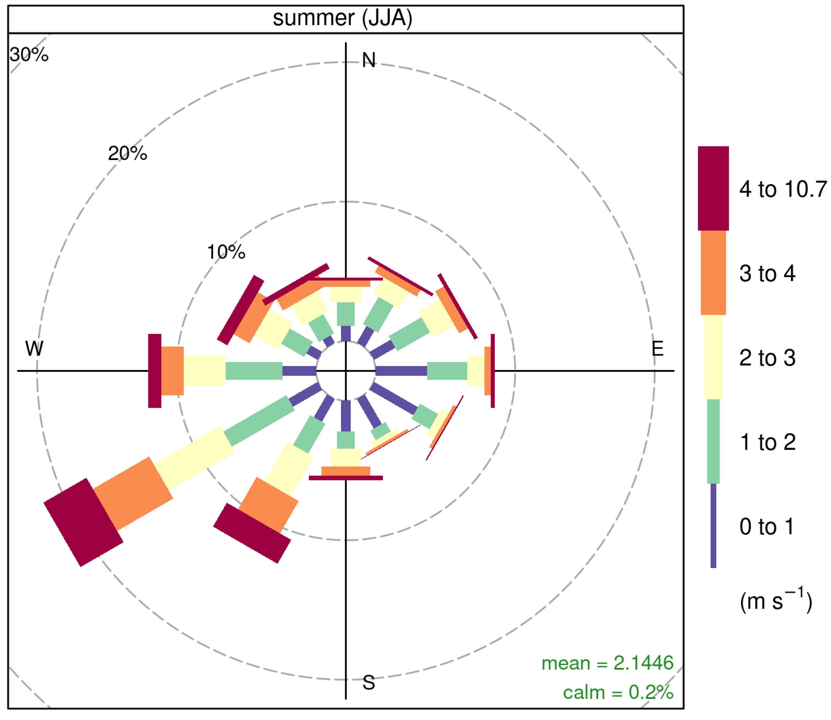
During the summer months, the dominant wind direction is southwest (240° N). Maximum wind speeds of up to 10.7 m/s were reached, with an average of 2.1 m/s (Figure 2).
3.4. Fuels Prediction
3.4.1. Surface Fuels
To relate fuel models to spatially continuous surfaces, we used remote sensing data and machine learning frameworks. Field plot locations and their respective dominant tree species label served as training points for image classification. To delimit non-relevant (non-burnable) land cover types (water, agricultural area, urban area and bare ground), 79 training points were established manually with the support of high-resolution true-color imagery.
Predictor variables comprised 119 layers at 10 m resolution from active and passive air- and space-borne sensors (Table 1). After pairing training locations with predictor variables, a random forest classification model was trained [40]. The number of trees was held constant at the default of 500. Hyperparameter mtry (number of candidates per split) was tuned with odd-numbered values ranging between 2 and 11. Model training was integrated in a forward feature selection (FFS) process as proposed by Meyer et al. [41]. The model is built successively, starting with the best-performing pair of predictors and adding further ones as long as the performance measure improves. This way, the resulting model is as simple as possible, which is more desirable than having tens or hundreds of terms. The FFS model was optimized using the Kappa index. Overall accuracy (OA) and the class confusion matrix were further consulted for model evaluation.
If training points are clustered in space, a traditional random k-fold cross validation (CV) comes with caveats. Spatial auto-correlation may cause an overly optimistic view on model performance. In this case, however, field sampling locations were randomly distributed over a large part of the study area. This justifies the use of a simple 5-fold random CV, which was implemented in the FFS process.
As an additional criterion, the area of applicability (AOA) was computed for the final model. It aims at estimating the extent to which a prediction model and its CV error can be applied. The underlying dissimilarity index is calculated for each pixel based on its distance to the closest training point in the multidimensional predictor space [42]. Both FFS and AOA were computed using the CAST package [43], while individual model training was facilitated by caret [44].
Finally, the model prediction yielded a four-class raster dataset. A simple majority filter (3 × 3 moving window) was applied to smooth out minor classification errors and reduce their effect on subsequent fire spread simulations. Tree species classes were assigned corresponding fuel model parameters for fire behavior analysis. The remaining class represents all non-burnable land cover types and was thus not assigned any values relevant to fire behavior.
3.4.2. Crown Bulk Density
Plot-level CBD values computed via FuelCalc [20] were subsequently used as target variable in a regression analysis. The same set of 119 predictors was used. Circular field plots (10 m radius) partially covered 4–9 pixels (10 × 10 m) of the predictor data. Therefore, all concerned values were extracted and weighted by their share of the plot area covered. Data were split into training and validation sets in a 70 to 30 ratio. Three predictor variables derived from Sentinel-2 (; ) and ALS data () were excluded, due to their near-zero variance. The training data used in this analysis had 30 observations and 119 predictors, disqualifying them for ordinary least squares regression. Many predictors are strongly correlated. This constellation calls for a regularized regression model, which aims at making a biased estimate of regression parameters. Bias is thus traded for variance [45].
We selected a ridge regression model for this task. Its regularization parameter lambda is dependent on the dataset. Lambda was tuned using a grid of 100 values ranging from 0.1 to 100. CV yielded the optimal value by considering the root mean squared error (RMSE) as a criterion. Ridge regression analysis was facilitated by R-packages glmnet [46] and caret [44]. The training data were centered and scaled prior to model training. A 5-fold random CV was implemented for the same reason as described in the previous section. Test runs revealed a non-normal distribution of model residuals. Consequently, the target variable was transformed, using the logarithmic function. In an attempt to expand the number of training samples, 15 plots of the German National Forest Inventory were added. Their tree lists were supplemented with LiDAR-derived CH and CBH and processed in FuelCalc. Predictor variables were extracted in the same way as for the remaining training points.
3.5. Fire Behavior and Hazard Modeling
Next to fuel loadings and fuelbed depth, FBFMs further consist of several constants, such as the surface-area-to-volume ratio (SAV), moisture of extinction (MOE), and heat content [47]. Constants were selected in accordance with existing standard FBFMs [47,48]. All fuel models received 1, 10, and 100 h SAV constants of 5906, 4249, and 4593, respectively. MOE was set to 30% and heat content to 18,622 Kj/kg.
FlamMap is a quasi-empirical fire spread model, widely used among forest and fire managers in operational settings [2]. Its main requirement is the fire landscape data, which consist of three terrain variables (elevation, aspect, and slope), four forest structure variables (CH, CBH, CC, and CBD) and a surface fuel classification [49]. Additional controls, e.g., fuel moisture, wind, or temperature, can be defined. FlamMap’s objective is to calculate spatio-temporal fire behavior under a unique set of environmental conditions. This is especially interesting when assessing the effects of varying weather conditions, fuel properties, or fire-related forest management actions.
To evaluate fire hazard in the Haard under a variety of environmental conditions, we set up a grid of realistic scenarios. We selected two options each for the components of (i) fuel moisture, (ii) wind speed, and (iii) air temperature. This resulted in a total of eight individual scenarios (Table 2).
Like many other regions, Central Europe recently experienced extremely hot and dry summers. Extended heat waves and the absence of precipitation fostered an increased number of ignitions. Surface fuel moisture content dropped and caused higher rates of fire spread. To reflect variable moisture conditions and their effects on fire spread, Scott and Burgan [48] proposed a set of scenarios along with their standard FBFMs. Dead (D) and live (L) fuels can each be assigned four moisture levels, ranging from very low to low, moderate and high (1–4), which are expressed as representative moisture content values in percentage values. Dead fuel moisture scenarios are characterized for time-lag categories 1, 10 and 100 h and range from 3 to 14 percent. Live fuel moisture scenarios include values for herbaceous and woody fuels and range from 30 (fully cured) to 150 (fully green) percent. We selected fuel moisture scenarios D1L1 and D3L1, which should correspond to the effect of a longer and a shorter pre-fire drought period. Both are characterized by very low moisture levels for live herbaceous (30%) and live woody (60%) vegetation. However, they differ in dead fuel moisture levels for time-lag categories 1, 10, and 100 h with 3%, 4%, and 5%, and 9%, 10%, and 11%, respectively.
FlamMap uses either weather time series data or single value inputs for individual weather components. Wind speed and direction strongly affect fire initiation and spread [50]. Both can either be static inputs or may be adjusted dynamically using the WindNinja module [51]. This numerical micro-scale wind flow model is designed for fire modeling applications and simulates mechanical and thermal effects of terrain, vegetation, and air temperature on the flow. It scales down wind speed and direction to finer spatial resolutions.
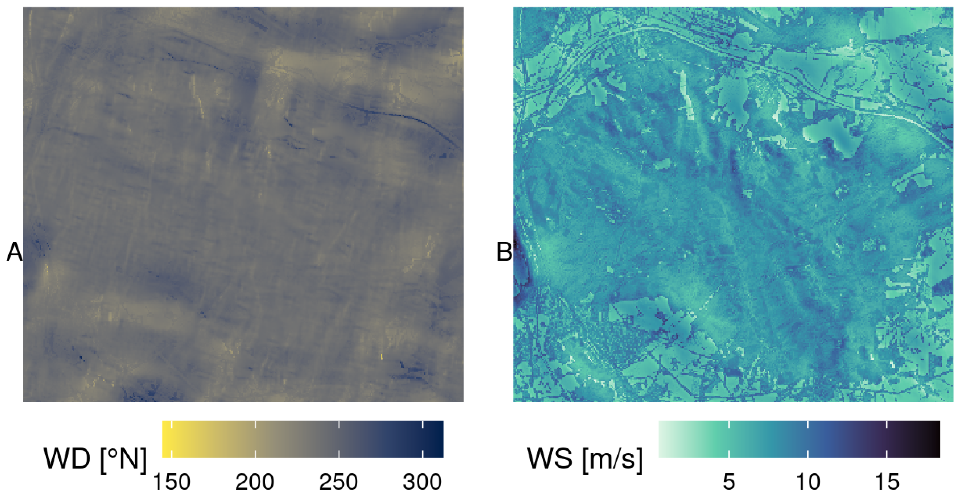
To investigate the impact of different weather conditions on fire hazard, we considered two values each for wind speed and air temperature. We compare peak (10 m/s) and average (2 m/s) wind speed as well as extreme (35 °C) and moderate (25 °C) summer temperatures. Figure 3 displays exemplary WindNinja outputs for the study area from constant wind speed (10 m/s) and direction (240° N). Despite revealing local anomalies, down-scaled wind characteristics remained similar to their original input constants for the most part.
The two most critical and valuable landscape fire behavior outputs for decision makers are fire intensity (expressed as FL) and the ROS [2]. Both are calculated on a pixel basis. Considered individually, both characteristics bear a limited hazard potential. Stationary high-intensity fires or fast-spreading low-intensity fires only pose minor challenges for containment efforts. However, quickly moving high-intensity fires are difficult to manage and contain, resulting in an elevated fire hazard potential.
In a second step, FlamMap employs the minimum travel time (MTT) algorithm to run fire spread simulations [52]. It requires a set of random or predefined ignition locations. Each fire burns under the same environmental conditions and stops after a specified duration. That makes MTT particularly useful for the analysis of effects of spatial patterns in fuels and topography [49]. Final perimeters are recorded for each simulated fire. Locations (pixels) that have burned more frequently throughout the simulation will receive higher conditional burn probabilities (CBP). This means they are more likely to burn in the case of a fire, but gives no indication of the probability of a fire starting. CBP values are scaled by their maximum and broken down into five ordinal classes, ranging from lowest to highest.
Next to CBP, MTT also produces a conditional flame length (CFL). It represents a weighted version of FL previously introduced in the context of landscape fire behavior. MTT distinguishes heading, flanking, and backing fire spread. Therefore, heading fire burns at a higher intensity than the other two. Throughout repeated fire spread simulations, every pixel can burn multiple times and with different intensities. MTT computes probabilities for 20 FL classes that sum up to 1. These are aggregated to a single value per pixel by applying probabilities as weights for the mid-point FL of each class (0.5, 1,..., 9.5, >9.5 m). The resulting CFL is considerably lower than FL from a landscape fire behavior calculation. Similar to CBP, CFL is subdivided into six standardized classes.
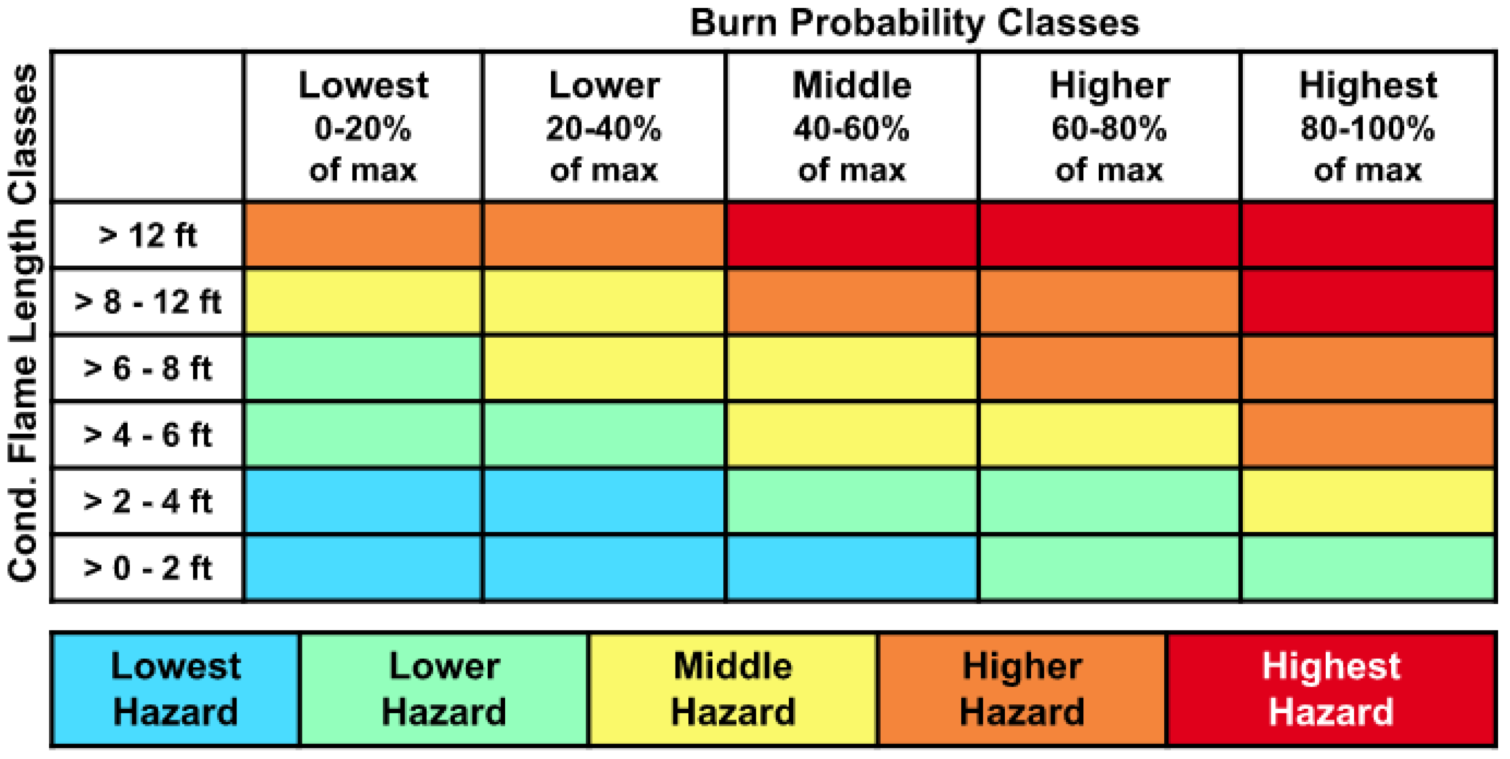
Integrated fire hazard (FH) is finally calculated from CFL and CBP, following the classification scheme proposed by the Interagency Fuels Treatment Decision Support System (IFTDSS) [53] (Figure 4). The scheme divides continuous fire behavior values into hazard categories, which are more intuitive to read. By combining both measures to a single metric, it offers a more holistic view on the present situation than other fire behavior variables.
A combination of high values in both categories leads to high FH, whereas high values in either one lead to medium FH at most. Equally to CBP, the five FH classes range from lowest to highest.
For each scenario, we ran fire spread simulations using the same set of 10,000 randomly distributed ignition locations. The maximum simulation time for MTT was set to 60 min. This constraint was selected to reflect a sensible reaction time for nearby fire departments. Local forest and fire management confirm that this value approximately matches reality. In addition to the non-burnable land cover class fire spread was restricted by barrier structures, such as major roads or water bodies surrounding the study area. These are represented by vector geometries, which serve as input data for the model.
4. Results
4.1. Surface Fuels
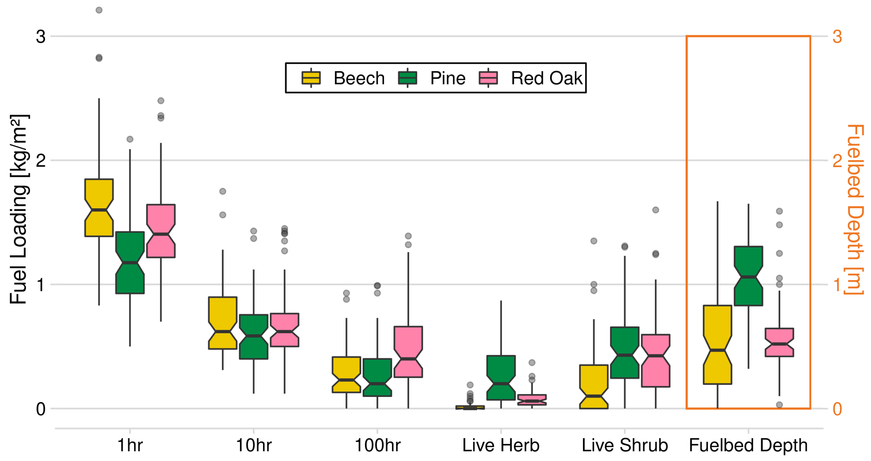
Field sampling yielded surface fuel loadings for three custom FBFMs. Distributions of sampling data are displayed in Figure 5. Custom FBFMs are created from the median of each parameter (see Table 3). Significant differences between all fuel models can be observed for 1 h fuels. They are generally greater than 1 h loadings of similar standard FBFMs suggested by [48]. In turn, 10 h fuels are very similar among all groups. Red oak shows significantly more 100 h fuels with approximately twice the loading of pine or beech. Pine has the largest quantities of live fuels, especially for herbaceous vegetation. Beech, however, forming dense top canopies and shading the forest ground well, only shows small live shrub loadings and almost no live herbs. This pattern is reflected in the fuelbed depth. Pine fuelbeds are about twice as deep as the others.
The FFS process found the best performing solution among 13,924 possible combinations of predictor variables. CV selected an optimal mtry of 2 and reported an OA of 0.971 with a Kappa of 0.967. The final model consisted of five variables, with being the most important one. and also scored high variable importance, followed by . Finally, was only able to add very little improvement to the model. FFS successfully reduced the number of predictors significantly (5 vs. 119) while keeping model performance high. For comparison, a classic random forest model was built, using all available predictors. Performance was still high, but both OA and Kappa decreased by 2.8% and 3.8%, respectively.
The model confusion matrix revealed a perfect classification of non-burnable areas. This may be explained by noticeable differences in the spectral signatures and vertical structure of non-burnable land cover (e.g., water bodies, urban area) compared to forest vegetation. Minor confusion was found between tree species classes. Errors ranged between 4% and 8%, with beech having slightly larger errors than pine and red oak. Previously separated validation samples (n = 90) were tested on the model prediction. All samples were classified correctly, yielding an OA and Kappa of 1.0. Overall, the fuel model classification results were very good. However, this could be expected, as it was a simple modeling task combined with a large range of powerful predictors.
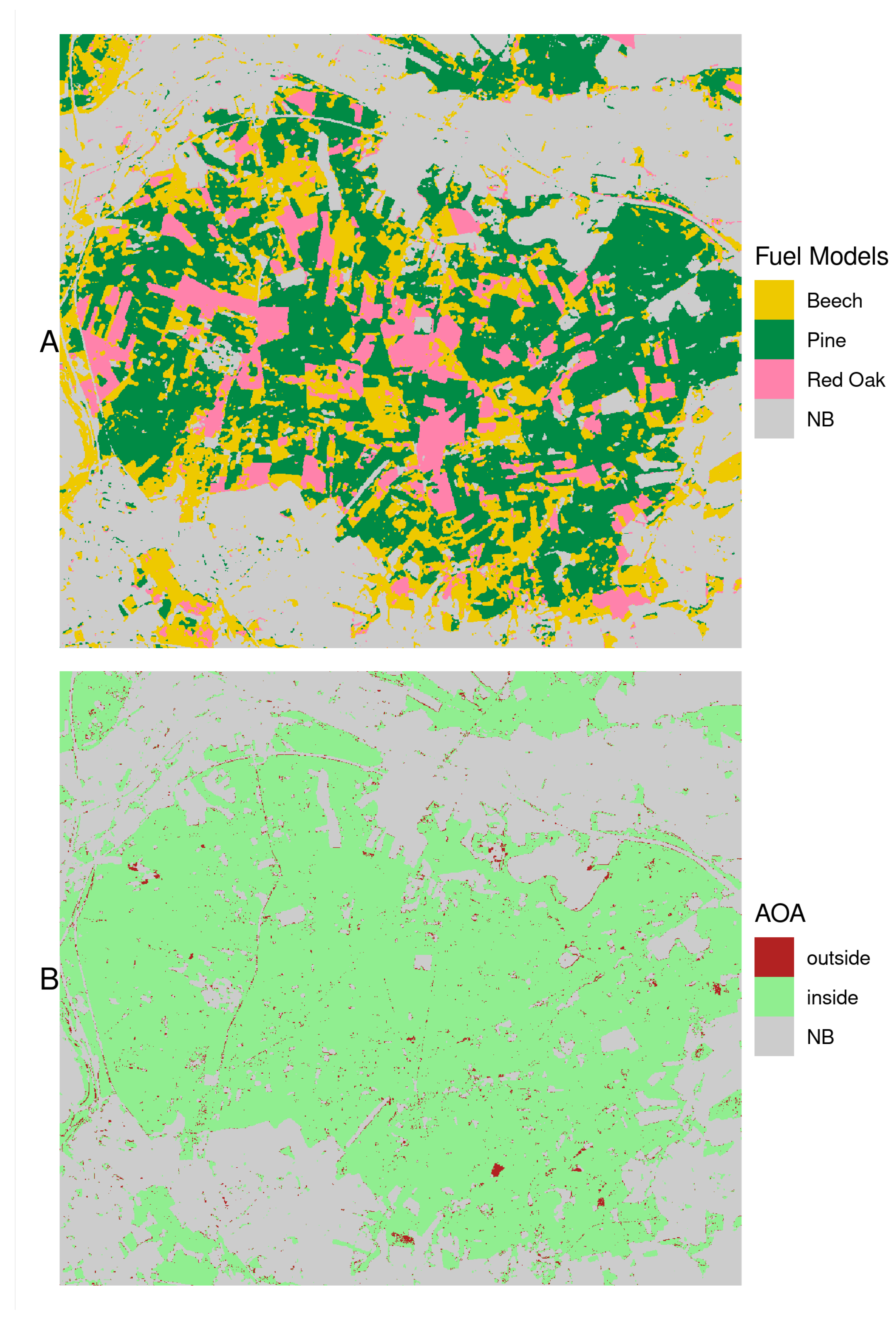
The final prediction is shown in Figure 6 alongside with the AOA. The dissimilarity of predictors from the training samples was only critical in areas less relevant for fire spread. Fewer than 1% of burnable pixels fell outside the AOA and represented mainly roads, bare ground or vegetation along water bodies. These areas are often located in close proximity to the forest edge or to existing fire barriers, which makes them less relevant for fire spread modeling.
4.2. Crown Bulk Density
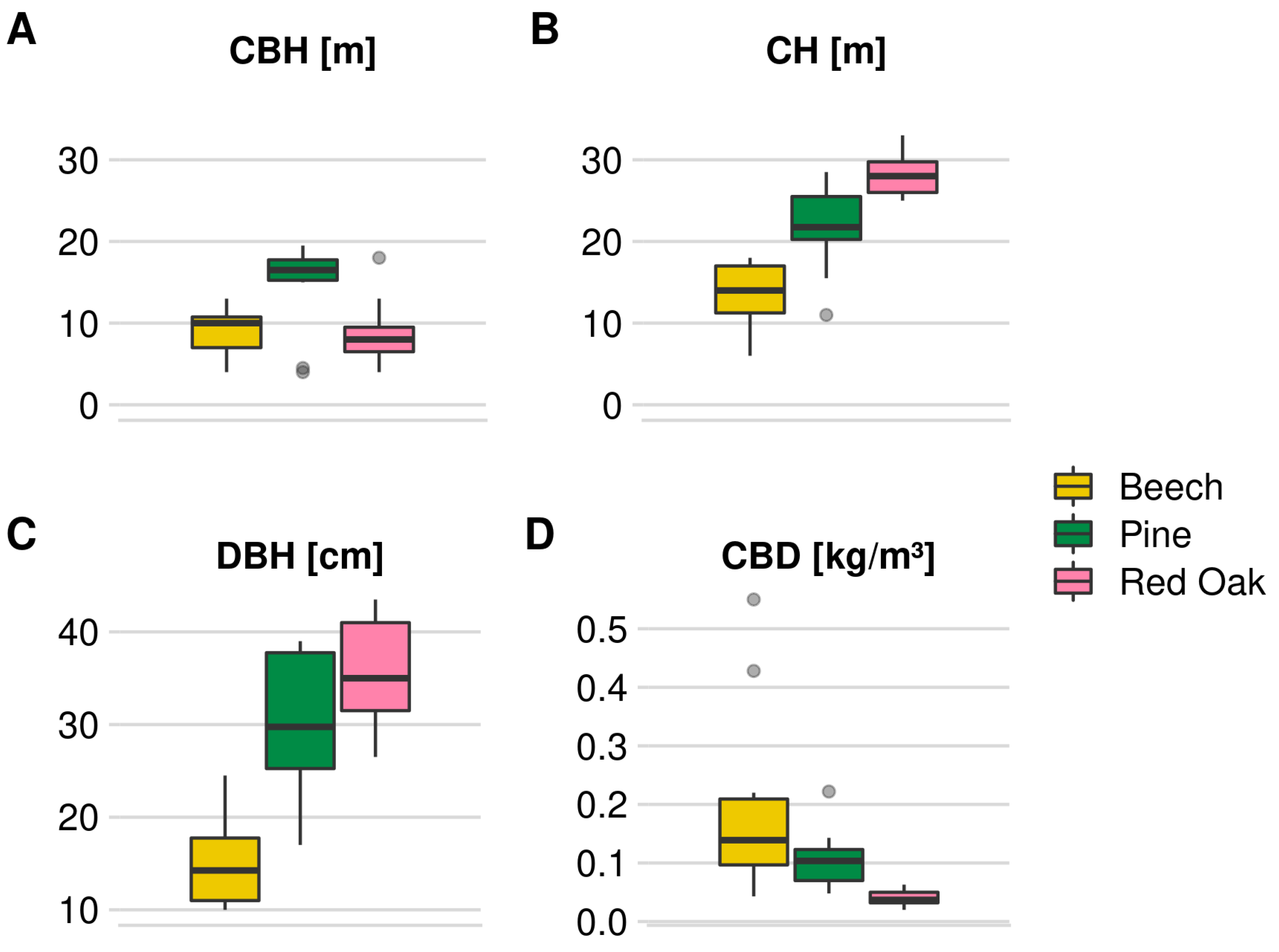
Field measurements of canopy fuel characteristics show clear differences between dominant species (see Figure 7). Many beech stands in the study area are young and have small DBH. They often occur in row-wise plantations with high stem density and nearly identical CBH and CH. Red oak and pine stands are older and less dense as a result of selective logging. Their DBH and CH are two to three times greater than those of beech. CBH, the height of the lowest live branch, is generally much lower for red oak compared to pine, while the opposite is the case for CH. As a consequence, the CBD estimates for red oak are lower.
Ridge regression analysis was applied to predict CBD for the Haard forest. CV selected an optimal regularization parameter lambda of 10.7. Overall, model performance was poor which was expected, considering the small number of training samples. A model-R2 of 0.59 with a RMSE of 0.054 was reported. Independent validation samples produced a higher R2 of 0.73, while RMSE degraded to 0.069. Although R2 is acceptable, RMSEs are large, considering a CBD training sample mean of 0.095. Differences in model performance and validation scores indicate the introduction of bias by ridge regression.
Variable importance scores indicated strong dependence on LiDAR-derived vertical structure metrics and optical predictor data. The most relevant predictors included , , , , , and . Further, the nine next relevant variables in the ranking, , , and , all describe vegetation structure in the upper third of the tree. This coincides with relative heights at which CBD can be found at the maximum.
We tested adding training samples from NFI plots (n = 15) but were not able to improve the model. On average, their derived CBD values were significantly smaller than the existing values based on field sampling. NFI surveys include records of species and CH among many other observations. However, they do not include CBH. Supplementing NFI tree lists, for example, with LiDAR-derived CBH at 10 m spatial resolution, is rather inaccurate, especially when considering plots with heterogeneous species composition, age, and vertical structure.
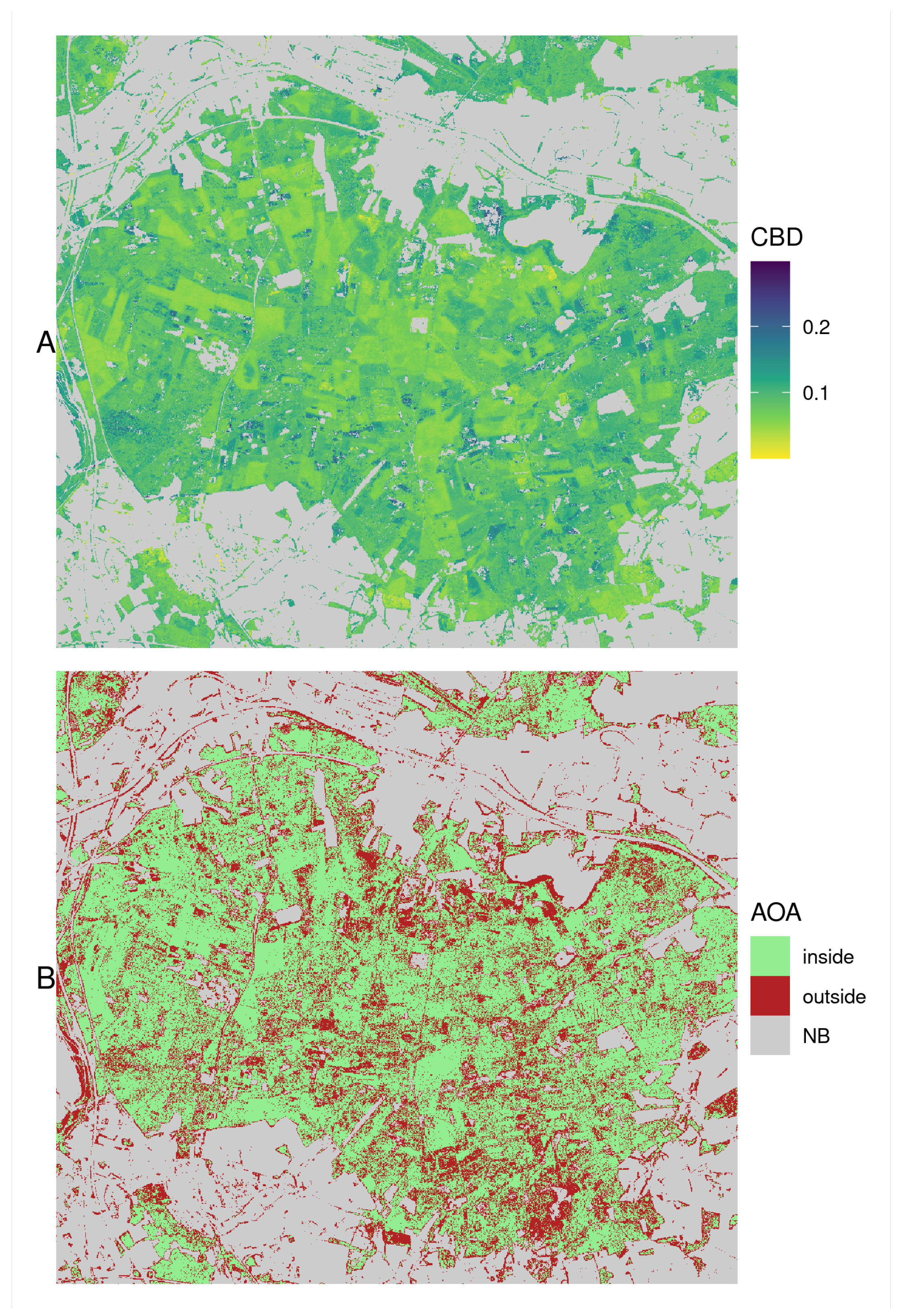
Spatial prediction and AOA for CBD are shown in Figure 8. CBD values range from 0 to 0.3. They roughly follow the tree species classification, while higher densities can be observed for pine than for beech and red oak. Anomalies in CBD within homogeneous patches dominated by a single species are related to structural differences. Considering only forested pixels, 20% fall outside the AOA. This may again be explained by the low number of training samples. A significant portion is located in areas with steeper slopes.
4.3. Fire Behavior and Hazard
Fire behavior was computed for the Haard forest considering landscape properties, fuel metrics, and eight sets of weather conditions. Variations in fire behavior can be observed in the spatial domain. This is related to the heterogeneity of surface fuels, vertical forest structure and terrain. Further, wind speed and fuel moisture impact fire behavior, resulting in major differences among scenarios. Air temperature, however, had no significant effect on fire behavior. Therefore, only scenarios S1, 3, 5, and 7 are evaluated in the following.
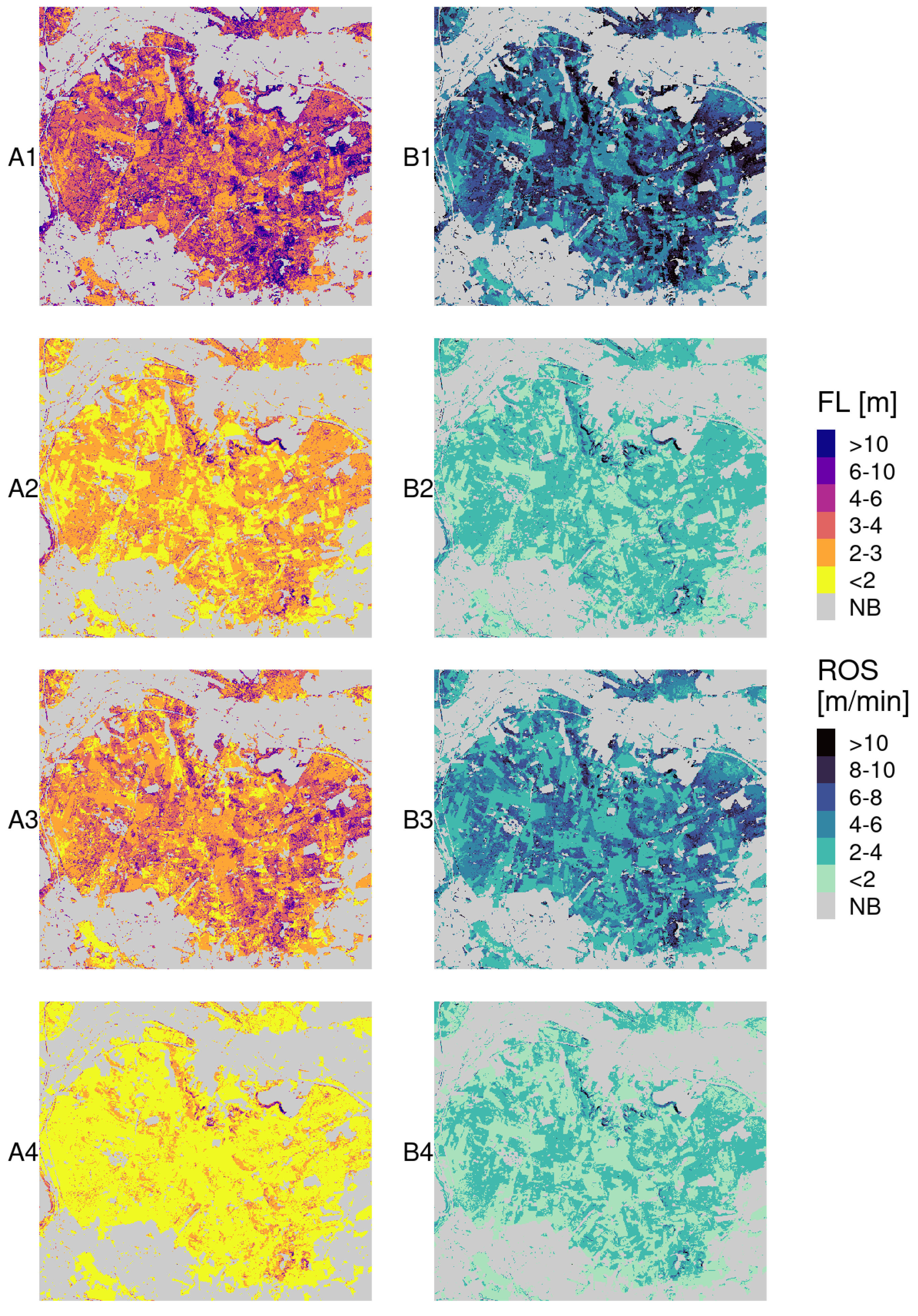
Overall, the strongest fire behavior was found for S1 (Figure 9 row 1). Low fuel moisture and high wind speed led to FL exclusively larger than 2 m, sporadically even exceeding 10 m. Low to medium FL predominantly occurred in red oak and beech stands. On the contrary, pine stands in particular showed high fire intensities. The same pattern was observed for ROS. Even more so than FL, ROS was closely linked to the spatial patterns of surface fuel models. Spread rates ranging from 6 to beyond 10 m/min were common in pine-dominated stands, whereas broad-leaved stands produced significantly slower fires. Most areas in the Haard with steep slopes are populated by pine. The combined effects of fire-prone pine fuel beds and steep slopes result in the highest observations of FL and ROS within the study area.
The effect of high wind speed on fire behavior becomes visible when comparing scenarios S1 with S3 (Figure 9 rows 1 and 2). Overall, a reduction in wind speed from 10 to 2 m/s cut the mean FL in half from 5.1 to 2.5 m, while ROS dropped from 6.8 to 2.6 m/min. Lower wind speed in S3 diminished fire behavior disproportionately in pine stands, which showed extremes in S1. A weaker, yet still significant, reduction occurred in beech and red oak stands. Few locations with high FL and ROS in the central northern and southwestern parts of the study area still stand out in S3 and S7 (Figure 9 rows 2 and 4). These correlate well with increased slopes and related higher wind speeds, highlighting their promoting effect on fire behavior.
Comparison of S1 and S5 (Figure 9 rows 1 and 3) emphasizes the influence of dead fuel moisture. S5 features similar spatial patterns in both FL and ROS, with extreme values consistently occurring in steep pine stands. On average, however, both are reduced significantly when facing increased dead fuel moisture levels. Mean FL dropped to 3.2 m while ROS slowed down to 4.8 m/min. Similar, yet weaker, shifts apply to average wind scenarios S3 and S7. Hence, a more substantial reduction in fire behavior was recorded for a decrease in wind speed as opposed to a decrease in dead fuel moisture.
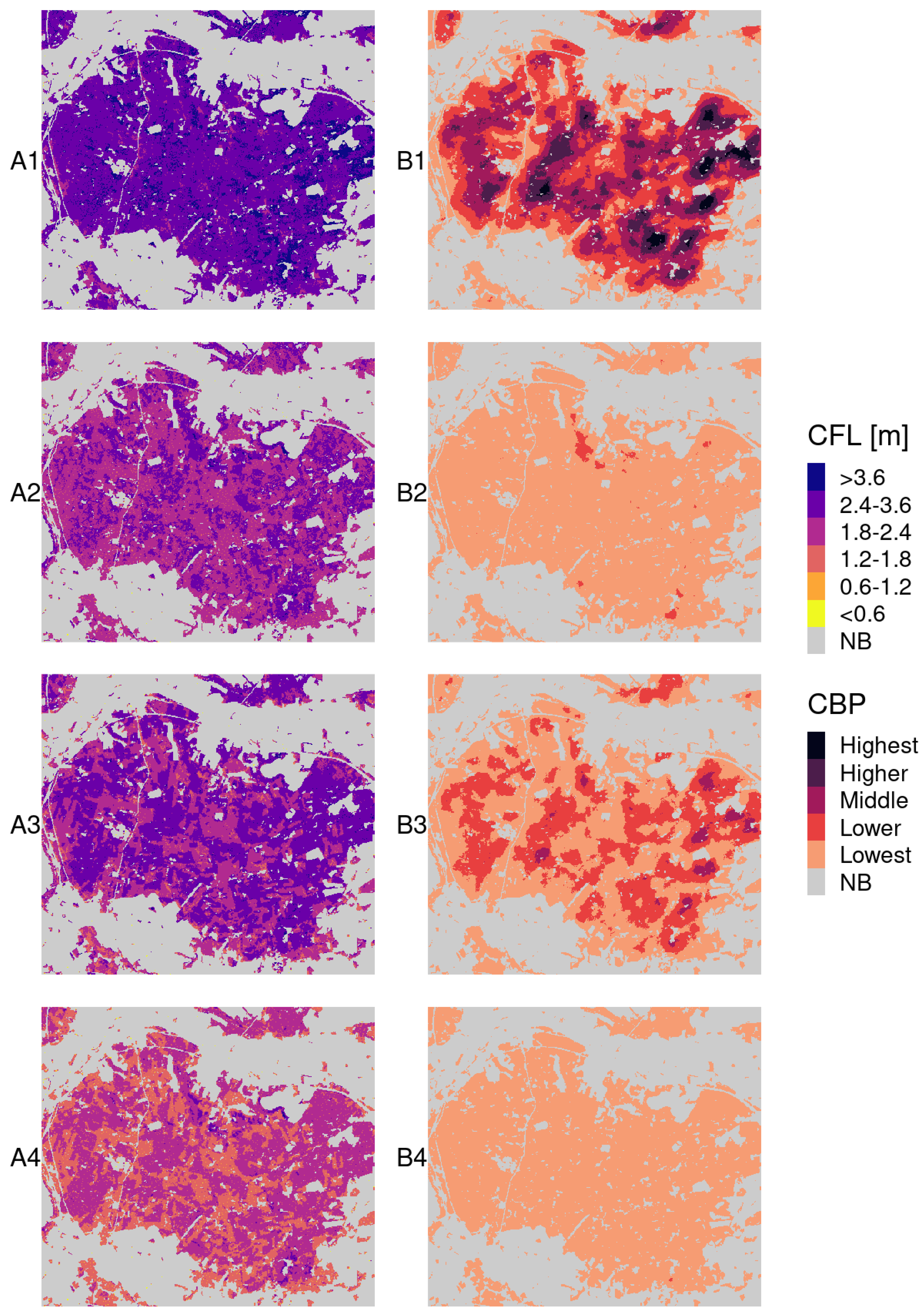
Fire behavior outputs from MTT fire spread simulations (Figure 10) show comparable patterns as landscape fire behavior results. While strong winds in S1 and S5 result in elevated CFL for the majority of the study area, average winds only lead to a few hotspots of small extent. CFL has substantially lower values than FL, which can be attributed to the weighted calculation method.
CBP for all scenarios was scaled, using the overall maximum of 0.013. Higher and highest CBP in S1 occurred in the center and the eastern part of the Haard. Both areas are characterized by large continuous pine stands indicating an interdependence. Within the limited simulation time, fire spread fastest and formed the largest perimeters when burning in this setting. Concerned locations consequently burned more frequently, leading to higher CBP. Increased fuel moisture content in S3 yielded similar spatial patterns, yet on a lower level without exceeding medium CBP. Disregarding few exceptions, S3 and S5 only produced CBP values belonging to the lowest category. This indicates that fire spread is very limited during the absence of strong winds. Even though spatial variations in CBP exist, they are hidden by the scaled classification scheme.
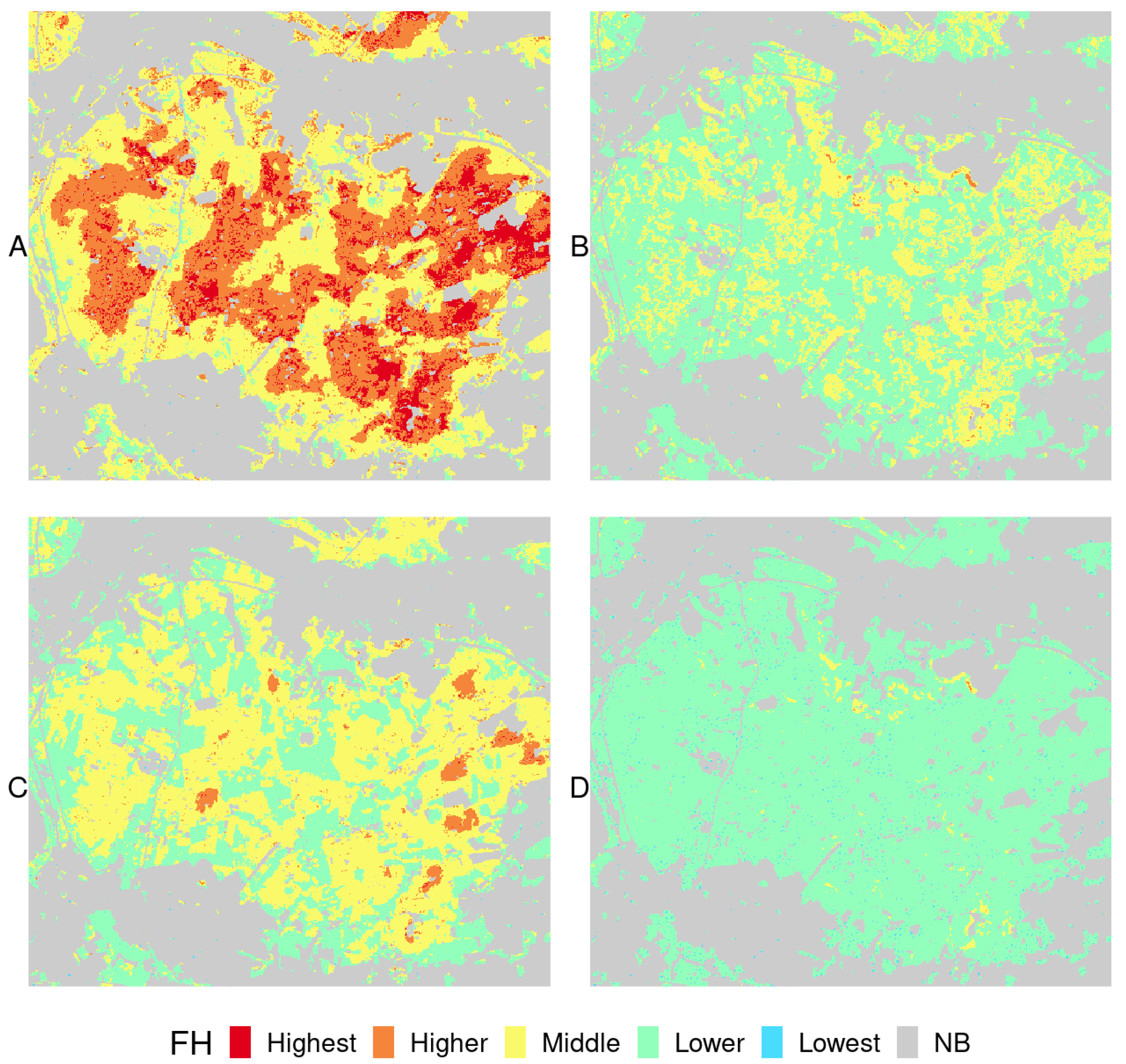
Similar to the fire behavior results, extreme FH only occurred during strong winds and with low fuel moisture present (Figure 11A). In case of a fire in these conditions, large pine stands in all parts of the study area appeared to be affected more severely than other species. Within pine stands, the highest FH category coincides with areas showing increased CBD or slopes. Regardless of fuel moisture, fire spread simulations featuring strong winds (Figure 11A,C) revealed a small number of FH hotspots.
Simulations for average wind scenarios S3 and S7 (Figure 11B,D) showed clearly reduced FH predictions. Low FH prevailed under both scenarios. While medium FH still emerged in pine-dominated areas for S3, it only sums up to a negligible extent in S7. It should be noted that in both cases, high FH can be found sporadically on steep slopes, despite the absence of strong winds.
5. Discussion
With this paper, we demonstrate a comprehensive workflow for the assessment of wildfire hazard in a small managed temperate forest. Surface and canopy fuels were sampled in field surveys and extrapolated in space, using predictive statistical modeling methods. We combined fuel information with other variables, completing the fire landscape to feed fire behavior models, simulate the growth of several thousands fires, and derive a hazard index.
Spatial predictions of fuel characteristics were performed based on field data and statistical modeling. Sufficient training data in combination with powerful predictor variables led to a near-perfect classification result for three surface fuel models. Dense ALS point clouds allowed for directly deriving canopy fuel metrics, such as CC, CH, and CBH, due to their relatively low measurement error.
CBD, on the contrary, required regression analysis using training data from field observations. This canopy fuel variable could not be measured directly but was estimated via allometric equations, using field measurements of other tree properties. Estimates then represented the reference for statistical modeling. Through this process, training data were subject to multiple sources of errors. Due to the limited number of samples, the resulting statistical model was weak. The value ranges of field and predicted CBD were similar to previous studies by Andersen et al. [29] and Erdody and Moskal [21]. Their regression model validation produced RMSEs of 0.27 (R2 = 0.84) and 0.024 (R2 = 0.88) while including 101 and 57 field sampling locations, respectively. Cameron et al. [30] reported a RMSE of 0.098 (R2 = 0.78) whilst using 52 training samples. Considering the low number of samples in the present study, a RMSE of 0.069 (R2 = 0.73) was acceptable, especially as CBD is only one of multiple components of the FH assessment. Further, predicted CBD showed variations between stands with different dominant species, which is comprehensible from an ecological stand point. The ridge regression model introduced bias in exchange for reducing variance. This effect may have been reduced by applying a more complex tuning approach, such as nested cross validation. Alternatively, a better fit may be achieved through more flexibility, for example, by applying a penalized generalized additive model.
Errors in the prediction of all fuel variables may have been caused by the temporal gap between field (summers 2019 and 2021) and LiDAR (winter 2020) data acquisition. In addition, the collection of LiDAR data over deciduous trees during their defoliated phase is problematic. This may cause underestimation of CC and other metrics involving the number of canopy returns.
LiDAR-based predictor variables were crucial for modeling CBD and could contribute to the mapping of surface fuel models. Sentinel-2 data were able to support both efforts. In particular, bands 4, 5, and 6, and the NDVI were listed among the most important predictors. All involve wavelengths in the near-infrared, which are proven to describe vegetation characteristics. Temporal composites of the 10th and 90th percentiles were more important than the ones of the 50th percentile. They represent stages of the vegetative cycle, which reveal more differences among tree species than the annual median. The surface fuel classification model, for instance, took advantage of these differences by selecting and as two of its five predictors. Sentinel-1, on the contrary, did not play a relevant role. The SAR signal is able to partially penetrate the forest canopy and was expected to react to differences in CBD. Theses differences may have been too subtle to be captured, or were explained more precisely by other predictors.
As Papadopoulos and Pavlidou [50] stated, fire behavior and spread models require major assumptions, and their output accuracy heavily depends on the quality of input data. This study classified three FBFMs, each connected to one dominant tree species. Within stands, however, the species composition may slightly differ from observations made at sampling locations, altering surface fuel properties. Additional uncertainty in FH prediction arises from the accumulation of errors over the course of a fire growth simulation and the common problem of an unfeasible validation against real wildfire events [50]. Despite numerous sources of uncertainty, simulation-based FH is more robust and informative than simple fire behavior calculations, as it considers flanking and backing fire, not only heading fire [54]. CBP (and therein FH) gives no indication about the probability of a fire starting. As most fires are caused by humans, ignition density is likely to increase with proximity to man-made structures, such as roads, paths or recreational points of interest. Together with an accessibility assessment for fire suppression units, this information should be considered in any follow-up risk assessment.
The present analysis revealed wind speed and slope to be the most relevant factors of FH in the Haard forest. Further, low fuel moisture content can amplify FH. While high wind speed and low fuel moisture are difficult to prevent, forest management can address elevated FH on slopes. These areas could be converted to stands with low stem density, consisting of species that produce slow and weakly burning surface fuels (e.g., red oak). The same strategy could be applied to areas surrounding medical or recreational facilities, as they bear elevated risk. Other FH hotspots were identified in large pine stands. Among the three dominant species in the study area, pine’s fuel bed produced the highest flame lengths and spread rates. Additionally, fires reached their largest perimeters in pine-dominated areas, resulting in the highest values for CBP. This may, in part, be related to the fact that local pine stands are larger and more contiguous than beech and oak stands, allowing fire to cover longer distances through a homogeneous and highly flammable landscape. To mitigate fire spread in large pine stands, species composition and forest structure could be diversified, creating a more heterogeneous landscape. Fire barriers in the form of planted strips of broadleaved species could be introduced perpendicular to the dominant wind direction. The Haard is confined by roads and water bodies in the west and north. However, wind and, with it, fire predominantly move toward the east. FH calculations for high wind speeds suggest a need to secure the eastern forest edge to prevent potential wildfire from affecting adjacent campsites and agriculture.
Future research in Central Europe could aim at developing detailed fuels datasets with national or continental extents. These are needed to allow for wildfire hazard and risk assessments on various spatial scales. Previous studies as well as the present one have confirmed the importance of LiDAR data for the spatial prediction of wildfire fuels. ALS data, however, have high acquisition costs and are rarely accessible. Two current trends in LiDAR remote sensing may advance the quantification of fuel variables in the near future. The growing availability of drones with lightweight laser scanning instruments enables high temporal and spatial resolution in small areas. From a global perspective, space-borne LiDAR missions, such as GEDI, will improve not only biomass and CH mapping, but also CBH or CBD estimation.
6. Conclusions
We characterized the fire landscape in a small managed temperate forest by connecting field and remote sensing data. With this baseline, we calculated fire behavior, simulated fire spread and deduced spatial wildfire hazard information. By interpreting the results of this process, we identified critical areas that should receive special attention in management actions related to wildfire safety. With fire as an emerging threat to Central European forests, interest in such information may grow. We deliberately used openly accessible data and low-cost instruments for field sampling. Processing was facilitated through freely available software without advanced computational requirements. These attributes lower the hurdle for forest management to obtain FH information, following our approach.
Author Contributions
Conceptualization, methodology, data curation, formal analysis, validation, visualization, writing—original draft preparation, project administration, J.H.; investigation, J.H. and E.O.; writing—review and editing, J.H., E.O. and E.P.; supervision, E.P. All authors have read and agreed to the published version of the manuscript.
Funding
This research received no external funding.
Institutional Review Board Statement
Not applicable.
Informed Consent Statement
Not applicable.
Data Availability Statement
Data, code, and instructions on how to reproduce this study can be accessed via https://github.com/joheisig/Haard_Wildfire_Fuels_Hazard (27 January 2022).
Acknowledgments
We thank Harald Klingebiel at RWR Ruhr Grün for sharing his experience on fire behavior and history in the Haard. Further, we are grateful to Gregory Dillon, Duncan Lutes and Charles McHugh at the Missoula Fire Sciences Laboratory for their valuable advice on fire and fuels modeling. Thanks also goes to Lukas Blickensdörfer at the Thünen Institute for his help with forest inventory data. We acknowledge support from the Open Access Publication Fund of the University of Münster.
Conflicts of Interest
The authors declare no conflict of interest.
References
- IPCC. Climate Change 2014: Synthesis Report. In Contribution of Working Groups I, II and III to the Fifth Assessment Report of the Intergovernmental Panel on Climate Change; Core Writing Team, Pachauri, R.K., Meyer, L.A., Eds.; Technical Report; IPCC: Geneva, Switzerland, 2014; p. 151. [Google Scholar]
- Cardil, A.; Monedero, S.; Schag, G.; de Miguel, S.; Tapia, M.; Stoof, C.R.; Silva, C.A.; Mohan, M.; Cardil, A.; Ramirez, J. Fire behavior modeling for operational decision-making. Curr. Opin. Environ. Sci. Health 2021, 23, 100291. [Google Scholar] [CrossRef]
- Schuldt, B.; Buras, A.; Arend, M.; Vitasse, Y.; Beierkuhnlein, C.; Damm, A.; Gharun, M.; Grams, T.E.; Hauck, M.; Hajek, P.; et al. A first assessment of the impact of the extreme 2018 summer drought on Central European forests. Basic Appl. Ecol. 2020, 45, 86–103. [Google Scholar] [CrossRef]
- BMEL. Deutschlands Wald im Klimawandel-Eckpunkte und Maßnahmen; Technical Report; Bundesministerium für Ernährung und Landwirtschaft: Bonn, Germany, 2019.
- BMEL. Waldbrandstatistik der Bundesrepublik Deutschland für das Jahr 2019; Technical Report; Bundesministerium für Ernährung und Landwirtschaft: Bonn, Germany, 2019.
- Dillon, G.; Menakis, J.; Fay, F. Wildland Fire Potential: A Tool for Assessing Wildfire Risk and Fuels Management Needs. In Proceedings of the Large Wildland Fires Conference; U.S. Department of Agriculture, Forest Service, Rocky Mountain Research Station: Missoula, MT, USA, 2015; pp. 60–76. [Google Scholar]
- Keane, R.E.; Burgan, R.; van Wagtendonk, J. Mapping wildland fuels for fire management across multiple scales: Integrating remote sensing, GIS, and biophysical modeling. Int. J. Wildland Fire 2001, 10, 301. [Google Scholar] [CrossRef]
- Keane, R.E.; Gray, K.; Bacciu, V. Spatial Variability of Wildland Fuel Characteristics in Northern Rocky Mountain Ecosystems; Technical Report RMRS-RP-98; U.S. Department of Agriculture, Forest Service, Rocky Mountain Research Station: Ft. Collins, CO, USA, 2012. [CrossRef] [Green Version]
- Chuvieco, E.; Aguado, I.; Salas, J.; García, M.; Yebra, M.; Oliva, P. Satellite Remote Sensing Contributions to Wildland Fire Science and Management. Curr. For. Rep. 2020, 6, 81–96. [Google Scholar] [CrossRef]
- White, J.C.; Tompalski, P.; Vastaranta, M.; Wulder, M.A.; Saarinen, N.; Stepper, C.; Coops, N.C. A Model Development and Application Guide for Generating an Enhanced Forest Inventory Using Airborne Laser Scanning Data and an Area-Based Approach; Technical Report; Natural Resources Canada, Canadian Wood Fibre Center: Ottawa, ON, Canada, 2017. [Google Scholar]
- Finney, M.A.; McHugh, C.W.; Grenfell, I.C.; Riley, K.L.; Short, K. A simulation of probabilistic wildfire risk components for the continental United States. Stoch. Environ. Res. Risk Assess. 2011, 25, 973–1000. [Google Scholar] [CrossRef] [Green Version]
- Oliveira, S.; Rocha, J.; Sá, A. Wildfire risk modeling. Curr. Opin. Environ. Sci. Health 2021, 23, 100274. [Google Scholar] [CrossRef]
- Botequim, B.; Fernandes, P.M.; Garcia-Gonzalo, J.; Silva, A. Coupling fire behaviour modelling and stand characteristics to assess and mitigate fire hazard in a maritime pine landscape in Portugal. Eur. J. Forest Res. 2017, 136, 527–542. [Google Scholar] [CrossRef]
- Taccaliti, F.; Venturini, L.; Marchi, N.; Lingua, E. Forest fuel assessment by LiDAR data. A case study in NE Italy. In Proceedings of the 23rd EGU General Assembly, Online, 19–30 April 2021. [Google Scholar] [CrossRef]
- Stockdale, C.; Barber, Q.; Saxena, A.; Parisien, M.A. Examining management scenarios to mitigate wildfire hazard to caribou conservation projects using burn probability modeling. J. Environ. Manag. 2019, 233, 238–248. [Google Scholar] [CrossRef]
- Lutes, D.C.; Keane, R.E. Fuel Load (FL). In FIREMON: Fire Effects Monitoring and Inventory System; Lutes, D.C., Keane, R.E., Caratti, J.F., Key, C.H., Benson, N.C., Sunderland, S., Gangi, L., Eds.; Gen. Tech. Rep. RMRS-GTR-164-CD; U.S. Department of Agriculture, Forest Service, Rocky Mountain Research Station: Fort Collins, CO, USA, 2006; pp. 1–25. [Google Scholar]
- Brown, J.K. Handbook for Inventorying Downed Woody Material; Technical Report; U.S. Department of Agriculture, Forest Service, Intermountain Forest and Range Experiment Station: Ogden, UT, USA, 1974. [Google Scholar]
- Keane, R.E.; Reinhardt, E.D.; Scott, J.; Gray, K.; Reardon, J. Estimating forest canopy bulk density using six indirect methods. Can. J. For. Res. 2005, 35, 724–739. [Google Scholar] [CrossRef]
- Lutes, D.C. FuelCalc User’s Guide (Version 1.7); U.S. Department of Agriculture, Forest Service, Rocky Mountain Research Station: Missoula, MT, USA, 2021.
- Reinhardt, E.; Lutes, D.C.; Scott, J.H. FuelCalc: A Method for Estimating Fuel Characteristics. In Proceedings of the Fuels Management-How to Measure Success: Conference Proceedings, Portland, OR, USA, 28–30 March 2006; p. 10. [Google Scholar]
- Erdody, T.L.; Moskal, L.M. Fusion of LiDAR and imagery for estimating forest canopy fuels. Remote Sens. Environ. 2010, 114, 725–737. [Google Scholar] [CrossRef]
- Scott, J.H.; Reinhardt, E.D. Estimating canopy fuels in conifer forests. Fire Manag. Today 2002, 62, 6. [Google Scholar]
- Gorelick, N.; Hancher, M.; Dixon, M.; Ilyushchenko, S.; Thau, D.; Moore, R. Google Earth Engine: Planetary-scale geospatial analysis for everyone. Remote Sens. Environ. 2017, 202, 18–27. [Google Scholar] [CrossRef]
- Mullissa, A.; Vollrath, A.; Odongo-Braun, C.; Slagter, B.; Balling, J.; Gou, Y.; Gorelick, N.; Reiche, J. Sentinel-1 SAR Backscatter Analysis Ready Data Preparation in Google Earth Engine. Remote Sens. 2021, 13, 1954. [Google Scholar] [CrossRef]
- Bezirksregierung Köln. Nutzerinformationen für Die 3D-Messdaten aus dem Laserscanning für NRW. 2020. Available online: https://www.bezreg-koeln.nrw.de/brk_internet/geobasis/hoehenmodelle/nutzerinformationen.pdf (accessed on 27 January 2022).
- R Core Team. R: A Language and Environment for Statistical Computing; R Foundation for Statistical Computing: Vienna, Austria, 2021. [Google Scholar]
- Roussel, J.R.; Auty, D.; Coops, N.C.; Tompalski, P.; Goodbody, T.R.; Meador, A.S.; Bourdon, J.F.; de Boissieu, F.; Achim, A. lidR: An R package for analysis of Airborne Laser Scanning (ALS) data. Remote Sens. Environ. 2020, 251, 112061. [Google Scholar] [CrossRef]
- Hijmans, R.J. Terra: Spatial Data Analysis. R Package Version 1.3-22. 2021. Available online: https://CRAN.R-project.org/package=terra (accessed on 27 January 2022).
- Andersen, H.E.; McGaughey, R.J.; Reutebuch, S.E. Estimating forest canopy fuel parameters using LIDAR data. Remote Sens. Environ. 2005, 94, 441–449. [Google Scholar] [CrossRef]
- Cameron, H.A.; Schroeder, D.; Beverly, J.L. Predicting black spruce fuel characteristics with Airborne Laser Scanning (ALS). Int. J. Wildland Fire, 2021; in press. [Google Scholar] [CrossRef]
- Chamberlain, C.P.; Sánchez Meador, A.J.; Thode, A.E. Airborne lidar provides reliable estimates of canopy base height and canopy bulk density in southwestern ponderosa pine forests. For. Ecol. Manag. 2021, 481, 118695. [Google Scholar] [CrossRef]
- Chuvieco, E.; Riaño, D.; Van Wagtendok, J.; Morsdof, F. Fuel Loads and Fuel Type Mapping. In Wildland Fire Danger Estimation and Mapping—The Role of Remote Sensing; World Scientific Publishing Co. Pte. Ltd.: Singapore, 2003; Volume 4, pp. 119–142. [Google Scholar] [CrossRef]
- Khosravipour, A.; Skidmore, A.K.; Isenburg, M.; Wang, T.; Hussin, Y.A. Generating Pit-free Canopy Height Models from Airborne Lidar. Photogramm. Eng. Remote Sens. 2014, 80, 863–872. [Google Scholar] [CrossRef]
- Riaño, D. Modeling airborne laser scanning data for the spatial generation of critical forest parameters in fire behavior modeling. Remote Sens. Environ. 2003, 86, 177–186. [Google Scholar] [CrossRef]
- Novo, A.; Fariñas-Álvarez, N.; Martínez-Sánchez, J.; González-Jorge, H.; Fernández-Alonso, J.M.; Lorenzo, H. Mapping Forest Fire Risk—A Case Study in Galicia (Spain). Remote Sens. 2020, 12, 3705. [Google Scholar] [CrossRef]
- Parker, G.G.; Harmon, M.E.; Lefsky, M.A.; Chen, J.; Pelt, R.V.; Weis, S.B.; Thomas, S.C.; Winner, W.E.; Shaw, D.C.; Frankling, J.F. Three-dimensional Structure of an Old-growth Pseudotsuga-Tsuga Canopy and Its Implications for Radiation Balance, Microclimate, and Gas Exchange. Ecosystems 2004, 7, 440–453. [Google Scholar] [CrossRef]
- Aber, J.D. Foliage-Height Profiles and Succession in Northern Hardwood Forests. Ecology 1979, 60, 18–23. [Google Scholar] [CrossRef]
- Rouse, J.; Hass, R.; Schell, J.; Deering, D. Monitoring vegetation systems in the great plains with ERTS. Third Earth Resour. Technol. Satell. Symp. 1973, 1, 309–317. [Google Scholar]
- Boessenkool, B. rdwd: Select and Download Climate Data from ’DWD’ (German Weather Service). R Package Version 1.5.0. 2021. Available online: https://CRAN.R-project.org/package=rdwd (accessed on 27 January 2022).
- Breiman, L. Random Forests. Mach. Learn. 2001, 45, 5–32. [Google Scholar] [CrossRef] [Green Version]
- Meyer, H.; Reudenbach, C.; Hengl, T.; Katurji, M.; Nauss, T. Improving performance of spatio-temporal machine learning models using forward feature selection and target-oriented validation. Environ. Model. Softw. 2018, 101, 1–9. [Google Scholar] [CrossRef]
- Meyer, H.; Pebesma, E. Predicting into unknown space? Estimating the area of applicability of spatial prediction models. Methods Ecol. Evol. 2021, 12, 1620–1633. [Google Scholar] [CrossRef]
- Meyer, H. CAST: `caret’ Applications for Spatial-Temporal Models. R Package Version 0.5.1. 2021. Available online: https://CRAN.R-project.org/package=CAST (accessed on 27 January 2022).
- Kuhn, M. caret: Classification and Regression Training. R Package Version 6.0-88. 2021. Available online: https://CRAN.R-project.org/package=caret (accessed on 27 January 2022).
- James, G.; Witten, D.; Hastie, T.; Tibshirani, R. (Eds.) An Introduction to Statistical Learning: With Applications in R; Number 103 in Springer Texts in Statistics; Springer: New York, NY, USA, 2013. [Google Scholar]
- Friedman, J.; Hastie, T.; Tibshirani, R. Regularization Paths for Generalized Linear Models via Coordinate Descent. J. Stat. Softw. 2010, 33, 1–22. [Google Scholar] [CrossRef] [Green Version]
- Anderson, H.E. Aids to Determining Fuel Models for Estimating Fire Behavior; Technical Report INT-GTR-122; U.S. Department of Agriculture, Forest Service, Intermountain Forest and Range Experiment Station: Ogden, UT, USA, 1982. [Google Scholar] [CrossRef] [Green Version]
- Scott, J.H.; Burgan, R.E. Standard Fire Behavior Fuel Models: A Comprehensive Set for Use with Rothermel’s Surface Fire Spread Model; Technical Report RMRS-GTR-153; U.S. Department of Agriculture, Forest Service, Rocky Mountain Research Station: Ft. Collins, CO, USA, 2005. [Google Scholar]
- Finney, M.A. An overview of FlamMap fire modeling capabilities. In Proceedings of the Fuels Management-How to Measure Success: Conference Proceedings, Proceedings RMRS-P-41, Portland, OR, USA, 28–30 March 2006; Andrews Patricia, L., Butler Bret, W., Eds.; US Department of Agriculture, Forest Service, Rocky Mountain Research Station: Fort Collins, CO, USA, 2006; Volume 41, pp. 213–220. [Google Scholar]
- Papadopoulos, G.D.; Pavlidou, F.N. A Comparative Review on Wildfire Simulators. IEEE Syst. J. 2011, 5, 233–243. [Google Scholar] [CrossRef]
- Forthofer, J.M.; Butler, B.W.; Wagenbrenner, N.S. A comparison of three approaches for simulating fine-scale surface winds in support of wildland fire management. Part I. Model formulation and comparison against measurements. Int. J. Wildland Fire 2014, 23, 969. [Google Scholar] [CrossRef]
- Finney, M.A. Fire growth using minimum travel time methods. Can. J. For. Res. 2002, 32, 1420–1424. [Google Scholar] [CrossRef]
- US Department of the Interior & US Department of Agriculture. Interagency Fuels Treatment Decision Support System (IFTDSS) (Version 3.4.1.3). 2021. Available online: https://iftdss.firenet.gov/ (accessed on 27 January 2022).
- Calkin, D.E.; Ager, A.A.; Gilbertson-Day, J. Wildfire Risk and Hazard: Procedures for the First Approximation; Technical Report RMRS-GTR-235; U.S. Department of Agriculture, Forest Service, Rocky Mountain Research Station: Ft. Collins, CO, USA, 2010. [Google Scholar] [CrossRef] [Green Version]
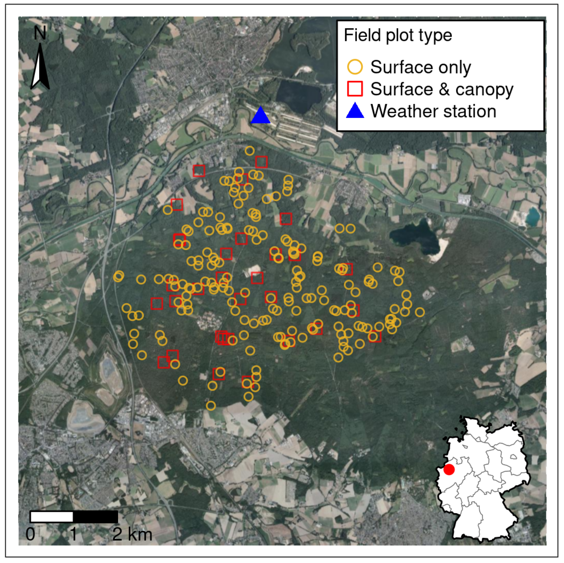
Figure 1.
Our study area is a managed temperate forest dominated by Scots pine, read oak and European beech. Located at 51.7° N, 7.2° E (red dot) in densely populated North Rhine-Westphalia, Germany, it is surrounded by agriculture and industry, serving as a local recreation area. The map displays 215 surface fuel sampling locations, of which 30 were used to additionally sample canopy fuel characteristics. Wind properties were assessed at a nearby weather station.

Figure 2.
Wind direction and speed aggregated from hourly data in close proximity to the study area during months June, July, and August and from 2000 to 2021. The dominant wind direction was identified as southwest (240° N). Average wind speed is 2.1 m/s, whereas a maximum speed of 10.7 m/s was recorded.

Figure 3.
Wind direction (WD; (A)) in degrees north and wind speed (WS; (B)) in meters per second down-scaled and adjusted to the study area’s terrain using WindNinja software. Constant input values were assessed in an exploratory analysis of weather station data. WD was fixed at 240° N, WS at 10 m/s.

Figure 4.
Integrated fire hazard (FH) classification scheme proposed by the Interagency Fuels Treatment Decision Support System (IFTDSS) [53]. It categorizes continuous fire behavior variables (CFL and CBP) to present a single intuitive metric. The highest FH is only reached in places where both CFL and CBP are very high.

Figure 5.
Boxplot of sampled surface fuel parameters for each fuel model. Dead and live fuel loadings are measured in [kg/m2], height of the fuelbed is in [m]. Beech and red oak produce slightly more 1 and 100 h fuels, while more live herbaceous biomass is found in pine stands. Higher-growing live fuels cause pine’s fuelbed depth to exceed that of the others.

Figure 6.
Surface fuel model prediction (A) and respective area of applicability (AOA; (B)). Spatial patterns originating from forest management are clearly visible. Pine is the most abundant species in the study area (51%) followed by beech (32%) and red oak (17%). Burnable pixels falling outside the AOA sum up to less than 1%.

Figure 7.
Boxplot of canopy fuel parameters from field sampling for each fuel model. Parameters include crown base height (CBH; (A)), canopy height (CH; (B)), diameter at breast height (DBH; (C)), and crown bulk density (CBD; (D)). CBD was calculated via FuelCalc using the other measures as inputs. Beech stands sampled in this study area are mostly young with low, yet dense canopy layers. Contrarily, red oak stands are old with open crowns and low CBH, resulting in low CBD. Pine stands are in between the others, with higher CBH leading to higher CBD than red oak.

Figure 8.
Spatial prediction of crown bulk density (CBD; (A)) and the respective area of applicability (AOA; (B)). Values strongly depend on the dominant tree species. Anomalies within stands are related to differences in forest structure. Pixels falling outside the AOA (20%) occur especially on slopes and are attributable to the low number of training samples for the predictive model.

Figure 9.
Landscape fire behavior outputs including flame length (FL; (A)) and rate of spread (ROS; (B)) for scenarios S1, 3, 5, and 7 (rows 1, 2, 3, and 4). Fire behavior depends more strongly on wind speed than on dead fuel moisture. Even if wind speed is low and dead fuel moisture is high, individual locations in pine stands and on steep slopes show FL > 6 m and ROS > 8 m/min. NB = Non-Burnable.

Figure 10.
Conditional flame length (CFL; column (A)) and conditional burn probability (CBP; column (B)) from MTT fire spread simulations for scenarios S1, 3, 5, and 7 (rows 1, 2, 3, and 4). CFL is presented as the mid-point of 20 FL classes weighted by probabilities. CBP was scaled by its maximum (0.013) and classified into five equal bins. Large continuous areas dominated by pine show the highest probability of burning if strong winds are present. NB = Non-Burnable.

Figure 11.
Integrated fire hazard (FH) as a product of conditional flame length (CFL) and conditional burn probability (CBP) for scenarios S1, 3, 5, and 7 (A–D). High and highest hazard throughout the study area can only be expected for strong winds and low fuel moisture. Higher fuel moisture significantly reduces high FH and limits it to large homogeneous pine stands. FH is medium to low when wind speed is low, while large pine stands and slopes bear more hazard than other areas. NB = Non-Burnable.


Table 1.
Remotely sensed predictor variables included in this study (n = 119). The majority of datasets are derived from airborne LiDAR point clouds (n = 74) and describe vertical forest structure and terrain. Temporal composites (t. c.) were computed from all Sentinel-1 and -2 acquisitions using the 10th, 50th and 90th percentiles.
| Variable | Name | Unit | Reference | n |
|---|---|---|---|---|
| LiDAR | ||||
| height | ||||
| canopy height model | m | [27,33] | 1 | |
| crown base height | m | [31] | 1 | |
| maximum height | m | [27] | 1 | |
| mean height | m | [27] | 1 | |
| height standard deviation | m | [27] | 1 | |
| height coefficient of variation | m | [27] | 1 | |
| height inter-quartile range | m | [27] | 1 | |
| height skewness | - | [27] | 1 | |
| height kurtosis | - | [27] | 1 | |
| height entropy | - | [27] | 1 | |
| height percentiles | m | [27] | 18 | |
| cumulative height percentiles | m | [27] | 9 | |
| mean height grass, shrubs, trees | m | [32] | 3 | |
| vertical tree-shrub height gap | m | [32] | 1 | |
| percent of returns above | % | [27] | 1 | |
| percent of returns above 2 m | % | [27] | 1 | |
| cover | ||||
| C | vegetation cover | % | [34] | 1 |
| percent ground returns | % | [27] | 1 | |
| cumulative vertical profile | % | [37] | 21 | |
| cover of grass, shrubs, trees | % | [35] | 3 | |
| density | ||||
| Rumple index | - | [36] | 1 | |
| N | total number of returns | - | [27] | 1 |
| D | density 1st returns in canopy | % | [29] | 1 |
| terrain | ||||
| elevation | m | [27] | 1 | |
| terrain slope | ° | [28] | 1 | |
| terrain aspect | ° | [28] | 1 | |
| Sentinel-1 | ||||
| VV polarization t. c. | dB | [24] | 3 | |
| VH polarization t. c. | dB | [24] | 3 | |
| VV/VH ratio t. c. | - | [24] | 3 | |
| Sentinel-2 | ||||
| ultra blue band t. c. | SR | 3 | ||
| blue band t. c. | SR | 3 | ||
| green band t. c. | SR | 3 | ||
| red band t. c. | SR | 3 | ||
| red edge 1 band t. c. | SR | 3 | ||
| red edge 2 band t. c. | SR | 3 | ||
| red edge 3 band t. c. | SR | 3 | ||
| NIR 1 band t. c. | SR | 3 | ||
| SWIR 1 band t. c. | SR | 3 | ||
| SWIR 3 band t. c. | SR | 3 | ||
| SWIR 4 band t. c. | SR | 3 | ||
| vegetation index t. c. | - | [38] | 3 | |
Table 2.
Fire hazard modeling scenarios representing a range of environmental conditions. Eight combinations result from two fuel moisture scenarios (D1L1 and D3L1), two wind speed values (10 and 2 m/s), and two air temperature values (35° and 25 °C).
Table 2.
Fire hazard modeling scenarios representing a range of environmental conditions. Eight combinations result from two fuel moisture scenarios (D1L1 and D3L1), two wind speed values (10 and 2 m/s), and two air temperature values (35° and 25 °C).
| S1 | S2 | S3 | S4 | S5 | S6 | S7 | S8 | |
|---|---|---|---|---|---|---|---|---|
| FMS | D1L1 | D1L1 | D1L1 | D1L1 | D3L1 | D3L1 | D3L1 | D3L1 |
| Wind speed [m/s] | 10 | 10 | 2 | 2 | 10 | 10 | 2 | 2 |
| Air temp. [°C] | 35 | 25 | 35 | 25 | 35 | 25 | 35 | 25 |
Table 3.
Fuel loading parameters from field sampling. Data were aggregated using the median to create fuel models for fire behavior calculation. Dead and live fuel loadings are measured in [kg/m2], and height of the fuelbed is in [m].
Table 3.
Fuel loading parameters from field sampling. Data were aggregated using the median to create fuel models for fire behavior calculation. Dead and live fuel loadings are measured in [kg/m2], and height of the fuelbed is in [m].
| Fuel Loadings [kg/m2] | ||||||
|---|---|---|---|---|---|---|
| Species | 1-h | 10 h | 100 h | Live Herb | Live Shrub | Fuelbed Depth [m] |
| Beech | 1.60 | 0.62 | 0.23 | 0.00 | 0.10 | 0.47 |
| Red Oak | 1.41 | 0.62 | 0.40 | 0.06 | 0.42 | 0.52 |
| Pine | 1.17 | 0.58 | 0.20 | 0.20 | 0.43 | 1.06 |
Publisher’s Note: MDPI stays neutral with regard to jurisdictional claims in published maps and institutional affiliations. |
© 2022 by the authors. Licensee MDPI, Basel, Switzerland. This article is an open access article distributed under the terms and conditions of the Creative Commons Attribution (CC BY) license (https://creativecommons.org/licenses/by/4.0/).
Share and Cite
MDPI and ACS Style
Heisig, J.; Olson, E.; Pebesma, E. Predicting Wildfire Fuels and Hazard in a Central European Temperate Forest Using Active and Passive Remote Sensing. Fire 2022, 5, 29. https://0-doi-org.brum.beds.ac.uk/10.3390/fire5010029
AMA Style
Heisig J, Olson E, Pebesma E. Predicting Wildfire Fuels and Hazard in a Central European Temperate Forest Using Active and Passive Remote Sensing. Fire. 2022; 5(1):29. https://0-doi-org.brum.beds.ac.uk/10.3390/fire5010029
Chicago/Turabian StyleHeisig, Johannes, Edward Olson, and Edzer Pebesma. 2022. "Predicting Wildfire Fuels and Hazard in a Central European Temperate Forest Using Active and Passive Remote Sensing" Fire 5, no. 1: 29. https://0-doi-org.brum.beds.ac.uk/10.3390/fire5010029