Multiharmonic Resonance Control Testing of an Internally Resonant Structure

Abstract

The experimental characterisation of a nonlinear structure is a challenging process, particularly for multiple degree of freedom and continuous structures. Despite attracting much attention from academia, there is much work needed to create processes that can achieve characterisation in timescales suitable for industry, and a key to this is the design of the testing procedure itself. This work proposes a passive testing method that seeks a desired degree of resonance between forcing and response. In this manner, the process automatically seeks data that reveals greater detail of the underlying nonlinear normal modes than a traditional stepped sine method. Furthermore, the method can target multiple harmonics of the fundamental forcing frequency, and is therefore suitable for structures with complex modal interactions. The method is presented with some experimental examples, using a structure with a 3:1 internal resonance.

1. Introduction

The role of nonlinearity in structural vibration is becoming increasingly important for modern lightweight and flexible structures, and vibrations involving more complex phenomena such as backlash and freeplay [1]. The experimental characterisation of a nonlinear structure is a challenging process, particularly for multiple degree of freedom and continuous structures. Despite attracting much attention from academia, there is much work needed to create processes that can achieve this in timescales suitable for industry, in a manner comparable to that achieved using modal analysis for structures where linearity can be assumed [2]. If this is not addressed, there is a danger that the increasing power of analytical and numerical models to predict nonlinear behaviour will not be matched by systematic means of validating these models, limiting the extent to which these models can be used in critical applications such as aerospace.

Some consensus on how a nonlinear testing and identification procedure should be structured is emerging [3,4], and this general process can be summarised in the following stages:

• Detect the presence of nonlinearity, and establish the need for a nonlinear approach.
• Characterise the form of the nonlinearity (This may also include finding its location within the structure [2,5]).
• Identify the coefficients that parametrise nonlinearity to give an optimal fit to experimental data.
• Evaluate the quality of the fitted model and make predictions with it.

Stage 3 of this process can be particularly time consuming, and considering the test procedure itself is key to making the identification more efficient. The aim is a testing procedure which, when aligned with a suitable identification method, yields the best possible model, with the minimum time and effort. However the method must remain robust in the presence of as many nonlinear phenomena, such as bifurcations, non-unique responses to forcing, aperiodic and chaotic responses as possible.

Current approaches include subspace methods using broadband signals [6]. Another approach is Nonlinear Phase Resonance Testing, which seeks to directly observe underlying conservative Nonlinear Normal Modes (NNMs), detected by choosing a forcing amplitude and frequency that achieves a quadrature phase based on the fundamental harmonic [7,8,9]. Typically, the excitation frequency is varied whilst the forcing amplitude is kept constant, until the required resonance condition is achieved This method is augmented with a resonant decay test stage, where the manifold of the damped NNM is observed as the amplitude decays to zero [10].

Many other methods are based on what is referred to herein as a ‘pointwise’ approach. This consists of capturing a series of discrete data points, each taken from an observed steady state of forced vibration of the system under consideration. The most widely used of these is the stepped sine method, which consists of exciting the structure with a harmonic force with given amplitude at a series of different frequencies, in order to construct a pseudo-FRF of the response (Note that this is not a true FRF because it is not independent of response or forcing amplitude). This has been shown to work well in many cases [11], and gives results that are easy to interpret. However, it can be time consuming to resolve a desired force amplitude to sufficient accuracy; this usually requires multiple iterations of a feed forward control method. Furthermore, it is typically necessary to run sweeps in both increasing and decreasing directions of frequency to reveal multiple responses. The process also can be particularly slow in the vicinity of bifurcations, in the authors’ experience. A further issue with this method is that there is no guarantee that a particular amplitude of forcing will be sufficient to show significant nonlinear effects, and several sweeps at different amplitudes may be necessary to capture sufficient data.

The introduction of feedback control has opened new possibilities, with the advent of Control Based Continuation methods. Here, feedback control allows stabilisation of unstable responses and prevents issues such as unwanted drop down events. An algorithm seeks a reference response signal that requires a control signal within a tolerance of zero, so that the feedback control can be said to have a non-invasive effect on the structural response [12,13,14,15,16]. The approach can be adapted to make it seek an NNM response of the underlying structure [14], or in the presence of modal reactions it can trace out a region of responses through multiple sweeps in terms of forcing amplitude, which are applied at multiple frequencies [15].

Another approach, which has been adapted from methods in electrical engineering, uses a Phase Locked Loop (PLL) control strategy to ensure that the response remains in quadrature with the forcing [17]. The phase controller ensures that the phase remains in resonance while the amplitude is varied. The combined controller and experiment effectively become an autoresonant system at an NNM response of the underlying system, and the frequency can be extracted from this response.

A further important classification in experimental methods is in their approach to higher harmonics in forcing and response. In a shaker driven vibration experiment on a nonlinear structure, higher harmonics are a natural consequence of the nonlinearity; even if the voltage signal to the shaker is monoharmonic, the nonlinear structure will produce a multiharmonic response, and its interactions with the shaker will produce harmonics in the force signal. In many works, the effects of higher harmonics are assumed to be weak and are neglected, and this approach seems robust in the absence of modal interactions, such as in the recent work of Karaaǧaçli and Özgüven which describes a response amplitude controlled FRF procedure to give a series of apparently linear responses that may be combined to view the nonlinearity [18]. There is an advantage to assuming that forcing is monoharmonic where this is reasonable; not least because this lends itself to human interpretation through responses that are analogous to the FRF plots widely used in linear vibration. However, if a fully automated approach to system identification is sought, this benefit is trivial, and there are further problems. Firstly Ehrhardt and Allen show that multiharmonic forcing is necessary to track the NNM when modes are interacting [19], and in [20] the present authors show that the obtained response is significantly affected if the higher forcing harmonics are not controlled on an internally resonant structure. Secondly, if it is decided that the force input to a structure must be monoharmonic, there can be substantial experimental time incurred in feed forward control processes that ensure this [20,21]. (Note that an exception to this is when excitation hardware has been specifically designed to control this, such as the ‘scotch yoke’ apparatus used by Virgin [22].) Therefore, a multiharmonic approach can save time in a nonlinear testing process, and reach response conditions that are otherwise unavailable, and we should consider the higher harmonics as an additional source of information rather than a problem to be eradicated, particularly in the case of structures with modal interactions. A further issue that must be considered in the testing of structures with combination resonances is the potential for responses that are isolated from other response branches, so called isolas [20,23,24].

A generalisation that can be applied to many of the approaches above is that they consider the experimental system as being embedded within a black box mathematical function, which links properties of some input parameters to some output parameters, and numerical techniques are then applied to ensure a certain condition is met. For example, to obtain a pure cosine signal, the voltage signal sent to the shaker can be represented by a vector of Fourier coefficients $\overrightarrow{Z}$, resulting in a Force signal $\overrightarrow{F}=\overrightarrow{F}(\overrightarrow{Z})$ at the point of excitation for a given fundamental frequency (Of course, a one to one mapping and excitation is not strictly true for the experiment, for example the structure will respond differently on different response branches, but it can be assumed within a local region of response). In order to achieve a purely monoharmonic input, a function

$$\overrightarrow{F}(\overrightarrow{Z})-\overrightarrow{F}*=\overrightarrow{0}$$

(1)

is solved for $\overrightarrow{Z}$, where $\overrightarrow{F}*$ is the desired force input of the form ${\left[F_0,0,0,\dots \right]}^T$, where $F_0$ is the required monoharmonic amplitude. In CBC testing, a similar presentation can be made for the Fourier coefficients of the control signal, which must all be set to within a small tolerance of zero. Clearly, the choice of such an equation is limited only by imagination, but in order to optimise a testing process we should consider this judiciously to ensure a rapid testing process that leads to the data of most interest for identification purposes.

This work proposes a passive stepwise testing method that seeks a desired degree of resonance between forcing and response at every datum point, by solving an equation to reach a target value of resonance. The indicator of resonance is given by the Power Based Mode Indicator Function (PBMIF) proposed by Peter and Leine [17].

The method is a passive method, and therefore will be unreliable in the vicinity of fold bifurcations, due to the possibility of jump phenomena disrupting the search for the test condition. For this reason, the method does not directly seek to replicate the Nonlinear Normal Mode response, but instead drives towards points in its vicinity, equivalent to the region between the so called half-power points in linear harmonic vibration responses [2]. In this manner, the process automatically seeks data that is more revealing of the underlying nonlinear normal modes than a traditional stepped sine method. Although a perfect Nonlinear Normal Mode replication is not achieved, the degree of resonance is sufficient to achieve high amplitude responses that exercise nonlinear effects. The resulting data are suitable for use in a Harmonic Balance based identification process such as described by Yasuda et al., in [25] (This approach was applied in [21] and identified underlying modal frequencies and nonlinearity well despite quite arbitrary assumptions about the form of stiffness and mass matrices). Furthermore, the method works on multiple harmonics of the fundamental forcing frequency, and is therefore suitable for structures with complex modal interactions. The method is presented with experimental examples on a beam with a 3:1 internal resonance.

The paper proceeds as follows; Section 2 describes how the idea of phase can be generalised to give the degree of resonance of multiharmonic signals, and how we calculate this. Section 3 then describes how a feed forward testing algorithm can be designed to automatically seek a desired degree of resonance in a test structure, then Section 4 describes how a programmatically controlled sweep can be devised to extract resonant controlled data. The experimental hardware is described in Section 5, and results are discussed in Section 6. Finally, conclusions and future work are presented in Section 7.

2. Generalising Phase for Multiharmonic Excitation

Phase is a widely used concept to understand the degree of resonance in linear systems and systems operating at a single frequency, but becomes less intuitive when considering multiharmonic forcing and response. This section explains how an indication of the degree of resonance can be given for multiharmonic forcing and response.

In order to derive a multiharmonic phase condition, firstly consider the net external work done by a single shaker upon the system over one cycle of a response with period T, given by:

$$W=\oint f·\mathrm{d}x={\int }_0^{T}f·\frac{\mathrm{d}x}{\mathrm{d}t}\mathrm{d}t,$$

(2)

where f is the force and x is the displacement at the location of forcing in the same direction as f. Equation (2) represents energy that is dissipated by the system over a cycle because the total energy level of the conservative elements within the system cannot vary from one cycle to the next if the motion is periodic. The force f and velocity $v={\displaystyle \frac{\mathrm{d}x}{\mathrm{d}t}}$ can be expressed as follows

$$\begin{array}{cc}\hfill f=f_{1c}cos\Omega t& +f_{1s}sin\Omega t+f_{2c}cos2\Omega t+f_{2s}sin2\Omega t\dots \hfill \\ \hfill & +f_{nc}cosn\Omega t+f_{ns}sinn\Omega t\hfill \\ \hfill v=v_{1c}cos\Omega t& +v_{1s}sin\Omega t+v_{2c}cos2\Omega t+v_{2s}sin2\Omega t\dots \hfill \\ \hfill & +v_{nc}cosn\Omega t+v_{ns}sinn\Omega t\hfill \end{array}$$

(3)

where it is clear that the coefficients $f_{xx},v_{xx}$ are those of a Fourier series, truncated to the nth harmonic. Note that constant terms in signals have been neglected in Equation (3) without loss of generality.

The response of each signal can therefore be summarised by vectors of these Fourier coefficients:

$$\begin{array}{cc}\hfill \overrightarrow{V}& =\left[\begin{array}{c}{v}_{1c},v_{1s},v_{2c},v_{2s},\dots ,v_{nc},v_{ns}\end{array}\right]\hfill \\ \hfill \overrightarrow{F}& =\left[\begin{array}{c}{f}_{1c},f_{1s},f_{2c},f_{2s},\dots ,f_{nc},f_{ns}\end{array}\right].\hfill \end{array}$$

(4)

Substitution of Equation (3) into Equation (2) and application of orthogonality shows that the cycle work can also be expressed as

$$W=\frac{T}{2}\overrightarrow{F}·\overrightarrow{V}.$$

(5)

If the system is not in perfect resonance, some of the force applied to it will be driving the conservative elements in the system, and this force will make no contribution to the cycle work W. By contrast, if a system is in perfect resonance (i.e., the response is identical to the underlying conservative NNM), all force applied to the system will result in work that is dissipated over a period. The work that would result if the system was indeed at perfect resonance can be quantified in both time and frequency domains as follows:

$$W_0={\int }_0^T|f||v|\mathrm{d}t=\frac{T}{2}|\overrightarrow{F}||\overrightarrow{V}|$$

(6)

This would occur if all force and velocity harmonics were perfectly in phase. Therefore a definition of forced resonance, generalised to multiharmonic signals, is when $W=W_0$.

An indicator may be defined that expresses how close to a resonant condition the current forced response is:

$$\mathsf{\Psi }=\frac{W}{W_0}=\frac{\overrightarrow{F}·\overrightarrow{V}}{|\overrightarrow{F}||\overrightarrow{V}|}$$

(7)

which is identical to the Power Based Modal Indicator Function (PBMIF) described in more detail in [17], albeit defined here in terms of work rather than power, and using real instead of complex vectors. This value will range from 0 if the system is completely away from resonance (for example, a quasistatic response) to 1 if the NNM is being perfectly reproduced (If Ψ is negative it indicates that the shaker is extracting energy from the system, indicating that the underlying system was self exciting somehow, a situation we neglect for now and focus purely on positively damped structures). Note that throughout this work, the PBMIF is evaluated using all of the first 5 harmonics, regardless of any further truncation applied to the input harmonics.

If Ψ, it indicates that 50% of the shaker power is being dissipated, a situation equivalent to exciting a linear system at its half power frequencies. However, the analogy to half power should be made with care. For a linear system, any monoharmonic excitation will achieve a half power (Ψ = 0.5) if and only if the system is excited at the half power frequency. For a smooth nonlinear system under monoharmonic forcing, there will be a range of frequencies at which half power can be achieved, but only if the forcing amplitude and response are at particular values for a given frequency. For a nonlinear system with multiharmonic forcing, even at a single frequency there will generally be range of possible excitations to give half power, or any other chosen value of the PBMIF except 1. For example, if the amplitude of forcing at the fundamental frequency is changed so that the PBMIF increases, a change may be made at some other harmonic that reduces the PBMIF to compensate, and in this way the PBMIF can be maintained at a constant value for a range of different excitations. The exception to this is when the PBMIF is 1; in this case, only a very particular forcing and response will exist that can achieve this at a given frequency, because this defines the underlying Nonlinear Normal Mode.

3. Feedforward Control of Resonance

The test process here is passive, in the sense that it does not feature feedback control. Therefore, it cannot directly control either the force or the response signals to the system. However, the voltage signal z sent to the shaker amplifier can be controlled, and it may also be represented by a vector of Fourier components $\overrightarrow{Z}$, following the convention used in Equation (4).

If it is assumed that no bifurcations are encountered, the force and response vectors may be assumed to be functions of $\overrightarrow{Z}$, and consequently the PBMIF is also a function of $\overrightarrow{Z}$. A target function can therefore be defined as

$$P(\overrightarrow{Z})=\frac{\overrightarrow{F}(\overrightarrow{Z})·\overrightarrow{V}(\overrightarrow{Z})}{|\overrightarrow{F}(\overrightarrow{Z})||\overrightarrow{V}(\overrightarrow{Z})|}-{\Psi }_0=\Psi (\overrightarrow{Z})-{\Psi }_0$$

(8)

where ${\Psi }_0$ is any desired value of the PBMIF. Note that, as discussed in the previous section, the solutions of this equation will not in general be unique.

If all required quantities are extracted from the experiment automatically, the zeroes of Equation (8) can be found with Newton–Raphson methods, with the experiment effectively forming the unknown function. One problem is that the function is very slow to evaluate, because it must wait for the system under test to settle to its steady state response after each input signal update. In addition, the Newton–Raphson method requires a Jacobian, which in the absence of knowledge of the underlying function, must be calculated with n perturbations to the input vector, where n is the length of the input vector, to create a finite difference approximation. In this work, the perturbations are a positive change to each Fourier component equal to 5% of the overall magnitude of the voltage vector. To reduce the testing time, a full finite difference calculation for the Jacobian is only performed on the first solver iteration, and every 5th iteration afterwards. On all other iterations, a Broyden update to the Jacobian is used, which makes use of the data point just captured to refine the Jacobian, in a similar manner to that described in [13].

Another means of reducing the time needed to solve Equation (8) is to reduce the size of vectors, by omitting harmonics other than those known to participate in resonance. For example, if it is known that the structure has a 3:1 internal resonance, the vectors can omit all but the fundamental and third harmonic components and still capture most behaviour of interest. This provides a significant increase in the speed of testing, with little apparent loss of accuracy, something that is validated in Section 6.4. Therefore, this approach is used throughout this work unless otherwise stated.

A final way to reduce the size of the problem is to note that the fundamental phase of the problem is not important. Therefore, we can always choose the input voltage to have zero phase, i.e., set $z_{1s}=0$, removing an unknown from $\overrightarrow{Z}$. The phase of outputs makes no difference if the PBMIF is being considered, but if force is being controlled, $f_{1s}$ can be zeroed simply by time shifting all Fourier components in the forcing and response, and this means that no solution steps are required to zero this numerically, without any loss of generality.

Choosing ${\Psi }_0=1$ to obtain resonance may seem desirable, however there is no guarantee this can be reached with single point forcing. Furthermore, this would often mean that the system is responding in the vicinity of a dropdown event, and a passive method has no means of preventing accidental dropdowns in the response. Therefore, choosing ${\Psi }_0$ to be a lower value gives a greater chance of success; note that a range of data with $0.5\le {\Psi }_0\le 1.0$ would give data between the half power points in a linear system, sufficient to capture modal data using methods such as circle fit with good accuracy [2]. By extension, it is expected that such highly resonant data are invaluable to understand resonant behaviour and identify properties in a nonlinear structure. However, due to amplitude dependency and mode interaction, it is anticipated that a much greater volume of experimental data would be required for the nonlinear system, and the requirements and procedure for fully identifying a structure such as presented in this work remain an open question.

Figure 1 summarises the resonant control process used at each given frequency point. At each frequency, after the response seems to have settled, a forcing period of data is obtained and the target function $P(\overrightarrow{Z})$ is evaluated. If the result is within a tolerance, the point is accepted. Otherwise, a further Newton–Raphson step is applied to update $\overrightarrow{Z}$, iteratively until tolerance is achieved, using Broyden updates or finite difference calculations to establish or update the Jacobian as shown in Figure 1.

Finally, note that if we wish to compare this method to a classical stepped sine with a purely monoharmonic input, it is simply necessary to replace the definition of the target function $P(\overrightarrow{Z})$ with the left hand side of (1), and the same procedure as depicted in Figure 1 still applies.

4. Programming the Test Sweep

As shall be discussed, the test process in this work is ultimately governed by Matlab scripts, so there is a high degree of flexibility available in how the test sweep is run. This is exploited to deal with some of the particular issues of this test method and structure, as discussed in the following subsections.

4.1. Hybrid Voltage/Resonant Control Strategy

A problem with attempting to automatically seek resonant responses, is that at many frequencies there is no resonance to be found—or at least none within a suitably local region that the Newton–Raphson can locate. If a frequency stepping process is used, attempting resonant control at these frequencies simply results in a lot of wasted time as the solver repeatedly fails. Therefore a simple hybrid test process is used to allow the test to rapidly pass through regions away from resonance.

The approach is to simply use a monoharmonic fixed-voltage amplitude sweep, until resonant behaviour is detected. Resonance is detected in this work by evaluating the PBMIF, with a threshold of 0.4 used to determine resonance. On detecting resonance in the voltage controlled response, the sweep starts to perform resonant control testing, and does so until some frequency where the algorithm fails to find the desired level of resonance. The sweep then continues with voltage testing as before, until resonance is found, and so on to the end of the test.

4.2. Isolas

It may be desirable to extract data from an isolated region of response. Clearly, reaching the isola automatically is something that almost certainly requires feedback control if the structure is completely unknown (The potential caveat to this is if a method along the lines of [26] could be used to make model based predictions of where the isola might occur, and devise a means of jumping to it). However, if there is some knowledge about the response of the structure, as is the case here, the sweep can be programmed to perform a series of voltage excitation steps to achieve a response in the isola region, before resonant control solutions are sought.

In this case, the voltage signal is set to 0.3 V amplitude, and the frequency is stepped from 9 Hz to 11 Hz in steps of 0.2 Hz, pausing for 1 s at each step. This results in the beam responding at the peak of its grounded resonance branch. The amplitude is then increased to 0.7 V, the frequency is changed to 13.5 Hz and the isola response becomes active. The resonance (or force) control procedure then begins.

5. Experimental Test Rig

5.1. System under Test

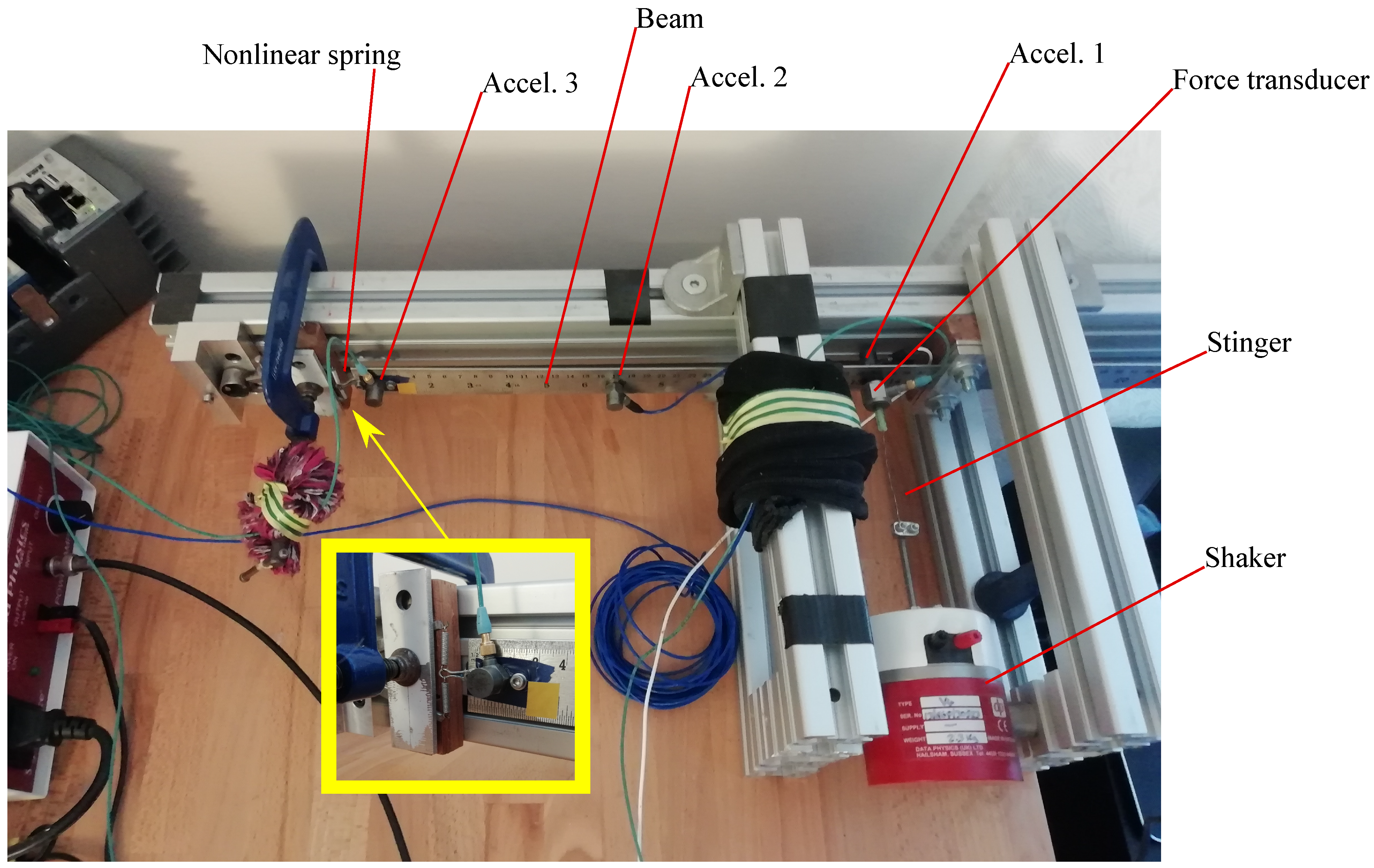
The method is applied to a nonlinear beam configuration with internally resonant coupling between modes, similar to that described in [20], and depicted in Figure 2. The stiffness nonlinearity is applied through an arrangement of tensile springs at the tip designed to reach nonlinearity through angle change, giving a response that is closely modelled by a cubic function up to displacements of approximately 7 mm. More detail on this mechanism can be found in [20]. The structure is actuated by stinger near the root as shown in Figure 2, with an accelerometer located at the same point. Therefore, integrating the acceleration signal to calculate velocity allows the calculation of PBMIF (In principle the force and velocity do not have to be obtained at exactly the same point, so long as it can be assumed that they are at $0°$ or $180°$ phase difference to one another at all frequency components of interest; indeed in [19] a voltage signal is used in a similar way with a similar assumption). Note that due to reassembly the structure cannot be assumed to have identical properties to previous publications that made use of it, but as will be seen it does show a clear 3:1 resonance between its first 2 modes.

5.2. Data Acquisition and Control

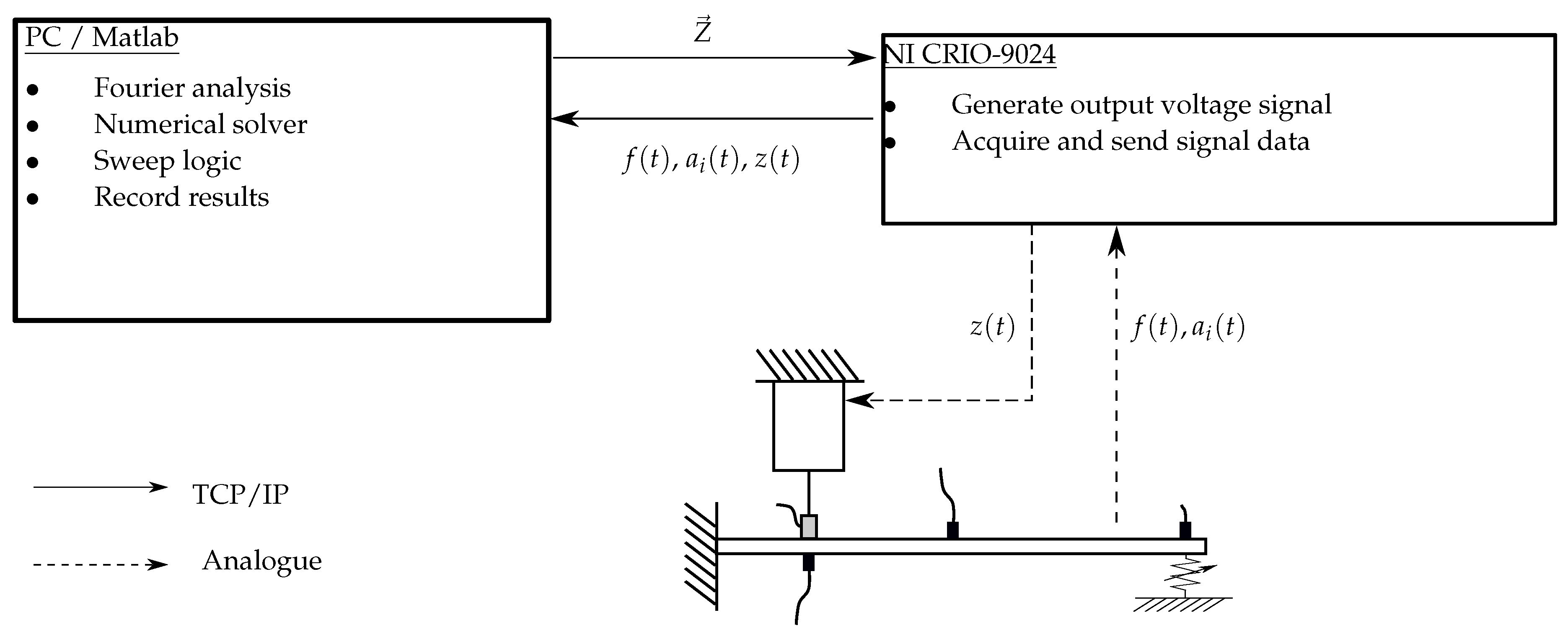
The tests are run with a National Instruments CRio-9024 Real Time controller, with a bespoke program that handles data acquisition through a NI 9234 module and outputs signals through a NI 9263 module. The sample rate is 25.6 kHz. The controller runs a bespoke program that generates voltage signals in response to a supplied vector of Fourier harmonics following the convention of Equation (4) and returns the acquired data. This is interfaced to a controlling PC via an ethernet cable using the TCP/IP network protocol. This leads to a highly flexible arrangement where, in principle, any programming language that can support TCP/IP communication (and a few low level binary operations) can be used to analyse and direct the testing process. In the present example, we have used Matlab, which additionally uses Labview’s activeX interface to automate the process of launching and terminating the real time controller. The system is summarised in Figure 3.

Data are stored in three files for each sweep. The first of these is a binary file of all time data taken during the sweep, so there is the maximum potential flexibility for future reanalysis of the test data. Secondly, a text file logs the high level actions and status of the controller, indexed to positions in the binary file, to further facilitate this analysis. Finally, a ‘.mat’ file stores the basic summary information such as Fourier coefficients of signals resolved at each point in the sweep. This gives simple access to the data such as the nonlinear FRFs presented in this document.

5.3. Settling Algorithm

The methods described all depend heavily on the assumption that the signals are periodic in nature, so the settling algorithm is an important consideration. The algorithm must be chosen as a compromise between the speed of the test, and the rejection of false data due to transient content [11]. In the present work, settling is determined based on the force signal and the acceleration signal from the beam tip. With each period of data, the vector of Fourier coefficients is formed, and this always includes all components up to the 5th harmonic, regardless of any truncation used elsewhere. Settling is determined to occur when two successive vectors are within a 1% relative change for both signals, or 100 periods have elapsed, whichever occurs first. Note that this structure can exhibit quasiperiodic responses that never settle (see [20] for an example); the presence of these responses could in principle be inferred by the relative change between successive periods still being high (e.g., ≥10%) after 100 cycles. In practice, however, it is very unlikely that a solver process will report a success for either resonance or force control under these conditions, so these cases will not appear in the results.

6. Results

6.1. Typical Resonance Seen in a Force Control Sweep

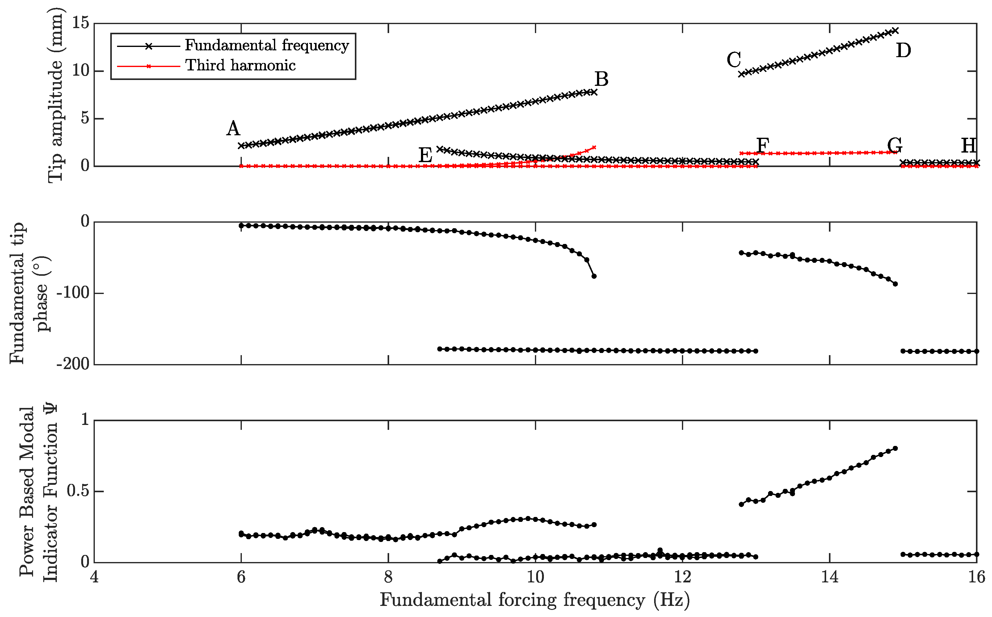
Before demonstrating a resonance controlled sweep, we examine the behaviour of the PBMIF during a force controlled sweep. Figure 4 shows combined results of a force controlled sweep rising from 6 Hz to 13 Hz in frequency, then descending again, and two sweeps initiated from the isola. The first isola sweep descends from 13.5 Hz down to 10 Hz, while the other rises from 13.5 Hz up to 16 Hz.

For a fuller explanation of features of the response of this structure, please refer to [20], however a brief summary is given here. Referring to the responses at fundamental forcing frequency in the upper graph in Figure 4, region AB is referred to as the grounded resonant region, because it can be accessed directly by stepping upwards in frequency from a low initial value. The upper termination of this region, denoted B, occurs at an approximately constant frequency and amplitude for a wide range of forcing amplitudes, because it lies above an internal resonance in the underlying backbone curve [20]. The region CD is known as an isolated resonance, or isola, and cannot be accessed by conventional frequency stepping methods. Instead, special procedures are required to activate initial conditions that settle on this branch. However, once a response is found on this branch, it is then possible to step in the usual way either upwards or downwards in frequency. Upwards stepping is terminated by a so called dropdown event at D, which will occur at higher amplitudes and frequencies when forcing is increased, in manner similar to the dropdown seen for a hardening single degree of freedom oscillator. Downward stepping will lead to dropdown at C; this is sometimes due to instability in the form of a torus bifurcation leading to quasiperiodic response. The remaining data, in regions EF and GH, all represent responses away from resonance, and are of little value to identify nonlinear terms because the low amplitudes mean that little stiffness nonlinearity is active. It would have been straightforward to obtain nonresonant data between F and G with some additional sweeps starting with non-resonant responses, however this has not been done because this reveals little about the nonlinearity or the underlying linear modes of the system. However, note that the small frequency region between C and F does reveal the existence of multiple stable responses.

It is clear from Figure 4 that the PBMIF is quite low for most of this test, particularly in the grounded resonance region, where the maximum PBMIF is 0.31. The PBMIF only exceeds 0.5 in the isola region, where it reaches a maximum of 0.8 before a dropdown event occurs. The fundamental phase graph might lead us to expect a much higher PBMIF value, given that the phase difference is 76$°$ and 87$°$ at points B and D, respectively. The difference can be explained by considering the third harmonic response amplitudes at these points, which are driven purely through nonlinearity because the third harmonic in the forcing has been set to zero. The absence of third harmonics in the force also means that the third response harmonic can make no contribution to the numerator in Equation (7). However, the third response harmonic will increase the denominator of the same equation, resulting in a decrease in $\Psi$. Furthermore, it should be noted that the PBMIF is determined by velocity amplitudes, and in these terms the third harmonic amplitude becomes three times greater in proportion to the fundamental amplitude, giving it a much greater effect than is immediately apparent from Figure 4. Finally, it should be noted that it is a matter of judicious choice of forcing that the isola exists in these results; it may not be stable for lower levels of forcing.

6.2. Resonance Control Tests

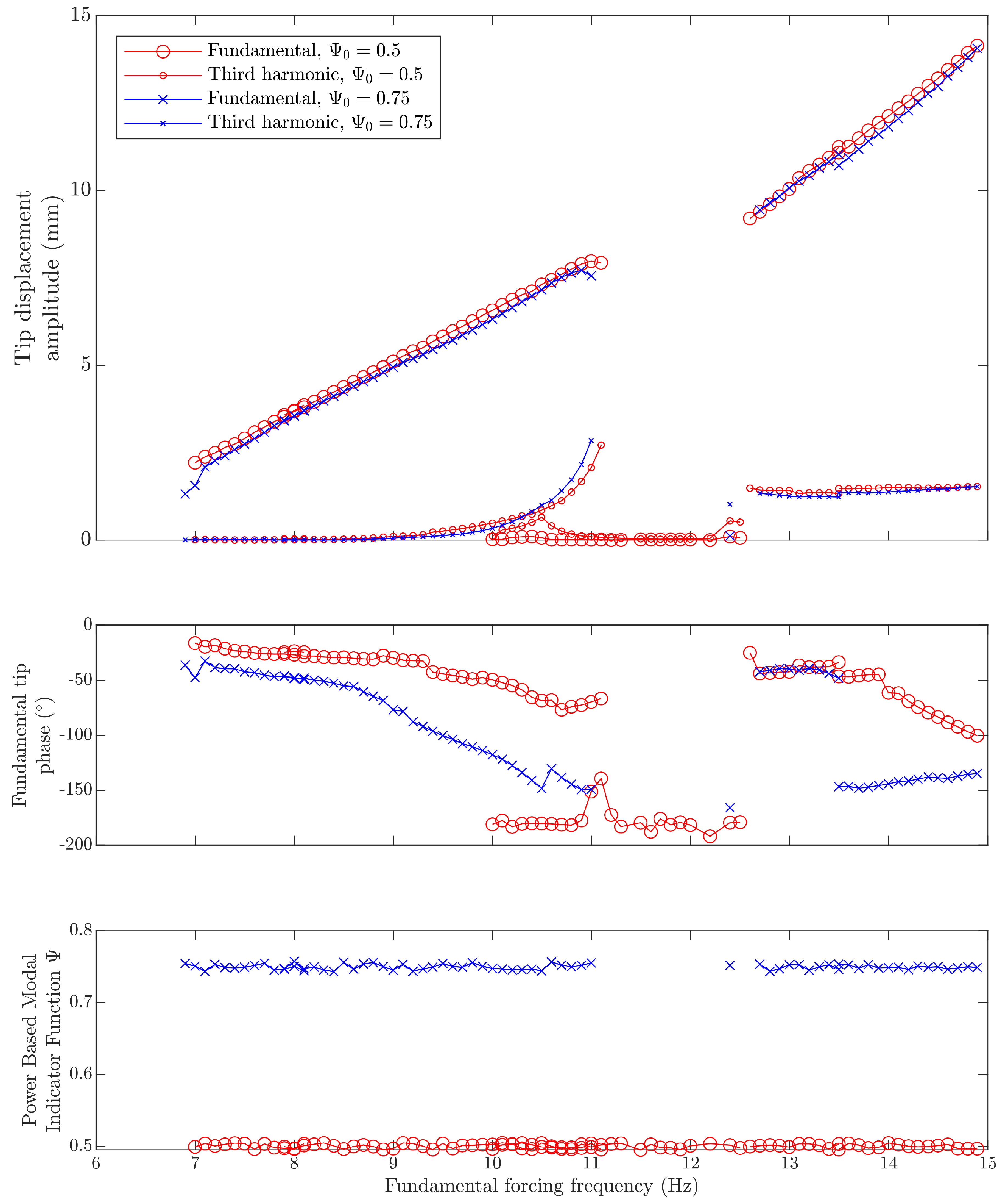
The results of resonance control are shown in Figure 5, which again shows a combination of three different sweeps for each set of results. The first sweep traces the grounded resonance region, and sweeps from 6 Hz up to 13 Hz and back down again, following the hybrid voltage/resonance control process described in Section 4.1. The two isola sweeps follow the isola initiation routine described in Section 4.2, then proceed either upwards or downward in frequency as in Section 6.1, but solving for the desired level of resonance. This was repeated for ${\Psi }_0=0.5$ and ${\Psi }_0=0.75$. Only cases where the desired level of resonance was achieved are displayed; the voltage stepping results are omitted.

An interesting phenomenon occurs during the upward sweep on the isola. Where a force control sweep on this response branch moves towards perfect resonance as frequency rises, and then drops down if it seeks to proceed further, the resonance control method will simply proceed indefinitely at constant resonance. This absence of a drop down event is a great advantage, because it means that any amplitude can be reached on this response branch. However, it does necessitate that a terminate condition is added to the logic for this sweep, to end the sweep once a certain amplitude of response is reached, to prevent destructive behaviour. Therefore the tests shown terminate when the fundamental tip amplitude reaches 14 mm.

It can also be seen that the phase graph looks somewhat noisy, particularly when we compare to Figure 4. This is because the forcing conditions for a particular degree of resonance are not generally unique, as discussed at the end of Section 2, therefore there is some scatter in the forcing and this shows up in the phase. By contrast, the forcing conditions in Figure 4 are, by definition, unique because the force is being controlled. Note that in the isola region of Figure 5, there is a large jump in the fundamental phase. This occurs at 13.5 Hz, and reflects the different forcing conditions that reach the same resonance that can be found as the solver first tries to find a solution when settling from the isola initiation procedure. The fundamental phase is also seen to range over a wide range of values on the grounded resonance branch, highlighting that angular phase is not a reliable indicator of resonance in these internally resonant systems.

Finally, a region of spurious results can be seen with very low fundamental amplitudes between 10 Hz and 12.3 Hz. These results are where the solution has dropped down from the isola branch during a downward sweep, and the solver has started finding solutions where the resonance is entirely due to the 3rd harmonic interaction with the 2nd mode of the beam, with very little fundamental amplitude.

Of course, this is not the internally resonant responses that are of interest, so a means of preventing the solver from finding these solutions would be a useful development.

6.3. Effect of Target Resonance Level

This section presents an investigation of the effect of the chosen resonance level on the responses seen. Figure 6 shows the grounded resonance region for the results of sweeps using the hybrid voltage/resonance test method of Section 4.1, for a range of ${\Psi }_0$ values. Note that a sweep was made for ${\Psi }_0=1$, but this failed to successfully solve at any frequency, and a further sweep ${\Psi }_0=0.99$ only found one solution.

It is noteworthy that varying the target PBMIF has remarkably little effect on the amplitudes of the response, either at the fundamental frequency or the third harmonic. This is also seen in the isola region of Figure 5. However, these very similar responses are being achieved under very different forcing conditions, as can be seen in the graphs of fundamental force amplitude and fundamental phase difference in Figure 6. This gives an alternative view of the amplitude saturation phenomenon noted in for example [20,27], where large changes in force amplitude give much smaller relative changes in response amplitude in the region of internal resonances. It can now be seen that lines of constant PBMIF lie very near to each other in terms of response amplitude, and hence increasing response amplitude results in a rapid loss of resonance, and therefore large increases in force amplitude are needed to give changes in response amplitude. Note that the noisy appearance of the phase and force graphs can be attributed to the non-uniqueness of the resonance controlled forcing conditions.

Finally, note that the lowest target value of ${\Psi }_0=0.5$ reaches the highest response amplitude in these tests; therefore if the objective is to obtain high amplitude data that explores the range on nonlinearity, then this is a better option. However, if the objective is to witness responses close to the underlying conservative NNM, a higher PBMIF target is preferable.

6.4. Effect of Different Levels of Harmonic Control

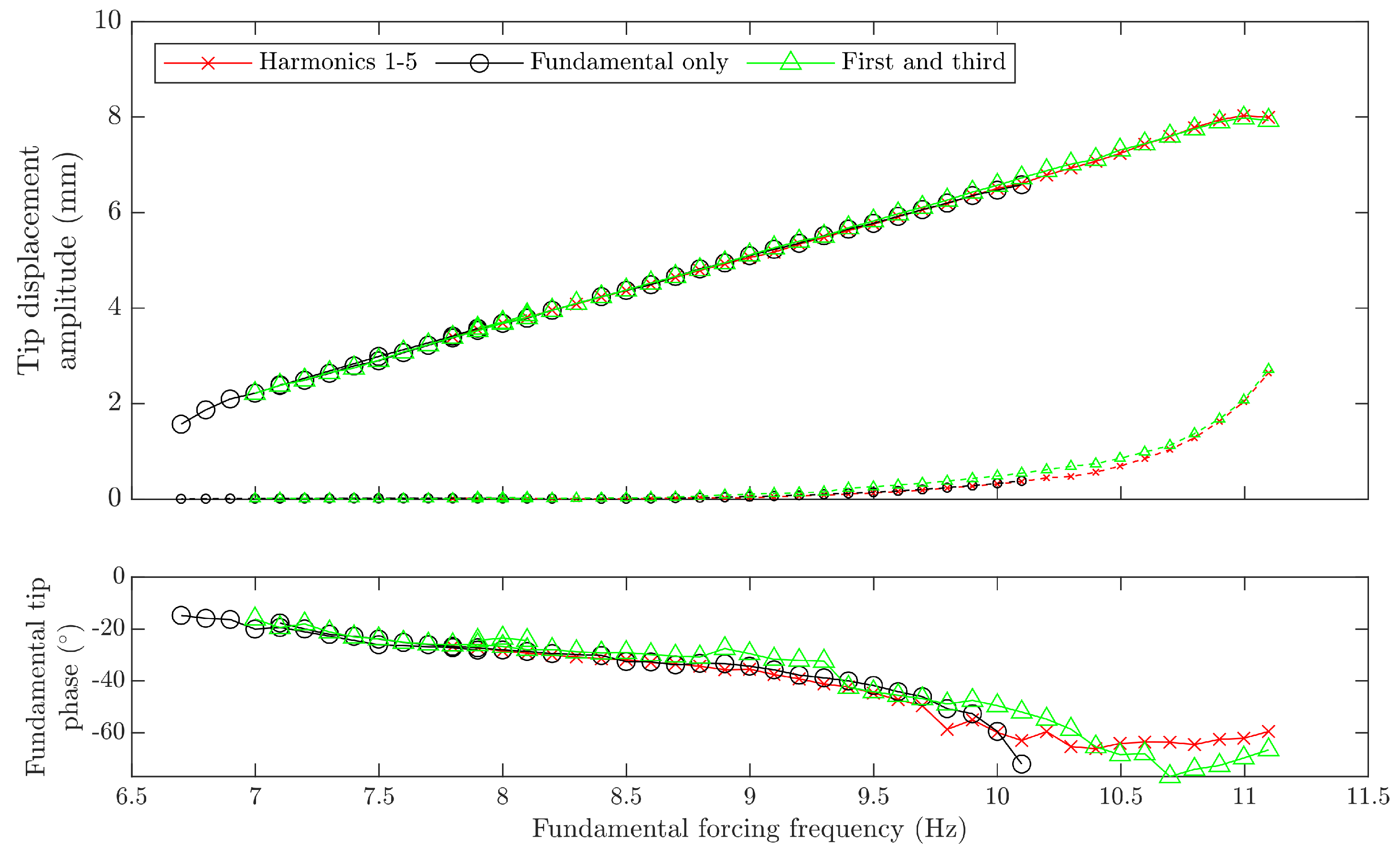
In this section, the effect of different levels of harmonic control are considered. Figure 7 and Figure 8 show the effects of varying the level of harmonic control on resonant control sweeps at ${\Psi }_0=0.5$ and ${\Psi }_0=0.75$, respectively. From these figures we can consider two features of the proposed method.

Firstly, we can compare the strategy of controlling the fundamental amplitude and third harmonic components to the more expensive approach of exciting all components up to the 5th harmonic. At the upper end of the frequency range, the two methods give results that are identical in amplitude and quite similar in terms of fundamental phase, in both figures. At the lower end of frequency range, it is seen that the ‘Harmonics 1–5’ case finds fewer valid solutions in both cases, perhaps due to the greater complexity of the input causing issues for the solver. This suggests that the ‘first and third’ strategy gives similar results to the more expensive method, and finds more solutions and is therefore a sensible choice for efficiency when a 3:1 resonance is being excited. A further advantage is that by exciting fewer harmonics, it is less likely to converge to spurious solutions as was seen in Figure 5. However, some initial characterisation would generally be needed to know if this approach was feasible.

Secondly, we can consider the potential of using an even cheaper function, where the input vector is truncated to just a single term controlling the fundamental amplitude. This means that force harmonics vary naturally in response to shaker interaction; in [21] it was found that this approach could be optimal in a force controlled identification, so long as the resulting harmonics were handled in the identification process. It is clear that this performs similarly to the other methods in many cases, although in Figure 8 it seems to find an alternative solution between 8.3 Hz and 9.2 Hz. However, the monoharmonic excitation fails to locate many higher amplitude solutions that are found by the other methods, so the additional speed of the test comes at some cost in terms of test coverage. Interestingly, the frequency at which solutions are no longer found seems to coincide with the fundamental phase being approximately $90°$.

6.5. Changes to the Structure under Test

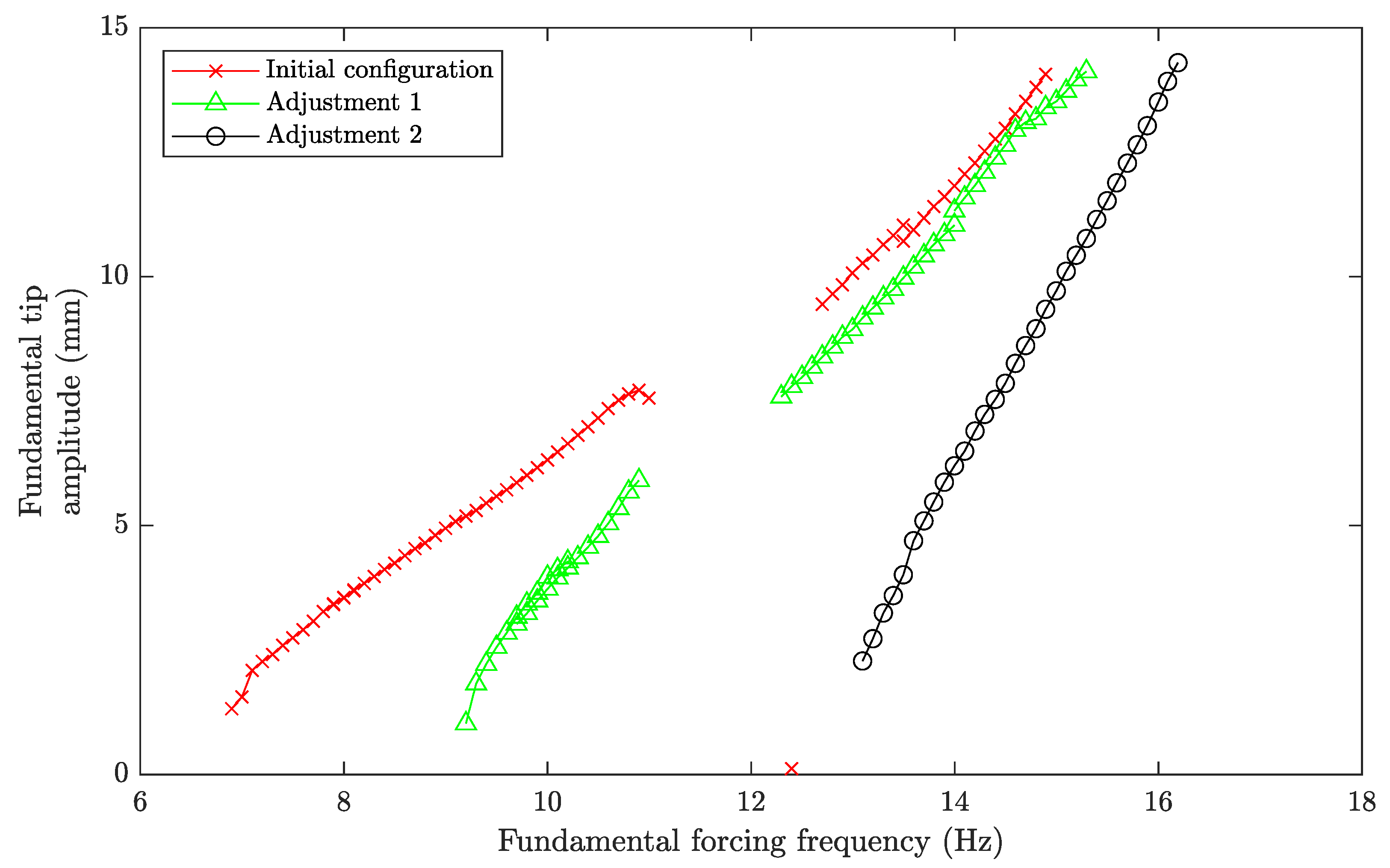
In order to consider this method on some different structural responses, the structure is altered by increasing the initial tension in the springs in the nonlinear mechanism. As can be seen in the inset to Figure 2, this can be achieved by small increases to the spacing between the upper and lower hooks that connect these springs to ground. This increases the linear stiffness applied to the tip of the beam, and thereby has a significant influence on first modal frequency. More detailed analysis of this effect can be seen in [20].

The results of this are shown in Figure 9, which compares responses at ${\Psi }_0=0.75$ for the different configurations in terms of their tip amplitudes at the fundamental frequency. The first increase in spring tension, labelled ‘Adjustment 1’ in the figure, gave results that were qualitatively similar to the initial configuration. These could be found in the same procedure as used for the initial configuration, i.e., an up and down sweep to reach the grounded resonance hump, then a downwards sweep initiated on the isolated region, and an upwards sweep initiated on the isolated region and terminated when amplitude became excessive. The only difference needed was to slightly alter the procedure needed to initiate an isola response; it was found that jumping to a starting frequency of 14 Hz initiated this solution branch more reliably than 13.5 Hz in the previous case. All other features of the algorithm remained identical to the initial configuration. It can be seen that this leads to a similar shape of response, but with the beginning of resonant responses occurring at significantly higher frequencies, and lower response amplitudes being found at each frequency. However the upper frequency of the grounded resonant region is relative unchanged; this is due to this bifurcation being strongly influenced by the 2nd linear natural frequency of the structure, which is not significantly affected by the change in stiffness at the tip.

A further increase to the spring tension is labelled ‘Adjustment 2’ in Figure 9. In this case the response is qualitatively different to the initial configuration, in that there is no isolated region of response. This meant that the resonant response could be explored in just one upward sweep that first found a resonant response at 13.1 Hz, and then proceeded upwards in frequency until excessive amplitude was encountered at 16.0 Hz. A further sweep was initiated from rest at 20 Hz and proceeded downward in frequency to 10 Hz, but in this case no new resonant responses were found. Apart from changing the frequency range of the sweeps involved, the resonant control algorithm again remained unchanged from the initial configuration.

7. Conclusions and Future Work

This work has demonstrated a passive multiharmonic testing process for internally resonant responses of nonlinear structures, that automatically seeks a desired degree of resonance, as part of a programmatically controlled sweep. It has shown how this can lead to high amplitude, resonant and feature-rich data more efficiently than traditional force controlled or monoharmonic stepped sine approaches.

It was also seen that the ideal degree of resonance to target was not necessarily the highest possible, if the aim was to reach high amplitudes, although if a near NNM response is required then higher is clearly better. It was also seen that, if the form of combination is known, only varying the specific harmonics in the excitation that correspond to this resonance gave similar results to control all of the first five harmonics. However, choosing to just excite at just a single frequency locates fewer responses, although the test can run more rapidly, and there is less chance of spurious solutions.

The highly programmable nature of the hardware setup being used opens up many possibilities that may be exploited, and this work has only just begun to explore these. Future work will consider the use of more sophisticated means of exploring the resonant response space, such as path following, rather than the current process which is currently based on constant size frequency steps.

A further area to consider is the best way for the sweep to detect resonance and switch to a resonance control algorithm. Firstly, it was found that the method of waiting for a certain resonance threshold under voltage excitation was quite a noisy indicator, and the resonant solutions would begin at quite different frequencies on different sweeps, so more robust indicators should be sought. Secondly, the work has proceeded with the advantage of the authors’ prior knowledge of the 3 to 1 internal resonance—the ideal resonance indicator would reveal this (or any other combination) automatically. This information would be useful both for identifying reduced order modelling approaches and for identifying the optimal truncation of the excitation vector. The richness of data already used in the process, including the Jacobian of the response properties, should give scope to achieve this.

Despite the improvement over conventional stepped sine testing, this process is still very slow and inefficient. So while one objective is to make it faster, an alternative strategy is to extract more value from the data that is collected. The richness of data collected, including time based transient data gathered during settling, should be exploited further, and perhaps used to produce detailed predictions for when bifurcations occur.

Finally, the authors could certainly be accused of ‘marking their own homework’ at this stage, considering that the method is applied to a well known structure specifically designed to produce many of the behaviours seen. As methods develop, they will need to be validated against a much wider variety of testbeds and real industrial structures.

References

- Wagg, D.J.; Neild, S.A. Nonlinear Vibration with Control; Springer: Dordrecht, The Netherlands, 2009. [Google Scholar]
- Ewins, D.J. Modal Testing: Theory, Practice, and Application; Mechanical Engineering Research Studies: Engineering Dynamics Series; Research Studies Press: Baldock, UK, 2000. [Google Scholar]
- Ewins, D.J.; Weekes, B.; Delli Carri, A. Modal testing for model validation of structures with discrete nonlinearities. Philos. Trans. R. Soc. A 2015, 373, 20140410. [Google Scholar] [CrossRef]
- Kerschen, G.; Worden, K.; Vakakis, A.F.; Golinval, J.C. Past, present and future of nonlinear system identification in structural dynamics. Mech. Syst. Signal Process. 2006, 20, 505–592. [Google Scholar] [CrossRef] [Green Version]
- Wang, X.; Khodaparast, H.H.; Shaw, A.D.; Friswell, M.I.; Zheng, G. Localisation of local nonlinearities in structural dynamics using spatially incomplete measured data. Mech. Syst. Signal Process. 2018, 99, 364–383. [Google Scholar] [CrossRef] [Green Version]
- Noël, J.P.; Kerschen, G. Frequency-domain subspace identification for nonlinear mechanical systems. Mech. Syst. Signal Process. 2013, 40, 701–717. [Google Scholar] [CrossRef]
- Peeters, M.; Kerschen, G.; Golinval, J.C. Modal testing of nonlinear vibrating structures based on nonlinear normal modes: Experimental demonstration. Mech. Syst. Signal Process. 2011, 25, 1227–1247. [Google Scholar] [CrossRef] [Green Version]
- Peeters, M.; Kerschen, G.; Golinval, J.C. Dynamic testing of nonlinear vibrating structures using nonlinear normal modes. J. Sound Vib. 2011, 330, 486–509. [Google Scholar] [CrossRef] [Green Version]
- Scheel, M.; Peter, S.; Leine, R.I.; Krack, M. A phase resonance approach for modal testing of structures with nonlinear dissipation. J. Sound Vib. 2018, 435, 56–73. [Google Scholar] [CrossRef]
- Londoño, J.M.; Neild, S.A.; Cooper, J.E. Identification of backbone curves of nonlinear systems from resonance decay responses. J. Sound Vib. 2015, 348, 224–238. [Google Scholar] [CrossRef] [Green Version]
- Friswell, M.I.; Penny, J.E.T. Stepped sine testing using recursive estimation. Mech. Syst. Signal Process. 1993, 7, 477–491. [Google Scholar] [CrossRef]
- Sieber, J.; Gonzalez-Buelga, A.; Neild, S.; Wagg, D.; Krauskopf, B. Experimental continuation of periodic orbits through a fold. Phys. Rev. Lett. 2008, 100, 244101. [Google Scholar] [CrossRef] [Green Version]
- Barton, D.A.W.; Mann, B.P.; Burrow, S.G. Control-based continuation for investigating nonlinear experiments. J. Vib. Control 2012, 18, 509–520. [Google Scholar] [CrossRef]
- Renson, L.; Gonzalez-Buelga, A.; Barton, D.; Neild, S. Robust identification of backbone curves using control-based continuation. J. Sound Vib. 2016, 367, 145–158. [Google Scholar] [CrossRef] [Green Version]
- Renson, L.; Shaw, A.; Barton, D.; Neild, S. Application of control-based continuation to a nonlinear structure with harmonically coupled modes. Mech. Syst. Signal Process. 2019, 120, 449–464. [Google Scholar] [CrossRef] [Green Version]
- Renson, L.; Sieber, J.; Barton, D.; Shaw, A.; Neild, S. Numerical continuation in nonlinear experiments using local Gaussian process regression. Nonlinear Dyn. 2019, 98, 2811–2826. [Google Scholar] [CrossRef] [Green Version]
- Peter, S.; Leine, R.I. Excitation power quantities in phase resonance testing of nonlinear systems with phase-locked-loop excitation. Mech. Syst. Signal Process. 2017, 96, 139–158. [Google Scholar] [CrossRef]
- Karaağaçlı, T.; Özgüven, H.N. Experimental modal analysis of nonlinear systems by using response-controlled stepped-sine testing. Mech. Syst. Signal Process. 2021, 146, 107023. [Google Scholar] [CrossRef]
- Ehrhardt, D.A.; Allen, M.S. Measurement of nonlinear normal modes using multi-harmonic stepped force appropriation and free decay. Mech. Syst. Signal Process. 2016, 76–77, 612–633. [Google Scholar] [CrossRef]
- Shaw, A.; Hill, T.; Neild, S.; Friswell, M. Periodic responses of a structure with 3: 1 internal resonance. Mech. Syst. Signal Process. 2016, 81, 19–34. [Google Scholar] [CrossRef] [Green Version]
- Shaw, A.D.; Hill, T.L.; Neild, S.A.; Friswell, M.I. Experimental Identification of a Structure with Internal Resonance. In Nonlinear Dynamics; Springer: Berlin/Heidelberg, Germany, 2016; Volume 1, pp. 37–45. [Google Scholar]
- Virgin, L.N. Introduction to Experimental Nonlinear Dynamics; Cambridge University Press: Cambridge, UK, 2000. [Google Scholar]
- Detroux, T.; Noël, J.P.; Virgin, L.N.; Kerschen, G. Experimental study of isolas in nonlinear systems featuring modal interactions. PLoS ONE 2018, 13, e0194452. [Google Scholar] [CrossRef] [Green Version]
- Gatti, G.; Brennan, M.J. Inner detached frequency response curves: An experimental study. J. Sound Vib. 2017, 396, 246–254. [Google Scholar] [CrossRef] [Green Version]
- Yasuda, K.; Kawamura, S.; Watanabe, K. Identification of nonlinear multi-degree-of-freedom systems. Presentation of an identification technique. JSME Int. J. Ser. 3 1988, 31, 8–14. [Google Scholar] [CrossRef] [Green Version]
- Hill, T.; Neild, S.; Cammarano, A. An analytical approach for detecting isolated periodic solution branches in weakly nonlinear structures. J. Sound Vib. 2016, 379, 150–165. [Google Scholar] [CrossRef] [Green Version]
- Czaplewski, D.A.; Chen, C.; Lopez, D.; Shoshani, O.; Eriksson, A.M.; Strachan, S.; Shaw, S.W. Bifurcation generated mechanical frequency comb. Phys. Rev. lett. 2018, 121, 244302. [Google Scholar] [CrossRef] [PubMed] [Green Version]
Figure 1.
Flow chart for testing process.
Figure 2.
Photo of test rig, with inset detailing the nonlinear spring mechanism.
Figure 3.
Diagram of controller.
Figure 4.
Results of a force control sweep, fundamental force amplitude 2.75 N, third harmonic force amplitude set to zero through feed forward control; other harmonics not controlled.
Figure 5.
Resonance controlled frequency sweeps, with voltage excitation applied at the fundamental frequency and third harmonic (small markers indicate third harmonic values).
Figure 6.
Resonance controlled frequency sweeps, with voltage excitation applied at the fundamental and third harmonic frequencies (small markers indicate third harmonic values).
Figure 7.
Resonance controlled frequency sweeps with different levels of harmonic control, (Small markers indicate third harmonic values).
Figure 8.
Resonance controlled frequency sweeps, with different levels of harmonic control, (Small markers indicate third harmonic values).
Figure 9.
Effect of variation of the spring tension in the nonlinear mechanism on resonance control sweeps, .
© 2020 by the authors. Licensee MDPI, Basel, Switzerland. This article is an open access article distributed under the terms and conditions of the Creative Commons Attribution (CC BY) license (http://creativecommons.org/licenses/by/4.0/).
Share and Cite
MDPI and ACS Style
Shaw, A.D.; Hill, T.L.; Neild, S.A.; Friswell, M.I. Multiharmonic Resonance Control Testing of an Internally Resonant Structure. Vibration 2020, 3, 217-234. https://0-doi-org.brum.beds.ac.uk/10.3390/vibration3030017
AMA Style
Shaw AD, Hill TL, Neild SA, Friswell MI. Multiharmonic Resonance Control Testing of an Internally Resonant Structure. Vibration. 2020; 3(3):217-234. https://0-doi-org.brum.beds.ac.uk/10.3390/vibration3030017
Chicago/Turabian StyleShaw, Alexander D., Thomas L. Hill, Simon A. Neild, and Michael I. Friswell. 2020. "Multiharmonic Resonance Control Testing of an Internally Resonant Structure" Vibration 3, no. 3: 217-234. https://0-doi-org.brum.beds.ac.uk/10.3390/vibration3030017