
Axisymmetric Hybrid Plasma Model for Hall Effect Thrusters
by
 ,
,
Mario Panelli
1,* ,
,
Davide Morfei
2, 
Beniamino Milo
3,
Francesco Antonio D’Aniello
4 and
Francesco Battista
1,*
1
CIRA, The Italian Aerospace Research Centre, Via Maiorise, 81043 Capua, Italy
2
University of Rome “La Sapienza”, 00184 Rome, Italy
3
University of Naples “Federico II”, 80138 Naples, Italy
4
University of Campania, “Luigi Vanvitelli”, 81100 Caserta, Italy
*
Authors to whom correspondence should be addressed.
Particles 2021, 4(2), 296-324; https://0-doi-org.brum.beds.ac.uk/10.3390/particles4020026
Submission received: 30 April 2021
/
Revised: 11 June 2021
/
Accepted: 12 June 2021
/
Published: 18 June 2021
Abstract
:Hall Effect Thrusters (HETs) are nowadays widely used for satellite applications because of their efficiency and robustness compared to other electric propulsion devices. Computational modelling of plasma in HETs is interesting for several reasons: it can be used to predict thrusters’ operative life; moreover, it provides a better understanding of the physical behaviour of this device and can be used to optimize the next generation of thrusters. In this work, the discharge within the accelerating channel and near-plume of HETs has been modelled by means of an axisymmetric hybrid approach: a set of fluid equations for electrons has been solved to get electron temperatures, plasma potential and the discharge current, whereas a Particle-In-Cell (PIC) sub-model has been developed to capture the behaviour of neutrals and ions. A two-region electron mobility model has been incorporated. It includes electron–neutral/ion collisions and uses empirical constants, that vary as a continuous function of axial coordinates, to take into account electron–wall collisions and Bohm diffusion/SEE effects. An SPT-100 thruster has been selected for the verification of the model because of the availability of reliable numerical and experimental data. The results of the presented simulations show that the code is able to describe plasma discharge reproducing, with consistency, the physics within the accelerating channel of HETs. A small discrepancy in the experimental magnitude of ions’ expansion, due probably to boundary condition effects, has been found.
1. Introduction
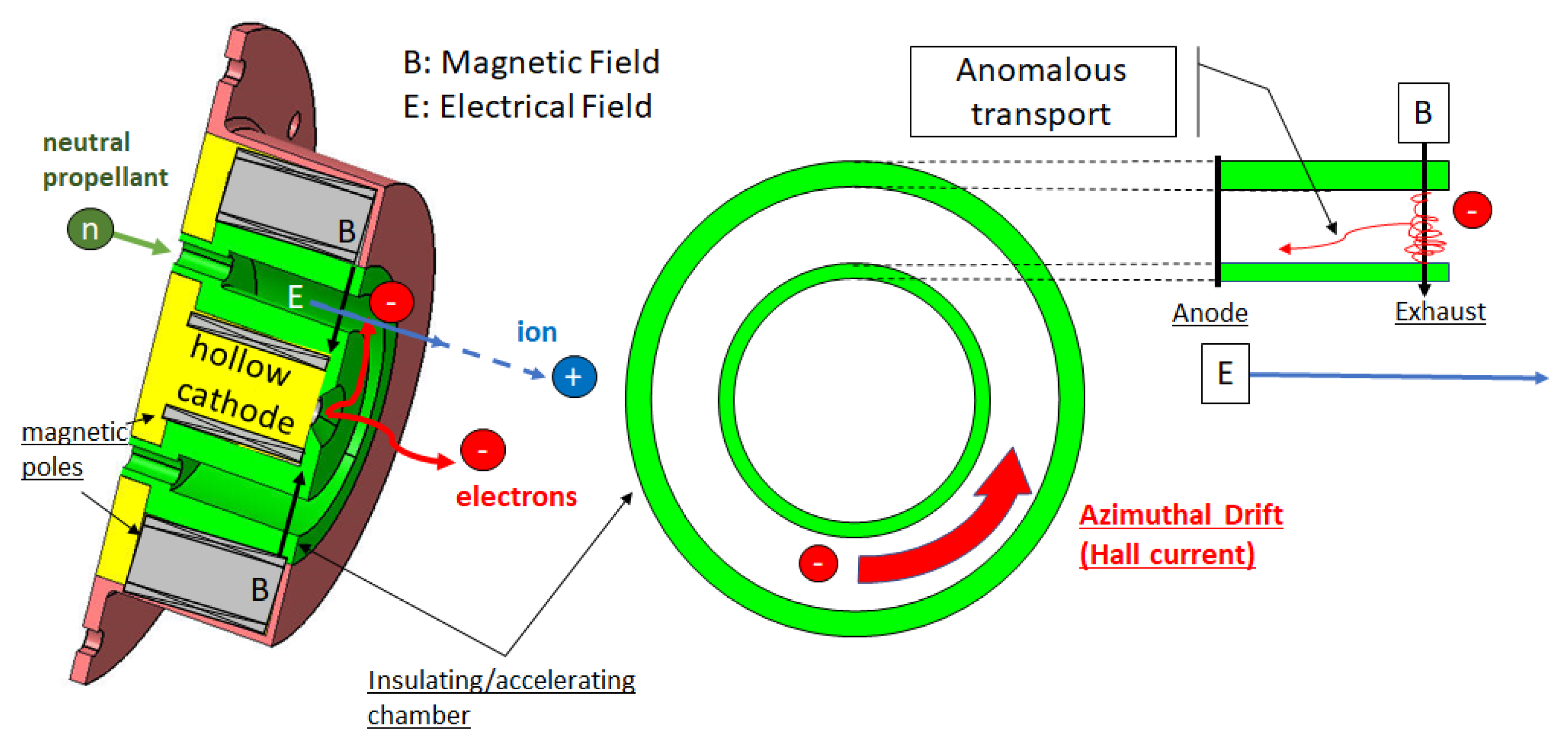
Hall Thrusters are spacecraft propulsion devices that utilize applied magnetic fields and closed electron Hall drift to accelerate quasi-neutral plasma [1]. The typical Hall Thruster consists of an annular chamber with one end open to the ambient environment (Figure 1). A neutral propellant is injected through the closed end, which also contains the anode. An externally located cathode produces electrons, a fraction of which enters the chamber and ionizes the propellant, and the other part neutralizes the ions in the plume. In order to increase the electron transit time, and hence improve the ionization efficiency, magnetic field (B) is applied over a section of the chamber. The magnetic field strength is selected such that electrons become magnetized and trapped in a closed azimuthal Hall drift at about the thruster centreline. The magnetic field thus plays an important secondary role. Since the field restricts motion of electrons in the normal direction, electrons redistribute along the magnetic field line according to the spatial variation in ion density. The magnetic field lines thus become lines of constant potential and an electric field (E), which develops in the direction normal to the magnetic field, accelerates the ionized propellant. The direction of acceleration thus depends on the topology of the magnetic field. In most of the HETs configurations, the magnetic lines are not perfectly perpendicular to the chamber. Thus, a beam divergence occurs that pushes ions also toward the channel. Ions with enough energy collide with the wall and remove part of material due to sputtering. The channel wall material (typically a ceramic) protects the magnetic circuit from hazardous particles. Once the magnetic circuitry is exposed to plasma, the thruster’s end of life is declared.
Despite over 40 years of flight heritage, the community still requires tools capable of modelling these devices to predict their lifetime and because, in spite of important research efforts, there is still the lack of understanding of such phenomenology that limits their full potential development, e.g., electrons transport across the magnetic field [2]. For the last purpose, various numerical models have been developed. Time-accurate solvers are used because HETs are subjected to various types of instabilities and oscillations, e.g., the ionization instability (called “breathing mode”), which is due to the periodic depletion and replenishment of neutral atoms in the ionization region and leads to current oscillations in the 10–20 kHz frequency range [2].
Simulations address either the near or far regions of the plasma plume, since the regimes in which they operate are quite different from the point of view of the “main” physical effects in the plasma. Typical approaches for the channel and near-plume regions are: kinetic, fluid and hybrid modelling.
In kinetic models (cf., e.g., [3,4,5,6,7,8]), electrons and heavy species (ions and neutrals) are treated as discrete particles and their trajectory is followed in the space phase considering the action of electric and magnetic fields. Monte Carlo Collisions (MCC) algorithms are often used to manage collision between particles. The majority of particle codes are based on the Particle-In-Cell (PIC) methodology, in which macro-particles, representatives of a number of real particles, are first sorted and “weighted” to a spatial mesh, which is utilized to calculate the electric and magnetic fields. This method provides the velocity distribution function (VDF) of species, but computational cost is very high because of the small time step required to follow electrons.
In fluid modelling (cf., e.g., [9,10,11]), all species involved in the plasma discharge are modelled as fluids. The fluid equations use the framework of the Boltzmann equation to describe the evolution of macroscopic quantities of interest. Each equation depends on moments, whose evolution is given by equations of higher order; therefore, the equations need to be truncated, or “closed”, at a certain order. In order to do this, an assumption can be made on the shape of the VDF (e.g., Maxwell distributions), which is used to derive a closed expression for the moment of the highest order to be conserved in the equations. This approach is computationally efficient, but the main limitation is due to the inability to solve for “kinetic” effects, which are those associated with how the various processes in the discharge affect the shape of VDF.
A compromise between previous models is represented by hybrid modelling (cf., e.g., [12,13,14,15,16,17,18,19]), typically choosing a kinetic approach for the heavy species populations, and the fluid approach for the electron population. Among the kinetic approaches, PIC is preferred to other combinations (such as Direct Kinetic, solving kinetic equations [20]) because it allows for describing accurately the VDF of heavy species, reducing computational efforts. The main limitation of hybrid-PIC simulations is the necessity of anomalous coefficient’s fluid electron description. It has been known since the early studies of HETs that collisions between electrons and neutral atoms (defined as the “classic” contribution mechanism to electrons’ mobility) are not sufficient to explain electron transport across the magnetic field lines, especially in the exhaust region where the magnetic field is maximum and the atom density is very small due to intense ionization inside the channel [21]. Various theories [1,16,17,22,23] have been proposed to explain this anomalous electron transport (e.g., electron–wall scattering, field fluctuations, Bohm diffusion) but a self-consistent model, able to accurately predict the operation of HETs and to help in designing new thrusters, is yet to be determined. Despite this limitation, hybrid models have been one of the preferred approaches over the past two decades in the simulation of HETs’ acceleration channel and plume, being able to model some of the high-level physical interactions that are responsible for the behaviour of these devices.
The HYbrid PIC-FLUid model (HYPICFLU) described in this paper is based on the legacy and lessons learned mainly from the HYbrid PIC-Hall (HPHall) code by Fife [13], and its development, Hybrid PIC Hall-2 (HPHall2) [16,17,24], but it takes also ideas from Hageelar et al. [18] and Kawashima et al. [15].
HPHall is one the first hybrid codes to model HETs that is able to reproduce “breathing mode” oscillations. It uses a PIC approach on an axisymmetric domain (2D radial-axial) and quasi-one-dimensional fluid equations for electrons, with magnetic field lines as spatial coordinates (thermalized electrons assumption, cf. [25]). The domain includes the channel and part of the near-plume region that is shaped with a circular sector. In order to accommodate the domain, a non-uniform spatial grid is used for the PIC method. A mixed electron mobility model (“classic”+“anomalous”) with one empirical parameter accounting for Bohm diffusion is used. In order to consider the effect of the Secondary Electron Emission (SEE) on the mobility, a total near the wall-current is modelled and included in the current conservation equation. Ions are generated as the result of electron–neutral collisions. Despite that only single-charge ions are tracked by PIC, an ionization rate for double-charge ions, a function of the single-charge ions density, can be enabled. Finally, HPHall uses an energy independent cross section for electron–neutral (Xenon) scattering of 30 × 10 m.
HPHall-2, the evolution of HPHall, includes the following main changes: the modification of the algorithms for injection, reflection, and recombination of neutrals at the walls; the inclusion of ion-neutral collisions and plasma–wall interaction (i.e., the fulfilment by the ion flow of the Bohm condition required by the sheath solution, the inclusion of the “wall-collisionality” phenomenon, the adoption of new sheath model [24] which distinguishes between primary and secondary electrons and takes into account the space-charge saturation for high SEE). HPHall-2 uses a two region mixed mobility model for the electrons: the value of the empirical parameter for Bohm diffusion differs from inside to outside of the channel and a linear variation allows for a smooth transition at the exit of channel. Furthermore, electron–ions and electron–wall collision frequencies are included in the contribution of the mobility. The first one is modelled using the classic formula with the Coulomb logarithm [26] whereas the second one is derived by the new sheath model implemented, which is a function of axial coordinates and several plasma properties [17]. Finally, an energy dependent function of electron–neutral frequency, based on the Maxwellian average of the measured Xenon cross section of Nickel et al. [27], is considered.
HYPICFLU inherits from HPHall/HPHall-2 the hybrid approach using PIC on an axisymmetric domain (2D radial-axial) and 1D approximation to the electron fluid, but, to simplify the implementation process and several functions (e.g., the “sorting” and “weighting” function), a uniform Cartesian mesh on rectangular domain shape, including the channel and near-plume region, has been selected. The electron flux on the upper and lower boundaries outside the channel is set to be zero according to Kawashima et al. [28]. With the purpose to study in a first extent low-discharge voltage thruster (less than 300 V), the effects of multiple charged ion species on the plasma response have been neglected, as common practice in the literature [16,17,18,19]. The mobility model is similar to that used by HPHall-2 in which it differs by: the calculation of electron–neutral collision frequency which uses a new correlation for the most recent elastic electron–neutral cross section for Xenon [29]; the calculation of the electron–wall collision frequency by means of the simpler model proposed by Hageelar et al. [18], which considers wall collision to be constant within the channel throughout an empirical parameter (in range) that multiplies the typical measured frequency of s; a continuous function that allows for the transition of Bohm empirical parameters from the value set within the channel to that outside. The location and the width of the axial position interval in which the variation occurs are considered as free parameters. Moreover, because near-wall current is not calculated, the effect of SEE on the mobility is incorporated into the internal Bohm coefficient.
Finally, the sheath model is similar to HPHall [12] and the algorithms for injections, ionization and wall recombination are inherited from HPHall-2 [17].
The aim of this paper was to describe and document the principles of the model implemented in HYPICFLU and the simulation results of SPT-100 discharge are presented in order to verify the simulation potential of the models implemented with respect to relevant experimental data and numerical models from the literature.
2. Hybrid PIC-Fluid Approach for HET Plasma
The unknown plasma variables of the HYPICFLU model are:
- , ion number density;
- , neutral particle density;
- , ionization rate;
- , ion velocity vector;
- , neutral velocity vector;
- , electron temperature;
- , plasma potential.
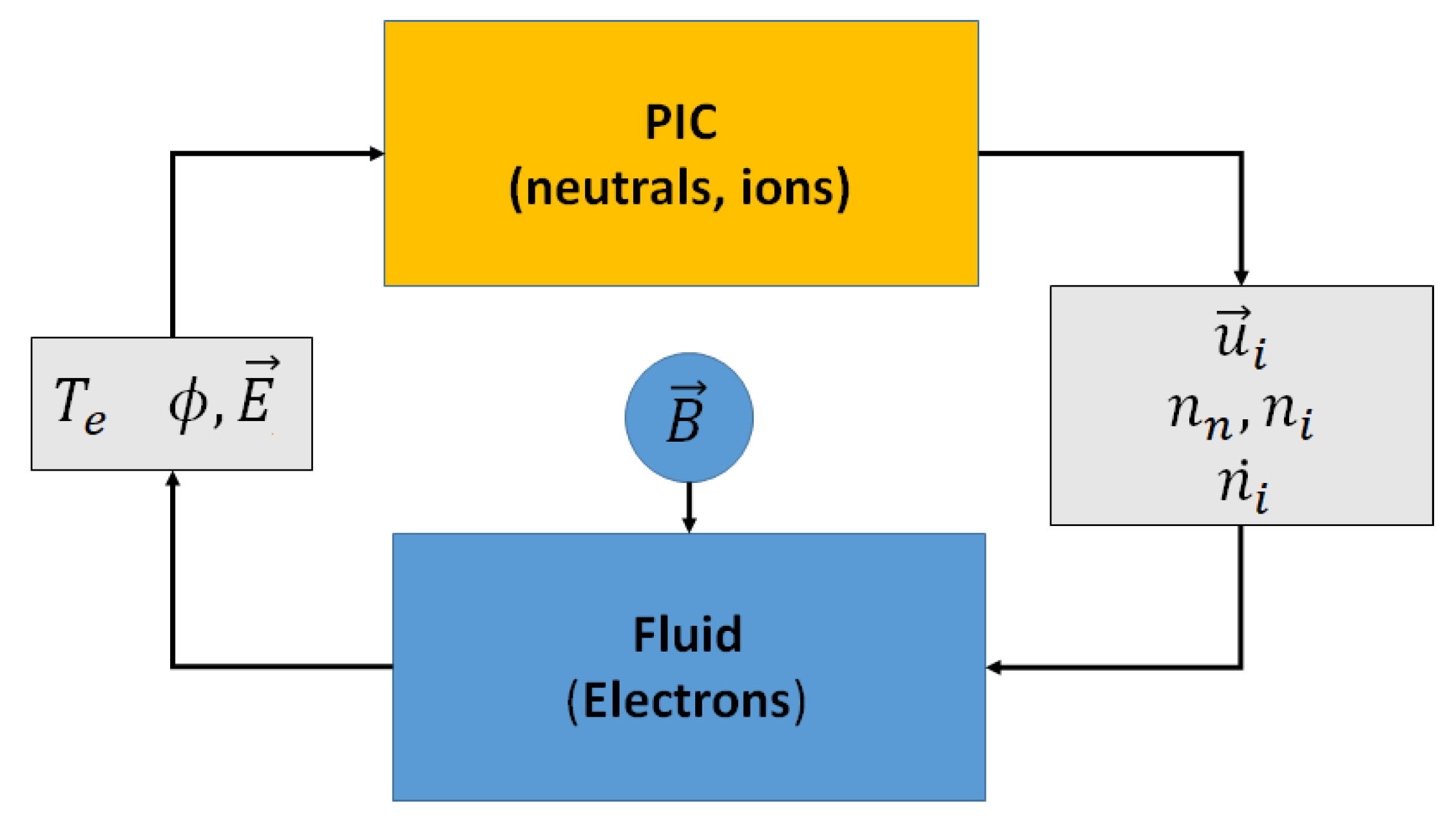
The model is composed of two parts: the Particle-In-Cell (PIC) sub-model, for the heavy species (i.e., ions and neutral), and the fluid one, for electrons. Figure 2 shows the data exchanged between them. All variables are time dependent, except for magnetic field, . This means that the sub-models interact iteratively since the outputs of one are used as inputs of the other and vice-versa.
Particularly, fluid electrons equations require as input the number density of both ions and neutrals (), the velocity of ions () and the ionization rate () and return the electron temperature () and the plasma potential (), from which we derive the electric field () that accelerates ions in the channel; on the contrary, the heavy species sub-model needs as inputs electron temperatures and electric fields and gives back both the number density of ions and neutrals, the velocity of ions and the ionization rate. Neutrals velocity () is computed by PIC but it is not required by the fluid sub-model.
Bulk plasma is quasi neutral (i.e., ) and a proper sheath model for plasma interaction with walls are taken into account in the fluid equations.
The magnetic field is an external input of only the fluid sub-model because only electrons are magnetized.
2.1. Heavy Particles
Heavy particles, i.e., ions and neutrals, are modelled with the PIC method. Each simulated particle represents an agglomerate of real particles, typically to , saving computational time (a code simulating each particle would be resource intensive, indeed). The number of particles represented by one computational macro-particle is called specific weight and, in general, it varies among the particles and changes with time, e.g., due to ionization. The mass of one macro-particle is obtained by multiplying the mass of the single particle with the specific weight.
One limit of the PIC method is the introduction of numerical oscillation (“noise”) due to its inability to simulate a continuum of particles. The specific weight plays a major role in this sense: the lower it is, the less the numerical fluctuations are because more particles are simulated.
The governing equations for the PIC method are the laws of dynamics. Particularly, the second one, written for a generic charge particle subjected to both electric () and magnetic fields (), is:
where is the acceleration, is the charge to mass ratio of the macro-particle and is its velocity.
The second term on the RHS of Equation (1) can be neglected since both neutrals and ions are not magnetized (i.e., their motion is slightly influenced by the magnetic field because their Larmour radius is larger than the typical channel length). Hence, the acceleration is:
For neutrals, having no charge, it reduces to . Equation (2) can be integrated each time-step in order to update particles’ velocity and position.
Neutrals are injected from the inlet that is modelled as an annular ring positioned at the centre of anode wall. Velocities of new-injected particles are sampled from a semi-Maxwellian distribution characterized by anode wall temperature [30].
Neutral–neutral and ion–neutral collision are neglected within the channel because typically neutrals mean the free path is higher than the channel length. Hence, a macro-neutral changes its velocity only if a wall collision occurs. Following Ref. [16], neutrals that undergo a collision with the walls are scattered back in the domain diffusively with a velocity sampled from a Maxwellian distribution at the wall temperature. Usually, the gas–surface interaction is modelled with the Maxwell scattering model, in which a fraction of the colliding particles are reflected diffusively while the remaining are reflected specularly, where is the accommodation factor. However, the complete accommodation, that is the purely diffusive reflection, describes well the interaction of the neutrals with the walls of a Hall Thruster [31]. In fact, the sputtering and the reposition tends to increase the roughness of the walls inside HETs, which is the primary cause of the random distribution of the reflected particles [16].
It is assumed that every ion colliding with the wall recombines into a neutral, with a velocity that, again, is sampled from a semi-Maxwellian distribution at the wall temperature.
Only the ionization due to neutral–electron collisions is modelled and only single ionized ions are considered. Double ionized ions can produce appreciable effect on the performances, especially for thrusters operating at high power levels; however, a precise characterization of the discharge is beyond the aims of this work. The ionization rate, i.e., the rate at which ions are created per unit of volume, can be expressed as [13]:
Here, is the ionization rate, is the ionization coefficient while and are respectively the electron and neutral number densities (for quasi-neutrality ). is a function only of the electron temperature (e.g., approximate formula for Xenon can be found in [1]). The bulk recombination has not been modelled because it is several orders of magnitude inferior to the bulk ionization rate, as shown in [13].
Finally, it is worth underlining that, by neglecting the neutral–ion collisions, this excludes the possibility of charge exchange (CEX), which produces slow ions and fast neutrals, everywhere. The effect of CEX is significant in the plume where it can lead to the attraction of slow ions toward the thruster. However, since CEX modelling requires the development of complex algorithms such as Monte Carlo Collision (MCC) that are computational demanding and, since the effect in the thruster performances is quite limited, the CEX has been neglected.
2.2. Electrons
The electron fluid equations used in the fluid sub-model are: the electrons momentum equation, current conservation and electron energy equations. The parameters that can be computed are the electron temperature (), the discharge current (), the plasma potential () and the electron velocity normal to magnetic streamlines (). As a result of quasi-neutrality in the bulk plasma, electron density () is known as the result of the PIC sub-model, i.e., .
2.2.1. Momentum Equation
Since the electrons inside the acceleration zone are magnetized and assuming that they reach thermal equilibrium, the electron momentum equation, along a magnetic field line, can be written as:
where is the Boltzmann constant, e is the electron charge and denotes the tangent vector to the magnetic field lines.
Integrating Equation (4), it is possible to obtain:
where the RHS term () is known in the literature as thermalized potential [25], and it is constant along a magnetic field line. The thermalized potential assumption allows to reduce the dimension of the problem to quasi-one-dimensional (Q1D); thus, the fluid domain is mono-dimensional. This means that both the potential and electron temperature are constant along the magnetic field streamlines (), but they vary with them, i.e., .
Electron diffusion across the magnetic field is assumed to obey a generalized Ohm’s Law:
where denotes the normal vector to magnetic field lines and is the electron mobility across the magnetic field line.
By knowing the relationship between the derivatives along and the derivatives with respect to (Equation (A7)) and by utilizing the definition of thermalized potential Equation (5) and Equation (6) can be finally written as:
where B is the magnetic field intensity. Equation (7) states that the electron velocity across the magnetic streamlines depends on electron temperature and thermalized potential; hence, it is function of .
The electron mobility is modelled as a combination between the classical and anomalous contributions, accounting for plasma turbulence and collisions with neutrals, ions and walls:
Here, is the electron mass; and are the electron–ion/neutral collision frequencies; is the electron–wall collision frequency. The coefficient k is chosen empirically; generally, it ranges from 0 to 0.1 in the channel and it assumes a value equal or higher than 1 outside [16,17,18,23]. The wall collision frequency ranges between s and s, according to the model proposed by Haagelar et al. [18]. Since mobility depends on empirical parameters, the model is not self consistent.
2.2.2. Current Conservation
To conserve current:
where is the current collected by the anode while and are the electron and ion current, respectively. Near-wall current was not included and its contribution has been regarded by varying opportunely the coefficients of electron mobility mentioned above.
Equation (9) can be rewritten considering a surface obtained rotating magnetic streamline () on the thruster axis:
thus, the integrals are performed along . Here and are the ion and electron velocity normal to magnetic streamline whereas r is the radial coordinate.
Expanding the electron velocity normal to (Equation (7)) and simplifying, it is possible to obtain the derivative of thermalized potential:
2.2.3. Electron Energy Equation
The electron energy equation can be written as:
where the RHS of Equation (12) takes into account the elastic and inelastic collision terms, and represent the heat conduction.
Particularly,
where is the heat conduction coefficient found with the assumption that heat and mass diffuse in the same way.
The term is the joule heating due to elastic collision and can be expressed as:
where is the electron flux.
The inelastic collision term, represents the energy loss due to ionization and excitation of neutrals and ions. The energy loss due to the excitation of neutrals is significant and can not be neglected, while the excitation of ions is at least two orders of magnitude smaller and it is not considered. In addition, since double-ionized ions are not modelled, their contribution on is disregarded.
The excitation of neutrals can be modelled increasing the ionization energy with the energy associated with the excitation of neutrals:
Here, is the ionization energy, is the cross section of excitation from the ground state to the energy state and is the cross section of the ground state ionization. An analytic solution of Equation (15) is given by Dugan et al. [32] and it can be fitted [13] as:
where A, B and C are coefficients related to the gas considered while and z are respectively the normalized ion production cost and electron temperature:
2.2.4. Boundary Conditions
Equation (11) is integrated to compute thermalized potential assuming Dirichlet Boundary Conditions (BC) at both cathode and anode line, .
Equation (12) is integrated to get electron temperature assuming Neumann BC at the anode, (indeed the relatively small magnitude of the magnetic field at the anode allows to assume an infinitely large diffusion across a magnetic field line) and a Dirichlet BC at the cathode line,
The electron energy loss to the wall is:
Here, is the electron flux in the bulk of the plasma, i.e., where the plasma is not affected by the sheath; is the temperature of the secondary electrons emitted (∼1 eV); is the wall potential, calculated as:
where and are respectively the Bohm and the most probable thermal velocity of electron, whereas the Secondary Electron Emission (SEE) yield (), that is the ratio between the emitted secondary electrons and the incident primary electrons, can be written using the Euler’s Gamma Function ():
Here, A and B are two constants that depend on the wall material (e.g., A = 0.123 and B = 0.528 for BoroSil [17]).
When the electron temperature is lower than a certain limit, the break-up temperature (i.e., ), the wall potential is negative. This mean that only the most energetic electron passes the sheath, arriving at the wall; thus, the electron flux to the wall is limited in this condition. Equation (20a) is used. When , the sheath collapses, the wall potential reaches values near and this filtering action disappears; thus, the wall losses increase dramatically. Equation (20b) is used.
3. Numerical Model
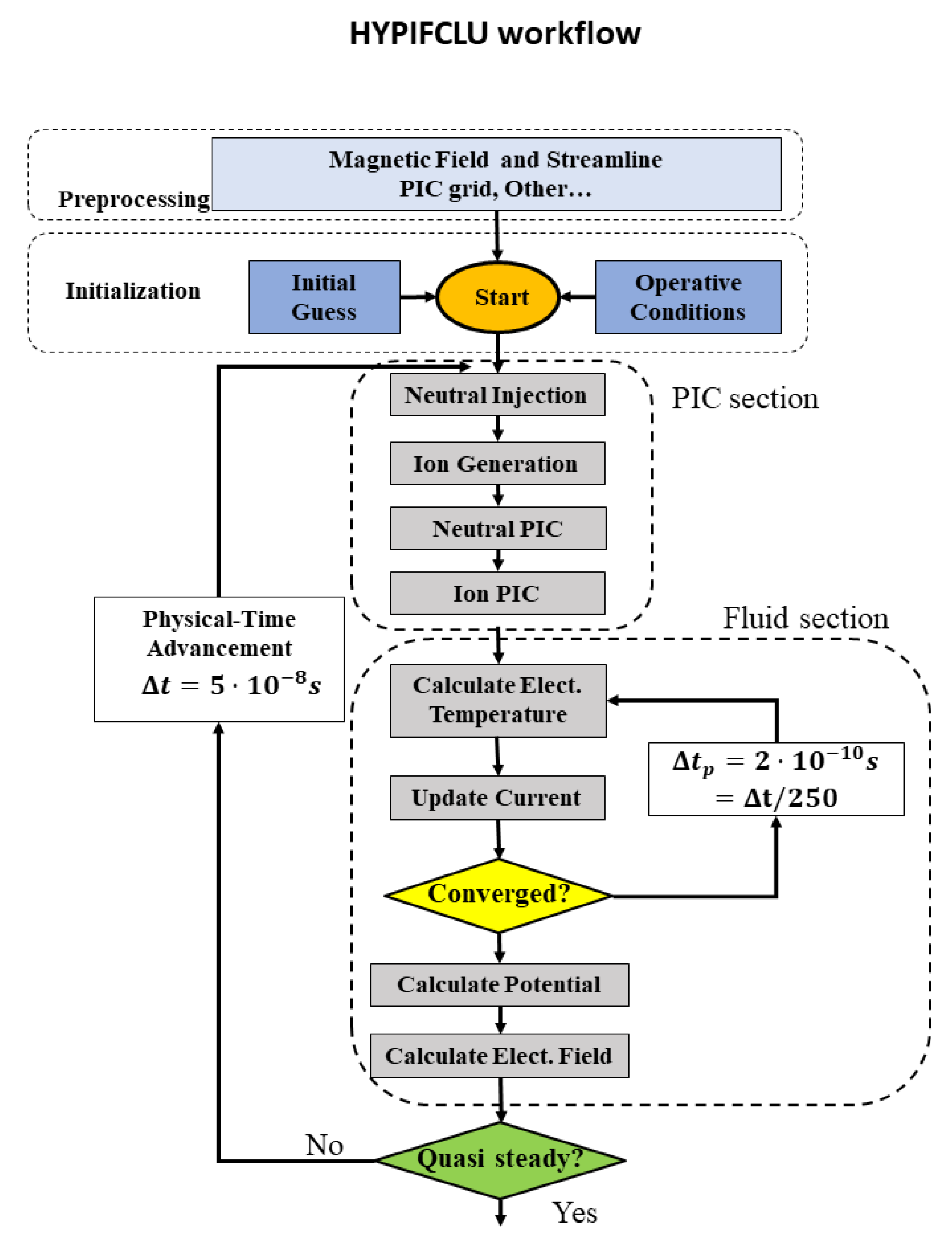
Figure 3 shows the flow chart of the HYPICFLU code. The pre-processing phase includes the generation of both domain and mesh for PIC sub-model and the definition of the magnetic streamlines (Appendix A). After the initialization computation starts. In a typical iteration of the code, at first the equations of heavy particles’ motion are integrated, then the fluid equations are solved while the quantities related to the heavy particles, i.e., neutral and ion density, their velocities and the ionization rate, are kept constant. The governing equations of the heavy species (neutrals and ions) and electrons are integrated over the same time interval but different timescales: typically (cf. [12,13,19,24]), the time step of the fluid equations ( s) is two orders of magnitude smaller than the PIC one ( s).
3.1. Particle-In-Cell for Heavy Particles
The computational domain for the PIC method in the HYPICFLU code is a rectangle that, starting from the anode, includes the channel of the thruster and part of the near plume region.
The area is fully meshed using a uniform Cartesian grid because of the simplicity it offers in its construction, as well as for the sorting and weighting methods and for the computation of gradient fields, which may be required throughout the simulation. Additionally, it can help in avoiding undesired non-physical effects, which may appear in highly deformed meshes related to the calculation of volumetric forces over the macro-particles [5]. Cell size has been selected as a compromise between accuracy and computing efforts. Indeed, by reducing its dimension, the spatial accuracy of the resulting field is improved but more macro-particles are required to reduce numerical noise.
Each heavy particle is characterized by its position, velocity, specific weight, mass and charge. To update position and velocity, the equations of motion (Section 2.1) are integrated using Leap-frog scheme. The time step, , is such that the distance travelled by a particle must not be greater than the typical length of a cell [24]; thus, the maximum value that can be used is simply calculated subdividing the dimension of cell by the theoretical exhaust velocity (i.e., the maximum value expected in the domain). This guarantees the satisfaction of Courant stability criterion for the Leap-frog Algorithm, because [33].
Particles are not pushed in cylindrical coordinates but in a 3D Cartesian system; after the push, they were rotating back to the r–z plane (for details see [34]). Electric field, required to push ions (Equation (2)) is calculated by a fluid sub-model, interpolated to the grid nodes and successively gathered [35] to particle position.
The ionization process is divided into two different steps: first, an integer number of macro-ions are created in each cell according to the ionization rate defined over the nodes and then mass is removed from each macro neutral in order to ensure the mass conservation [13,24]. Ionization rate (Equation (3)) is computed using the electron temperature provided by fluid sub-model and interpolated to the nodes.
At the end of each time-step, particle velocity and mass are scattered [35] to the grid nodes. This information, along with ionization rate, is used as the input to solve fluid equations.
The recombination of ions on the walls is based on a Monte Carlo algorithm. Neutrals and ions are characterized by two different specific weights; particularly, being that neutral density is higher than ions density, neutral specific weight is higher (about 2 orders of magnitude). When an ion macro-particle impacts the wall, a random number in the range 0–1 is generated and compared to the ratio between ion and neutral specific weights. If this number is less than the ratio (i.e., about 0.01), the ion macro-particle is removed and a neutral is injected. To verify the algorithm, a series of ions with a fixed position and velocity were fired on a wall. In particular, the mass of neutrals created was compared with mass of ions destroyed. The results have shown that the error was below 5.
3.2. Fluid Electrons Equations
Equations (9) and (12) form a determined system with unknowns and that are solved iteratively until a number of pseudo time steps () to equal one PIC time step () has been completed (Figure 3). Then, thermalized potential () is obtained integrating Equation (11); using the definition of thermalized potential (Equation (5)), it is possible to compute the plasma potential () and consequently, by deriving, the electric field ().
It is possible to verify that Equation (11) can be rewritten as a function of the derivative of electron temperature to :
where and are functions of such quantities provided by the PIC sub-model and the discharge current (see Appendix B for details). Knowing the electron temperature distribution, it is easy to integrate Equation (23) to get the thermalized potential. Equation (23) can also be manipulated and used to calculate the discharge current, if electron temperature and thermalized potential fields are provided.
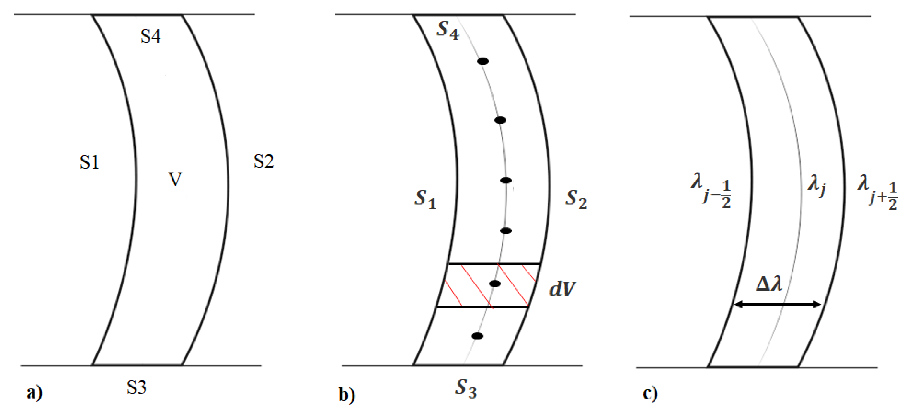
Equation (12) is solved by means of a Finite Volume Method (FVM) taking into account that electron temperature can vary only with the magnetic streamlines (Q1D problem) as consequences of the thermalized potential assumption. Thus, Equation (12) is integrated using a volume element delimited by two consecutive magnetic streamlines () and the up/down boundary of the domain (), Figure 4a, within which electron temperature can be assumed to be constant.
The discretized form of the equation is:
where k is the time iteration, is the time interval and:
Here, j is the index of the fluid element, which corresponds to the jth magnetic streamline (MS), Figure 4c. The “fluid mesh” is thus defined by the magnetic streamlines, the number of which states the grid refinement level, and the surfaces and correspond to and (Figure 4c). The distance () between two consecutive MSs is set to be constant. By considering for convenience at the anode boundary, the developed algorithm searches in the domain for iso- lines spaced by ; as requirements, every MS must go with continuity from the lower to upper boundaries of the domain. The lines identified with this method are and (defined as “lateral”) and the jth magnetic streamline (“central”) lays in the middle. It is worth noting that, with this approach, the number of MSs is not known a-priori but it depends strictly on .
The factors in Equation (24) are a function of the quantities provided by the PIC sub-model and the discharge current (see Appendix B for details). They are obtained by integrating along magnetic field lines, which are divided into a number of discrete points for this purpose. The volume integrals of the ith fluid element are calculated over the ith streamline (Figure 4b), while the surface integrals over and are calculated over the streamlines and . On all these nodes the data calculated by the solution of fluid equations are available. Thus, an interpolation to PIC mesh is due in order to be used for the next step. It is worth noting that the number of points along a magnetic streamline is selected to be close to that of the PIC mesh along the radial coordinate and the number of magnetic streamlines is about the number of axial nodes of the PIC mesh, in order to reduce interpolation errors.
The last two terms in Equation (24) refer to, respectively, the inelastic losses (Equation (19)) and the wall losses (). The wall losses, modelled using Equation (20), are true only if the surfaces are within the channel. Outside, according to Kawashima et al. [28], it was neglected ().
Thus, using a Forward Time Centred Space method (FTCS) for the time derivatives and solving the “space” derivatives by using a central scheme, the electron temperature at the pseudo-time step k + 1 can be computed.
It can be verified that Equation (24) can be rewritten as a linearized Burger’s equation with some additional terms [13]. Thus, the convective-diffusive criterion for the stability criterium for FCTS can not be applied directly, but it can be used for an iterative search of stable pseudo time steps. Thus, several runs for identical conditions were executed with different pseudo time steps: the selected value corresponded to the case where the solution was stable (i.e., electron temperature, discharge current and potential as function of pseudo time step converge to a stable value) and it does not vary considerably with inferior time step [13].
3.3. Code Development and Validation
Extensive efforts were undertaken to verify the results of the model. All new segments of the code were tested and compared with hand calculations before the next segment was begun. In this way, the techniques of ”top-down design” and ”step-wise refinement“ were used to make sure bugs were kept to a minimum. For this purpose, every function was tested stand-alone before being included in the model. For each case, experimental or numerical data were selected to compare the results. Disparities between computed and reference data were carefully examined as possibly due to bugs in the code. Particularly, several verification tests of PIC and fluid module stand-alone were conducted but they are not reported here for the sake of brevity.
4. Results
In this section, the code is used to rebuild suitable experimental data and to perform also comparison with some relevant numerical models presented in the literature. Particularly, the simulation of SPT-100 thruster discharge is selected as a crucial validation test case because a lot of experimental and numerical data about the plasma inside and outside the accelerating channel of the thruster are available (cf., e.g., [16,17,19,28,36]).
The following subsections will give the reader details about SPT-100 and they will provide a concise and precise description of the model results, compared to experimental and numerical data, and their interpretation, as well as the conclusions that can be drawn.
4.1. SPT-100 Thruster
The SPT-100 is a Hall-effect thruster designed and built in Russia by the Experimental Design Bureau Fakel which has over 15 years of on-orbit flight heritage on a Russian spacecraft with this thruster. SPT-100 is a 1.35 kW thruster and it has been well developed and proven for satellite applications. A variety of derivatives based on the SPT-100 [37] have been also built and flown. One of them has flown for the Earth–Moon Mission [37], too.
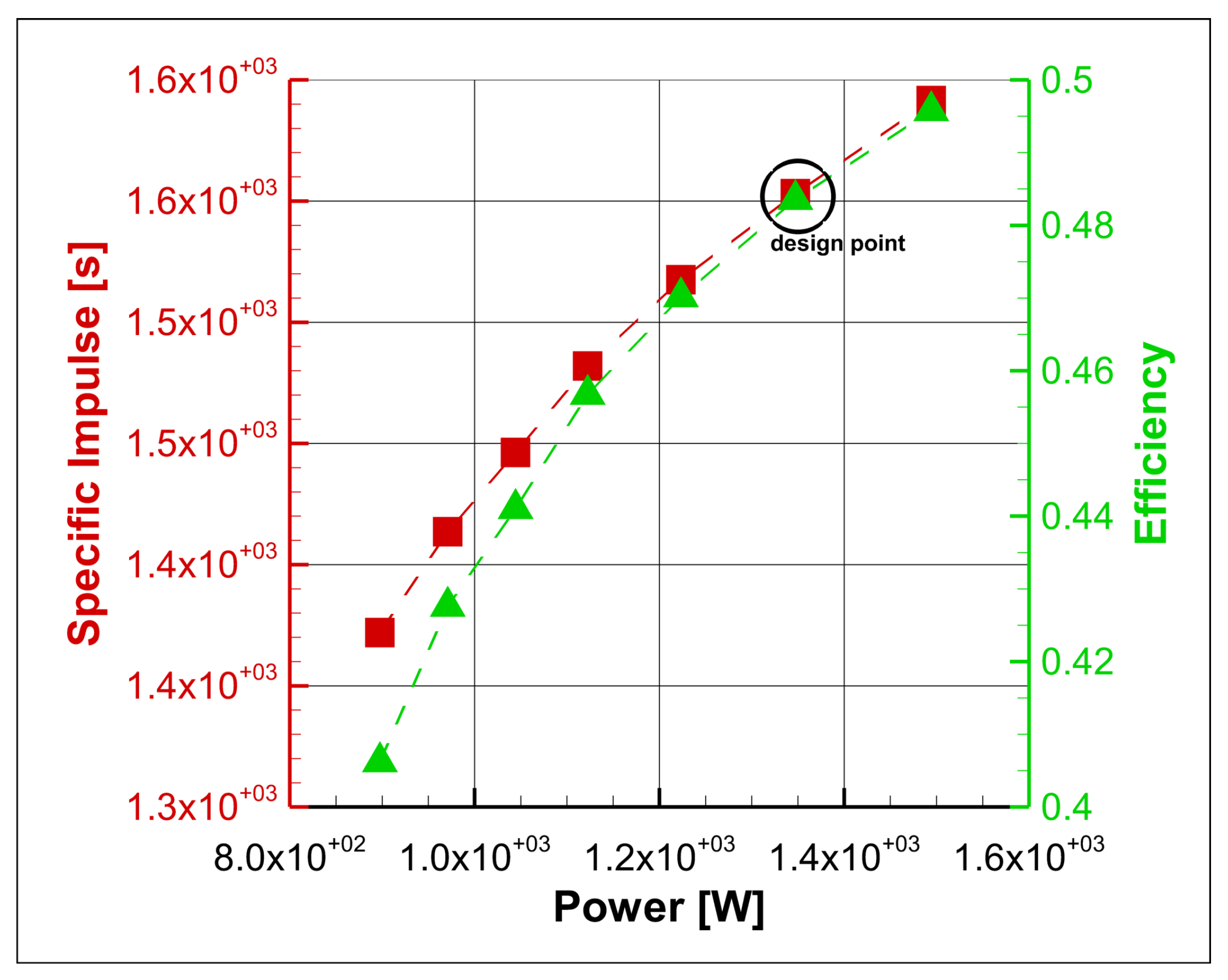
Figure 5 shows a picture of SPT-100 where it is visible the external magnetic coils which generate the magnetic field. Figure 6 shows the performance of SPT-100. For the present study, the design point condition has been selected (black circle in Figure 6). Finally, Table 1 reports its dimensions and nominal operative conditions [38].
4.2. SPT-100 Discharge Simulation
This section reports the results of two tests (Table 2) performed to assess that the code is able to reproduce SPT-100 discharge. The results are compared to the available numerical and experimental data.
The tests mainly differ by the grid refinement level: uniform Cartesian grids with square cells and 25 × 7 (coarse grid) and 49 × 13 (fine grid) nodes are respectively used. Cell dimensions are respectively 0.25 and 0.125 mm. Fluid grid resolutions have been selected to be as close as possible to the PIC grid, in order to reduce interpolation errors. The spacings between the magnetic streamlines are respectively Vm and Vm.
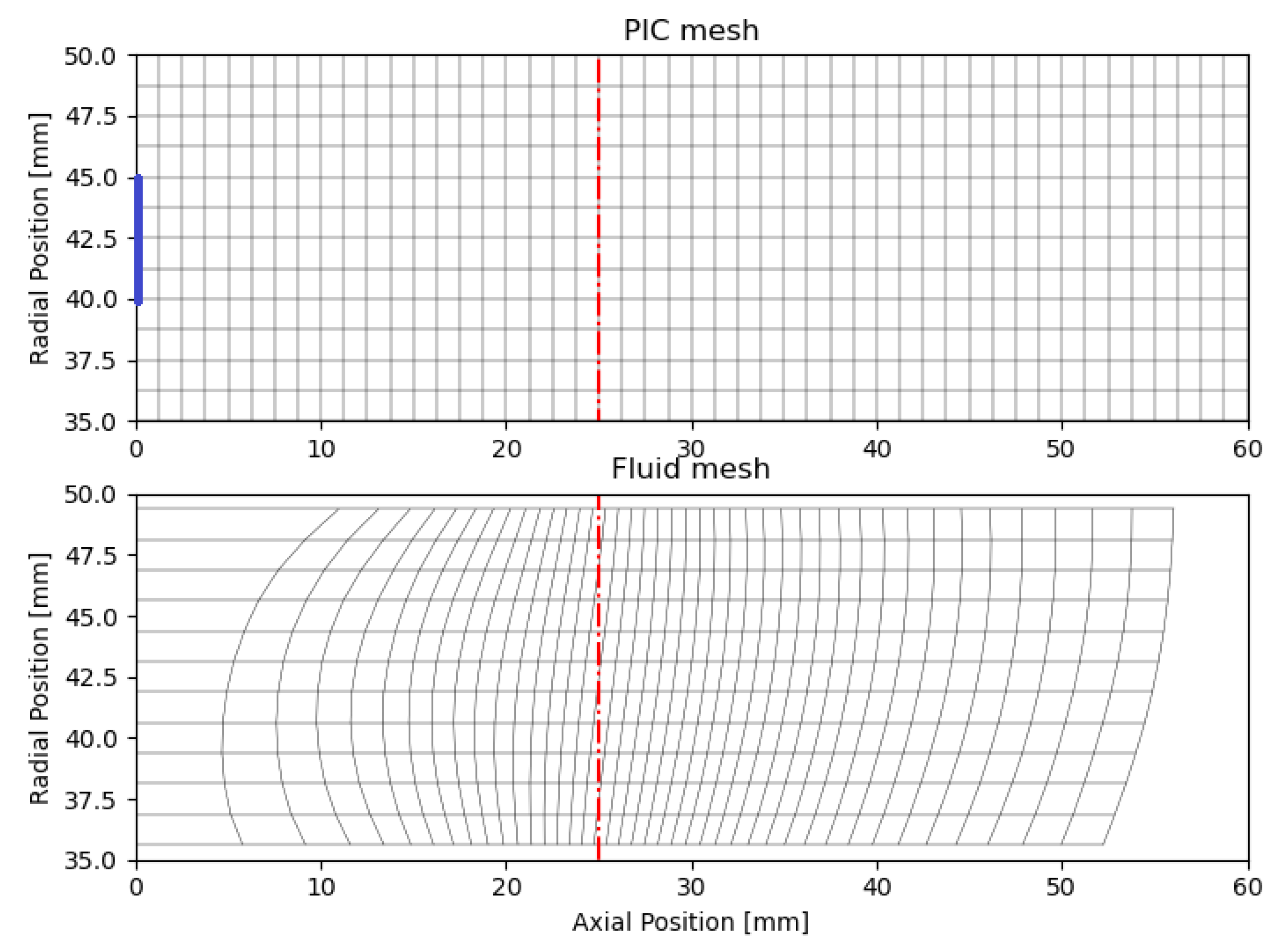
Figure 7 shows as an example the two meshes used in Test 106 calculation. Neutral particles are injected into the domain throughout the cells between radial positions 40 and 45 mm (blue line in Figure 7). Fluid grid nodes are the points used to discretize the “lateral” magnetic streamlines (cf. Section 3.2). Particularly. the last raw of nodes are used to represent the cathode.
PIC time step and the pseudo-time step, used to integrate the electron energy equation, are respectively s and s, for both calculations. The first one guarantees that one macro-ion advances no more than one cell per time step (stability requirement, cf. Section 3.1) in both tests and it is calculated subdividing cell’s dimension by the theoretical exhaust velocity of SPT-100 (∼20 km/s), calculated as [1], where is the ion mass (i.e., Xenon). The pseudo-time step is selected to ascertain that the fluid solver converged (cf. Section 3.2) and the solution does not vary considerably with inferior values.
A trade-off analysis was needed to get the specific weights (Table 2) that allowed to smooth numerical “noise” due to the limitations of the PIC method in simulating a continuum of heavy particles. It was found, in accordance with the literature [19,24], that specific weights allowing to get an average number of macro-particles per cell higher than 30 fulfilled this task.
Bohm/SEE contributions to mobility outside and inside the channel have been empirically set. As a first guess, the values reported by Hofer et al. [17], 0.035 and 1, have been used, but a sensitivity analysis, using coarse grid, has shown that, to fit the plume trends, a higher value is needed (i.e., 5). To assess grid effect, these values are retained also in Test 106 using a finer grid. Inside the channel, the mobility model includes an electron–wall collision frequency of s. The electron–neutral collision frequency is evaluated using the cross section formula proposed in Ref. [29].
It is important to review the boundary conditions. Neutrals are reflected on channel walls with a diffuse-reflection scheme and ions impinging on the wall are neutralized and neutrals diffuse according to the same scheme; the anode and channel walls are respectively set to 750 K and 850 K according to Ref. [17]; the cathode, as seen above, is a magnetic streamline that represents the external boundary of the fluid domain. A Dirichlet BC on electron temperature is set at the cathode (4 eV). A linear variation of is assumed downstream of the cathode where the electron temperature at the boundary of the PIC domain is kept fixed at 0.1 eV [13]. Cathode’s potential is set to 10 V and 0 V is applied at the end of domain. A potential drop of 300 V is established between the anode and cathode. A current of about 4.5 A is expected.
4.2.1. Magnetic Field Calculation
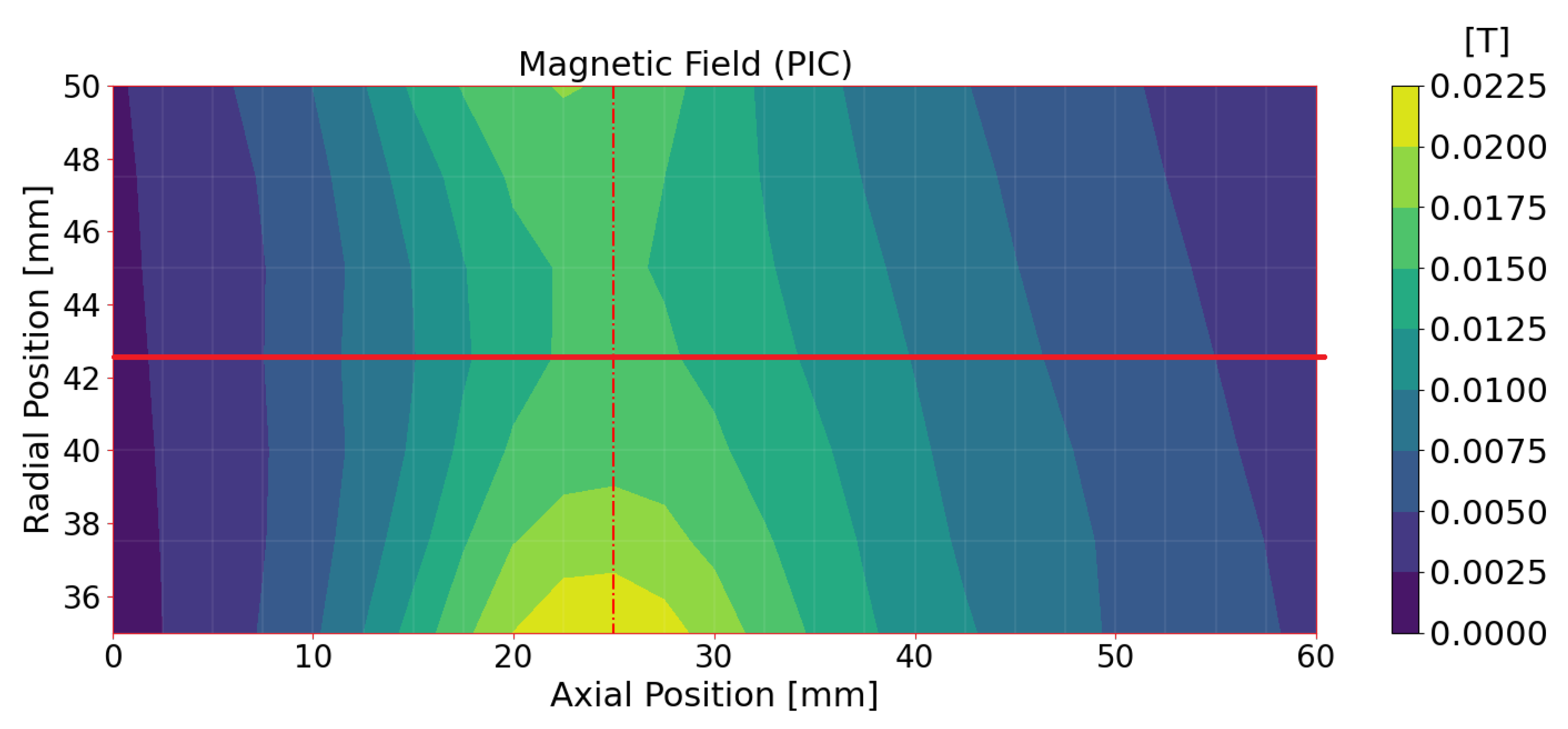
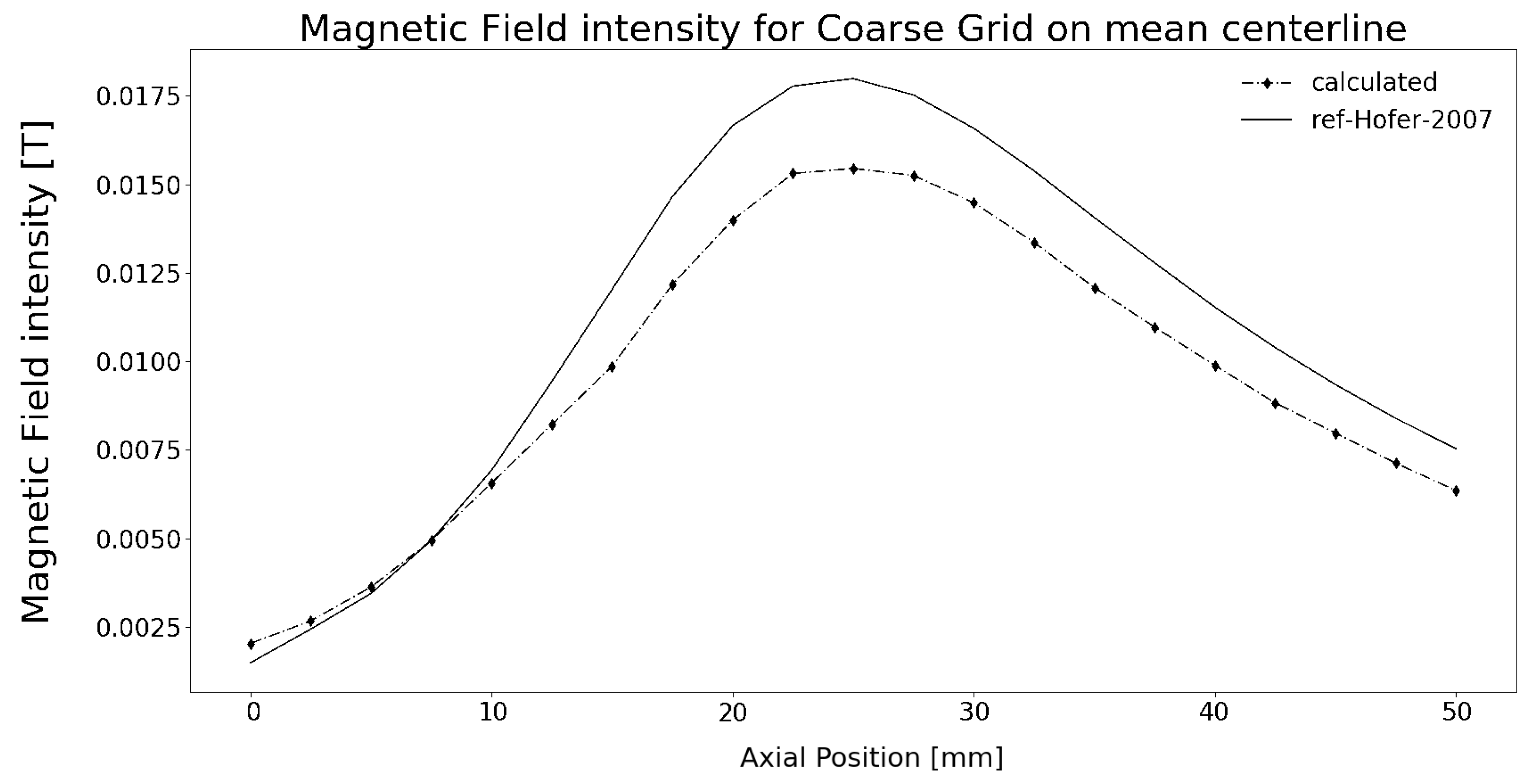
SPT-100 magnetic circuit behaviour was reproduced using FEMM software [41]. It has been adjusted until the trend of radial magnetic field along the channel centreline (radial position = 42.5 mm) assumed a Gaussian axial profile in accordance with the literature [17,28] and the value at the exit section was close to that reported in Table 1. Figure 8 shows the contour plot of magnetic field intensity computed by FEMM and interpolated on a PIC coarse grid (25 × 7 nodes). The radial component of the magnetic field, extracted from the solution domain reported in Figure 8, is depicted in Figure 9 and compared with the reference [17] for qualitative comparison (indeed the magnetic circuit models are different). The radial magnetic field assumes a Gaussian axial profile as desired; moreover, the peak at the exit section of the channel, resulting from the present FEMM simulation, differs only by 5% from the value reported in Table 1 and therefore it can be considered acceptable for the scope of the work.
The knowledge of magnetic fields allows for the calculation of the relative stream function (cf. Appendix A), (Figure 10), and to build fluid meshes (cf. Section 3.2). The cathode’s BC (Table 2) is set to the magnetic streamline Num. 11 in Figure 10.
4.2.2. Initialization
To speed up the calculations, the discharge chamber was populated at first with neutrals by letting them flow from the anode to the outlet; null initial electron temperature and ion density fields were used to disable ionization (see Equation (3)). After about 30 k time steps, required to stabilize neutral dynamics (numerical oscillation must be expected due to PIC method, cf. Section 2.1), non null guesses of electron temperature and ion density fields were set to trigger ionization. About 30 k were required to complete calculations.
4.2.3. Stop Criteria
The system does not converge to a steady-state solution because the physics of plasma in HETs is intrinsically unsteady (cf. Section 1) and there is the numerical “noise” due to the PIC method (cf. Section 2.1). For this reason, solutions are considered complete when the fluctuations reach a regular frequency and amplitude, and they have repeated several periods. Or, if there is no discernable pattern to the fluctuations, the parameters are averaged over a long time scale, and iteration is stopped when averages reach a constant value (quasi steady-state regime).
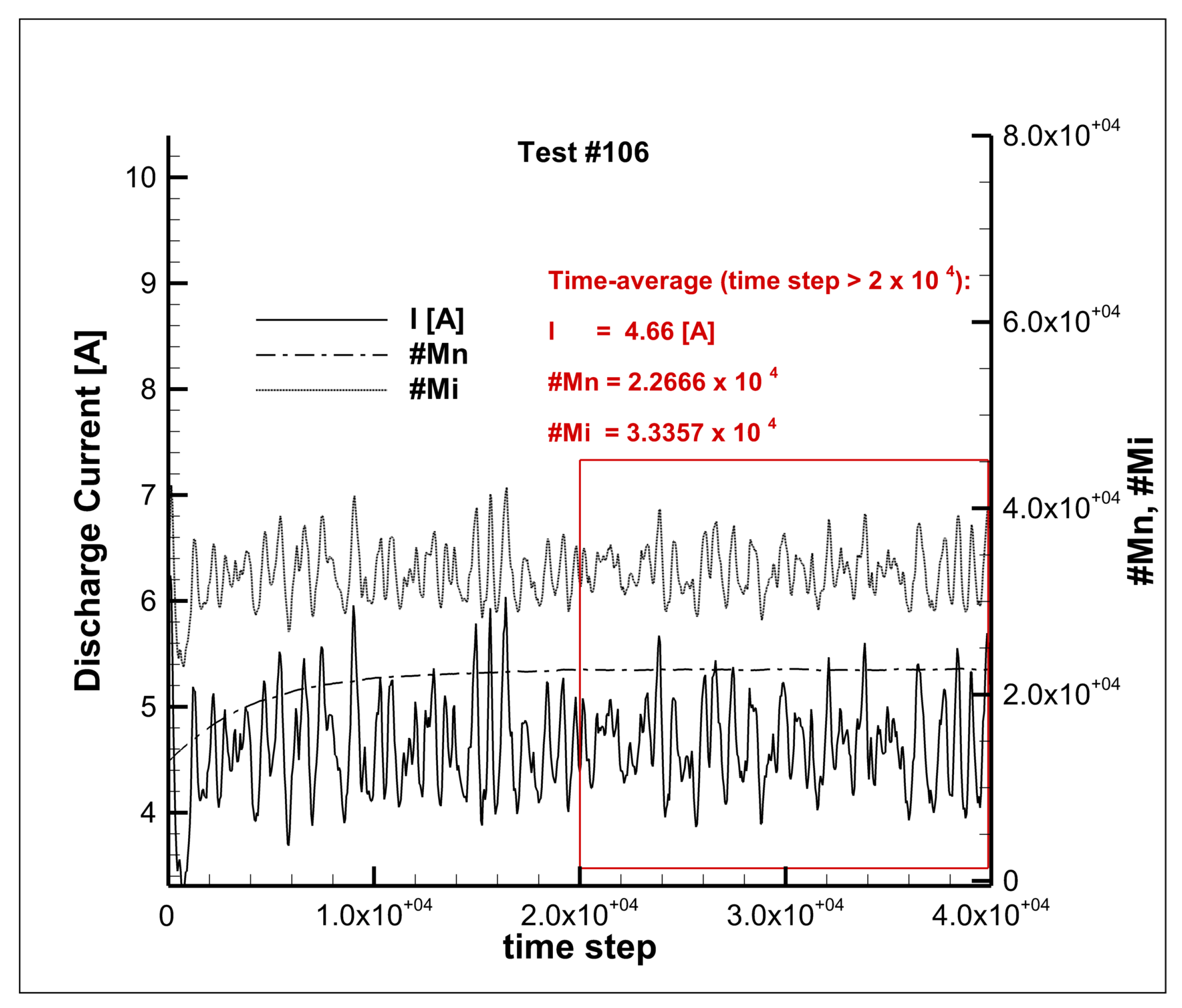
The number of followed heavy particles (neutrals and ions) and discharge current are selected as global parameters to monitor the simulation and to decide when to stop the calculation. Figure 11 shows these parameters as a function of time step number for Test 106. The sampling frequency is 50 time steps.
Table 3 reports time-averaged values of neutral/ion macro-particle number, discharge current and average number of macro-particle per cell (obtained by dividing the number of simulated particles with the total cell numbers). The averages were performed after 20 k time steps.
The selected specific weights of neutral and ion macro-particles allow to get averaged numbers of macro-particles per cell higher than 30, as required to smooth numerical oscillation due to the PIC method. It is also possible to observe that the discharge current seems to converge to the expected value of 4.5 A (Table 1).
4.2.4. Mass Balance
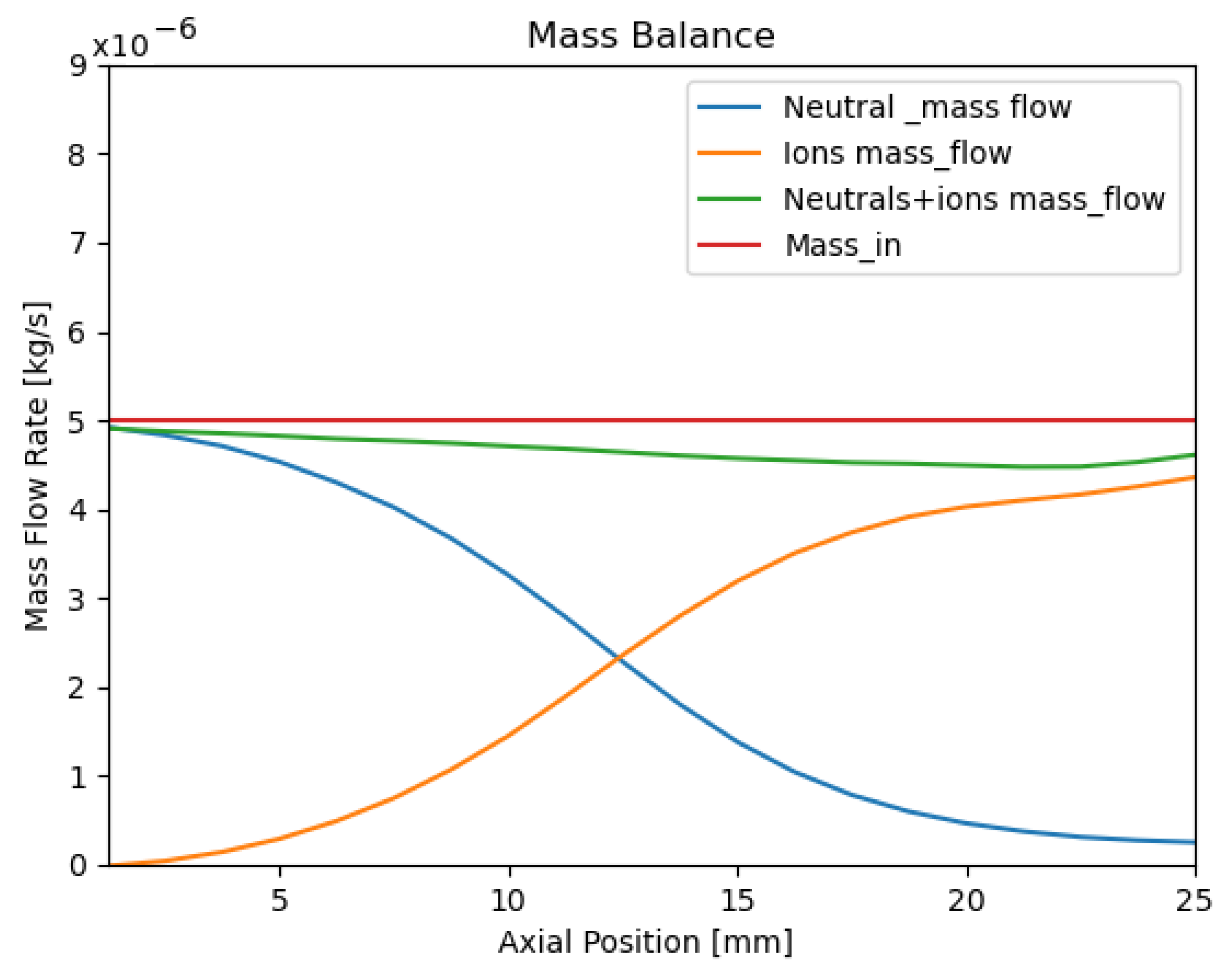
Mass conservation is verified. It is a very important check because the functions that creates ions and eliminates neutrals due to ionization are different. The trends of time-average ion mass flow and neutral mass flow are reported in Figure 12: the first increases toward the exit channel while the second decreases, as expected. Within the channel, at any section, the sum of mass flows must be as close as possible to inlet mass flow. The value are computed averaging solutions spaced by 50 time steps in the quasi steady-state regime.
4.3. Results Analysis
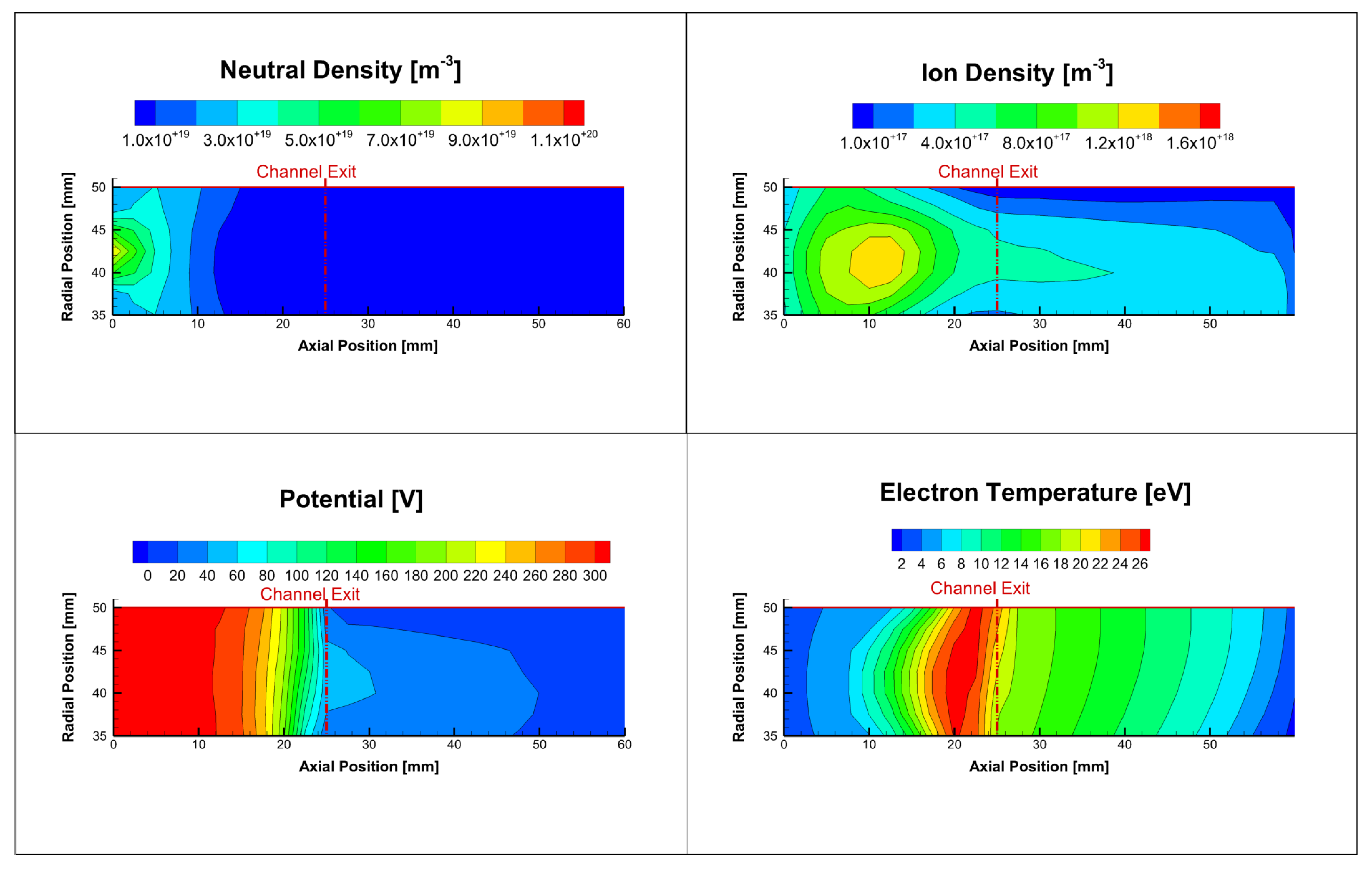
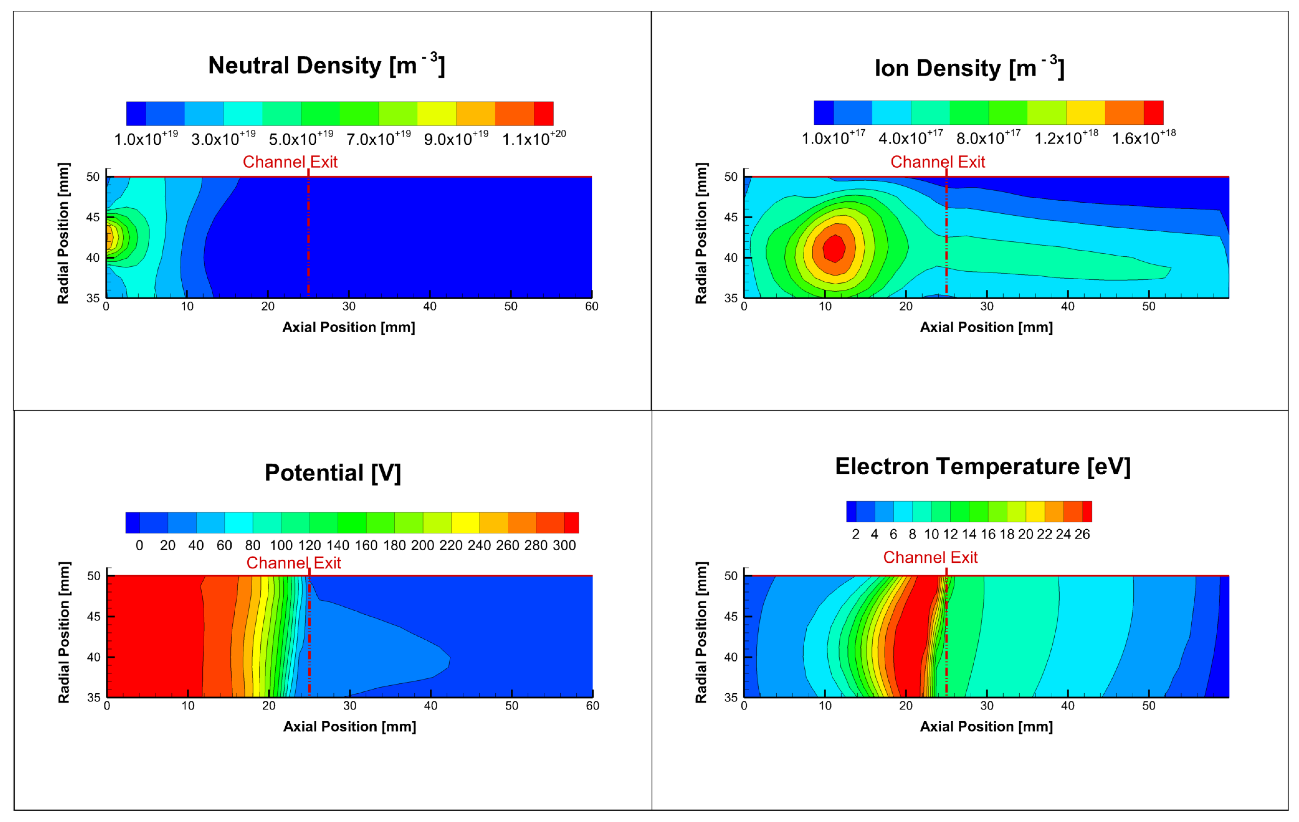
Figure 13 and Figure 14 show the time-averaged contour plots of the variables typically used to represents HET discharge. Qualitatively, the plasma physics described by the plots matches what is expected: neutrals expand within the channel; plasma potential sharply decays at channel’s exit where electron temperature reaches its maximum value; maximum ion density is just upward the exit section of channel and ions move downstream at high speed (order of thousand of km/s) because of the electric field.
The effect of grid refinement is clearly visible:
- Neutral density contour plots are better characterized, particularly near the anode;
- Ion peak tends to increase its value and the field is overall less diffused with respect to the computation with coarse grid, e.g., the plume is better defined;
- Electron temperature decreases more sharply.
The results of Figure 14 are compared to those reported by Hofer et al. [17] who use the code HPHall2 [16] disabling double-charge ion species creation. It is possible to observe that:
- The peak of electron temperature computed by HYPICFLU is slightly higher than that predicted by HPHall2;
- Plasma potential profile in the wall sheath drops very smoothly with respect to HPHall2, due to a different sheath model; this would affect ion velocities toward the wall and consequently its erosion;
- Ion density field is more diffused in the channel and the peak is higher; refining the grid, diffusion could be further lowered; there is a small deviation of ion plume toward the axis, probably due to the magnetic field configuration.
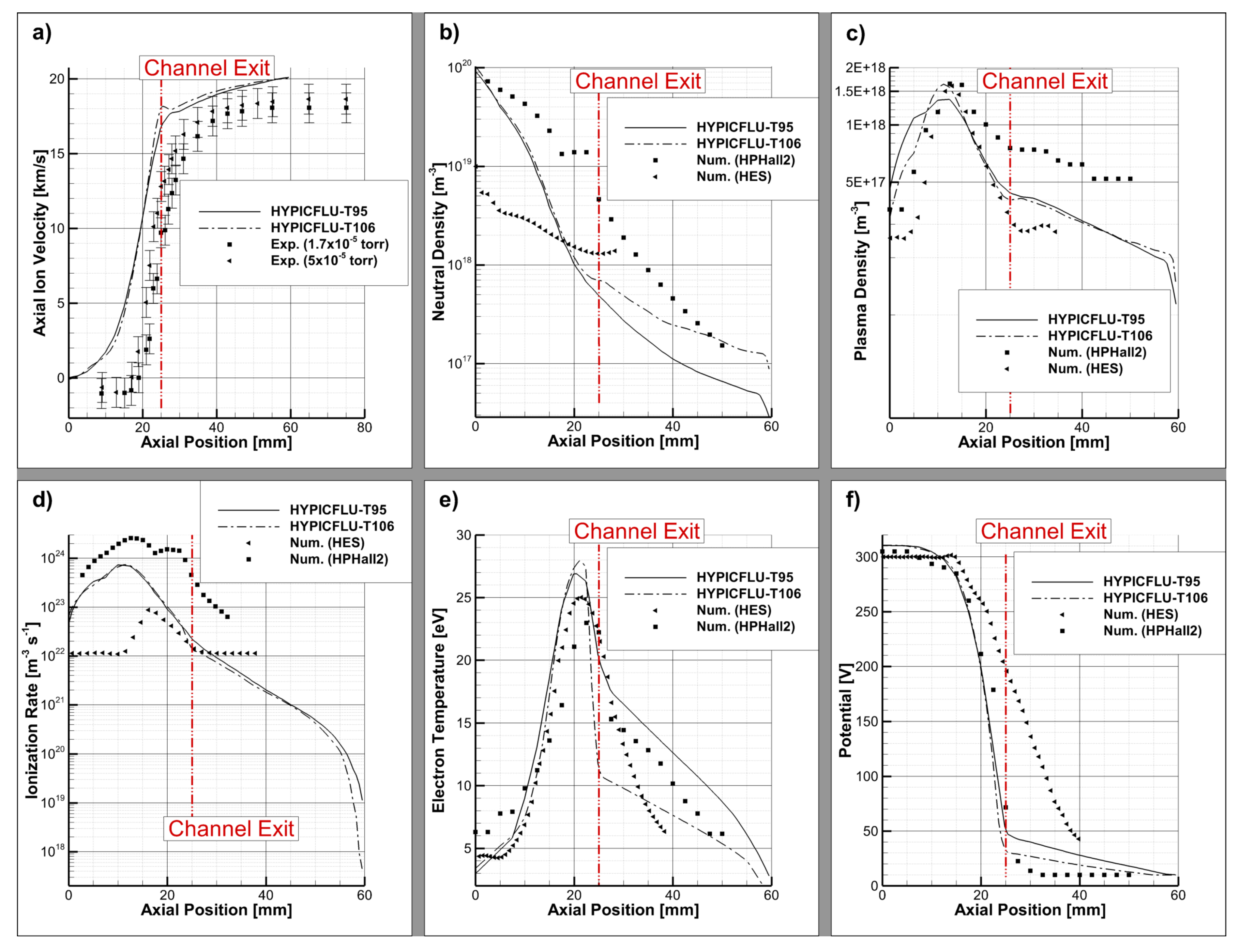
The values along channel centreline (radial position = 42.5 mm) are extracted from the solution domain and compared to the data presented by Hofer et al. [17] (HPHall2 code) and Kawashima et al. [28] (Hyperbolic-Equation System, HES, approach for the computation of magnetized electron fluids, proposed by Komurasaki and Akarawa [14]), Figure 15. Axial ion velocities computed by HYPICFLU are compared to the experimental measurements by means of Laser-Induced Fluorescence (LIF) velocimetry [36], measured at two facility background pressures ( and torr).
Neutral density (Figure 15b) at the inlet ( m) is very similar with the values computed by HPHall2. The value predicted with the HES approach is one order of magnitude less; the expansion trends are similar but the slopes of HYPICFLU curves are a little higher than HPHall2s (i.e., neutral density at exit channel is about m vs. m).
The electron temperature peaks are over-predicted by ∼2 eV with respect to both reference codes (Figure 15e). Within the channel, the electron temperatures coincides, but outside, in the plume region, the decay trends differ. As seen above, grid refinement leads to sharper decrease of electron temperature. It has been found that varying Bohm constant (), it is possible to change the slope of curves: lower values lead to a reduction of temperatures’ decay.
The peak of plasma density, located 10 mm downstream the anode, is ∼ m, matching both HPHall2 and HES predicted values (Figure 15c). After the peak, ion density decays quite rapidly with respect to HPHall2, but similarly to the HES approach; this is attributed to boundary condition effects.
The decay of potential in Test 95 (Figure 15f) well matches HPHall2 data, predicting a maximum electric field of ∼30 kV m. The main difference is in the plume where potential decreases more slowly. Grid refinement leads to higher slope at the exit section (axial electric peak in Test 106 is about ∼40 kV m) but outside the channel potential curve is closer to the HPHall2 one. It is verified that trigging Bohm constants, , it could be possible to modify plasma potential trends as well as, as seen above, electron temperature profiles.
Axial ion velocities computed by HYPICFLU (Figure 15a) continuously increase in the channel, as expected, but values are over-predicted with respect to the experimental data. Adjusting anomalous mobility parameters, it could be possible to reduce differences as shown by Adam et al. [22].
Ionization rates are compared in Figure 15d. HYPICFLU curves are below HPHall2 ones and they have weaker peaks ( vs. m s). It is mostly due to the higher neutral expansion and partially (i.e., within the channel) due to ion expansion after the peak.
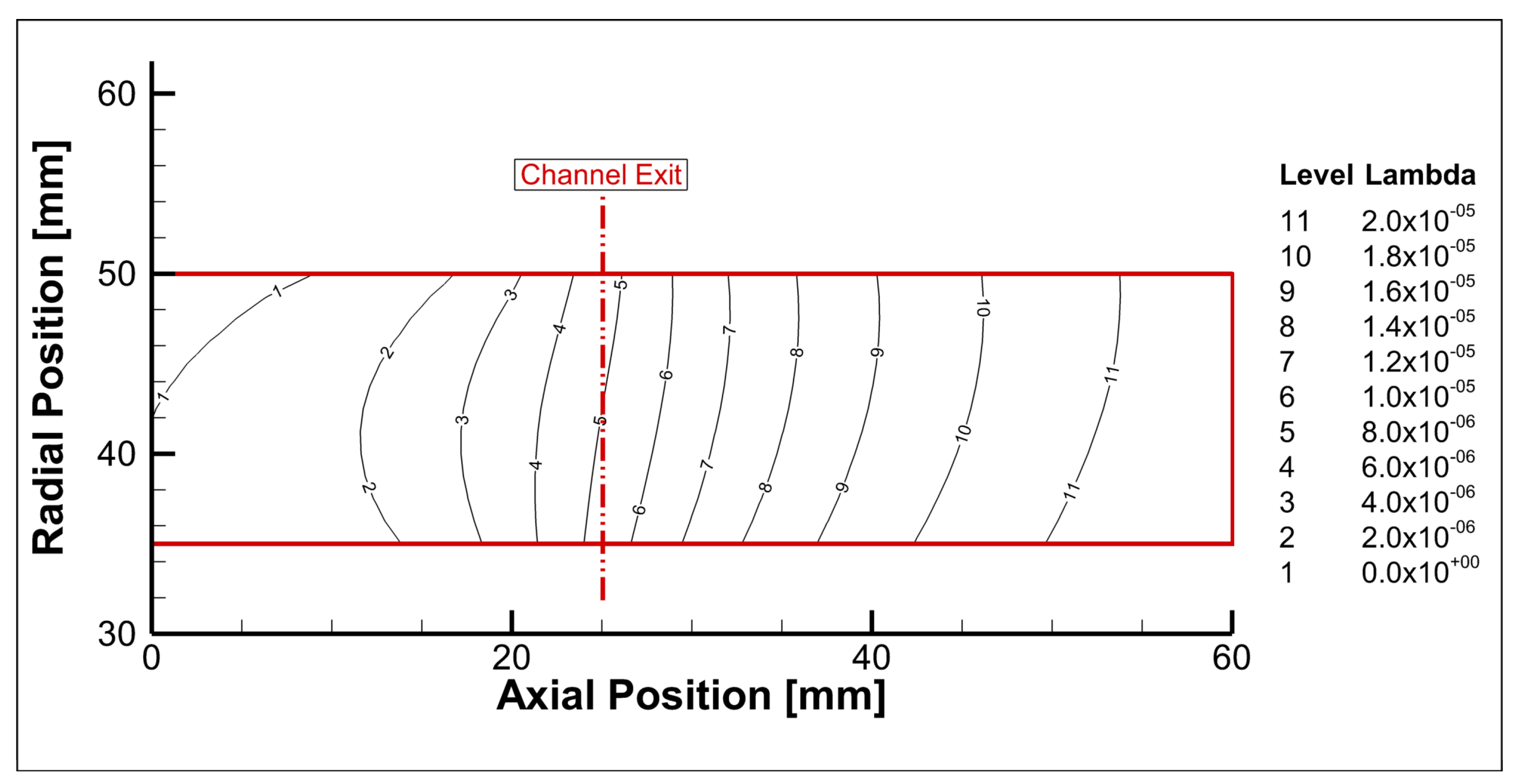
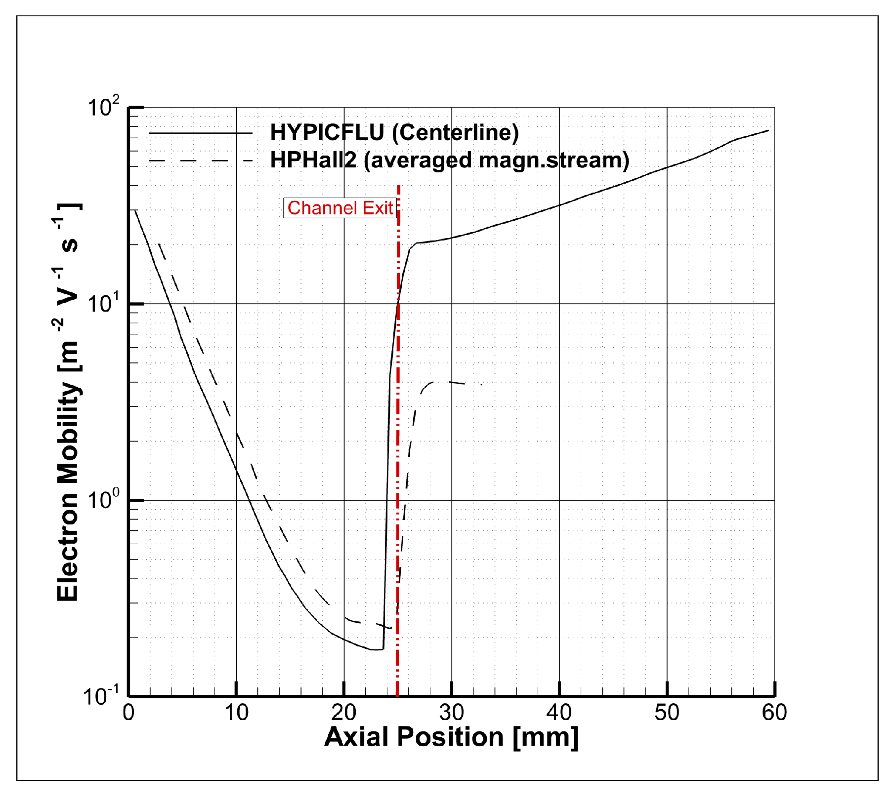
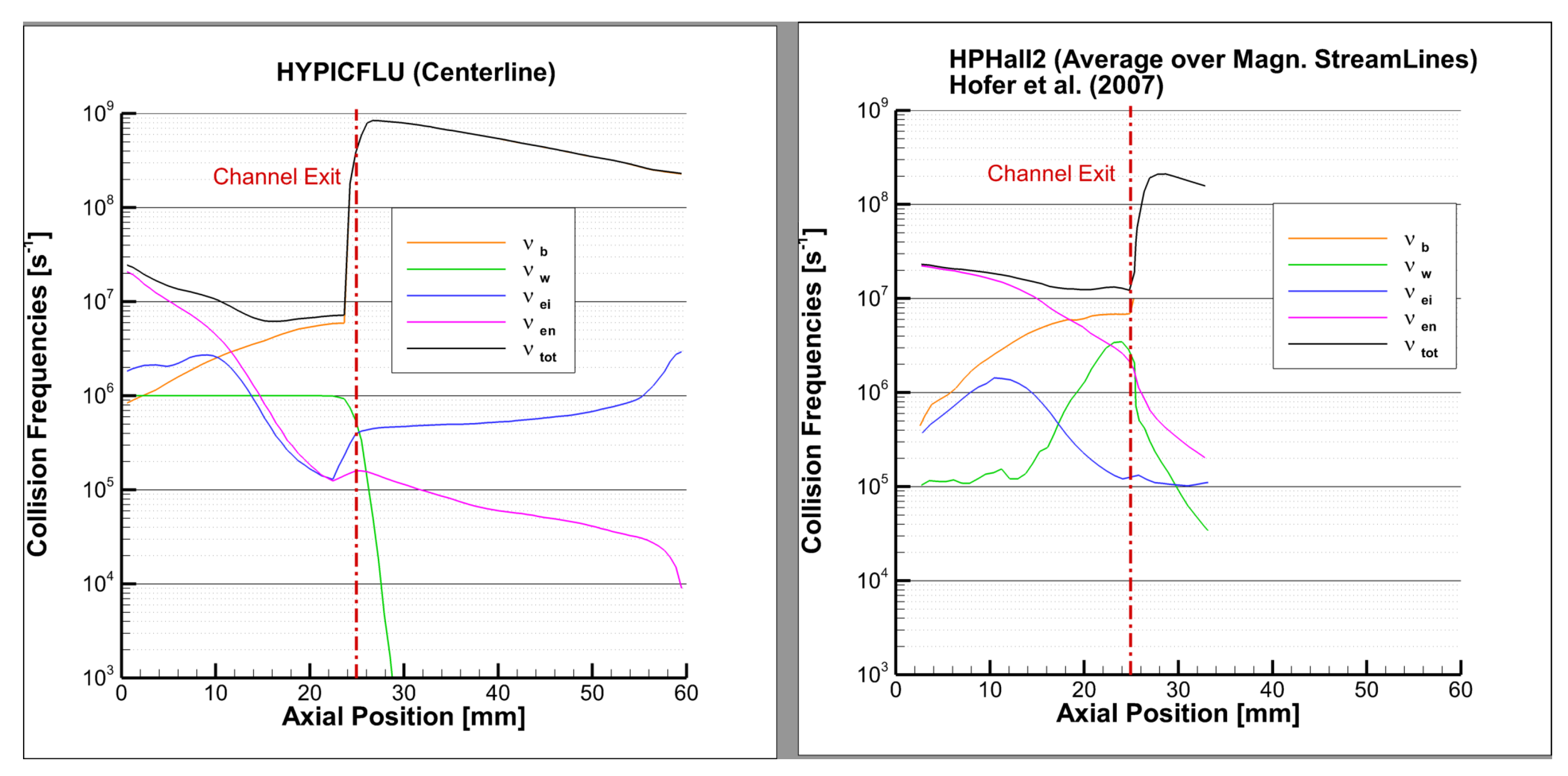
Figure 16 shows the electron mobility as a function of axial position. The main difference was outside the channel, where two different values of Bohm constant, , were used (HPHall: 1; HYPICFLU: 5). It is worth noting that HYPICFLU used a simpler wall collision frequency model [18] than HPHall2 and a formula [29] that fit the most recent electron–neutral cross-section for Xenon (thus, affecting directly electron–neutral collision frequency), Figure 17. The electron–ion collision frequency instead is affected by the differences between ion density and electron temperature profiles along channel centreline.
4.3.1. Performance
Thruster performances predicted by the code, compared to numerical and experimental data, are reported in Table 4. They are computed according to the classical formulas [1]:
Here, and are the mean ion velocity and mass flow rate at the cathode line. g is the gravitational constant at Earth’s surface. Thruster efficiency, , is defined as the thrust, T, times the exhaust velocity, , divided by the total input power, . From the definition of specific impulse, , and thrust, it is possible to easily get Equation (32).
Ions’ exhaust velocity at the cathode line is over-predicted; thus, the specific impulse is too. Ion mass flow rate is under-predicted. Consequently, thrust level, being the product between velocity and mass flow rate, is always matched. Thrust efficiency is slightly higher than both numerical and experimental values.
4.3.2. Computing Cost
Here we report some brief considerations on computing cost. About 70% of the computing cost depends on total number of simulated macro-particles, the remaining 30% on integration of electron equations. The operations are sequentially executed on Intel(R) Xeon(R) CPU E5-2640 v4 @ 2.40 GHz. As a result that the primary goal of the study was to test the model, no care was taken in reducing computational time of the code. Table 5 reports for each test the number of time step per hour, the total number of time steps and total computational time.
5. Conclusions
In this paper, we have described a newly developed code (HYPICFLU) for Hall Thruster plasma modelling. The code implements a model that simulates the temporal and spatial behaviour of Hall Effect Thrusters’ plasma, both inside the accelerating channel and in the near-plume region, by means of a hybrid approach, Particle-In-Cell (PIC) for heavy species (neutral and ions) and fluid for electrons. A two-region electron mobility model has been incorporated, the “anomalous” part of which uses empirical constants that can vary as a continuous function of axial coordinates, respectively and k, for electron–wall collision frequency and Bohm diffusion/SEE effects. This model has the advantage of including recent developed relations for each relevant phenomena and therefore improving the overall reliability of modelling the plasma behaviour.
In order to verify these aspects, as a cornerstone test, the discharge of SPT-100 has been selected due to the availability of reliable numerical and experimental data. The simulation results seem to be quite in line with experimental data confirming that such a developed model catches the relevant phenomena in Hall Thrusters. The code–code comparison with HPHall2, the NASA-JPL hybrid-code, has shown that HYPICFLU shows a more diffusive behaviour in the plume region, where ions expand more rapidly (in contrast with experimental measurements, too) and that potential decay in the sheath is weaker, affecting ion-to-wall velocity. The best fit of numerical and experimental data has been obtained by using a = 0.1, k = 0.035 inside the channel and k = 5 outside; the outer value of k is higher than the value used by HPHall-2 whereas the inner one is the same set in HPHall-2 simulations. This aspect is interesting and it is worth it to be further explored. The possible causes of over-expansion could be addressed first by the instance to the effect of mobility function’s shape (i.e., by changing k values and how rapidly the curves vary from inner to outer region) and secondly to the effect of near-plume geometry (i.e., by using semicircular area, like the most of codes). These aspects will be the object of future investigations and by means of the experimental testing that will be conducted on the low-power HET developed in CIRA [42].
Other future developments of the model will include the implementation of a more detailed wall sheath model, aimed to better predict ion velocity for wall to wall erosion calculation; the use of the same grid for PIC and fluid modules, built from the magnetic streamlines, in order to avoid interpolation errors. As a result of the high computational cost, an optimization of the code, to increase the convergence speed, is also foreseen.
In the near future, a parametric study to investigate other operative conditions of SPT-100 will be conducted to asses how the mobility parameters have to be changed to match the expected performances and to further assess the code.
Author Contributions
Conceptualization, M.P. and F.B.; methodology, D.M. and M.P.; software, M.P., B.M., F.A.D. and D.M.; validation, M.P., B.M., F.A.D. and D.M.; formal analysis, B.M. and F.A.D.; data curation, M.P.; writing—original draft preparation, M.P.; writing—review and editing, F.B.; visualization, M.P.; supervision, M.P.; project administration, F.B. All authors have read and agreed to the published version of the manuscript.
Funding
This research was funded by the Italian research program in aerospace, PRORA (Programma Operativo Ricerche Aerospaziali) entrusted by MIUR (Ministero dell’Istruzione, Ministero dell’Università e della Ricerca).
Institutional Review Board Statement
Not applicable.
Informed Consent Statement
Not applicable.
Data Availability Statement
The data presented in this study are available on request from the corresponding author.
Acknowledgments
The authors would like to thank all people involved in the MEMS project and F. Nasuti (University of Rome, La Sapienza), E. Martelli (University of Campania, L. Vanvitelli) and R. Savino (University of Naples, Federico II) who entrusted their graduated students (respectively D.M., F.A.D and B.M.) to the CIRA space propulsion laboratory, giving them the possibility to contribute to this study.
Conflicts of Interest
The authors declare no conflict of interest.
Abbreviations
The following symbols, subscripts and abbreviations are used in this manuscript:
| Symbols | |
| Boltzmann constant | |
| e | Electron charge |
| Electron mass | |
| Ion mass | |
| Dielectric constant of the free space | |
| Magnetic permeability of the free space | |
| t | time |
| r | Radial coordinate |
| z | Axial coordinate |
| I | Current |
| Electric field | |
| Magnetic field | |
| n | Particle number density |
| Velocity vector | |
| Electron temperature | |
| Ionization rate | |
| Potential | |
| Thermalized potential | |
| Magnetic streamline | |
| current density vector | |
| V | Volume/Voltage |
| Electron mobility | |
| Collision frequency | |
| Heat conduction due to electrons | |
| Heat conduction coefficient | |
| Elastic-inelastic source terms | |
| Joule heating source term | |
| Ionization energy | |
| Excitation Cross section ground to | |
| Cross section of ground state ionization | |
| Ion production cost | |
| Normalized ion production cost | |
| Electron mean thermal speed | |
| Flux of electrons | |
| SEE yield | |
| Ionization coefficient | |
| q | Energy flux to the wall |
| Subscripts | |
| tangent to magnetic streamline | |
| normal to magnetic streamline | |
| i | ion |
| e | electron |
| n | neutral |
| w | wall |
| electron–neutral | |
| electron–ion | |
| b | Bohm |
| a | anode |
| c | cathode |
| d | discharge |
| break-up | |
| secondary electrons emitted | |
| Abbreviations | |
| HET(s) | Hall Effect Thruster(s) |
| SPT | Stationary Plasma Thruster |
| PIC | Particle-In-Cell |
| HYPICFLU | HYbrid PIC-FLUid |
| FVM | Finite Volume Method |
| MS(s) | Magnetic Streamline(s) |
| RHS | Right Hand Side |
| SEE | Secondary Electron Emission |
| BC | Boundary Condition |
| CEX | Charge Exchange |
| MCC | Monte Carlo Collision |
| VDF | Velocity Distribution Function |
| FVM | Finite Volume Method |
| LIF | Laser-Induced Fluorescence |
Appendix A. Magnetic Stream Function
The magnetic field, , and its evolution are governed by the Maxwell’s equations:
Here, is the current density, is the electric field vector while and are respectively the dielectric constant and the magnetic permeability of the free space. However, the RHS of Equation (A2) can be neglected [13], resulting in:
This means that the magnetic field it is not influenced by the motion of the charged particles and it is determined only by the magnetic circuit of the thruster, in other words is static. It is therefore possible to define a magnetic stream function which relates with the cylindrical components of the magnetic field (, ) by:
The gradient of this stream function is orthogonal to and it is related with the strength of the magnetic field. Therefore, the gradient of is:
This allows to rewrite the derivatives along the normal of the magnetic field lines, , as derivatives with respect of :
As a stream function, must satisfy the Laplace equation that can be rewritten in cylindrical coordinates as follows:
Appendix B. Integrals’ Factors
In the following, all of the factors used in the discrete form of current conservation (Equation (11)) and the electron energy equation (Equation (12)) are reported. It is worth to remember that for quasi-neutrality . The indices, k, denote the nodes that discretize the magnetic streamlines ().
where , , , , are respectively the interpolated electron density, ion velocity and mobility normal to magnetic streamline, magnetic field intensity, radial coordinate and the surface associated to the node k.
where and are respectively the interpolated ionization rate and the volume associated to the node k.
Here, the sum is performed on the points that discretize the magnetic field line associated with the surfaces () or () and each point k has an associated , and , where:
Again, the summation is performed as specified above and , r[k] and are respectively the magnetic field, the radial coordinate and the modified heat conduction coefficient (i.e., ) calculated or interpolated at the point k.
Here, the sum is performed over the magnetic streamline associated with the volume element .
References
- Goebel, D.M.; Katz, I. Fundamentals of Electric Propulsion: Ion and Hall Thrusters; Wiley: Hoboken, NJ, USA, 2008. [Google Scholar]
- Boeuf, J. Tutorial: Physics and modeling of Hall thrusters. J. Appl. Phys. 2017, 121, 011101. [Google Scholar] [CrossRef]
- Adam, J.C.; Héron, A.; Laval, G. Study of stationary plasma thrusters using two dimensional fully kinetic simulations. Phys. Plasmas 2004, 11, 295–305. [Google Scholar] [CrossRef]
- Sydorenko, D.; Smolyakov, A.; Kaganovich, I.; Raitses, Y. Kinetic simulation of effects of secondary electron emission on electron temperature in hall thrusters. In Proceedings of the 29th Annual International Electric Propulsion Conference, Princeton, NJ, USA, 31 October–4 November 2005. IEPC-2005-078. [Google Scholar]
- Tskhakaya, D.; Matyash, K.; Schneider, R.; Taccogna, F. The particle-in-cell method. CPP 2007, 47, 563–594. [Google Scholar] [CrossRef]
- Coche, P.; Garrigues, L. Study of stochastic effects in a hall effect thruster using a test particles monte-carlo model. In Proceedings of the 32nd International Electric Propulsion Conference, Wiesbaden, Germany, 11–15 September 2011. IEPC-2011-255. [Google Scholar]
- Cho, S.; Watanabe, H.; Kubota, K.; Iihara, S.; Fuchigami, K.; Uematsu, K.; Funaki, I. Study of electron transport in a Hall thruster by axial-radial fully kinetic particle simulation. Phys. Plasmas 2015, 22, 103523. [Google Scholar] [CrossRef]
- Croes, V.; Tavant, A.; Lucken, R.; Lafleur, T.; Bourdon, A.; Chabert, P. Study of electron transport in a hall effect thruster with 2d r-θ particle-in-cell simulations. In Proceedings of the 35th International Electric Propulsion Conference, Atlanta, GA, USA, 8–12 October 2017. [Google Scholar]
- Ahedo, E.; Martinez-Cerezo, P.; Martinez-Sanchez, M. One-Dimensional Model of the Plasma Flow in a Hall Thruster. Phys. Plasmas 2001, 8, 3058–3068. [Google Scholar] [CrossRef]
- Keidar, M.; Boyd, I.D.; Beilis, I.I. Plasma Flow and Plasma-Wall Transition in Hall Thruster Channel. Phys. Plasmas 2002, 9, 5315–5322. [Google Scholar] [CrossRef] [Green Version]
- Roy, S.; Pandey, B.P. Development of a finite element based Hall thruster model for Sputter Yield Prediction. In Proceedings of the 27th International Electric Propulsion Conference, Pasadena, CA, USA, 8–12 October 2001. IEPC-2001-049. [Google Scholar]
- Fife, J.M. Two-Dimensional Particle-In-Cell Modelling of Hall Thrusters. Master’s Thesis, Massachusetts Institute of Technology, Cambridge, MA, USA, May 1995. [Google Scholar]
- Fife, J.M. Hybrid-PIC Modeling and Electrostatic Probe Survey of Hall Thrusters. Ph.D. Thesis, Massachusetts Institute of Technology, Cambridge, MA, USA, September 1998. [Google Scholar]
- Komurasaki, K.; Arakawa, Y. Two-dimensional numerical model of plasma flow in a hall thruster. J. Propuls. Power 1995, 11, 1317–1323. [Google Scholar] [CrossRef]
- Escobar, D.; Ahedo, E. Two-dimensional electron model for a hybrid code of a two-stage Hall thruster. IEEE Trans. Plasma Sci. 2008, 36, 2043–2057. [Google Scholar] [CrossRef] [Green Version]
- Hofer, R.R.; Katz, I.; Mikellides, I.; Gamero-Castano, M. Heavy Particle Velocity and Electron Mobility Modeling in Hybrid-PIC Hall Thruster Simulations. In Proceedings of the 42nd AIAA/ASME/SAE/ASEE Joint Propulsion Conference & Exhibit, Sacramento, CA, USA, 9–12 July 2006. AIAA 2006-4658. [Google Scholar]
- Hofer, R.R.; Mikellides, I.G.; Katz, I.; Goebel, D.M. Wall Sheath and Electron Mobility Modeling in Hybrid-PIC Hall Thruster Simulations. In Proceedings of the 43rd AIAA/ASME/SAE/ASEE Joint Propulsion Conference and Exhibit, Cincinnati, OH, USA, 8–11 July 2007. AIAA 2007-5267. [Google Scholar]
- Hagelaar, G.J.M.; Bareilles, J.; Garrigues, L.; Boeuf, J.P. Two-dimensional model of a stationary plasma thruster. J. Appl. Phys. 2002, 91, 5592. [Google Scholar] [CrossRef]
- Koo, J.W. Hybrid PIC-MCC Computational Modeling of Hall Thrusters. Ph.D. Thesis, The University of Michigan, Ann Arbor, MI, USA, 2005. [Google Scholar]
- Raisanen, A.L.; Hara, K.; Boyd, I.D. Two-dimensional hybrid-direct kinetic simulation of a Hall thruster discharge plasma. Phys. Plasmas 2019, 26, 123515. [Google Scholar] [CrossRef]
- Bishaev, A.; Kim, V. Local Plasma Properties in a Hall-Current Accelerator with an Extended Acceleration Zone. Sov. Phys. Tech. Phys. 1978, 23, 1055–1057. [Google Scholar]
- Adam, J.C.; Boeuf, J.P.; Dubuit, N.; Dudeck, M.; Garrigues, L.; Gresillon, D.; Heron, A.; Hagelaar, G.J.M.; Kulaev, V.; Lemoine, N.; et al. Physics, simulation and diagnostics of Hall effect thrusters. Plasma Phys. Control. Fusion 2008, 50, 124041. [Google Scholar] [CrossRef]
- Hofer, R.; Katz, I.; Goebel, D.; Jameson, K.; Sullivan, R.; Johnson, L.; Mikellides, I. Efficacy of Electron Mobility Models in Hybrid-PIC Hall Thruster Simulations. In Proceedings of the 44th AIAA/ASME/SAE/ASEE Joint Propulsion Conference and Exhibit, Hartford, CT, USA, 21–23 July 2008. AIAA 2008-4924. [Google Scholar]
- Parra, F.I.; Ahedo, E.; Fife, J.M.; Martinez-Sanchez, M. A two-dimensional hybrid model of the Hall thruster discharge. J. Appl. Phys. 2006, 100, 023304. [Google Scholar] [CrossRef]
- Morozov, A.I.; Esinchuk, Y.V.; Tilinin, G.N. Plasma Accelerator With Closed Electron Drift And Extended Acceleration Zone. Sov. Phys. Tech. Phys. (Engl. Transl.) 1972, 17, 38–45. [Google Scholar]
- Huba, J.D. NRL Plasma Formulary; Naval Research Laboratory: Washington, DC, USA, 2007. [Google Scholar]
- Nickel, J.C.; Imre, K.; Register, D.F.; Trajmar, S. Total Electron Scattering Cross Sections: I. He, Ne, Ar, Xe. J. Phys. At. Mol. Opt. Phys. 1985, 18, 125–133. [Google Scholar] [CrossRef]
- Kawashima, R.; Komurasaki, K.; Schonherr, T.; Koizumi, H. Hybrid Modeling of a Hall Thruster Using Hyperbolic System of Electron Conservation Laws. In Proceedings of the 34th International Electric Propulsion Conference, Hyogo-Kobe, Japan, 4–10 July 2015. IEPC-2015-206. [Google Scholar]
- Panelli, M.; Giaquinto, C.; Smoraldi, A.; Battista, F. A Plasma Model for Orificed Hollow Cathode. In Proceedings of the 36th International Electric Propulsion Conference, University of Vienna, Austria, Vienna, 15–20 September 2019. [Google Scholar]
- Arhipov, B.; Krochak, L.; Kudriavcev, S.; Murashko, V.; Randolph, T. Investigation of the Stationary Plasma Thruster (SPT-100) Characteristics and Thermal Maps at the Raised Discharge Power. In Proceedings of the 34th AIAA/ASME/SAE/ASEE Joint Propulsion Conference, Cleveland, OH, USA, 13–15 July 1998. AIAA 98-3791. [Google Scholar]
- Birdsall, C.L.; Langdon, A.B. Plasma Physics via Computer Simulation; Adam Hilger; Institute of Physics Publishing: Bristol, UK; Philadelphia, PA, USA; New York, NY, USA, 1991. [Google Scholar]
- Dugan, J.V., Jr.; Sovie, R.J. Volume Ion Production Costs in Tenuous Plasmas: A General Atom Theory and Detailed Results for Helium, Argon and Cesium; National Aeronautics and Space Administration: Washington, DC, USA, 1967; NASA-TN-D-4150. [Google Scholar]
- Alvarez, C.A.; HRiascos, H.; Gonzalez, C. 2D electrostatic PIC algorithm for laser induced studying plasma in vacuum. J. Phys. Conf. Ser. 2016, 687, 012072. [Google Scholar] [CrossRef] [Green Version]
- Particle-In Cell Consulting. Available online: https://www.particleincell.com/2015/rz-pic/ (accessed on 28 May 2021).
- The Electrostatic Particle In Cell (ES-PIC) Method. Available online: https://www.particleincell.com/2010/es-pic-method (accessed on 20 April 2021).
- Macdonald, N.; Pratt, Q.; Nakles, M.; Pilgram, N.; Holmes, M.; Hargus, W. Background Pressure Effects on Ion Velocity Distributions in an SPT-100 Hall Thruster. J. Propuls. Power 2019, 35, 1–10. [Google Scholar] [CrossRef] [Green Version]
- Kybeom, K. A Novel Numerical Analysis of Hall Effect Thruster and Its Application in Simultaneous Design of Thruster and Optimal Low-Thrust Trajectory. Ph.D. Thesis, Georgia Institute of Technology, Atlanta, GA, USA, August 2010. [Google Scholar]
- Racca, G.D.; Foing, B.H.; Coradini, M. SMART-1: The First Time of Europe to the Moon; Barbieri, C., Rampazzi, F., Eds.; Earth-Moon Relationships; Springer: Dordrecht, The Netherlands, 2001. [Google Scholar]
- SPT-100. Available online: http://www.astronautix.com/s/spt-100.html (accessed on 20 April 2021).
- Sankovic, J.M.; Hamley, J.A.; Haaa, T.W. Performance Evaluation of the Russian SPT-100 Thruster at NASA LeRC. In Proceedings of the 23rd International Electric Propulsion Conference, Seattle, WA, USA, 13–16 September 1993. IEPC-93-094. [Google Scholar]
- Finite Element Method Magnetics (FEMM). Available online: http://www.femm.info/wiki/HomePage (accessed on 20 April 2021).
- Invigorito, M.; Ricci, D.; Battista, F.; Smoraldi, A.; Panelli, M.; Salvatore, V. Activities on Electric Space Propulsion at Italian Aerospace Research Centre: Main Achievements And Outlook. In Proceedings of the 6th ESA Space Propulsion Conference, Seville, Spain, 14–18 May 2018. [Google Scholar]
Figure 1.
A scheme illustrating a Hall Effect Thruster and its principles of functioning.

Figure 2.
HYPICFLU: variables exchange between fluid and PIC sub-models.

Figure 3.
Flow chart of the HYPICFLU code. Typical integration time-steps are reported.

Figure 4.
(a) Volume element for the FVM approach to solve the electron energy equation; (b) nodes on a magnetic streamline and example of an associated volume () used in the integration of factors; (c) integration surfaces of a fluid element.
Figure 4.
(a) Volume element for the FVM approach to solve the electron energy equation; (b) nodes on a magnetic streamline and example of an associated volume () used in the integration of factors; (c) integration surfaces of a fluid element.

Figure 5.
Picture of SPT-100 [39].
Figure 5.
Picture of SPT-100 [39].

Figure 6.
SPT-100 performance: specific impulse and thruster efficiency as function of power(Data from Ref. [40]). The design point is selected in the present study.
Figure 6.
SPT-100 performance: specific impulse and thruster efficiency as function of power(Data from Ref. [40]). The design point is selected in the present study.

Figure 7.
PIC (49 × 13) and fluid meshes (42 × 13). Blue line denotes the anodic inlet of Xenon particles.
Figure 7.
PIC (49 × 13) and fluid meshes (42 × 13). Blue line denotes the anodic inlet of Xenon particles.

Figure 8.
SPT-100: magnetic field intensity calculated by FEMM and interpolated on the PIC grid (25 × 7). Dash-dot red line denotes channel exit whereas the continuous red line indicates the channel centreline.
Figure 8.
SPT-100: magnetic field intensity calculated by FEMM and interpolated on the PIC grid (25 × 7). Dash-dot red line denotes channel exit whereas the continuous red line indicates the channel centreline.

Figure 9.
SPT-100 radial magnetic field intensity, along the channel centreline, as a function of axial position (z) compared to reconstructed data from Hofer et al. [17].
Figure 9.
SPT-100 radial magnetic field intensity, along the channel centreline, as a function of axial position (z) compared to reconstructed data from Hofer et al. [17].

Figure 10.
SPT-100: magnetic stream function () computed from magnetic field.

Figure 11.
Test 106 Number of followed heavy particles (neutrals, Mn and ions, Mi) and discharge current as a function of time step number. Sampling: 50 time steps. Time step: s.
Figure 11.
Test 106 Number of followed heavy particles (neutrals, Mn and ions, Mi) and discharge current as a function of time step number. Sampling: 50 time steps. Time step: s.

Figure 12.
Test 106 Mass balance within the accelerating channel.

Figure 13.
SPT-100 simulation: Test 95. Time-averaged contour plots of neutral and plasma densities, potential and electron temperature. Average window: 1 ms.
Figure 13.
SPT-100 simulation: Test 95. Time-averaged contour plots of neutral and plasma densities, potential and electron temperature. Average window: 1 ms.

Figure 14.
SPT-100 simulation: Test 106. Time-averaged contour plots of neutral and plasma densities, potential and electron temperature. Average window: 1 ms.
Figure 14.
SPT-100 simulation: Test 106. Time-averaged contour plots of neutral and plasma densities, potential and electron temperature. Average window: 1 ms.

Figure 15.
SPT-100 simulation: (a) axial ion velocity, (b,c) neutral and plasma densities, (d) ionization rate, (e) electron temperature and (f) plasma potential as a function of axial position (along a line going through the middle of the channel). HYPICFLU-Test 95 and HYPICFLU-Test106 curves have been extracted from Figure 13 and Figure 14; experimental (Exp.) data have been taken from MacDonald-Tenenbaum et al. [36] and refer to two background pressure levels within the test chamber; numerical (Num.) results have been taken from Hofer et al. (using HPHall2 code) and Kawashima et al. (using HES-based code), respectively.

Figure 16.
SPT-100 discharge: time-averaged mobility as a function of axial position. Comparison between HYPICLFU (Test 106: data taken along channel centreline) and HPHall2(data averaged over magnetic streamlines, reconstructed from Ref. [17]).
Figure 16.
SPT-100 discharge: time-averaged mobility as a function of axial position. Comparison between HYPICLFU (Test 106: data taken along channel centreline) and HPHall2(data averaged over magnetic streamlines, reconstructed from Ref. [17]).

Figure 17.
SPT-100 discharge: time-averaged collision frequency contributing to mobility as a function of axial position. Comparison between HYPICLFU (Test 106: data taken along channel centreline) and HPHall2 [17] (data averaged over magnetic streamlines).
Figure 17.
SPT-100 discharge: time-averaged collision frequency contributing to mobility as a function of axial position. Comparison between HYPICLFU (Test 106: data taken along channel centreline) and HPHall2 [17] (data averaged over magnetic streamlines).


Table 1.
SPT-100: geometry and nominal operative parameters (data from [37]).
Table 1.
SPT-100: geometry and nominal operative parameters (data from [37]).
| Parameter | Value | Unit |
|---|---|---|
| Outer radius | 50 | mm |
| Inner radius | 35 | mm |
| Channel length | 25 | mm |
| Max. Radial Magnetic Intensity | 0.016 | T |
| Mass flow rate (Xe) | 5 | mg/s |
| Discharge Voltage | 300 | V |
| Discharge Current | 4.5 | A |
Table 2.
SPT-100: characteristics of discharge simulation tests.
| Test 95 | Test 106 | |
|---|---|---|
| PIC grid (nodes) | 25 × 7 | 49 × 13 |
| Cell dimensions (mm) | 0.25 | 0.125 |
| Fluid grid | 22 () × 7 (nodes) | 42 () × 13 (nodes) |
| Neutrals specific weigh | ||
| Ions specific weigh | ||
| Mobility-Bohm diffusion, | 0.035 | 0.035 |
| Mobility-Bohm diffusion, | 5 | 5 |
| Mobility elect-wall coll., | 0.1 | 0.1 |
| Anode temperature (K) | 750 | 750 |
| Walls temperature (K) | 850 | 850 |
| Cathode Potential (eV) | 10 | 10 |
| Cathode Electron Temperature (eV) | 4 | 4 |
Table 3.
SPT-100 discharge simulation: time-average discharge current and number of simulated macro-particles (neutrals and ions). The average numbers of particles per cell have been reported.
Table 3.
SPT-100 discharge simulation: time-average discharge current and number of simulated macro-particles (neutrals and ions). The average numbers of particles per cell have been reported.
| Test 95 | Test 106 | |
|---|---|---|
| Discharge current (A) | 4.8 | 4.66 |
| Simulated Ion particles (No.) | 10,700 | 33,357 |
| Ion particle (No.) per cell | 74 | 58 |
| Simulated Neutral particles (No.) | 6866 | 22,666 |
| Neutral particle (No.) per cell | 48 | 39 |
| Exp. | Num. | Test 95 | Test 106 | |
|---|---|---|---|---|
| (A) | 4.5 | 4.5 | 4.8 | 4.65 |
| (W) | 1350 | 1350 | 1440 | 1395 |
| (km/s) | 15.7 | 17.0 | 19.8 | 19.8 |
| (μg/s) | 5.29 | 5.00 | 3.93 | 4.19 |
| (s) | 1600 | 1733 | 2027 | 2016 |
| T (mN) | 83 | 85 | 78 | 83 |
| (%) | 50 | 55 | 58 | 59 |
Table 5.
SPT-100 discharge simulation: computational time.
| Test 95 | Test 106 | |
|---|---|---|
| Total Num. of macro-particles | 17,566 | 56,023 |
| Final time step | 46,650 | 40,000 |
| Time-to-final time step (days) | 5 | 16 |
| Time Step/hour | 294 | 116 |
Short Biography of Authors
Dr. Mario Panelli is a Sr. researcher in the force of space propulsion laboratory at the Italian Aerospace Research Centre (CIRA) since 2011. Mario received his Master of Science in Aerospace Engineering in 2007 at the University of Naples, Federico II. After graduation, he won a PhD scholarship in Aerospace, Naval and Quality Management Engineering at the same university that ended in 2011. Dr. Panelli gained experience in fluid-dynamic simulations dealing with a lot of topics (brake discs, cold jets, free convection) and in experimental measurements by means of kytoon station and IR thermography. He performed CFD simulations of several components of liquid-oxygen/methane rocket engines, paraffin-based hybrid rocket motors and pressure oscillations in solid rocket motors. His most recent activities are associated with space electric propulsion applications and they particularly include the design of Orifice Hollow Cathodes (OHCs) for low power Hall Effect Thrusters (HETs) and plasma modelling both for OHCs and HETs.
Mr. Davide Morfei is an aerospace engineer specialized in applications for space platforms. He received his Master of Science in Space and Astronautical Engineering at La Sapienza, University of Rome, in 2018. He had an internship at the Italian Aerospace Research Centre (CIRA) where he developed algorithms for the evaluation of plasma proprieties of Hall Effect Thrusters (HETs). He got a scholarship to CSU Electric Propulsion and Plasma Engineering (CEPPE) Laboratory in Denver (CO), USA. There, he took part in experimental characterization and development of HETs.
Mr. Beniamino Milo is an aerospace engineer specialized in software development for space propulsion applications. He graduated in Aerospace Engineering (Bachelor’s degree) at the University of Naples, Federico II, in 2017. He continued his study at the same university and he got his Master of Science in Aerospace Engineering in October 2020. As a graduate student, he was an intern at the Italian Aerospace Research Centre (CIRA) in the space propulsion laboratory where he contributed to the development of the particle-in-cell model for neutrals and ions in HETs’ plasma.
Mr. Francesco Antonio D’Aniello is an aerospace engineer specialized in space propulsion applications. He graduated in Aerospace Engineering (Bachelor’s degree) at the University of Campania, Luigi Vanvitelli, in October 2016. He continued his study at the same university and he got his Master of Science in Aerospace Engineering in November 2020. As a graduate student, he was an intern at the Italian Aerospace Research Centre (CIRA) in the space propulsion laboratory where he contributed to the development of a fluid model for electrons in HETs’ plasma.
Dr. Francesco Battista holds a PhD in Aerospace Engineering from the University of Pisa. He currently works in CIRA (Italian Aerospace Research Center), being affiliated with the Propulsion and Exploration Division responsible for the Space Propulsion Laboratory. He worked as a system engineer and project manager in different national and international projects mainly on the topics of methane-based propulsion systems, hybrid propulsion and electric propulsion. He is involved in the CIRA electric propulsion projects as the project manager and is technically responsible. He is the author or co-author of more than 100 papers, published in international journals and conference proceedings.
Publisher’s Note: MDPI stays neutral with regard to jurisdictional claims in published maps and institutional affiliations. |
© 2021 by the authors. Licensee MDPI, Basel, Switzerland. This article is an open access article distributed under the terms and conditions of the Creative Commons Attribution (CC BY) license (https://creativecommons.org/licenses/by/4.0/).
Share and Cite
MDPI and ACS Style
Panelli, M.; Morfei, D.; Milo, B.; D’Aniello, F.A.; Battista, F. Axisymmetric Hybrid Plasma Model for Hall Effect Thrusters. Particles 2021, 4, 296-324. https://0-doi-org.brum.beds.ac.uk/10.3390/particles4020026
AMA Style
Panelli M, Morfei D, Milo B, D’Aniello FA, Battista F. Axisymmetric Hybrid Plasma Model for Hall Effect Thrusters. Particles. 2021; 4(2):296-324. https://0-doi-org.brum.beds.ac.uk/10.3390/particles4020026
Chicago/Turabian StylePanelli, Mario, Davide Morfei, Beniamino Milo, Francesco Antonio D’Aniello, and Francesco Battista. 2021. "Axisymmetric Hybrid Plasma Model for Hall Effect Thrusters" Particles 4, no. 2: 296-324. https://0-doi-org.brum.beds.ac.uk/10.3390/particles4020026