
New Aspect of Chiral SU(2) and U(1) Axial Breaking in QCD

1
Center for Theoretical Physics, College of Physics, Jilin University, Changchun 130012, China
2
School of Nuclear Science and Technology, University of Chinese Academy of Sciences, Beijing 100049, China
3
Department of Information Technology, International Professional University of Technology in Osaka, 3-3-1 Umeda, Kita-Ku, Osaka 530-0001, Japan
*
Author to whom correspondence should be addressed.
Particles 2024, 7(1), 237-263; https://0-doi-org.brum.beds.ac.uk/10.3390/particles7010014
Submission received: 12 January 2024
/
Revised: 2 March 2024
/
Accepted: 6 March 2024
/
Published: 9 March 2024
(This article belongs to the Collection High Energy Physics)
Abstract
:The violation of the axial symmetry in QCD is stricter than the chiral breaking simply because of the presence of the quantum axial anomaly. If the QCD gauge coupling is sent to zero (the asymptotic free limit, where the axial anomaly does not exist), the strength of the axial breaking coincides with that of the chiral breaking, which we, in short, call an axial–chiral coincidence. This coincidence is trivial since QCD then becomes a non-interacting theory. Actually, there exists another limit in the QCD parameter space, where an axial–chiral coincidence occurs even with nonzero QCD gauge coupling, which can be dubbed a nontrivial coincidence: it is the case with the massive light quarks and the massless strange quark () due to the flavor-singlet nature of the topological susceptibility. This coincidence is robust and tied to the anomalous chiral Ward–Takahashi identity, which is operative even at hot QCD. This implies that the chiral symmetry is restored simultaneously with the axial symmetry at high temperatures. This simultaneous restoration is independent of and, hence, is irrespective of the order of the chiral phase transition. In this paper, we discuss how the real-life QCD can be evolved from the nontrivial chiral–axial coincidence limit by working on a Nambu–Jona–Lasinio model with the axial anomaly contribution properly incorporated. It is shown that, at high temperatures, the large differences between the restorations of the chiral symmetry and the axial symmetry for two light quarks and a sufficiently large current mass for the strange quark are induced by a significant interference of the topological susceptibility. Thus, the deviation from the nontrivial coincidence, which is monitored by the strange quark mass controlling the topological susceptibility, provides a new way of understanding the chiral and axial breaking in QCD.
1. Introduction
The axial symmetry in QCD (denoted as ) is explicitly broken by gluonic quantum corrections, called the anomaly (or the axial anomaly), as well as by the current quark masses. The axial anomaly survives even in the limit of massless quarks. Therefore, the anomaly is anticipated to significantly interfere with the spontaneous breaking of the axial (referred to as chiral ) symmetry in the nonperturbative QCD vacuum, i.e., the quark condensate, hence, affecting the chiral phase transition in hot QCD.
In a pioneer work based on the renormalization group running in a chiral effective model, Pisarski and Wilczek [1] pointed out that the anomaly, as well as the number of quark flavors, affects the order of the chiral phase transition in massless QCD. Based on this, the order of the chiral phase transition depending on the quark flavors has extensively been explored in lattice QCD in terms of the universality class [2,3,4,5,6,7]. The chiral phase transition is mapped onto a phase diagram in the quark mass plance, called the Columbia plot [8]. However, the anomalous contribution to the whole phase diagram has not been clarified yet.
Though there is no definite order parameter, the strength of the breaking can be indicated by meson correlation functions (susceptibility functions) for the partners within the meson quartet: and for mesons and and for mesons. These meson susceptibility functions are transformed also by the chiral rotation, like [See also Equation (2)]. However, there exists a discrepancy between the meson susceptibility functions for the chiral symmetry, and , and the axial symmetry, and , due to the spontaneous chiral symmetry breaking entangled with the anomaly. Hence, the meson susceptibility functions cannot generically disentangle the anomaly contribution from the contribution due to spontaneous chiral breaking.
With the increase in the temperature, the meson susceptibility functions for the chiral partners turn to be degenerate as a consequence of the chiral restoration, and , where the spontaneous breaking strength is separated out. Similarly, the approximate axial restoration can be seen from the degeneracy of the axial partner in the meson susceptibility functions: and . These degeneracies have been observed in the lattice QCD simulations with flavors at physical quark masses [9,10]. In this context, lattice QCD has also shown that the chiral symmetry tends to be restored faster than the symmetry at around the (pseudo)critical temperature [9,10]. This discrepancy between the chiral and axial symmetry restorations are caused by the existence of the anomaly, and this may be the role of the anomaly in the spontaneous breaking of the chiral symmetry. Furthermore, even if the light quarks become massless and the strange quark mass takes the physical value, the anomaly contribution remains manifest in the meson susceptibility functions at high temperatures [11].
However, in contrast to the flavor QCD, it has been discussed that, within the two-flavor QCD at the chiral limit, the anomaly does not affect the symmetry restoration [12,13,14,15,16]. Therefore, it is still unclear how the anomaly can contribute to the chiral breaking in terms of quark-flavor and mass dependencies.
Another important aspect regarding the anomaly that one should note is the close correlation with the transition rate of the topological charge of the vacuum, i.e., the topological susceptibility . Reflecting the flavor-singlet nature of the QCD -vacuum [17,18], is given as the sum of the quark condensates coupled to the current quark masses and pseudoscalar susceptibilities [19]: vanishes if either of the quarks get massless. It is interesting to note that can be rewritten as the meson susceptibility functions and , by using the anomalous Ward–Takahashi identity for the chiral symmetry with three quark flavors [19,20,21,22] as [23], where denotes the current mass of the up and down quarks. Note that the susceptibility difference on both sides of this identity plays the role of indicators of the breaking strength of the chiral or axial symmetry. This identity shows that is also important to explain the chiral and axial symmetry restorations through the meson susceptibility functions.
The transparent link of with the chiral or axial breaking can be observed in another way: it is seen through the Veneziano–Witten formula based on the current algebra assumed for symmetry [24,25] that , where is the contribution of pure gluonic diagrams. Though it is formulated in the large approximation for massless quarks (with being the number of colors), the aspect of the formula makes transparent that, at high temperatures, the smooth decrease of the topological susceptibility is a combined effect of the melting of the chiral condensate (which is supposed to be scaled along with ) and the suppression of the anomalous contribution to the mass of the isosinglet , (in the heavy quark limit).
Anyhow, it is true that if the gluonic anomaly is removed, the strength of the chiral symmetry breaking will coincide with the strength of the axial symmetry breaking in the meson susceptibility functions. This corresponds to merely a trivial limit of QCD (with the gauge coupling sent to zero), in which the understanding of the symmetry restoration will obviously become transparent. However, the gluonic anomaly is essential in the underlying QCD as an interacting gauge theory so that its contribution inevitably produces the intricate restoration phenomena involving contamination of the chiral and axial breaking, as mentioned above.
Therefore, in this paper, we focus on another limit where a nontrivial axial–chiral coincidence occurs even with nonzero QCD gauge coupling. The case we consider here is one massive light quark () and a massless strange quark ( due to the flavor-singlet nature of the topological susceptibility. Following a robust anomalous chiral Ward–Takahashi identity, this nontrivial coincidence is valid even at finite temperatures so that the chiral symmetry gets restored simultaneously with the symmetry at high temperatures, no matter what order of the chiral phase transition is performed.
Usually, the topological susceptibility is used as a probe for the effective restoration of the axial symmetry when the chiral symmetry is restored at high temperatures. This is the way the differences in the restorations of chiral and axial symmetries can be monitored by the temperature dependence of the topological susceptibility. However, this ordinary approach suffers from the practical difficulty to access the origin of the split without ambiguity because the chiral symmetry breaking is highly contaminated with the axial symmetry breaking even at the beginning, at the vacuum.
In contrast to the ordinary approach under the temperature control, the nontrivial coincidence discussed in the present paper provides a new approach: it is the strange quark mass that controls the strengths of the chiral symmetry breaking and the axial symmetry breaking, and these strengths coincide in the limit .
Thus, the gap between the breaking strengths of the chiral and axial symmetries is handled by the strange quark mass, as is the case for the anomaly. This can be thought of as an alternative to large- QCD a la Veneziano and Witten, as our approach uses fixed and varies the current quark masses.
To understand the real-life QCD departing from the nontrivial coincidence limit, we employ the Nambu–Jona–Lasinio (NJL) model. We first confirm that the NJL model surely provides the nontrivial coincidence at the massless limit of the strange quark. Once the strange quark gets massive, the strange quark mass handles the deviation from the nontrivial coincidence. We explain how the large differences in the restorations of the chiral symmetry and the symmetry for flavors with physical quark masses are generated by a sufficiently large current mass of the strange quark through the significant interference of the topological susceptibility.
The deviation from the nontrivial coincidence as monitored by the strange quark mass by controlling the topological susceptibility provides a new way of understanding of the chiral and axial breaking in QCD, as seen on the graphical description given by the Columbia plot.
2. Coincidence between Chiral and Axial Symmetry Breaking
As noted in the introduction, the meson susceptibility function plays the role of an indicator for the chiral symmetry breaking and the axial symmetry breaking. The anomaly potentially produces a difference between the strength of the chiral symmetry breaking and the axial symmetry breaking in the meson susceptibility functions of the vacuum. In this section, we show that even in keeping a nonzero anomaly, there generically exists a nontrivial coincidence between the chiral and axial symmetry breaking in QCD for flavors.
2.1. Chiral and Axial Symmetry in Meson Susceptibility Functions
We begin by introducing the scalar- and pseudoscalar-meson susceptibilities. The pion susceptibility , the -meson susceptibility , the -meson susceptibility (also known as meson), and the -meson susceptibility are defined, respectively, as
where u and d are the up- and down-quark fields; represents the connected-graph part of the correlation function; and with the imaginary time . Under the chiral rotation and the rotation, the meson susceptibility functions can be exchanged with each other:
For the convenience of the reader, we also provide the following illustration in order to visualize the chiral and transformations for the meson susceptibility functions.
Since the meson susceptibility functions are linked with each other via the chiral symmetry and the axial symmetry, the chiral and axial partners become (approximately) degenerate, respectively, at the restoration limits of the chiral symmetry and the symmetry:
Note that, in the chiral limit, we encounter the infrared divergence in the pseudoscalar-meson susceptibilities due to the emergence of the exactly massless Nambu–Goldstone bosons. The nonzero light quark mass thus plays the role of a regulator for the infrared divergence, making them well-defined. The differences of the susceptibility functions of the mesons forming the chiral and axial partners, , , , and , can safely serve as well-defined indicators for the symmetry breaking of and .
The pseudoscalar susceptibility functions have close correlations with the quark condensates through the anomalous Ward–Takahashi identities for the chiral symmetry with the three quark flaovrs [19,20]:
where is the isospin-symmetric mass for the up and down quarks, is the strange quark mass, and the pseudoscalar susceptibilities are defined as
In addition, we also define the scalar susceptibilities :
Because of the the anomalous Ward–Takahashi identities in Equation (4), the behavior of the quark condensates close to the chiral phase transition is directly reflected in that of the pseudoscalar susceptibility functions.
2.2. Trivial Coincidence between Chiral and Axial Symmetry Breaking
In the previous subsection, we show that or ( or ) serves as an indicator for the strength of the chiral (axial) symmetry breaking. The symmetry breaking in the meson susceptibility functions has been studied in a chiral-effective model approach [20,23] and the first-principle calculations of lattice QCD [9,10,12,13,21,22]. It is known that there exists a difference between the indicators for the chiral symmetry breaking and the symmetry breaking at the vacuum:
This discrepancy is originated from the anomalous current conservation laws for the symmetry. In the underlying QCD, the chiral current and the axial current follow the following anomalous conservation laws:
where q is the -flavor triplet-quark field ; the chiral current and the axial current are defined as and , respectively; generate an subalgebra of Gell–Mann matrices; denotes the mass matrix ; denotes the field strength of the gluon field; and g stands for the QCD coupling constant. At the Lagrangian level, the chiral symmetry and the symmetry are explicitly broken by the current quark mass terms so that the chiral current and the axial current obtain anomalous parts from the quark mass terms in Equation (8). These anomalous parts of the quark masses can be tuned to vanish by taking the chiral limit .
Looking at the QCD generating functional, one notices that the gluonic quantum anomaly arises in the axial current but not in the chiral current. The quantum correction only to the symmetry induces a sizable discrepancy between the chiral symmetry breaking and the axial symmetry breaking in Equation (7). In contrast to the anomalous term of the quark mass, the quantum gluonic anomaly cannot be eliminated from Equation (8) by tuning the external parameters, like the current quark masses. If one tries to remove the gluonic quantum anomaly in Equation (8), the QCD coupling constant is taken as . The vanishing quantum anomaly provides a coincidence between the strength of the chiral symmetry breaking and the axial symmetry breaking in the meson susceptibility functions (In the free theory of quarks, the chiral symmetry is not spontaneously broken, so the symmetry is realized in the meson susceptibility functions: (for ):
However, in this case QCD obviously becomes a free theory and loses the nontrivial features driven by the interaction among quarks and gluons as quantum field theory.
2.3. Flavor-Singlet Nature of Topological Susceptibility
We explain later that the discrepancy between the meson susceptibility functions in Equation (7) are actually responsible for nonzero topological susceptibility. To make it better understood, in this subsection, we give a brief review of the construction of the topological susceptibility [19] and its flavor-singlet nature.
The topological susceptibility is a quantity measuring the topological charge fluctuation of the QCD- vacuum, which is defined as the curvature of the -dependent QCD vacuum energy at ,
represents the effective potential of QCD, which includes the QCD -term represented by the flavor-singlet gluonic operator, :
with being the generating functional of QCD in Euclidean space. In Equation (11), denotes the left-hand (right-hand) quark fields, the covariant derivative of the quark field is represented as involving the gluon fields , and is the field strength of the gluon field. From Equation (10), the topological susceptibility is directly given as
with . Obviously the topological susceptibility in Equation (12) takes a flavor-independent form.
Under the transformation with the rotation angles , the QCD- term in the generating functional is shifted by the anomaly:
where . The -dependence of the topological operator can be transferred to the quark mass terms by choosing the rotation angles as
Absorbing the dependence into the quark mass terms by this choice, the QCD -term is removed from the generating functional. However, currently, the -dependent quark mass term is not flavor-universal, though the original QCD -term is flavor-independent. Thus, one should impose a flavor-singlet constraint on the axial rotation angles left in the quark mass sector as [17,18]
for , so that the -dependent part of the quark mass term satisfies the flavor-singlet nature:
where denotes the -dependent quark matrix,
with . We thus find, per [19],
It is important to note that the topological susceptibility in Equation (18) vanishes if either of the quarks get massless, i.e.,
which reflects the flavor-singlet nature of the QCD- vacuum.
2.4. Correlation between Susceptibility Functions
By combining the anomalous Ward–Takahashi identities in Equation (4) with in Equation (18), the topological susceptibility can be also rewritten as
Inserting the scalar-meson susceptibility in Equation (20), we eventually obtain the crucial formula for understanding the QCD vacuum structure:
Of interest is that the susceptibility functions for the chiral symmetry, the axial symmetry, and the topological charge are merged into a single equation. Therefore, Equation (21) is valuable in considering the nontrivial correlation between the symmetry breaking and the topological feature in the susceptibility functions. In particular, it is shown that the difference between the indicator for the chiral symmetry breaking strength () and the indicator for the axial symmetry breaking strength () corresponds to the topological susceptibility.
2.5. Nontrivial Coincidence between Chiral and Axial Symmetry Breaking
As shown in the trivial limit of Equation (9), the strength of the chiral symmetry breaking certainly coincides with that of the axial one because of the absence of the gluonic quantum anomaly in the symmetry. Once we include the quantum corrections in the QCD generating functional, it is inevitable that the anomaly shows up in the axial current. Thus, one may think that there does not exist the limit of the nontrivial coincidence between the chiral and axial symmetry breaking strength in the nonperturbative QCD vacuum. However, paying attention to the flavor-singlet nature of the topological susceptibility, we can find a nontrivial coincidence while saving the gluonic anomaly.
From Equation (21), we note that the discrepancy between the strength of the chiral and axial symmetry breaking in the meson susceptibility functions can be controlled by the topological susceptibility. This implies that the discrepancy can be tuned to be zero by taking the massless limit of the strange quark, due to the flavor-singlet nature in Equation (19):
Remarkably, the coincidence between the strength of the chiral and axial symmetry breaking is realized for the QCD vacuum even if the gluonic quantum correction in the anomaly is taken into account. Note that the chiral symmetry cannot be seen in the susceptibility functions because of the spontaneous chiral symmetry breaking. At the nontrivial limit in Equation (22), the quantum anomaly contribution in the associated meson channels is disentangled from the spontaneous chiral breaking in the meson susceptibility functions.
Once the strange quark obtains a finite mass, the topological susceptibility takes a nonzero value and gives the interference for the correlation between the chiral symmetry breaking in () and the axial symmetry breaking in () through Equation (21). Namely, the coincidence between the chiral and axial symmetry breaking in Equation (22) is spoiled by the finite strange quark mass through nonzero topological susceptibility. This is how, in the real-life QCD, the sizable discrepancy between the chiral and axial symmetry breaking emerges because of a sufficiently large current mass of the strange quark controlling the presence of . Intriguingly, given the existence of the nontrivial coincidence in Equation (22), we may identify the topological susceptibility controlled by the strange quark mass as an indicator for the discrepancy between the chiral and axial symmetry breaking strength in the meson susceptibility functions. Moreover, the nontrivial coincidence in Equation (22) persists even at finite temperatures. This implies that the chiral symmetry is simultaneously restored with the axial symmetry in hot QCD at the massless limit of the strange quark. The simultaneous symmetry restoration occurs regardless of the order of the chiral phase transition. Thus, Equation (22) is a key limit to give us a new aspect of the chiral and axial phase transitions in QCD, which help deepen our understanding of the QCD phase structure.
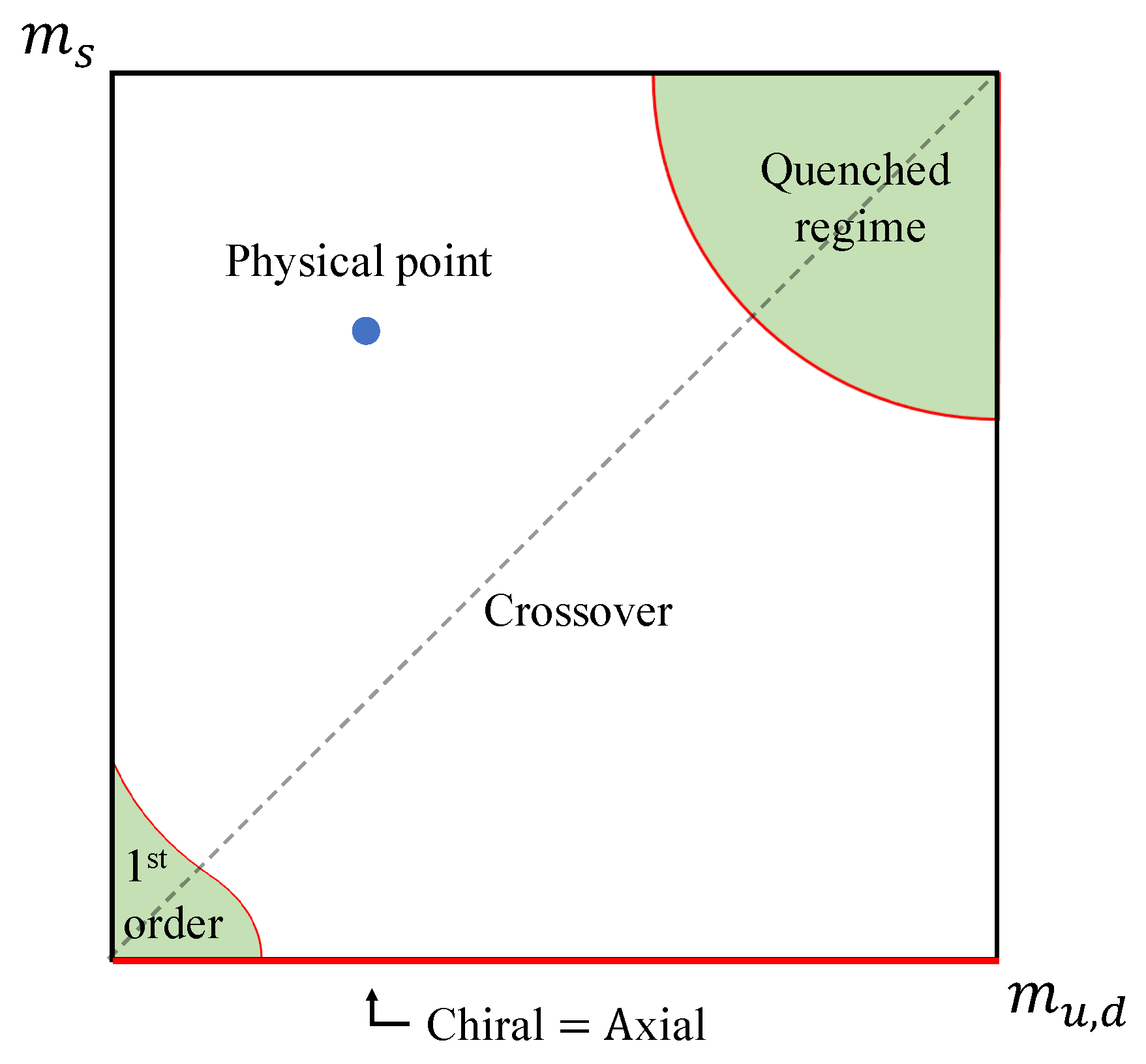
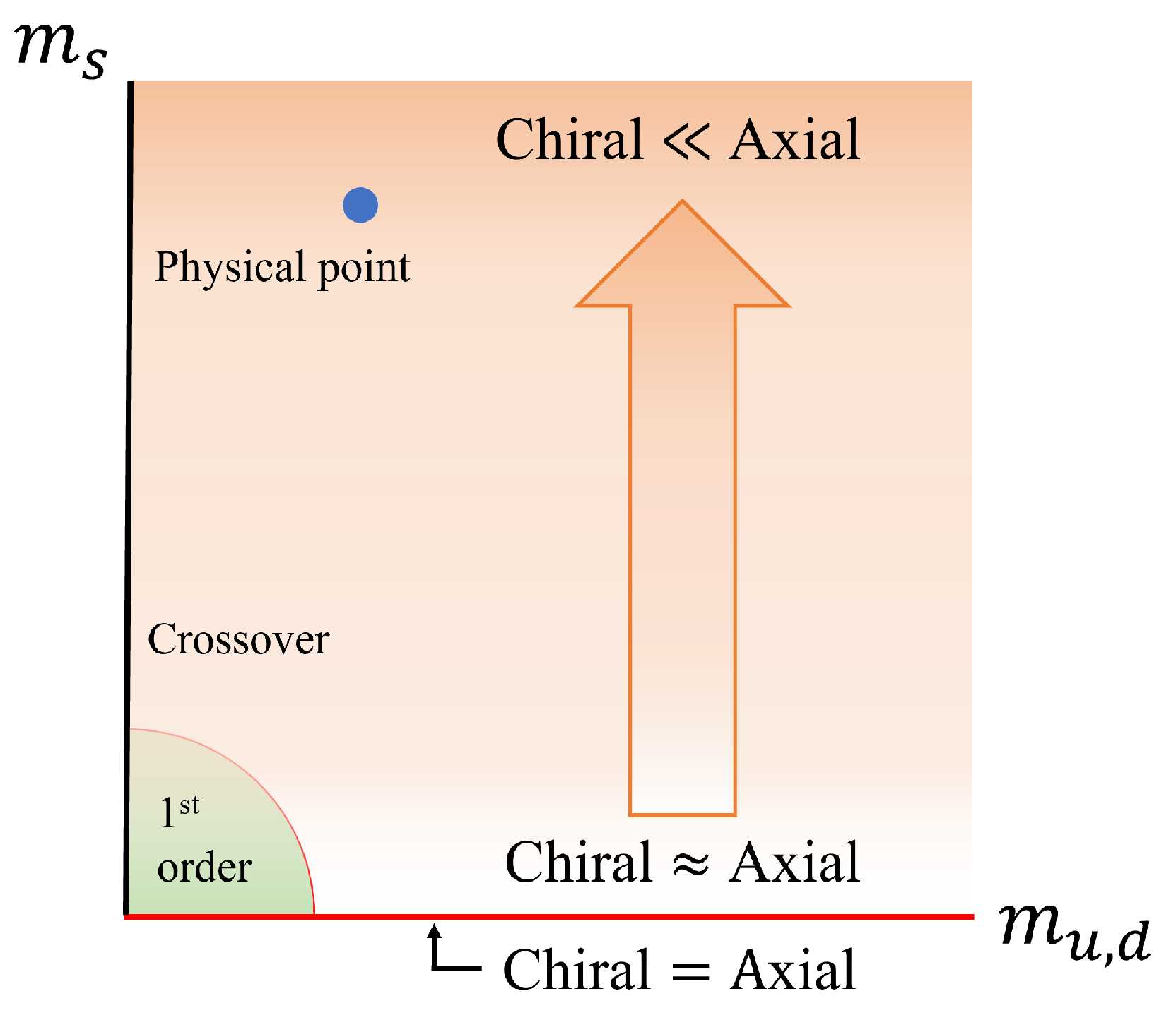
With those preliminaries, we may now pay attention to the Columbia plot to consider the quark mass dependence on the symmetry restoration. Figure 1 shows the conventional Columbia plot where the QCD phase diagram is described on the – plane. As a result of Equation (22), the chiral symmetry is simultaneously restored with the axial symmetry on the -axis.
In the next section, in order to explain the implication of the nontrivial coincidence in Equation (22) on the chiral–axial phase diagram, we investigate the interference of the topological susceptibility for the chiral and axial symmetry breaking based on the NJL model. This is visualized by drawing the chiral–axial phase diagram in the – plane, describing the trend of the chiral and axial symmetry restoration.
3. Chiral and Axial Symmetry Breaking in Low-Energy QCD Description
3.1. Nambu–Jona–Lasinio Model
To make the qualitative understanding of the nontrivial correlation among susceptibility functions in Equation (21) more explicit, we employ an NJL-model analysis based on the chiral symmetry and the symmetry of the underlying QCD possessions. As mentioned later, the NJL model predictions are shown to be in good agreement with the lattice QCD results at finite temperatures. In this subsection, we briefly introduce the NJL model description. Later, we show the formulae for the susceptibility functions in the framework of the NJL model approach.
The NJL model Lagrangian with three quark flavors is given as
The four-quark interaction term is invariant under the chiral transformation: , where with () being the Gell–Mann matrices in the flavor space together with and being the chiral phases. It takes the form
where is the coupling constant.
In the NJL model approach, the anomalous part is described by the determinant form, called the Kobayashi–Maskawa–‘t Hooft (KMT) term [26,27,28,29],
with the constant real parameter . Note that the axial breaking , which is induced from the QCD instanton configuration, still keeps the chiral symmetry.
The current conservation of the chiral symmetry and the symmetry becomes anomalous because of the presence of the quark mass terms and the KMT term:
where the terms within the curly brackets () represent an anticommutator. In the spirit of effective models based on the underlying QCD, the anomalous conservation laws of the NJL model have to be linked with those of the underlying QCD, as in Equation (8). Thus, the KMT operator, , may mimic the anomaly of the gluonic operator, . One should notice here that the anomaly described by the KMT term can vanish by taking . As far as the anomaly contribution is concerned, this limit corresponds to turning off the QCD gauge coupling g, which is equivalent to the trivial limit for the vanishing axial anomaly. (Note that even in the case of the vanishing anomaly associated with the NJL model is still an interacting theory because of the existence of the four-quark interaction term. Although is not completely compatible with the QCD coupling constant g, we can monitor the anomaly contribution through the effective coupling constant .)
3.2. Mean-Field Approximation and Vacuum of NJL Model
In this work, we employ the mean-field approximation corresponding to the large expansion. Within the mean-field approximation, the interaction terms are as follows:
where , and denote the quark condensates,
In the isospin symmetric limit (), and are taken as . Hence, the NJL Lagrangian is reduced to the mean-field Lagrangian :
where represents the mass matrix of the dynamical quarks,
By integrating out the quark field in the generating functional of the mean-field Lagrangian, the effective potential at finite temperature is evaluated as (see e.g., [30])
where denotes the number of colors and represents the energies of the constituent quarks. The NJL model is a nonrenormalizable theory. Hence, the momentum cutoff should be prescribed in the quark loop calculation to regularize the ultraviolet divergence. In Equation (31), we apply a sharp cutoff regularization to the three-dimensional momentum integration.
The quark condensates sit on the stationary point of the effective potential with respect to , , and , which are determined from the stationary conditions for the effective potential,
By solving the stationary conditions, one can obtain the following analytic expression of the quark condensates, which corresponds to the quark one-loop result:
3.3. Scalar- and Pseudoscalar-Meson Susceptibility in NJL Model
In this subsection, we introduce the pseudoscalar meson susceptibilities in the NJL model approach. First, the pseudoscalar susceptibilities, which construct the meson susceptibilities in Equation (2), are evaluated as [31]
with the external momentum . The susceptibilities are defined by the two-point correlation function of the quark bilinear field at the zero external momentum, .
We work in the random-phase approximation [31] so that the pseudoscalar susceptibilities are evaluated only through the resummed polarization diagram of the quark loop, taking into account the four-point interactions in the NJL model. Within the mean-field approximation, these four-point interaction terms represent fluctuations from the vacuum characterized by the nonzero quark condensates,
Here, we pick up only the interaction terms relevant to . Note that since we keep the isospin symmetry, i.e., , the four-point interaction terms proportional to vanish; hence, those terms do not come into play in the later discussion. Then, the pseudoscalar susceptibilities are expressed as
with
where is the coupling strength corresponding to the four-point interaction within the mean field approximation and is the polarization function at the quark one-loop level. Note that , , and take a matrix form.
The pion susceptibility corresponds to this with as
where the coupling strength in the pion channel and the pion polarization function are given as
with being the pesudoscalar one-loop polarization functions [32],
Note that owing to the isospin symmetry, and exhibit no off-diagonal components. In contrast, as shown in Equation (36), the flavor symmetry breaking associated with the anomaly provides off-diagonal components in and for ,
The pseudoscalar susceptibilities in Equation (5) are obtained as linear combinations of for as
where we take the isospin symmetric limit into account, i.e., and . Then, the meson susceptibility is evaluated as
Similarly, the scalar meson susceptibilities are given by
with
where is the coupling strength matrix and is the polarization tensor matrix in the scalar channel.
The explicit formula for reads
where the coupling strength in the meson channel and the -meson polarization function are given as
with being the scalar one-loop polarization functions,
For , and are given as
3.4. Trivial and Nontrivial Coincidence of Chiral and Axial Breaking in a View of the NJL Description
With Equation 20 and the pseudscalar meson susceptibility in Equations (38) and (44), the topological susceptibility in the NJL model can be described as
Using Equation (54) together with the meson susceptibilities in Equations (38), (44), (47) and (53), one can easily check that the NJL model reproduces Equation (21):
Note that the analytical expression of in Equation (54) explicitly shows that is proportional to the anomaly-related coupling . As is noted earlier, goes away in the limit of the vanishing anomaly, , while the meson susceptibility functions keep finite values. This is the NJL-model realization of the trivial coincidence between the indicators for the chiral and axial symmetry breaking in the meson susceptibility functions, as in Equation (9):
Of crucial is to note that in Equation (54) is also proportional to both the light quark mass and the strange quark mass, as the consequence of the flavor-singlet nature in Equation (19). Hence, the NJL model also provides the nontrivial coincidence between the chiral and axial indicators with keeping the anomaly, as derived from the underlying QCD in Equation (22):
This coincidence implies that the anomaly contribution in the associated meson channels becomes invisible in the meson susceptibility functions at where , even in the presence of the anomaly ().
The topological susceptibility has also been studied by some effective model approaches [33,34,35,36,37,38,39,40,41,42]. However, the previous studies did not consider the flavor-singlet nature of the topological susceptibility, so the nontrivial coincidence in Equation (56) has never been addressed. (one may further rotate quark fields by the transformation with the rotation angles , so that the NJL Lagrangian is shifted as , where and . By taking the , the -dependence is completely rotated away from the quark mass term and then moves to the term: . Indeed, the topological susceptibility has been evaluated based on the NJL Lagrangian including the term: [33]. However, the -dependence on the term accidentally goes away within the ordinary mean-field approach. This is because vanishes under the mean-field approximation, . Hence, the topological susceptibility cannot be evaluated based on within the mean-field approach through the second derivative of the generating functional with respect to . Therefore, we do not take this way; instead, we directly apply the Equation (18), which is evaluated from the -dependent quark-mass term with the flavor-singlet nature.)
4. Quark Mass Dependence on QCD Vacuum Structure
In this section, through Equation (21), we numerically explore the correlations among the susceptibility functions for the chiral symmetry breaking, the axial symmetry breaking, and the topological charge.
4.1. QCD Vacuum Structure with Physical Quark Masses
To exhibit the numerical results of the susceptibility functions, we take the value of the parameters as listed in Table 1 [31]. With the input values, the following four hadronic observables are obtained at [31]:
which are in good agreement with the experimental values. Furthermore, the topological susceptibility at the vacuum () qualitatively agrees with the lattice observations [43,44], as discussed in [23].
We do not consider intrinsic temperature-dependent couplings; instead, all the T dependence should be induced only from the thermal quark loop corrections. Actually, the present NJL shows good agreement with lattice QCD results on the temperature scaling for the chiral, axial, and topological susceptibilities, as shown in Ref. [23]. In this sense, we do not need to introduce such an intrinsic T dependence for the model parameters in the regime up to temperatures around the chiral crossover.
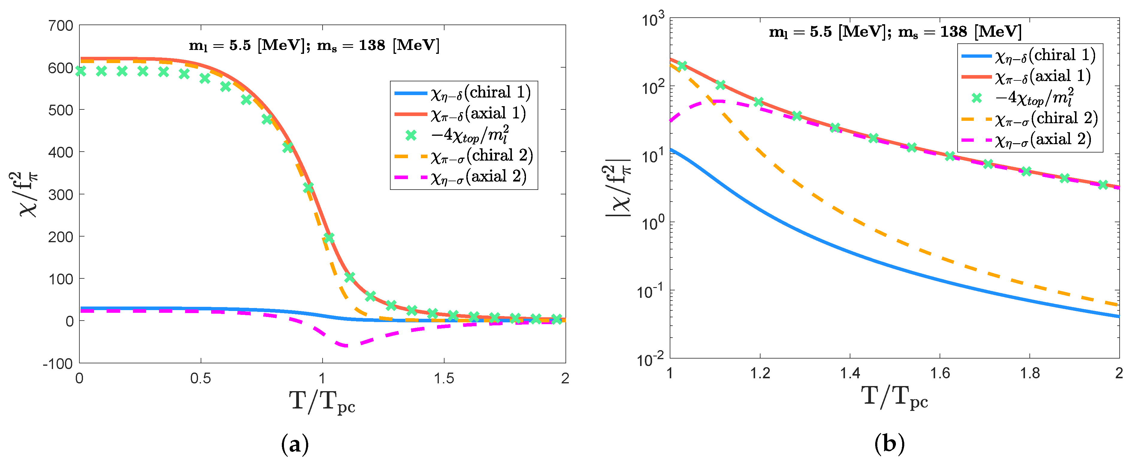
In Figure 2, we first show plots of the susceptibilities as a function of temperature. This figure shows that the meson susceptibilities forming the chiral partners (chiral indicators), and , approach zero smoothly at high temperatures but do not exactly reach zero. This tendency implies that the NJL model undergoes a chiral crossover. (What we work on are the susceptibilities, which correspond to meson-correlation functions at zero momentum transfer. This is in contrast to the conventional meson correlators depending on the transfer momentum, off which meson masses are read. Furthermore, the susceptibilities involve contact term contributions independent of momenta, which can be sensitive to high-energy scale physics, while the conventional meson correlators are dominated by the low-lying meson mass scale. Nevertheless, the degeneracy of the chiral or axial partners at high temperatures, similar to those detected in the susceptibility, can also be seen in the mass difference or equivalently the degeneracy of the conventional meson correlators for the partners, which is simply because the mass difference plays an alternative indicator of the chiral or axial breaking, as observed in the lattice simulation [45].)
The pseudocritical temperature of the chiral crossover can be evaluated from the inflection point of or with respect to temperature, , and then, we find MeV. This inflection point coincides with that estimated from the light quark condensate [23]. However, the NJL’s estimate of the pseudocritical temperature is somewhat bigger than the lattice QCD’s, MeV [10,46,47]. In fact, the NJL analysis is implemented in the mean-field approximation corresponding to the large limit. The corrections of the beyond mean-field approximation are subject to the size of the next-to-leading order corrections of the large expansion, . Including the possible corrections to the current model analysis, the NJL’s result may be consistent with the lattice observation. Supposing this systematic deviation by about to be accepted within the framework of the large expansion, one may say that the NJL description at finite temperatures yields qualitatively good agreement with the lattice QCD simulations. Indeed, all the temperature dependence of , , and qualitatively accords with the lattice data [9,10,43,44,48] (for a detailed discussion, see [23]).
From panel (a) of Figure 2, one can see a sizable difference in the meson susceptibilities between the chiral indicator and the axial indicator in the low temperature regime: for . A large discrepancy also shows up in the other combination between and : for . Looking at the high temperature regime , one finds that the sizable difference is still kept, , while and get close to zero, as shown in panel (b) of Figure 2. This tendency is actually consistent with the lattice QCD observation [9,10]. In addition, we find that becomes larger than at around . As the temperature increases further, and also approach zero with keeping for . These trends imply that the chiral symmetry is restored faster than the the symmetry in the meson susceptibility functions at the physical value of the current quark masses.
Hereafter, we vary the current quark masses while keeping the input values of the coupling constants , , and the cutoff and investigate the correlations among the susceptibility functions through Equation (21) as well as the nontrivial coincidence in Equation (22). Actually, in the present NJL model, as the current quark masses decrease, the chiral crossover is changed to the chiral second-order phase transition at MeV (corresponding to ). Thus, the chiral first-order phase-transition domain appears for < 60 MeV. In the subsequent subsections, we focus on the chiral crossover and the first-order phase-transition domainmains separately.
4.2. Crossover Domain
In this subsection, we evaluate the strange quark mass dependence on the susceptibility functions in the crossover domain. We allow the strange quark mass to be off the physical value, while the light quark mass is fixed at the physical one; MeV. The present NJL model with this setup exhibits the crossover for the chiral phase transition.
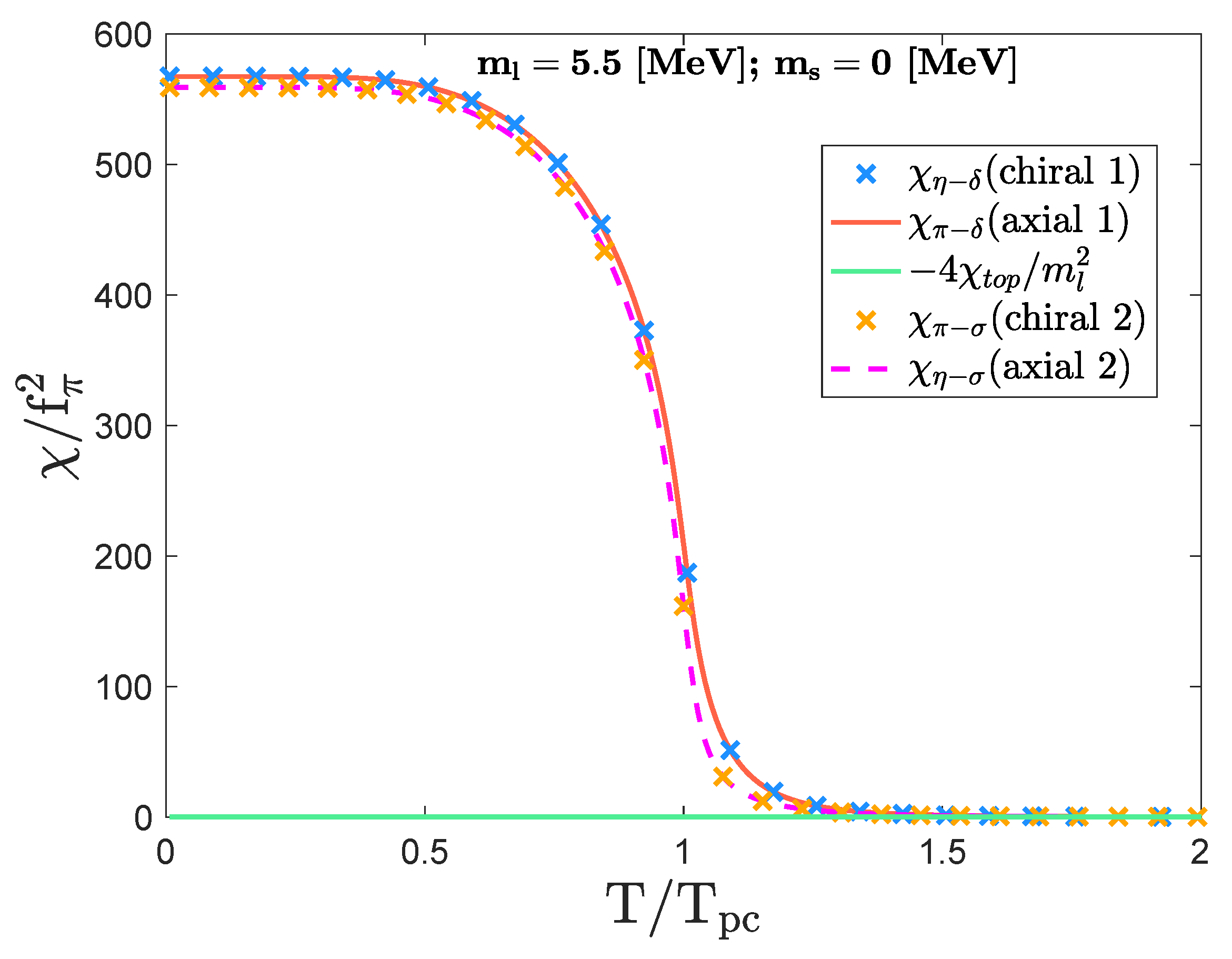
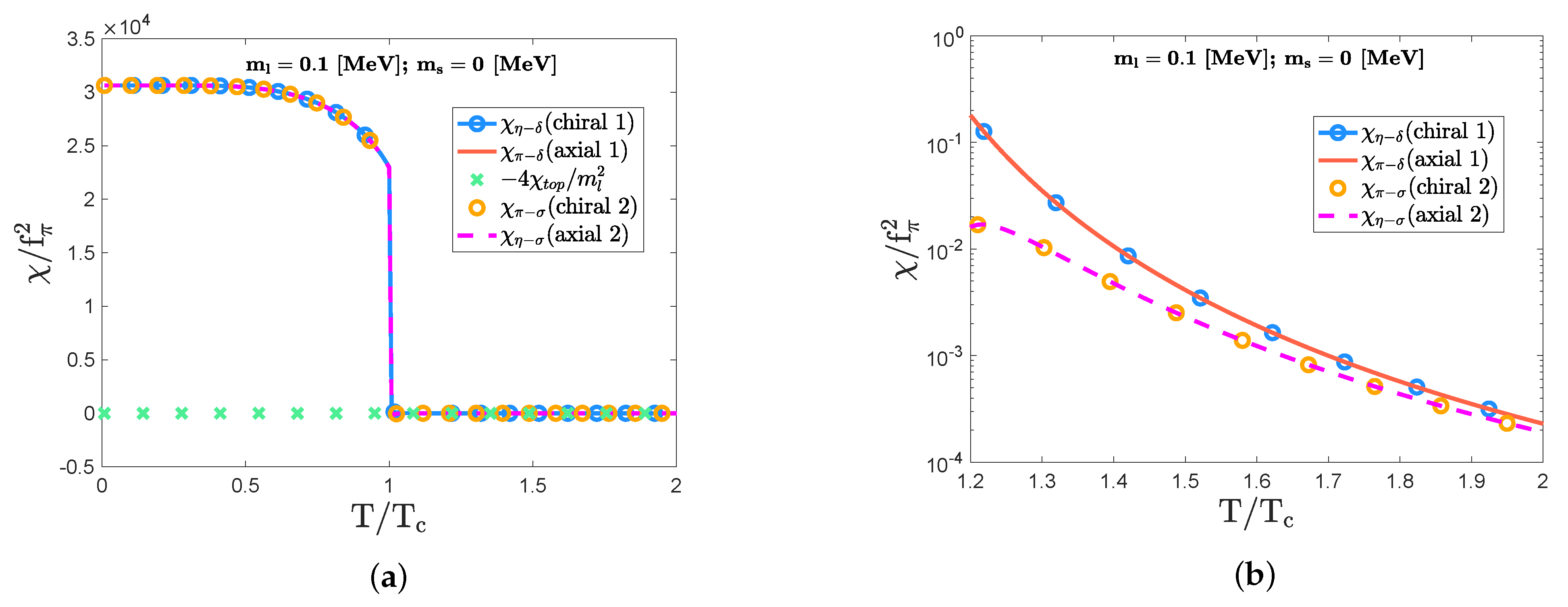
In Figure 3, we plot the susceptibility functions in the massless limit of the strange quark mass (). This figure shows that the topological susceptibility vanishes for any temperature. This must be due to the flavor-singlet nature in Equation (19). As a consequence of the vanishing , the axial indicator () coincides with the chiral indicator () for the whole temperature regime, so the chiral symmetry is simultaneously restored with the symmetry.
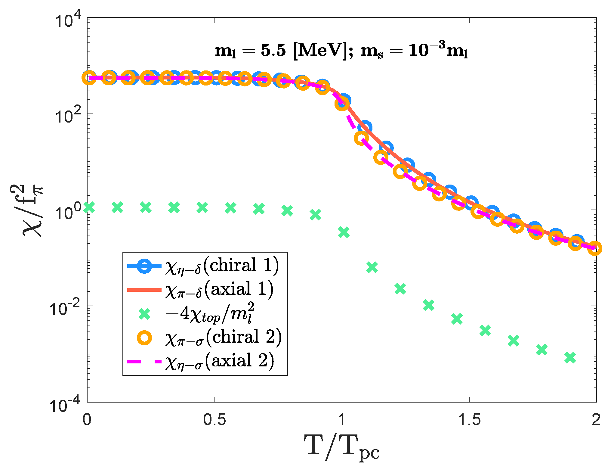
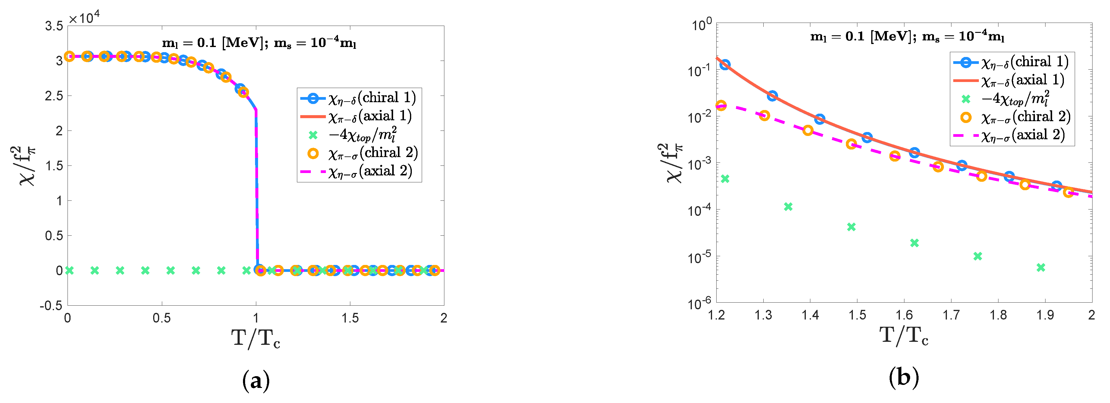
Once a finite strange quark mass is turned on, the topological susceptibility becomes finite no matter how small is, as seen in Figure 4. It is interesting to note that when , like in Figure 4 with , the topological susceptibility () is much smaller than the chiral indicator () and the axial indicator (). This is because is proportional to the , as the consequence of the flavor-singlet nature in Equation (19). According to the correlation among susceptibility functions in Equation (21), the chiral indicator () takes almost the same trajectory of what the axial indicator () follows at finite temperatures. Thus, it is the negligible that triggers the (almost) simultaneous symmetry restoration for the chiral and axial symmetries in the case of the tiny strange quark mass, where .
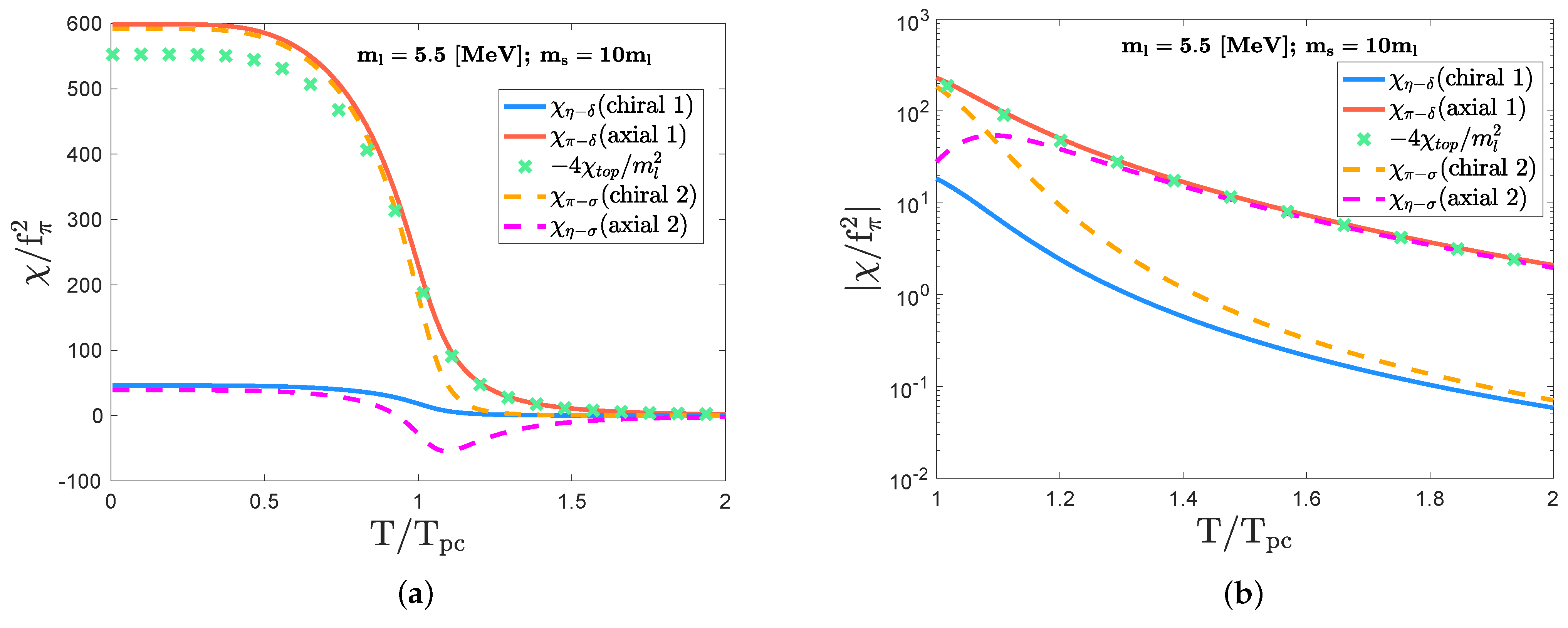
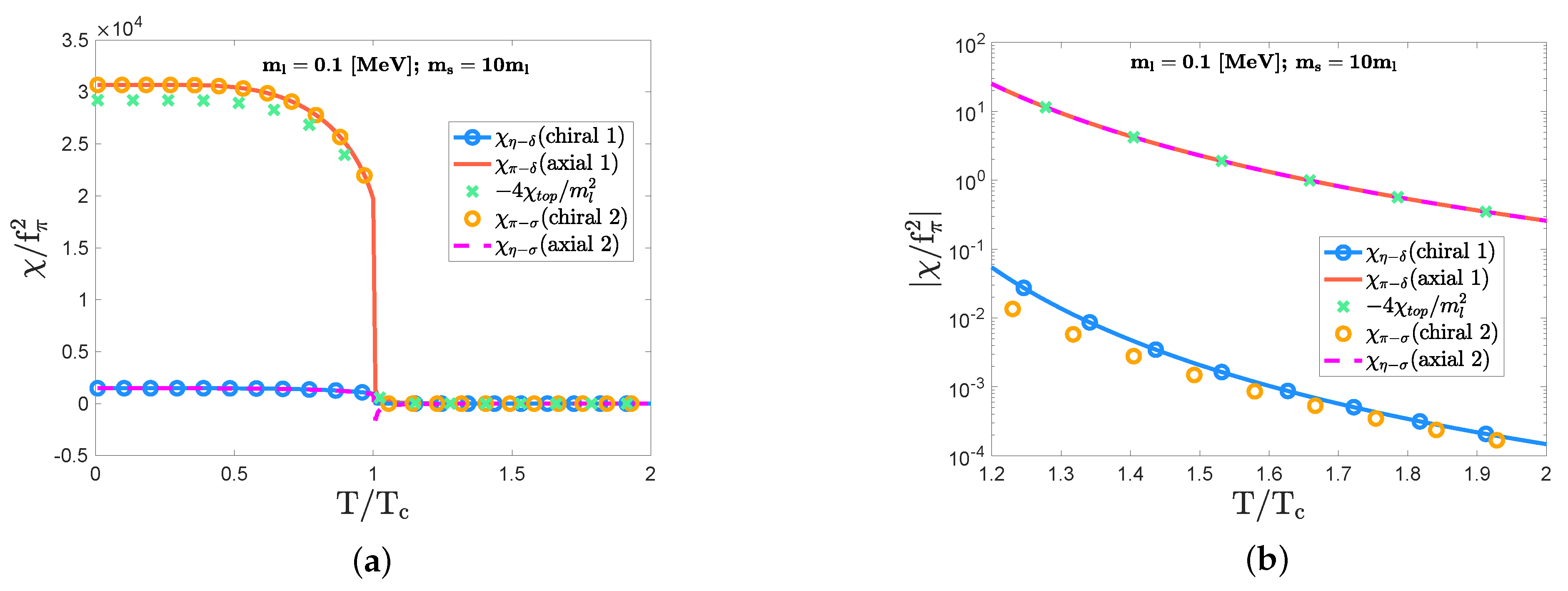
As increases, the topological susceptibility further grows, and starts to significantly contribute to the chiral and axial indicators following the correlation form in Equation (21). Actually, when the strange quark mass takes , the topological susceptibility () becomes on the same order of magnitude of and in the low temperature regime: for . This trend is depicted in panel (a) of Figure 5 for . Thus, the sizable discrepancy between the chiral indicator () and the axial indicator () for is due to the interference of . As the temperature further increases, the susceptibilities go to zero. However, a sizable discrepancy still appears between the chiral and axial indicators: and for , as depicted in panel (b) of Figure 5. This indicates that the large strange quark mass providing the significant interference of the topological susceptibility urges a faster restoration of the chiral symmetry for .
4.3. First-Order Domain
We next consider the first-order phase-transition domain. In this subsection, we fix the light quark mass as MeV and vary the strange quark mass . This setup leads to the first-order phase transition for the chiral symmetry.
First of all, see Figure 6, which shows the susceptibility functions for . One can find a jump in meson susceptibility functions at the critical temperature MeV. This jump indicates that the chiral first-order phase transition occurs in the NJL model. Note that, even for , the meson susceptibility functions take finite values because of the presence of the finite light-quark mass, as shown in panel (b) of Figure 6. This implies that the chiral and axial symmetries are not completely restored. However, the topological susceptibility is exactly zero because , reflecting the flavor-singlet nature of . This is why we observe and for the whole temperature (see Figure 6). In particular, panel (b) of Figure 6 shows that () asymptotically goes to zero along with () as the temperature increases. Thus, the chiral symmetry tends to simultaneously restore with the axial symmetry even in the chiral first-order phase-transition domain.
Next, we supply a finite value for the strange quark mass to see that the non-vanishing certainly emerges in the first-order phase-transition domain, as in the case of the chiral crossover domain. See Figure 7. As long as the strange quark mass is small enough, i.e., , the topological susceptibility is negligible compared with the chiral and axial indicators. Therefore, the coincidence between the chiral and axial symmetry restoration is effectively almost intact.
As the strange quark mass further increases, the topological susceptibility develops to be non-negligible. For , the topological susceptibility () significantly interferes with the chiral and axial indicators via Equation (21) and becomes comparable to and for (see Figure 8). For , we observe a large discrepancy— and — due to the significant contribution of the topological susceptibility. Thus, the sizable strange quark mass makes the chiral restoration faster than the axial restoration through the non-negligible contribution of the topological susceptibility. Indeed, these trends of the strange quark mass controlling in the first-order phase-transition domain are similar to those observed in the chiral crossover domain.
4.4. Chiral and Axial Symmetry Restorations in View of Chiral–Axial Phase Diagram
In the previous subsections, it is found that the topological susceptibility handled by the strange quark mass is closely related to the meson susceptibilities and interferes with the strengths of the chiral and axial symmetry breaking. Here, we clarify more on the strange quark mass dependence on the restoration trends of the chiral and axial symmetry.
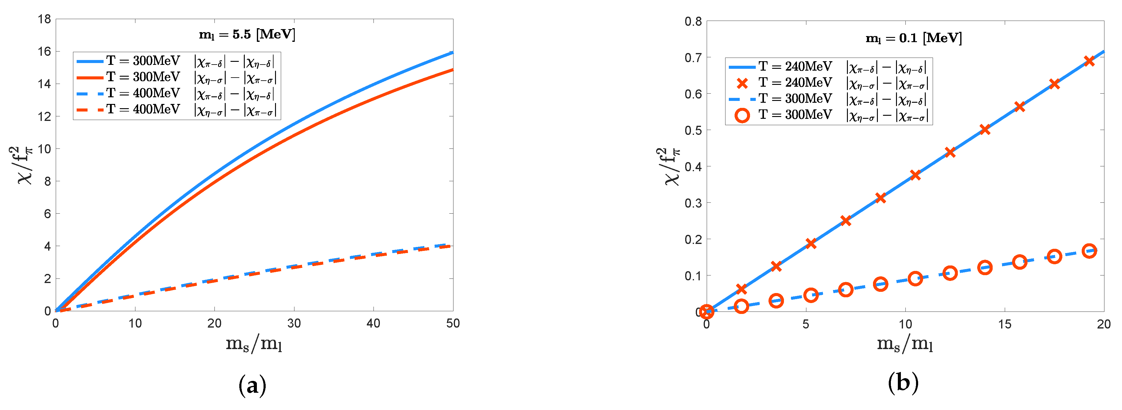
In Figure 9, we plot the strange quark mass dependence on the difference between the two indicators, and , above the (pseudo)critical temperature . In particular, and are realized at even after reaching a high temperature regime where . This implies that in the case of the massless strange quark, the simultaneous restoration for the chiral and axial symmetries takes place in both the chiral crossover and first-order phase-transition domains. Once the strange quark obtains a finite mass, the axial indicator () starts to deviate from the chiral indicator () because of the emergence of nonzero . Actually, Figure 9 shows that the strength of the axial symmetry breaking in the meson susceptibilities is enhanced by the finite strange quark mass through the interference of the topological susceptibility. Furthermore, the discrepancy between the axial indicator () and the chiral indicator () persists even at the high temperature . Therefore, the axial restoration tends to be delayed, occurring later than the chiral restoration as the strange quark mass gets heavier.
Finally, we draw the predicted tendency of the chiral and axial restorations in a chiral–axial phase diagram on the – plane, which is shown in Figure 10. This phase diagram is a sort of the Columbia plot, in which we reflect the discrepancy between the chiral and axial restorations in terms of the meson susceptibilities at around .
5. Summary and Discussion
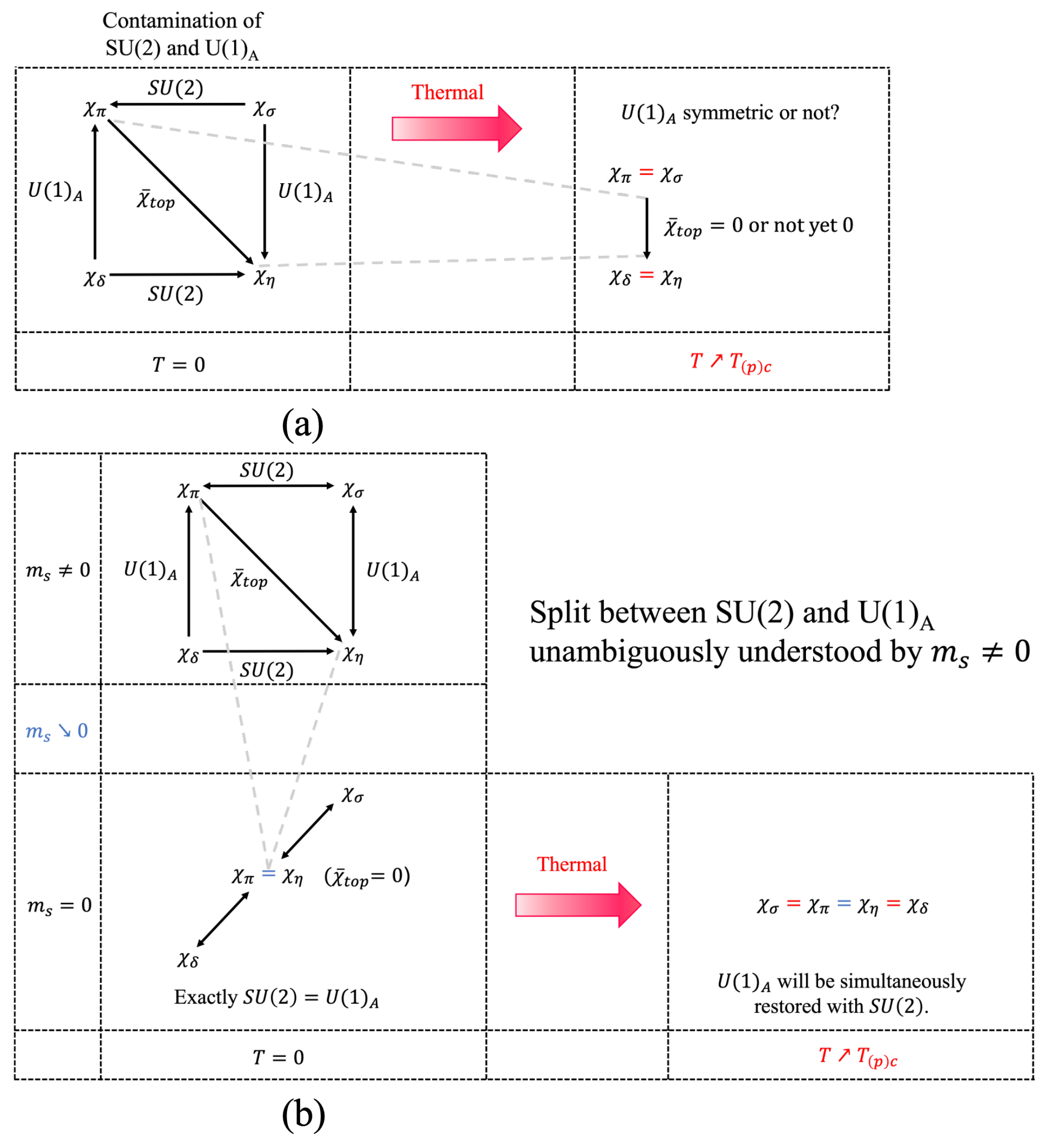
The anomalous chiral-Ward identity in Equation (20) relating the topological susceptibility to the pseudoscalar meson susceptibility functions has often been used to measure the effective restoration of the axial symmetry in the chiral symmetric phase so far. The restoration probed by the topological susceptibility has been studied extensively in the chiral effective model approaches [33,34,35,36,37,38,39,40,41,42] and the lattice QCD frameworks [9,10,43,44,48] to explore the origin of the split in restorations of the chiral symmetry and the axial symmetry. This ordinary method is summarized in panel (a) of Figure 11). However, this ordinary approach suffers from practical difficulty in accessing the origin of the split without ambiguity because the chiral symmetry breaking is highly contaminated with the axial symmetry breaking even at the beginning, at the vacuum.
In this paper, we find a new approach: it is the strange quark mass that controls the strengths of the chiral symmetry breaking and the axial symmetry breaking, and those strengths coincide in the limit . The idea is to depart from a nontrivial coincidence limit emerging even in the presence of nonzero anomaly due to the nonperturbatively interacting QCD, in sharp contrast to the trivial equivalence between the chiral and axial breaking, where QCD gets reduced to the free quark theory. Of course, the nontrivial coincidence is robust because it is tied with the anomalous chiral Ward–Takahashi identity, Equation (21), and the flavor-singlet condition of the topological susceptibility. Hence, it holds even at finite temperatures, so the chiral symmetry is simultaneously restored with the axial symmetry regardless of the order of the chiral phase transition.
The simultaneous restoration at is viewed as a significant limit to consider the symmetry restorations on the quark mass plane. Given the “rigid” limit of , we can unambiguously understand that the split in the restorations of the chiral and is handled by the strange quark mass (). This new point of view for symmetry restorations is described in panel (b) of Figure 11.
To be concrete, we employ the NJL model with three flavors to monitor the essential chiral and axial features that QCD possesses. We confirm that the NJL model surely provides the nontrivial coincidence of the chiral and axial breaking in the case of in terms of the meson susceptibility functions and exhibits the simultaneous restoration for the chiral and axial symmetries in both the chiral crossover and the first-order phase-transition cases:
Once the strange quark gets massive, the topological susceptibility takes a finite value and interferes with the meson susceptibility functions through Equation (21). The simultaneous restoration for the chiral and axial symmetries is controlled by the strange quark mass through the interference of nonzero . Thus, with the large strange quark mass (), the chiral restoration significantly deviates from the axial restoration above the (pseudo)critical temperature:
Because of the significant interference of the topological susceptibility, the chiral symmetry is restored faster than the axial symmetry in the flavor case with the physical quark masses. Figure 10 shows a schematic view of the evolution of the chiral and axial breaking deviating from the nontrivial coincidence limit toward real-life QCD.
In closing the present paper, we give a list of several comments on our findings and another intriguing aspect of the nontrivial coincidence between the chiral and axial symmetry breaking strengths.
- The predicted chiral–axial phase diagram in Figure 10 is a new guideline for exploring the influence of the anomaly on the chiral phase transition, which is sort of giving a new interpretation of the conventional Columbia plot. Further studies are desired in lattice QCD simulations to draw definitely conclusive benchmarks on the chiral–axial phase diagram.
- The existence of the nontrivial coincidence implies that the anomaly can be controlled by the current mass of the strange quark. The controllable anomaly can give a new understanding of the meson mass originated from the anomaly. The investigation for the -dependence on the pseudoscalar meson masses will thus be a valuable study.
- The fate of the anomaly in the nuclear/quark matter is a longstanding problem and has attracted a lot of people so far. The nontrivial coincidence should also be realized in the finite dense matter involving the massless strange quark. The nontrivial coincidence at finite density may shed light on a novel insight for the partial restoration in the medium with physical quark masses.
- The contribution of the anomaly to the color confinement is an open question. It is worth including the Polyakov loop terms in the NJL model to address the correlation between the nontrivial coincidence of the chiral and axial breaking and the deconfinement–confinement phase transition.
- Though the NJL model produces the qualitative results consistent with lattice observations, it is a rough analysis due to the mean-field approximation. However, the existence of the nontrivial coincidence is robust because it is based on the anomalous Ward identity, This should thus be seen even beyond the mean-field approximation that the present NJL study has assumed or even more rigorous nonperturbative analyses, such as those based on the lattice NJL-model and the functional renormalization group method.
- The nontrivial chiral–axial coincidence is a generic phenomenon, which can also be seen in a generic class of QCD-like theories with “1 () + 2 () flavors”, involving models beyond the standard model. In particular, the coincidence in the first-order phase-transition case may impact cosmological implications of QCD-like scenarios with axionlike particles associated with the axial breaking, including the gravitational wave probes. Investigation along also this line may be interesting.
Author Contributions
Conceptualization, M.K.; Formal analysis, M.K.; Investigation, C.-X.C., J.-Y.L. and A.T.; Writing—original draft, M.K.; Writing—review and editing, S.M. All authors have read and agreed to the published version of the manuscript.
Funding
This work was supported in part by the National Science Foundation of China (NSFC) under Grant Nos. 11975108, 12047569, 12147217 and the Seeds Funding of Jilin University (S.M.). The work of A.T. was supported by the RIKEN Special Postdoctoral Researcher program and partially by JSPS KAKENHI Grant Numbers JP20K14479, 20K14479, 22H05112, and 22H05111. M.K. was supported by the Fundamental Research Funds for the Central Universities and partially by the National Natural Science Foundation of China (NSFC) Grant No: 12235016, and the Strategic Priority Research Program of Chinese Academy of Sciences under Grant No. XDB34030000. This work was also supported by MEXT as “Program for Promoting Researches on the Supercomputer Fugaku” (Grant Number JPMXP1020230411) and “Program for Promoting Researches on the Supercomputer Fugaku” (Search for physics beyond the standard model using large-scale lattice QCD simulation and development of AI technology toward next-generation lattice QCD; Grant Number JPMXP1020230409).
Data Availability Statement
No new data were created or anlyzed in this study. Date sharing is not applicable to this article.
Acknowledgments
We are grateful to Hen-Tong Ding for useful comments.
Conflicts of Interest
The authors declare no conflicts of interest.
References
- Pisarski, R.D.; Wilczek, F. Remarks on the Chiral Phase Transition in Chromodynamics. Phys. Rev. D 1984, 29, 338–341. [Google Scholar] [CrossRef]
- Ejiri, S.; Karsch, F.; Laermann, E.; Miao, C.; Mukherjee, S.; Petreczky, P.; Schmidt, C.; Soeldner, W.; Unger, W. On the magnetic equation of state in (2+1)-flavor QCD. Phys. Rev. D 2009, 80, 094505. [Google Scholar] [CrossRef]
- Kaczmarek, O.; Karsch, F.; Laermann, E.; Miao, C.; Mukherjee, S.; Petreczky, P.; Schmidt, C.; Soeldner, W.; Unger, W. Phase boundary for the chiral transition in (2+1) -flavor QCD at small values of the chemical potential. Phys. Rev. D 2011, 83, 014504. [Google Scholar] [CrossRef]
- Engels, J.; Karsch, F. The scaling functions of the free energy density and its derivatives for the 3d O(4) model. Phys. Rev. D 2012, 85, 094506. [Google Scholar] [CrossRef]
- Burger, F.; Ilgenfritz, E.M.; Kirchner, M.; Lombardo, M.P.; Müller-Preussker, M.; Philipsen, O.; Urbach, C.; Zeidlewicz, L. Thermal QCD transition with two flavors of twisted mass fermions. Phys. Rev. D 2013, 87, 074508. [Google Scholar] [CrossRef]
- Bazavov, A.; Ding, H.T.; Hegde, P.; Kaczmarek, O.; Karsch, F.; Karhtik, N.; Laermann, E.; Lahiri, A.; Larsen, R.; Li, S.T.; et al. Chiral crossover in QCD at zero and non-zero chemical potentials. Phys. Lett. B 2019, 795, 15–21. [Google Scholar] [CrossRef]
- Ding, H.T.; Hegde, P.; Kaczmarek, O.; Karsch, F.; Lahiri, A.; Larsen, R.; Mukherjee, H.; Ohno, P.; Schmidt, C.; Steinbrecher, P.; et al. Chiral Phase Transition Temperature in (2+1)-Flavor QCD. Phys. Rev. Lett. 2019, 123, 062002. [Google Scholar] [CrossRef]
- Brown, F.R.; Butler, F.P.; Chen, H.; Christ, N.H.; Dong, Z.h.; Schaffer, W.; Unger, L.I.; Vaccarino, A. On the existence of a phase transition for QCD with three light quarks. Phys. Rev. Lett. 1990, 65, 2491–2494. [Google Scholar] [CrossRef]
- Buchoff, M.I.; Cheng, M.; Christ, N.H.; Ding, H.-T.; Jung, C.; Karash, F.; Lin, Z.; Mawhinney, R.D.; Mukherjee, S.; Petreczky, P.; et al. QCD chiral transition, U(1)A symmetry and the dirac spectrum using domain wall fermions. Phys. Rev. D 2014, 89, 054514. [Google Scholar] [CrossRef]
- Bhattacharya, T.; Buchoff, M.I.; Christ, N.H.; Ding, H.-T.; Gupta, R.; Karsch, C.J.F.; Lin, Z.; Mawhinney, R.D.; McGlynn, G.; Mukherjee, S.; et al. QCD Phase Transition with Chiral Quarks and Physical Quark Masses. Phys. Rev. Lett. 2014, 113, 082001. [Google Scholar] [CrossRef]
- Ding, H.T.; Li, S.T.; Mukherjee, S.; Tomiya, A.; Wang, X.D.; Zhang, Y. Correlated Dirac Eigenvalues and Axial Anomaly in Chiral Symmetric QCD. Phys. Rev. Lett. 2021, 126, 082001. [Google Scholar] [CrossRef]
- Cohen, T.D. The High temperature phase of QCD and U(1)-A symmetry. Phys. Rev. D 1996, 54, R1867–R1870. [Google Scholar] [CrossRef] [PubMed]
- Aoki, S.; Fukaya, H.; Taniguchi, Y. Chiral symmetry restoration, eigenvalue density of Dirac operator and axial U(1) anomaly at finite temperature. Phys. Rev. D 2012, 86, 114512. [Google Scholar] [CrossRef]
- Cossu, G.; Aoki, S.; Fukaya, H.; Hashimoto, S.; Kaneko, T.; Matsufuru, H.; Noaki, J.I. Finite temperature study of the axial U(1) symmetry on the lattice with overlap fermion formulation. Phys. Rev. D 2013, 87, 114514, Erratum in Phys. Rev. D 2013, 88, 019901. [Google Scholar] [CrossRef]
- Tomiya, A.; Cossu, G.; Aoki, S.; Fukaya, H.; Hashimoto, S.; Kaneko, T.; Noaki, J. Evidence of effective axial U(1) symmetry restoration at high temperature QCD. Phys. Rev. D 2017, 96, 034509, Erratum in Phys. Rev. D 2017, 96, 079902. [Google Scholar] [CrossRef]
- Aoki, S.; Aoki, Y.; Cossu, G.; Fukaya, H.; Hashimoto, S.; Kaneko, T.; Rohrhofer, C.; Suzuki, K. Study of the axial U(1) anomaly at high temperature with lattice chiral fermions. Phys. Rev. D 2021, 103, 074506. [Google Scholar] [CrossRef]
- Baluni, V. CP Violating Effects in QCD. Phys. Rev. D 1979, 19, 2227–2230. [Google Scholar] [CrossRef]
- Kim, J.E. Light Pseudoscalars, Particle Physics and Cosmology. Phys. Rept. 1987, 150, 1–177. [Google Scholar] [CrossRef]
- Kawaguchi, M.; Matsuzaki, S.; Tomiya, A. Analysis of nonperturbative flavor violation at chiral crossover criticality in QCD. Phys. Rev. D 2021, 103, 054034. [Google Scholar] [CrossRef]
- Gómez Nicola, A.; Ruiz de Elvira, J. Pseudoscalar susceptibilities and quark condensates: Chiral restoration and lattice screening masses. J. High Energy Phys. 2016, 03, 186. [Google Scholar] [CrossRef]
- Gomez Nicola, A.; Ruiz de Elvira, J. Patterns and partners for chiral symmetry restoration. Phys. Rev. D 2018, 97, 074016. [Google Scholar] [CrossRef]
- Gómez Nicola, A.; Ruiz De Elvira, J. Chiral and U(1)A restoration for the scalar and pseudoscalar meson nonets. Phys. Rev. D 2018, 98, 014020. [Google Scholar] [CrossRef]
- Cui, C.X.; Li, J.Y.; Matsuzaki, S.; Kawaguchi, M.; Tomiya, A. QCD Trilemma. arXiv 2021, arXiv:2106.05674. [Google Scholar]
- Witten, E. Current Algebra Theorems for the U(1) Goldstone Boson. Nucl. Phys. B 1979, 156, 269–283. [Google Scholar] [CrossRef]
- Veneziano, G. U(1) Without Instantons. Nucl. Phys. B 1979, 159, 213–224. [Google Scholar] [CrossRef]
- Kobayashi, M.; Maskawa, T. Chiral symmetry and eta-x mixing. Prog. Theor. Phys. 1970, 44, 1422–1424. [Google Scholar] [CrossRef]
- Kobayashi, M.; Kondo, H.; Maskawa, T. Symmetry breaking of the chiral u(3) x u(3) and the quark model. Prog. Theor. Phys. 1971, 45, 1955–1959. [Google Scholar] [CrossRef]
- ’t Hooft, G. Symmetry Breaking Through Bell-Jackiw Anomalies. Phys. Rev. Lett. 1976, 37, 8–11. [Google Scholar] [CrossRef]
- ’t Hooft, G. Computation of the Quantum Effects Due to a Four-Dimensional Pseudoparticle. Phys. Rev. D 1976, 14, 3432–3450, Erratum: Phys. Rev. D 1978, 18, 2199. [Google Scholar] [CrossRef]
- Klevansky, S.P. The Nambu-Jona-Lasinio model of quantum chromodynamics. Rev. Mod. Phys. 1992, 64, 649–708. [Google Scholar] [CrossRef]
- Hatsuda, T.; Kunihiro, T. QCD phenomenology based on a chiral effective Lagrangian. Phys. Rept. 1994, 247, 221–367. [Google Scholar] [CrossRef]
- Kunihiro, T. Chiral restoration, flavor symmetry and the axial anomaly at finite temperature in an effective theory. Nucl. Phys. B 1991, 351, 593–622. [Google Scholar] [CrossRef]
- Fukushima, K.; Ohnishi, K.; Ohta, K. Topological susceptibility at zero and finite temperature in the Nambu-Jona-Lasinio model. Phys. Rev. C 2001, 63, 045203. [Google Scholar] [CrossRef]
- Jiang, Y.; Zhuang, P. Functional Renormalization for Chiral and UA(1) Symmetries at Finite Temperature. Phys. Rev. D 2012, 86, 105016. [Google Scholar] [CrossRef]
- Jiang, Y.; Xia, T.; Zhuang, P. Topological Susceptibility in Three-Flavor Quark Meson Model at Finite Temperature. Phys. Rev. D 2016, 93, 074006. [Google Scholar] [CrossRef]
- Lu, Z.Y.; Ruggieri, M. Effect of the chiral phase transition on axion mass and self-coupling. Phys. Rev. D 2019, 100, 014013. [Google Scholar] [CrossRef]
- Gómez Nicola, A.; Ruiz De Elvira, J.; Vioque-Rodríguez, A. The QCD topological charge and its thermal dependence: The role of the η′. J. High Energy Phys. 2019, 11, 086. [Google Scholar] [CrossRef]
- Di Vecchia, P.; Veneziano, G. Chiral Dynamics in the Large n Limit. Nucl. Phys. B 1980, 171, 253–272. [Google Scholar] [CrossRef]
- Hansen, F.C.; Leutwyler, H. Charge correlations and topological susceptibility in QCD. Nucl. Phys. B 1991, 350, 201–227. [Google Scholar] [CrossRef]
- Leutwyler, H.; Smilga, A.V. Spectrum of Dirac operator and role of winding number in QCD. Phys. Rev. D 1992, 46, 5607–5632. [Google Scholar] [CrossRef]
- Bernard, V.; Descotes-Genon, S.; Toucas, G. Determining the chiral condensate from the distribution of the winding number beyond topological susceptibility. J. High Energy Phys. 2012, 12, 80. [Google Scholar] [CrossRef]
- Guo, F.K.; Meißner, U.G. Cumulants of the QCD topological charge distribution. Phys. Lett. B 2015, 749, 278–282. [Google Scholar] [CrossRef]
- Borsanyi, S.; Fodor, Z.; Guenther, J.; Hampert, K.-H.; Katz, S.D.; Kawanai, T.; Kovacs, T.G.; Mages, S.W.; Pasztor, A.; Pittler, F.; et al. Calculation of the axion mass based on high-temperature lattice quantum chromodynamics. Nature 2016, 539, 69–71. [Google Scholar] [CrossRef]
- Bonati, C.; D’Elia, M.; Martinelli, G.; Negro, F.; Sanfilippo, F.; Todaro, A. Topology in full QCD at high temperature: A multicanonical approach. J. High Energy Phys. 2018, 11, 170. [Google Scholar] [CrossRef]
- Brandt, B.B.; Francis, A.; Meyer, H.B.; Philipsen, O.; Robaina, D.; Wittig, H. On the strength of the UA(1) anomaly at the chiral phase transition in Nf=2 QCD. J. High Energy Phys. 2016, 12, 158. [Google Scholar] [CrossRef]
- Aoki, Y.; Borsanyi, S.; Durr, S.; Fodor, Z.; Katz, S.D.; Krieg, S.; Szabo, K.K. The QCD transition temperature: Results with physical masses in the continuum limit II. J. High Energy Phys. 2009, 6, 88. [Google Scholar] [CrossRef]
- Ding, H.T.; Karsch, F.; Mukherjee, S. Thermodynamics of strong-interaction matter from Lattice QCD. Int. J. Mod. Phys. E 2015, 24, 1530007. [Google Scholar] [CrossRef]
- Petreczky, P.; Schadler, H.P.; Sharma, S. The topological susceptibility in finite temperature QCD and axion cosmology. Phys. Lett. B 2016, 762, 498–505. [Google Scholar] [CrossRef]
Figure 1.
Conventional Columbia plot. The strength of chiral symmetry breaking coincides with the axial symmetry breaking strength in the meson susceptibility functions with because of the vanishing topological susceptibility. Thus, the simultaneous symmetry restoration between the chiral and is realized on the axis independently of the order of the chiral phase transition.

Figure 2.
The temperature dependence of the susceptibility functions at the physical point ( MeV and MeV) for (a) and (b) . The pseusocritical temperature for the chiral crossover is observed to be MeV. The susceptibility functions are normalized by square of the pion decay constant ( MeV), and the temperature axis is also normalized by , so all quantities are dimensionless to reduce the systematic uncertainty (approximately about 30%) associated with the present NJL model description of QCD. See also the text.

Figure 3.
The plot showing the nontrivial coincidence between the chiral and axial indicators (of two types) in the crossover domain with the massless strange quark ( MeV and ; MeV). The topological susceptibility is exactly zero for all temperatures because the flavor-singlet nature associated with the massless strange quark. Scaling factors are applied on both horizontal and vertical axes in the same way as in Figure 2.

Figure 4.
The plot showing the finiteness of the topological susceptibility along with the temperature dependence of the chiral and axial indicators in the crossover domain with a small strange quark mass ( MeV and ; MeV). The same scaling for two axes has been made as in Figure 2.
Figure 4.
The plot showing the finiteness of the topological susceptibility along with the temperature dependence of the chiral and axial indicators in the crossover domain with a small strange quark mass ( MeV and ; MeV). The same scaling for two axes has been made as in Figure 2.

Figure 5.
The plots clarifying the significant interference of the topological susceptibility to make the sizable discrepancy between the chiral and axial indicators in the crossover domain with the large strange quark mass ( MeV and = 10 ; MeV) for (a) and (b) . The manner of scaling axes is the same as in Figure 2.

Figure 6.
The plots clarifying the trend of the nontrivial simultaneous restoration for the chiral and axial symmetries even in the chiral first-order phase-transition domain with MeV and . Panel (a) shows a jump in the mesons susceptibility functions at around MeV as a consequence of the first-order phase transition. The panel (b) closes up the temperature dependence for the chiral and axial indicators after the chiral phase transition. The manner of scaling axes is the same as in Figure 2. The trend induced by the interference of is similar to the one observed in the crossover domain in Figure 3.

Figure 7.
The plots showing the still almost coincidence of the chiral and axial indicators for all temperature ranges, even in the first-order phase-transition domain with MeV and ; MeV. The two displayed axes are scaled in the same way as explained in the caption of Figure 2. The trend induced by the interference of is similar to the one observed in the crossover domain in Figure 4.

Figure 8.
The plots clarifying the significant interference of with the chiral and axial indicators in the first-order phase-transition domain with MeV and = 10 ; MeV. The two displayed axes are scaled in the same way as explained in the caption of Figure 2. The trend induced by the interference of is similar to the one observed in the crossover domain in Figure 5.

Figure 9.
The strange quark mass dependence on the difference between the axial indicator () and the chiral indicator () in (a) the crossover domain and (b) the first-order phase-transition domain. In the crossover domain with , the pseudocritical temperature is evaluated as MeV, and the temperatures MeV displayed as in panel (a) correspond to . On the other hand, in the first-order phase-transition domain, the temperatures MeV as fixed in panel (b) correspond to , where MeV for .

Figure 10.
The predicted chiral–axial phase diagram on the - plane, in which the discrepancy of the chiral and axial symmetry restorations at around is drawn by the shaded area. When the strength of the axial symmetry breaking deviates from the chiral breaking strength to be large, the shaded areas become thick. The nontrivial coincidence, as in Equation (22), is associated with the vanishing , which is located on the axis. When the strange quark mass obtains a finite mass, the axial restoration deviates from the chiral restoration. At around , the axial restoration is much later than the chiral restoration because of the significant interference of . Namely, at the physical quark masses, the topological susceptibility provides the large discrepancy between the chiral and axial restorations in the meson susceptibilities.

Figure 11.
The split in the restorations of the chiral symmetry and the axial symmetry at hot QCD. (a): Ordinary way to address the symmetry restorations. The ambiguous origin of the effective restoration is often measured by the topological susceptibility (which is normalized by the quark mass, ). (b): New point of view for symmetry restorations at . Because of the anomalous Ward–Takahashi identity at hot QCD, the chiral symmetry breaking exactly coincides with the symmetry breaking, and this coincidence holds for any temperatures. As a robust consequence, when the chiral symmetry is restored at the (pseudo)critical temperature, the symmetry is simultaneously restored. Therefore, the limit manifests the symmetry restorations on the quark mass plane: it can be unambiguously understood that the strange quark mass handles the split in the restorations of chiral symmetry and the symmetry at hot QCD with the three quark flavors having finite masses.


Table 1.
Parameter setting.
| Parameters | Values |
|---|---|
| light quark mass | 5.5 MeV |
| strange quark mass | 138 MeV |
| four-fermion coupling constant | 0.358 |
| six-fermion coupling constant | −0.0275 |
| cutoff | 631.4 MeV |
Disclaimer/Publisher’s Note: The statements, opinions and data contained in all publications are solely those of the individual author(s) and contributor(s) and not of MDPI and/or the editor(s). MDPI and/or the editor(s) disclaim responsibility for any injury to people or property resulting from any ideas, methods, instructions or products referred to in the content. |
© 2024 by the authors. Licensee MDPI, Basel, Switzerland. This article is an open access article distributed under the terms and conditions of the Creative Commons Attribution (CC BY) license (https://creativecommons.org/licenses/by/4.0/).
Share and Cite
MDPI and ACS Style
Cui, C.-X.; Li, J.-Y.; Matsuzaki, S.; Kawaguchi, M.; Tomiya, A. New Aspect of Chiral SU(2) and U(1) Axial Breaking in QCD. Particles 2024, 7, 237-263. https://0-doi-org.brum.beds.ac.uk/10.3390/particles7010014
AMA Style
Cui C-X, Li J-Y, Matsuzaki S, Kawaguchi M, Tomiya A. New Aspect of Chiral SU(2) and U(1) Axial Breaking in QCD. Particles. 2024; 7(1):237-263. https://0-doi-org.brum.beds.ac.uk/10.3390/particles7010014
Chicago/Turabian StyleCui, Chuan-Xin, Jin-Yang Li, Shinya Matsuzaki, Mamiya Kawaguchi, and Akio Tomiya. 2024. "New Aspect of Chiral SU(2) and U(1) Axial Breaking in QCD" Particles 7, no. 1: 237-263. https://0-doi-org.brum.beds.ac.uk/10.3390/particles7010014