Article

Teasing Apart Silvopasture System Components Using Machine Learning for Optimization

1
USDA-ARS, Crop Production System Research, Stoneville, MS 38776, USA
2
USDA-ARS, Poultry Production and Product Safety Research Unit, Fayetteville, AR 72701, USA
3
USDA-ARS, Dale Bumpers Small Farms Research Center, Booneville, AR 72927, USA
4
Animal Sciences Department, University of Arkansas, Fayetteville, AR 72701, USA
5
Southwest Research Center, Division of Plant Sciences, University of Missouri, Mt. Vernon, MO 65712, USA
6
USDA-ARS, National Laboratory for Agriculture and the Environment, Ames, IA 50011, USA
*
Author to whom correspondence should be addressed.
Submission received: 1 June 2021 / Revised: 21 July 2021 / Accepted: 22 July 2021 / Published: 30 July 2021

Abstract

:
Silvopasture systems combine tree and livestock production to minimize market risk and enhance ecological services. Our objective was to explore and develop a method for identifying driving factors linked to productivity in a silvopastoral system using machine learning. A multi-variable approach was used to detect factors that affect system-level output (i.e., plant production (tree and forage), soil factors, and animal response based on grazing preference). Variables from a three-year (2017–2019) grazing study, including forage, tree, soil, and terrain attribute parameters, were analyzed. Hierarchical variable clustering and random forest model selected 10 important variables for each of four major clusters. A stepwise multiple linear regression and regression tree approach was used to predict cattle grazing hours per animal unit (h ha−1 AU−1) using 40 variables (10 per cluster) selected from 130 total variables. Overall, the variable ranking method selected more weighted variables for systems-level analysis. The regression tree performed better than stepwise linear regression for interpreting factor-level effects on animal grazing preference. Cattle were more likely to graze forage on soils with Cd levels <0.04 mg kg−1 (126% greater grazing hours per AU), soil Cr <0.098 mg kg−1 (108%), and a SAGA wetness index of <2.7 (57%). Cattle also preferred grazing (88%) native grasses compared to orchardgrass (Dactylis glomerata L.). The result shows water flow within the landscape position (wetness index), and associated metals distribution may be used as an indicator of animal grazing preference. Overall, soil nutrient distribution patterns drove grazing response, although animal grazing preference was also influenced by aboveground (forage and tree), soil, and landscape attributes. Machine learning approaches helped explain pasture use and overall drivers of grazing preference in a multifunctional system.

1. Introduction

Silvopastoral systems combine agroforestry and pasture/livestock to maximize ecosystem services and mitigate risk by diversifying markets. It is a complex system, with factors such as soil, topography, tree species, and forage species interacting to influence net primary productivity, as well as ecosystem services [1,2,3,4]. Topography, characterized by terrain features, controls the spatial distribution of soil water and associated nutrients, thus affecting the quality and quantity of forage production, as well as grazing preference spatially and temporally. Classical statistical analysis often fails to capture the effect of nonlinear factors and their interaction once the number of variables increases in the model. A multi-variable approach that is not affected by interactions and linearity requirements can help to identify important variables in system-level analyses. Therefore, this study aims to develop a framework for identifying the driving factors affecting net productivity in silvopastoral systems.
The primary focus of statistical analysis is to make population inferences using the samples, while machine learning is used for its predictive capability of algorithms [5]. To better understand factors and their interactions in complex systems such as silvopastures, machine learning may be useful, but it is not widely used in agricultural data analysis. Machine learning automates the process of data classification, clustering, and dimension reduction by allowing data to learn from itself [6]. Machine learning, which is a subset of artificial intelligence [7], allows the selection of a few important subsets of variables, a process known as feature selection [8]. Studies on how selected variables improve the predictability of the machine learning algorithms [9] may help develop more accurate prediction capability of different machine learning classifiers while minimizing the computing time and storage space requirement. Studies on how each of those selected variables improves the system-level statistical inference are, however, a less explored area. With fewer selected variables, exploration of such statistical relationships becomes easier.
Separating machine learning and statistical inferences into two distinct groups is still a debate [10], as the methodology employed in machine learning approaches uses some statistical measure during feature selection. However, with the increased volume, speed, and processing capability of big data, techniques are needed to use those data in inferential statistics. There are some concerns on using machine learning predicted value as observed data for downstream statistical analysis [11], but less a concern on selecting important variables [9]. Once important variables are selected, they can be interpreted based on machine learning output or using some conventional statistical approach. A commonly used approach is to fit a model using linear regression and analyze and interpret the output. The main limitation of linear regression, however, is the assumption of linearity between dependent and independent variables. Additionally, the intercorrelation of independent variables makes multiple linear regression (MLR) output interpretations difficult [12]. Ref [13] discussed that much of the MLR use is inappropriate.
In a silvopasture system, ref [14] used a machine learning algorithm called random forest (RF) to build a model between topography and soil nutrient distribution. Topography was characterized by 12 terrain attributes derived from a 1 m digital elevation model (DEM), and nutrient contents were spatially mapped for the study site. The relationship between topography and nutrient distribution is just one component of the complex silvopasture system. The overall productivity of the system depends on topography and additional interacting factors such as tree species, grass species, and animal grazing preference.
The aim of this paper is to use the predictive capability of machine learning for systems-level statistical interpretations. In this paper, we present a novel approach called “variable rankings” to select few important variables using the machine learning RF method. Then, we develop machine learning approach classification and regression tree (CART) and MLR model to predict animal grazing preference using the selected variables and compare the model output with the analysis of variance (ANOVA) for the interpretation. We hypothesize that the machine learning model will have a better cause-effect relationship with the animal grazing preference compared to the linear regression model. Therefore, the objective of this paper is to develop machine learning approaches to select important variables in a silvopasture system and to explore how system components interact to affect animal response in such systems.

2. Materials and Methods

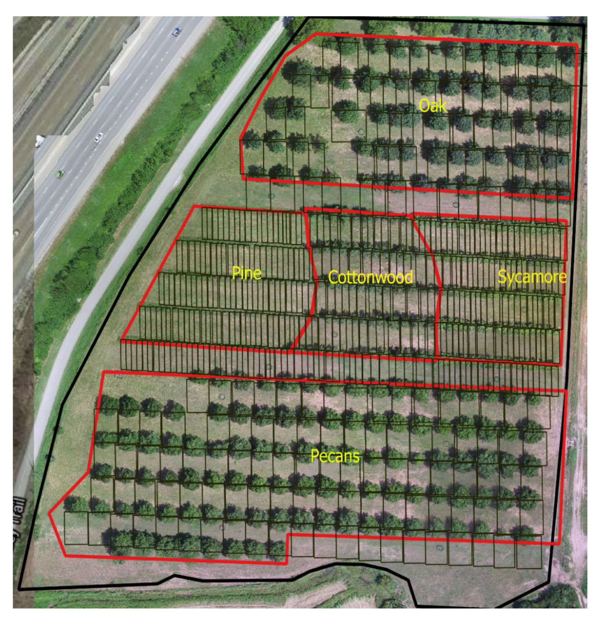
2.1. Site and Experiment Description

The study was located on a 4.25-hectare silvopasture site (Figure 1) at the University of Arkansas Agricultural Research and Extension Center in Fayetteville, AR (36.09° N, 94.19° W). Information on previous site history is described by [15,16,17]. Briefly, soil in most of the experimental area is mapped as Captina silt loam (fine-silty, siliceous, active, mesic Typic Fragiudults), Pickwick silt loam (fine-silty, mixed, semiactive, thermic Typic Paleudults), Johnsburg silt loam (fine-silty, mixed, active, mesic Aquic Fragiudults), and Nixa cherty silt loam (loamy-skeletal, siliceous, active, mesic Glossic Fragiudults; Soil Survey Staff, 2019b). A dissimilar inclusion is also present at this site that is lower in elevation and was not captured in the mapping unit [14]. Sixteen rows of three tree species, Northern red oak (Quercus rubra L.), eastern black walnut (Juglans nigra L.), and pecan (Carya illinoinensis Wangenh. K. Koch), were established in 1999–2000 at 15 m row spacing. The eastern black walnut trees were replaced with three tree species; American sycamore (Platanus occidentalis L.), cottonwood (Populus deltoides W. Bartram ex Marshall), and pitch/loblolly pine (Pinus rigida/Pinus taeda) in 2014. Tree row alleys (4.57 m wide) were planted with two forage species; a cool-season species (orchardgrass (Dactylis glomerata L., var. Tekapo)) in fall 2015 and a native warm-season mix (8:1:1 big bluestem (Andropogon gerardii Vitman), little bluestem (Schizachyrium scoparium (Michx. Nash) and indiangrass (Sorghastrum nutans L.)) in spring of 2016. Poultry litter fertility treatment (fertilized at 84 kg N ha−1 vs. a zero rate (control)) was employed per forage treatment in the spring of 2017, 2018, and 2019. A low elevation area with high soil moisture content within the site was delineated as aquic (wet) treatment while the rest of the area was designated as udic (dry) treatment. The site was grazed by heifers (Bos taurus L.) at 2.2 animal units (AU) (2017 and 2018) and 2.4 AU (2019) per hectare during the summer. In summary, this three-year (2017–2019) silvopastoral grazing study evaluated grass treatments (orchardgrass and a native grass mix), tree species (cottonwood, oak, pecan, pine, and sycamore), soil fertility (poultry litter and a control), and soil moisture regimes (udic and aquic).

2.2. Sampling and Processing for Silvopasture Variables

Soil water content (0.33, 1, 3, and 15 bar) and temperature measurements were recorded every 4 h and logged on a Decagon EM50 data logger (METER Group, Pullman, WA) from May to July in 2017–2019. There were 34 sensors total at the site (17 locations and 2 depths). These data were processed to obtain daily average measurement values. Photosynthetically active radiation (PAR) and leaf area index (LAI) were measured every 10 to 15 days using an AccuPAR LP-80 ceptometer (METER, Pullman, WA) throughout the study period. Soil samples (per grass treatment, fertility, and soil moisture regime) were collected in triplicate at the 0 to 15 cm depth each year during the study period (2017–2019). Total C and N were determined using the combustion method, while soil organic matter was determined using the weight loss on ignition (LOI) method. Other soil parameters; soil texture (modified hydrometer method; sand, silt, and clay in percentage), pH and EC (1:10 soil:water extract), soil nutrient concentration (Mehlich-3 method using 1:10 soil:extractant; P, K, Mg, S, Ca, Na, B, Mo, Ni, Al, Se, Fe, As, Cu, Zn, Mn, Pb, Cr, Ti, Cd, and Co) were analyzed on soil samples following appropriate procedures as described in [18,19]. On each plot, soil bulk density was measured using a 4.8 cm diameter core [20].
A grazing exclosure of 4 m2 area was secured per treatment combination (and replicated thrice) to measure accumulated forage, which was measured by clipping 0.75 m2 of uncut forage to a 6 cm stubble height four times during the grazing season. Outside the exclosure (grazed area), available forage was also measured on each sampling date. Forage nutrient content and quality parameters (C, N, lignin, acid detergent fiber (ADF), neutral detergent fiber (NDF), hemicellulose, total ash, water-soluble carbohydrate, forage nutrients, and metals (P, K, Mg, S, Ca, Na, B, Mo, Ni, Al, Se, Fe, As, Cu, Zn, Mn, Pb, Cr, Ti, Cd, and Co)) were determined in both available and accumulated forage biomass as described in [21,22]. Nutrient removal (N, P, and K removal) by forage (both available and accumulated forage) was calculated based on nutrient content and forage yield measurement.
Tree parameters such as diameter at breast height (DBH; diameter at 137 cm above soil level) and tree height measured for each individual tree during 2017–2019 were averaged for the analysis. Each heifer and its grazing activity were recorded using GPS collars (Model 3300LR, Lotek Wireless Inc., Newmarket, ON) during the summer grazing period (2017–2019). These point data represent a grazing event for each 15 min when animals’ heads are down for more than 75% of the time during this interval.
Study site terrain attributes; elevation (m), aspect (°), flow accumulation (FlowAccum, n), slope-length factor (LSFactor, m); midslope position (MidSlope, index), multi-resolution ridge top flatness index (MRRTF, index), multi-resolution valley bottom flatness index (MRVBF, index), normalized height (NormHt, index), slope percent (SlopePer, %), slope height (SlopeHt, m), system for automated geoscientific analysis wetness index (SAGAWI, index), valley depth (ValleyDep, m), soil depth (soildepth, cm), and altitude above channel network (VDistChn, m) were derived from 1m × 1 m DEM as described in Adhikari et al. (2018). [14] used these 1m × 1 m raster images of terrain parameters to classify four similarly behaving areas within the study sites called topographic functional units (TFU), as well as to help explain soil microbial linkages to production zones [23,24].

2.3. Data Preprocessing for Analysis

Individual trees in the study site were assigned a unique ID. Each tree ID was correlated with the treatment information (tree species, forage species, fertility, wetness) based on its location within the study site. Forage grass treatments were planted between the tree alleys; hence non-overlapping tree polygons were created (Figure 1). Soil and forage parameter values that were collected at each treatment combination level (tree species, forage species, fertility, wetness) were also assigned to each tree ID based on their treatment information. A data set without treatment information but with the geo-referenced location was assigned to each treatment combination after evaluating their position with respect to the tree polygons. Terrain attribute values were extracted per tree polygon using “raster” [25] packages in R [26]. Terrain attributes per tree polygons were averaged for numeric variables, while the most frequent value (mode) was used to extract TFU information per polygon.
For each year, the number of grazing data points were counted per polygon with the collar ID (individual animal) information. Each collar GPS point represents a 15 min grazing interval. Collar GPS data recorded outside of the study area and/or with a dilution of precision greater than four was removed in preprocessing, as was all tilt data with tilt percentage less than 70% in the previous five minutes. Thereafter, the total number of grazing events per polygon was converted to total grazing hours per hectare per AU using polygon area and number of animals (collar ID) information. A combined data set (tree, forage, soil, terrain attributes, and grazing events) containing a total of 130 variables was then created. Tree species, forage species, fertility (poultry manure), wetness, and TFU were categorical variables, while the remaining 125 variables were numerical.

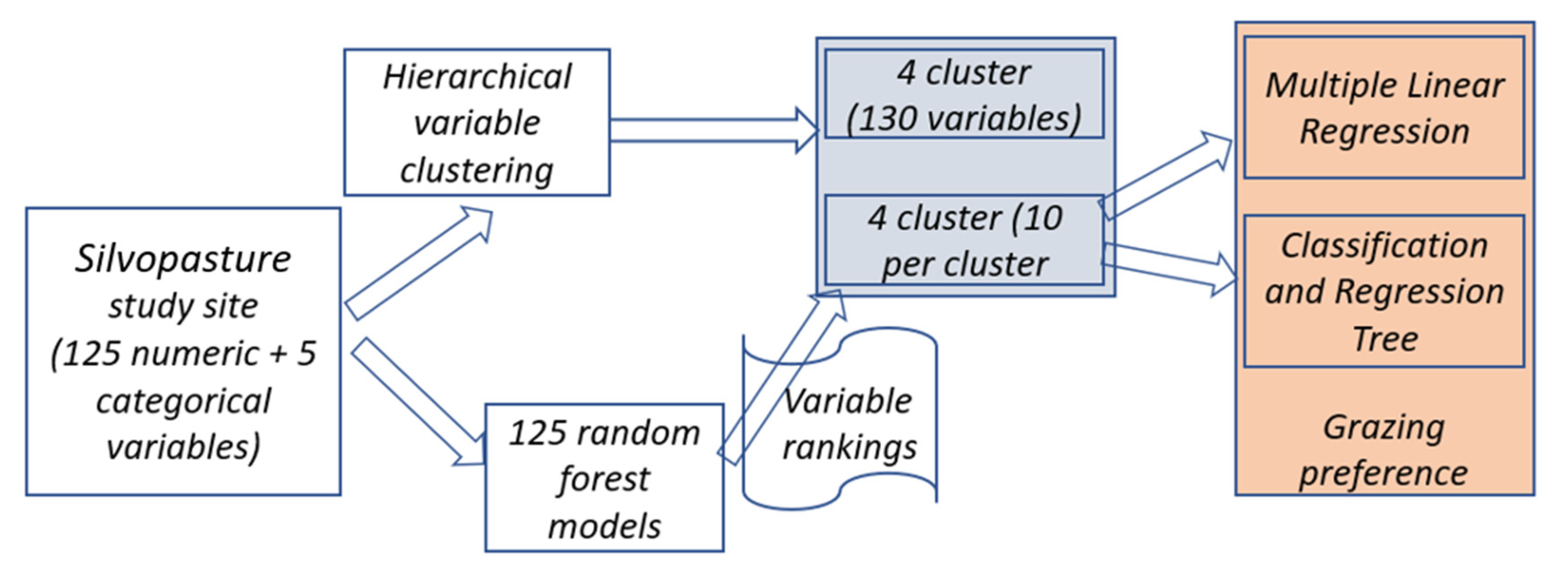
2.4. Machine Learning Approach to Identify Important Variables in a Silvopasture System

2.4.1. Grouping Similar Variables Using Hierarchical Variable Clustering

Silvopasture systems are diverse and complex, where several interacting factors influence the system output. Clustering variables with similar information allows for the identification of important variables to further explore how each of those factors influences the system output. Hierarchical variable clustering (HVC) involves calculating dissimilarity between variables and applying a clustering algorithm iteratively until similar variables group together. The goal is to maximize intra-cluster similarity and minimize inter-cluster similarity. This measure of similarity is defined by the first principal component of the cluster and its correlation/association with the variables within the cluster [27]. Variables are then assigned to those clusters with the highest association values. The algorithm stops once there is no more change in the variable partition to the clusters. Dendrograms visualize the hierarchy of the clusters and help to decide/choose the final number of clusters. The cluster stability is evaluated by bootstrap resampling and then applying the Rand index [28] that penalizes false positive and false negative decisions on the generated clusters.
Variable clustering was performed using the “ClustOfVar” [27] package in R. The approach in this package uses the HVC algorithm for both quantitative and qualitative variables to group them in clusters based on their similarity and association within the cluster. For qualitative variables, correlation ratios of the variable with the first principal component of the cluster were used, while for quantitative variables, squared Pearson correlation coefficients were used. After the clustering algorithm was applied to all 130 variables, a cluster dendrogram was produced. Dendrograms help visualize how each of the variables was grouped and linked together. Four major clusters (Figure 2) were selected based on visual inspection of the cluster dendrogram [27]. Finally, variables per cluster, as well as the score of each variable loading with the cluster (indicating the strength of association), were generated (Table 1).

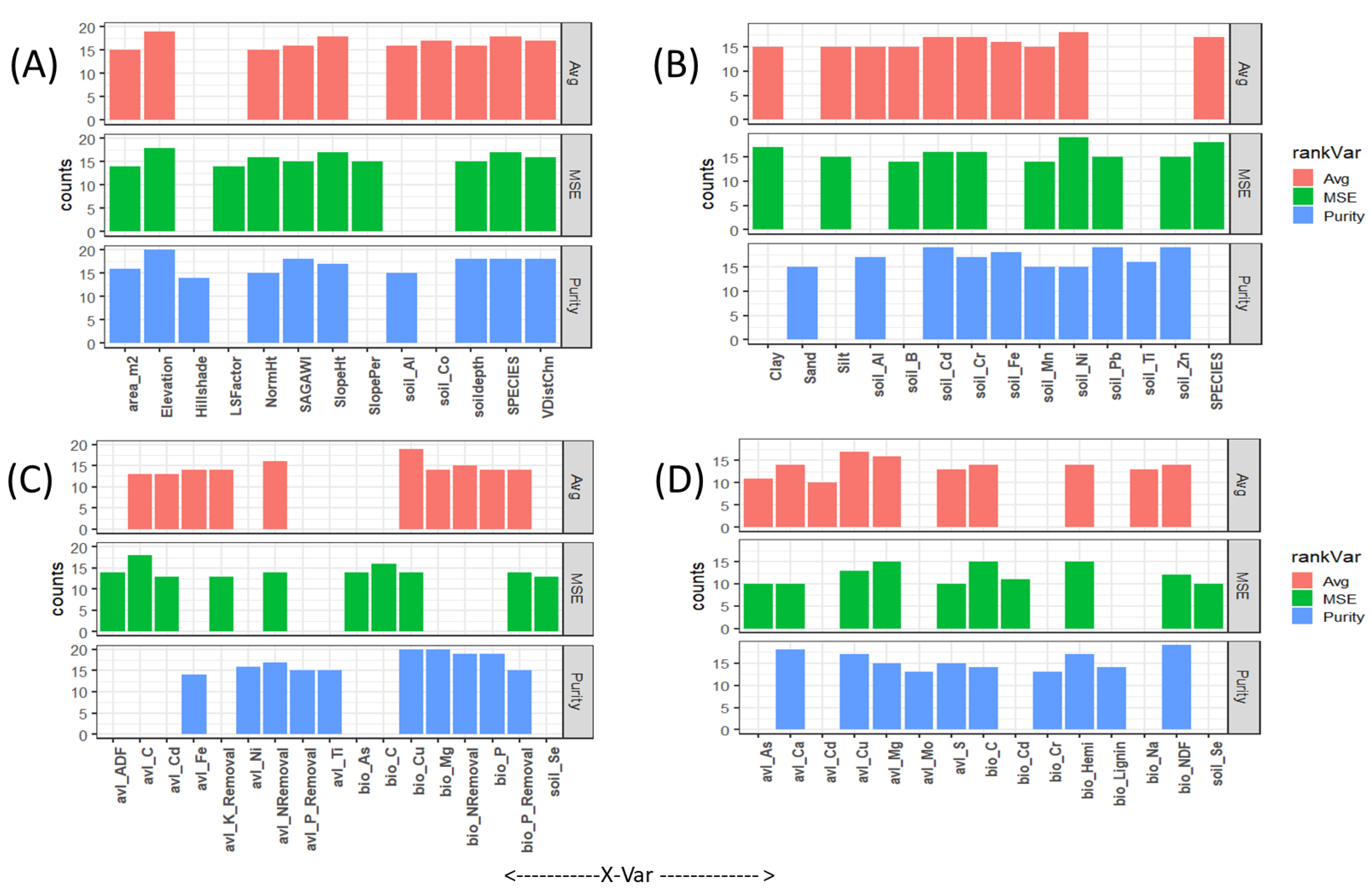
2.4.2. Variable of Importance Using Random Forest Model

Random forest [29] is a non-parametric, machine learning approach where ensembles of classification and regression tree predictions are averaged to make the final prediction model [30]. The CART is a recursive binary split method of input space. In the case of regression predictions, CART decides the best split node by minimizing the sum of squared deviations between each response and the mean predicted value for the node. This approach is useful when there are large numbers of explanatory variables because of its capacity to handle nonlinear relationships and interactions among predictor variables. Individual trees are grown by randomly resampling (with replacement) the training data (called bootstrap sample), as well as using the subset of explanatory variables at a time, which is called the random subspace method. Bagging [30] is the process of the aggregating model developed by the bootstrap sample. Out-of-bag (OOB) mean square error (MSE)of the RF model is the mean prediction error calculated from the training data set when each particular observation was not present in the bootstrap sample.
The random forest algorithm uses two criteria to assess the importance of the selected variables. First, important variables in the models are ranked by an estimate of the decrease in predictive accuracy when the variable is not included in the prediction model. The second measure is ranking variables by their contribution to node (splitting node) purity by using the random subset of variables. Averaged over all regression trees, a decrease in residual sum of square (RSS) by the variables in question allows measurement of this indicator.
The RF models were developed to predict each of the 125 quantitative variables (response variable, y) separately using the R package “randomForest” [31]. For each of the RF model response variable (y), the remaining 129 variables (130 variables less response variable) were used as explanatory variables.
y i = X i
where y i is the ith response variable and X i is the matrix of 129 variables other than the ith response variable. Random forest parameters: nTree (number of trees to grow each time) was set to 500, and mTry (number of variables needed at each node/split) was set to 43.
Each RF model produced important variables based on increases in MSE and increases in node purity. Variables were ranked highest to lowest based on these two criteria. A column with the average ranking of these two criteria was also developed. Next, the twenty most important variables for each model were selected using: (1) MSE ranking, (2) node purity ranking, and (3) average ranking of MSE and node purity. Each RF model then grouped response variables into one of the four clusters. Finally, for each group (cluster), the 10 most frequently occurring ranked variables were selected (Figure 2 and Figure 3). Variables selected using this new approach, “variable ranking” was compared with the standard hierarchical clustering output.

2.5. Animal Grazing Preference Modeling Using Variables Selected by RF-Based Variable Ranking Method

Selected variables based on the averaged ranking method were used to predict animal grazing preference. Summer active grazing hour per ha per AU (labeled as “grz_hr_ha”) was averaged for all 3 years (2017, 2018, and 2019) for this study. The random forest variable selection method described previously resulted in 10 variables per cluster that were important for system-level analysis. These 40 variables (10 per cluster) were selected to model grazing preference using two approaches: MLR method and the CART method. Outputs from these two methods were compared for the grazing preference interpretation. For MLR, a stepwise regression using both backward and forward selection methods was employed to select important variables using the “MASS” package [32] in R. A final MLR model was thus summarized for each selected variable with its coefficient and variance inflation ratio (VIF) to assess if some of these variables still contained redundant information. For CART, a regression tree for the grazing hour was developed using all 40 variables selected by the average ranking method. The R package “rpart” [33] was used for the CART model. The default parameter controls of the “rpart” package were used to develop grazing hour prediction models, where a minimum number of observations needed to attempt a split node was set to 20, the minimum number of observations in any terminal node/leaf was set to 7, complexity parameter (for additional split, R2 value must increase by) to 0.01, and 10-fold cross-validation was used. The algorithm develops fully grown trees at first and then prunes the trees based on control parameters for the final model output.

3. Results

3.1. Grouping Variables Together Using Hierarchical Clustering Method

A total of 130 variables were clustered into four broad groups (Table 1). The majority of variables were in cluster one, along with nearly all terrain features, indicating terrain features are an important factor driving the majority of variability in the silvopasture data set. Tree species and the terrain feature SAGAWI were most strongly correlated with this cluster, along with other terrain features (normalized height, slope percent, slope height, soil depth, MRVBF, and hillshade). Among other strongly correlated variables in this group were tree coverage area as represented by area_m2, soil water content (at 1 bar), and volumetric water content. In summary, this cluster represented terrain features, soil water content, and tree species and tree area (coverage area) of the site. The second group (cluster 2) was composed primarily of soil parameters and was strongly correlated with soil metals such as soil Cd, Cr, Pb, Ti, Cu, As, Fe, and Al (Table 1). Soil texture and soil pH were also grouped within the second cluster.
The third and fourth groups were composed of forage parameters. Two sets of forage samples, accumulated biomass (labeled as “bio”) and available forage mass (labeled as “avl”), were distinctly separated within these two groups. Forage nutrient content (i.e., N, P, and K) and fertilizer application were strongly correlated in cluster three, while forage structural parameters such as NDF, hemicellulose, lignin, and forage species were correlated with cluster four.

3.2. Important Variables Using Random Forest Method

In general, strongly correlated variables for each cluster also appeared as important variables based on RF models (Figure 3 and Table 1). For example, tree species, SAGAWI, and NormHt variables that were strongly correlated with cluster one also appeared as important variables (repeatedly appeared in RF models) for this cluster. The most strongly related variables per cluster (Table 1), for example, tree species (SPECIES, cluster 1), soil Cd (cluster 2), P removal by accumulated biomass (cluster 3), and NDF content of accumulated biomass (cluster 4), were selected by both node purity and MSE method (Figure 3). However, there were differences in selected variables based on MSE and node purity method. Variable selection using either MSE or node purity resulted in 8/10 same variables for cluster one (tree coverage area, elevation, normalized height, SAGAWI, slope height, soil depth, tree species, and altitude above channel network; Figure 3A), 7/10 same variable for cluster four (available forage Ca, Cu, Mg, and S content, accumulated biomass C, hemicellulose, and NDF content; Figure 3D) and 6/10 same variables for cluster two (soil Cd, Cr, Mn, Ni, Pb, and Zn content; Figure 3B). MSE and node purity method selected only 3/10 same variables in cluster three (N removal by available forage, accumulated biomass Cu content, and P removal by accumulated biomass; Figure 3C). The node purity algorithm selects variables to minimize the sum of squares based on the splitting of each node, while MSE selects variables based on predictive accuracy. To capture the importance of both criteria, an averaged ranking (MSE ranking and node purity ranking) method was also used to select the variables (Figure 3).
Using the average method (average of MSE and node purity ranking), the majority of explanatory variables selected to model response variables in each cluster were from the same cluster. For example, except for soil Al, all other selected variables for cluster 1 (Figure 3A) were from the same cluster (Table 1). Similarly, except clay and tree species, all other variables selected for cluster 2 were from the same cluster. Tree species appeared in both clusters (cluster 1 and cluster 2, Figure 3A,B), indicating it is one of the important variables to explain several system-level processes and interrelationships. Variables selected in cluster 3 were entirely from the same cluster. For cluster 4, except Cd content in available forage mass, all other variables selected were from the same cluster. Although several of the selected variables were from the same cluster, the RF variable ranking method showed that variables that were weakly correlated with respective clusters (variables showing <0.5 scores in Table 1) were important enough to explain some system-level interrelationships.

3.3. Linear Regression-Based Interpretation of Selected Variables for Animal Grazing Preference

Summer grazing hour was highly variable with a mean of 77.7 and standard deviation of 56 h ha−1 AU−1 but indicated grazing preference varied by tree species (Table 2). However, stepwise linear regression was unable to determine the importance of tree parameters (species, area coverage) on grazing pressure. Variables were grouped into terrain attributes, soil parameters, and forage parameters (Table 2). Based on the linear regression coefficient, grazing hour decreased (negative coefficients) with slope height, soil Ni, soil Cr, soil Mn, and accumulated biomass Cu and P content. Similarly, grazing hour increased (positive coefficients) with SAGA wetness index, normalized height, soil Cd, soil Fe, and N removal, Fe, C, and Ca content of available forage mass.
For this study, based on a digital elevation model and random forest algorithm, SAGAWI, ValleyDep, and SlopeHt were the main contributing terrain attributes explaining soil nutrient spatial distribution and dynamics. Similar important terrain attribute variables (SlopeHt, SAGAWI, and NormHt), as well as additional soil and forage parameters, were important for explaining animal grazing preferences.

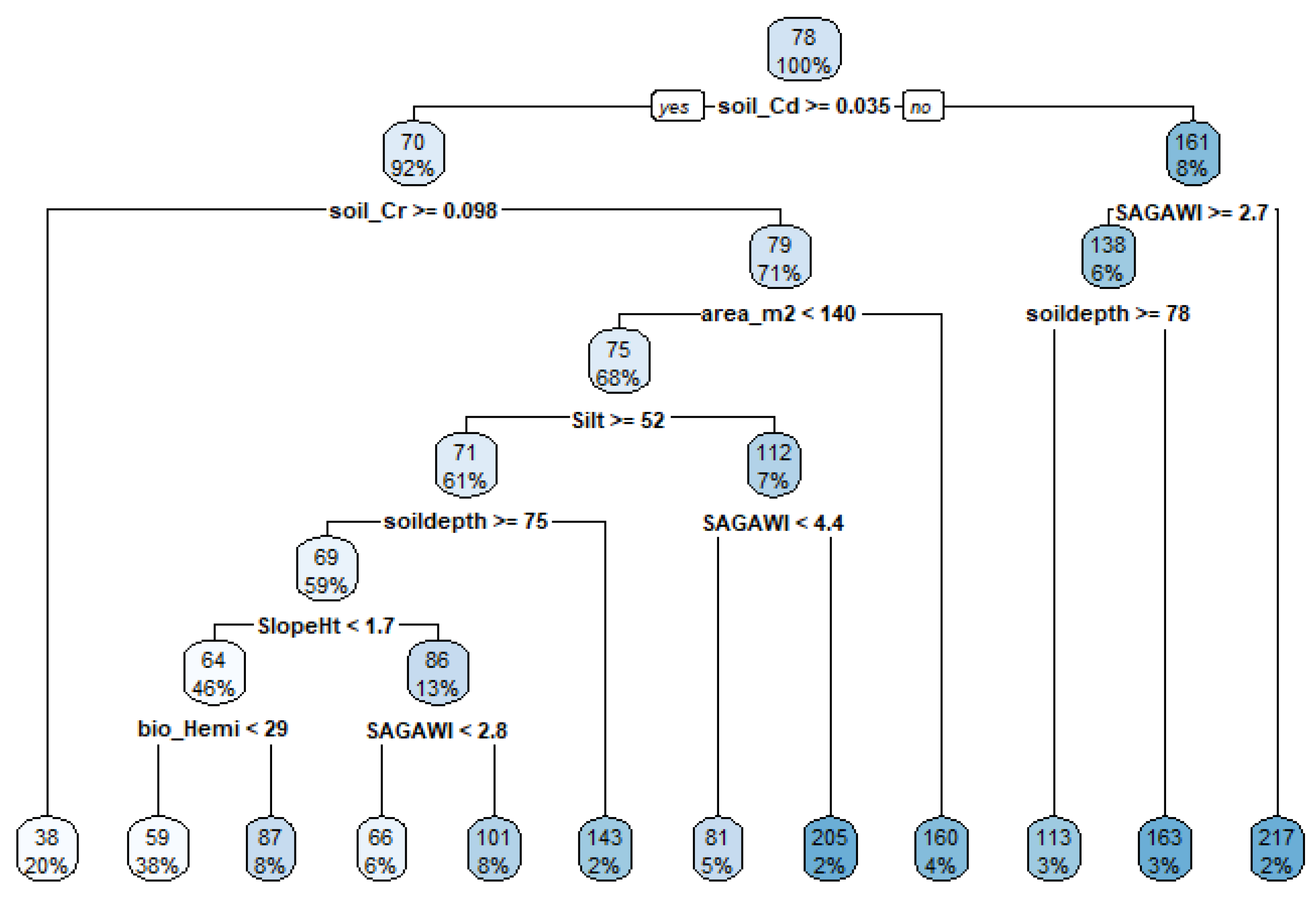
3.4. CART-Based Interpretation of the Selected Variables for Grazing Preference

Soil metals Cd and Cr, and terrain attributes SAGA wetness index and tree coverage area were important variables for identifying factors affecting grazing preference, as selected by the CART method (Figure 4). Soil Cd appeared decisive to split the whole data set into two groups of animal grazing hour: 70 and 161 h ha−1 AU1. Fewer grazing hours (71 h ha−1 AU−1) were associated with soil Cd ≥ 0.035 mg kg−1, and the majority of data (92% data) were under this group. The inference drawn from this result and the linear regression model output (Table 2) were different. The positive coefficient of soil Cd in linear regression suggested grazing hour increased with higher soil Cd, while the CART model showed the opposite result. We further explored soil Cd and its relationship with forage parameters (both accumulated forage biomass and available forage, data not shown), and results suggested that forage yield, NDF, and ADF decreased with increasing soil Cd contents at this site. Soil Cd itself was influenced by experimental factors (tree species, fertilizer application, wetness, and grass treatments) and was usually higher in the aquic (wet), un-fertilized areas where orchardgrass was grown (Table 3). Therefore, animals preferred grazing native grasses (53.9 vs. 101 h ha−1 AU−1) and udic (dry) areas (51.8 vs. 103.2 h ha−1 AU−1), where soil Cd content was significantly lower (Table 3).
Terrain attribute SAGA wetness index was another important variable selected by the CART method to explain animal grazing preference (Figure 4). This variable appeared repetitively on the CART node to delineate animal grazing preference. Higher SAGAWI values infer pixels where water would accumulate following a rainfall event indicating lower elevation area within the study site with comparatively more wetness. In general, a higher value (more wetness) was associated with fewer animal grazing hours. On average, sites with the SAGAWI ≥2.7 showed 138 h ha−1 AU−1 grazing hour compared to 217 h ha−1 AU−1 when SAGAWI was less than 2.7. Again, compared to a linear regression (Table 2) approach where SAGAWI showed a positive coefficient value, the CART interpretations were different and more realistic.
Soil Cr was another statistically significant variable selected by CART and stepwise linear regression methods. Similar to soil Cd, higher soil Cr (≥0.09 mg kg−1) was associated with fewer animal grazing hours (Figure 4; 38 vs. 79 h ha−1 AU−1). The linear regression (Table 2) method also showed a negative slope coefficient for the soil Cr to predict animal grazing hours. Similar to soil Cd, Cr was higher in wet, un-fertilized, and areas where orchardgrass was grown (Table 3).
The tree coverage area represents the areal area coverage of each individual tree within the study site. Higher area coverage represents larger trees compared to lower area coverage. Area coverage appeared in the CART approach as an important variable (Figure 4); however, it did not appear in the stepwise linear regression method (Table 2). Animals preferred grazing (160 vs. 75 h ha−1 AU−1) where trees were larger (tree coverage 140 m2 or more). Table 3 shows that tree coverage was not affected by any factor other than tree species. Larger trees (greater diameter at breast height) within the sites were pecan (132 m2), and animals preferred grazing (103 h ha−1 AU−1) on these sites. However, results also indicated that smaller trees did not always result in fewer grazing hours. Pine trees, for example, were the smallest trees on the study site (28.8 m2 tree coverage), and animals preferred grazing there compared to sycamore (Table 3; 80.8 vs. 58.5 h ha−1 AU−1). Other factors that appeared in the CART approach, such as silt content, soil depth, slope height, and hemicellulose, were determinants for further variation in animal grazing preference.
In general, greater silt content (equal or greater than 52%) was linked to lower animal grazing hours (Figure 4; 71 vs. 112 h ha−1 AU−1). Similarly, greater soil depth (equal to or greater than 75 cm) was associated with less grazing (69 vs. 143 h ha−1 AU−1). Animal grazing hour was greater (86 vs. 64 h ha−1 AU−1) under greater slope height (slope height equal to or greater than 1.7). Finally, hemicellulose content greater than 29% was associated with greater grazing (87 vs. 59 h ha−1 AU−1).

4. Discussion

The authors used a variable ranking method to select important variables for the system-level analysis. Compared to cluster analysis, some of the selected variables (by variable ranking method) came from different cluster groups. Although not all, most of the strongly correlated variables (Table 1; variables with higher loading score) were selected by our variable ranking approach (Figure 3). This result helped to conclude that the new approach was comparable to HVC for variable selection and helpful to reduce a large number of variables into a few important ones for system-level analysis.
Selected variables were used to develop a grazing preference model using a machine learning approach CART and MLR. As discussed by [12,13], the limitation of MLR due to linearity assumption and autocorrelation (correlation between independent variable) was evident. We used variables with VIF <10 to select less correlated variables during MLR (Table 2), still the interpretation of MLR output was different from the machine learning approach (CART), probably due to linearity limitation. For example, with higher soil Cd content and SAGAWI, animal grazing hours increased (Table 2) in MLR while it decreased in CART (Figure 4). The interaction of SAGAWI with other variables was evident on the CART model, as it appeared repeatedly with different coefficient values (Figure 4) on different nodes. Factor-level analysis and comparison of model coefficient (MLR and CART) with ANOVA showed that CART performed better than MLR for explaining the relationship of selected variables with the response variable grazing preference.
Animal grazing was linked primarily with soil Cd, soil Cr, tree coverage area (areal coverage), and the terrain feature SAGAWI. Cattle preferred grazing locations with lower SAGAWI (drier areas), native forages, and lower soil Cd and Cr contents. A comparison with ANOVA results (Table 3) also confirmed that these drier sites (with lower SAGAWI, soil Cd, and soil Cr contents) had greater animal grazing hours.
In summary, cattle grazing preference is influenced by the interaction of plant, animal, and environmental factors [34]. Cattle respond to these factors by selecting plants or plant parts with the most desirable nutritive value [35]. We found soil metals Cd, Cr, and terrain attributes SAGA wetness index to be the most important factors influencing animal grazing preference in our study. [14] reported SAGAWI as one of the important terrain attributes determining soil nutrient distribution on this site. Cattle grazing preference and its relationship with the lower metal content of the site is related to the water movement due to landscape position, as indicated by the SAGA wetness index. Greater soil metals (Cd and Cr) were associated with lower elevation areas within the site. Several studies report landscape hydrology as a function of terrain attributes [36,37,38,39] that ultimately drives the nutrient and metal distribution. Soil Cd increased with SAGAWI (regression coefficient, b = 0.009) and soil depth (b = 0.001), while it decreased with the elevation (b = −0.003) within the site (DNS). Soil Cr showed a similar relationship with SAGAWI, soil depth, and elevation, indicating the occurrence of these metals was likely more of a function of terrain attributes and concentration of these metals were higher on lower elevation and depressional area. [40] also reported that higher soil Cd was associated with lower elevation topographic areas within a Northern Great Plains study site. Forage yield (both accumulated biomass and available forage mass) decreased with increasing soil Cd and Cr content in our study (DNS); hence, lower animal grazing hours are expected with less forage availability on these depression areas.

5. Conclusions

Silvopastoral system components, including grass and tree species, and their interaction with terrain-associated factors require a multi-variable approach to understand system-level functionality. We hypothesize that the machine learning approach will help to improve both variable selection and factor-level interpretation for a complex system with multiple interacting variables. A three-year (2017–2019) silvopastoral grazing study was used to evaluate a novel approach called “variable rankings” to select most important variables using the machine learning RF method. Results showed that this new approach was comparable to HVC for variable selection and was helpful in reducing a large number of variables into a few important ones for system-level analysis. Selected variables were then used to develop an animal grazing preference model using machine learning (CART) and MLR approach. Machine learning model CART showed a better cause-effect relationship with the animal grazing preference compared to the MLR. Based on the CART result, animal grazing was linked primarily by soil Cd, soil Cr, tree coverage area, and the terrain feature SAGAWI. Cattle preferred grazing locations with lower SAGAWI (drier areas), native forage mixture, and lower soil Cd and Cr contents. A comparison with ANOVA results also confirmed that these drier sites (with lower SAGAWI, soil Cd, and soil Cr contents) had greater animal grazing hours. A machine learning-based variable ranking approach used in this study helped to subset important variables that can be used for statistical inference. In conclusion, animal grazing preference was influenced by tree species (larger pecan trees preferred), grass treatments (native grass preferred), soil, and landscape attributes, and may help explain pasture use. Machine learning is a viable approach for identifying systems-level drivers of a complex silvopasture system.

Author Contributions

Conceptualization, T.P.K.; methodology, T.P.K.; software, T.P.K.; validation, A.J.A., P.R.O., D.P., A.L.T., and T.J.S.; formal analysis, T.P.K.; investigation, T.P.K., A.J.A., P.R.O., D.P., A.L.T., and T.J.S.; resources, A.J.A., P.R.O., D.P., A.L.T., and T.J.S.; data curation, T.P.K.; writing—original draft preparation, T.P.K.; writing—review and editing, T.P.K., A.J.A., P.R.O., D.P., A.L.T., and T.J.S.; visualization, T.P.K.; supervision, A.J.A.; project administration, A.J.A.; funding acquisition, A.J.A. All authors have read and agreed to the published version of the manuscript.

Funding

This research was made possible by a USDA-ARS Big Data funding opportunity.

Institutional Review Board Statement

The study was conducted according to the guidelines of the Declaration of Helsinki, and approved by the Institutional Review Board (Institutional Animal Care and Use Committee) of University of Arkansas (Protocol code 19079 and date of approval 9 May, 2019).

Informed Consent Statement

Not applicable.

Data Availability Statement

The data presented in this study are available on request.

Acknowledgments

Trade names or commercial products mentioned in this article are solely for the purpose of providing specific information and do not infer either recommendation or endorsement by the U.S. Department of Agriculture. Field management by Robert Rhein with the University of Arkansas Animal Science Department and Taylor Adams with the USDA-ARS is gratefully acknowledged.

Conflicts of Interest

The authors declare that there is no conflict of interest.

Abbreviations

ADF, acid digestible fiber; AU, animal units; C, carbon; CART, classification and regression tree; DBH, diameter breast height; DNS, data not shown; GPS, global positioning system; HVC, Hierarchical variable clustering; LAI, leaf area index; LOI, loss in ignition; MLR, multiple linear regression; MSE, mean square error; NDF, neutral detergent fiber; OM, organic matter; OOB, out of bag; PAR, photosynthetically active radiation; RF, random forest; RSS, residual sum of squares; SOC, soil organic carbon; VIF, variance inflation ratio; VWC, volumetric water content.

References

  1. Cardinael, R.; Chevallier, T.; Cambou, A.; Béral, C.; Barthès, B.G.; Dupraz, C.; Durand, C.; Kouakoua, E.; Chenu, C. Increased soil organic carbon stocks under agroforestry: A survey of six different sites in France. Agric. Ecosyst. Environ. 2017, 236, 243–255. [Google Scholar] [CrossRef] [Green Version]
  2. Pinho, R.C.; Miller, R.P.; Alfaia, S.S. Agroforestry and the improvement of soil fertility: A view from Amazonia. Appl. Environ. Soil Sci. 2012, 2012, 616383. [Google Scholar] [CrossRef]
  3. Jose, S. Agroforestry for ecosystem services and environmental benefits: An overview. Agrofor. Syst. 2009, 76, 1–10. [Google Scholar] [CrossRef]
  4. Schroeder, P. Agroforestry systems: Integrated land use to store and conserve carbon. Clim. Res. 1993, 3, 53–60. [Google Scholar] [CrossRef]
  5. Bzdok, D.; Altman, N.; Krzywinski, M. Statistics versus machine learning. Nat. Methods 2018, 15, 233–234. [Google Scholar] [CrossRef]
  6. Samuel, A.L. Some studies in machin learning using the game of checkers. IBM J. Res. Dev. 1959, 3, 210–229. [Google Scholar] [CrossRef]
  7. Cioffi, R.; Travaglioni, M.; Piscitelli, G.; Petrillo, A.; De Felice, F. Artificial intelligence and machine learning applications in smart production: Progress, trends and directions. Sustainability 2020, 12, 492. [Google Scholar] [CrossRef] [Green Version]
  8. John, G.H.; Langley, P. Static versus dynamic sampling for data mining. In Proceedings of the Second International Conference on Knowledge Discovery and Data Mining; AAAI Press: Portland, OR, USA, 1996. [Google Scholar]
  9. Georganos, S.; Grippa, T.; Vanhuysse, S.; Lennert, M.; Shimoni, M.; Kalogirou, S.; Wolf, E. Less is more: Optimizing classification performance through feature selection in a very-high-resolution remote sensing object-based urban application. GIScience Remote Sens. 2018, 55, 221–242. [Google Scholar] [CrossRef]
  10. Bzdok, D. Classical statistics and statistical learning in imaging neuroscience. Front. Neurosci. 2017, 11, 543. Available online: https://www.frontiersin.org/articles/10.3389/fnins.2017.00543/full (accessed on 18 July 2021). [CrossRef]
  11. Wang, S.; McCormick, T.H.; Leek, J.T. Methods for correcting inference based on outcomes predicted by machine learning. Proc. Natl. Acad. Sci. USA 2020, 117, 30266–30275. [Google Scholar] [CrossRef]
  12. Morr, P.E. Age of acquisition, imagery, recall, and the limitations of multiple-regression analysis. Mem. Cogn. 1981, 9, 277–282. [Google Scholar] [CrossRef] [Green Version]
  13. Porter, A.L.; Connolly, T.; Heikes, R.G.; Park, C.Y. Misleading indicators: The limitations of multiple linear regression in formulation of policy recommendations. Policy Sci. 1981, 13, 397–418. [Google Scholar] [CrossRef]
  14. Adhikari, K.; Owens, P.R.; Ashworth, A.J.; Sauer, T.J.; Libohova, Z.; Richter, J.L.; Miller, D.M. Topographic controls on soil nutrient variations in a silvopasture system. Agrosystems Geosci. Environ. 2018, 1, 180008. [Google Scholar] [CrossRef]
  15. Sauer, T.J.; Coblentz, W.K.; Thomas, A.L.; Brye, K.R.; Brauer, D.K.; Skinner, J.V.; Brahana, J.V.; DeFauw, S.L.; Hays, P.D.; Moffitt, D.C.; et al. Nutrient cycling in an agroforestry alley cropping system receiving poultry litter or nitrogen fertilizer. Nutr. Cycl. Agroecosystem 2015, 101, 167. [Google Scholar] [CrossRef]
  16. DeFauw, S.L.; Brye, K.R.; Sauer, T.J.; Hays, P. Hydraulic and physiochemical properties of a hillslope soil assemblage in the Ozark highlands. Soil Sci. Soc. Am. J. 2014, 179, 107–117. [Google Scholar] [CrossRef]
  17. Thomas, A.L.; Brauer, D.K.; Sauer, T.J.; Coggeshall, M.V.; Ellersieck, M.R. Cultivar influences early rootstock and scion survival of grafted black walnut. J. Am. Pomol. Soc. 2008, 62, 3–12. [Google Scholar]
  18. Ashworth, A.J.; Kharel, T.; Sauer, T.; Adams, T.C.; Philipp, D.; Thomas, A.; Owens, P.R. Spatial Monitoring Technologies for Coupling the Soil-Plant-Water-Animal Nexus. Sci. Rep. 2021. in review. [Google Scholar]
  19. Ashworth, A.J.; Adams, T.C.; Kharel, T.P.; Philipp, D.; Owens, P.R.; Sauer, T.J. Root Decomposition in Silvopastures is Influenced by Grazing, Fertility, and Grass Species. Agrosystems Geosci. Environ. 2021. [Google Scholar] [CrossRef]
  20. Blake, G.R.; Hartge, K.H. Bulk density. In Methods of Soil Analysis, Part 1—Physical and Mineralogical Methods, 2nd ed.; Agronomy Monograph, 9; Klute, A., Ed.; American Society of Agronomy—Soil Science Society of America: Madison, WI, USA, 1986; pp. 363–382. [Google Scholar]
  21. Niyigena, V.; Ashworth, A.J.; Nieman, C.; Achara, M.; Coffey, K.P.; Philipp, D.; Meadors, L.; Sauer, T.J. Factors affecting sugar accumulation and fluxes in warm- and cool-season forages grown in a silvopastoral system. Agronomy 2021, 11, 354. [Google Scholar] [CrossRef]
  22. Dhakal, M.; West, C.P.; Villalobos, C.; Sarturi, J.O.; Deb, S.K. Trade-off between nutritive value improvement and crop water use for alfalfa-grass system. Crop Sci. 2020, 60, 1711–1723. [Google Scholar] [CrossRef] [Green Version]
  23. Gurmessa, B.; Ashworth, A.J.; Yang, Y.; Savin, M.; Moore, P.A., Jr.; Ricke, S.; Pedretti, G.C.E.F.; Cocco, S. Variations in bacterial community structure and antimicrobial resistance gene abundance in cattle manure and poultry litter. Environ. Res. 2021, 197, 111011. [Google Scholar] [CrossRef]
  24. Gurmessa, B.; Ashworth, A.J.; Yang, Y.; Adhikari, K.; Savin, M.; Owens, P.R.; Sauer, T.; Pedretti, E.F.; Cocco, S.; Corti, G. Soil bacterial diversity based on management and topography in a silvopastoral system. Appl. Soil Ecol. 2021, 163, 103918. [Google Scholar] [CrossRef]
  25. Hijmans, R.J. Raster: Geographic data analysis and modeling. R package version 2.9-23. 2019. Available online: https://CRAN.R-project.org/package=raster (accessed on 15 December 2020).
  26. R Core Team. R: A Language and Environment for Statistical Computing; R Foundation for Statistical Computing: Vienna, Austria, 2020; Available online: https://www.R-project.org/ (accessed on 10 December 2020).
  27. Chavent, M.; Kuentz-Simonet, V.; Liquet, B.; Saracco, J. ClustOfVar: An R pakage for the clustering of variables. J. Stat. Softw. Am. Stat. Assoc. 2012, 50, 6809. [Google Scholar]
  28. Hubert, L.; Arabie, P. Comparing partitions. J. Classif. 1985, 2, 193–208. [Google Scholar] [CrossRef]
  29. Breiman, L. Random forests. Mach. Learn. 2001, 45, 5–32. [Google Scholar] [CrossRef] [Green Version]
  30. Breiman, L. Bagging predictors. Mach. Learn. 1996, 24, 123–140. [Google Scholar] [CrossRef] [Green Version]
  31. Liaw, A.; Wiener, M. Classification and regression by randomforest. R News 2002, 2, 18–22. [Google Scholar]
  32. Venables, W.N.; Ripley, B.D. Modern Applied Statistics with S, 4th ed.; Springer: New York, NY, USA, 2002; ISBN 0-387-95457-0. [Google Scholar]
  33. Therneau, T.; Atkinson, B. Rpart: Recursive Partitioning and Regression Trees; R package version 4.1-15. 2019. Available online: https://CRAN.R-project.org/package=rpart (accessed on 15 December 2020).
  34. Marten, G.C. The animal -plant complex in forage palatability phenomena. J. Anim. Sci. 1973, 46, 1470–1477. [Google Scholar] [CrossRef]
  35. Willms, W. Spring forage selection by tame Mule deer on Big Sagebrush range, British Columbia. J. Range Manag. 1978, 31, 192–199. [Google Scholar] [CrossRef]
  36. Cambardella, C.A.; Moorman, T.; Novak, J.; Parkin, T.; Karlen, D.; Turco, R.; Konopka, A.E. Field scale variability of soil properties in central Iowa soils. Soil Sci. Soc. Am. J. 1994, 58, 1501–1511. [Google Scholar] [CrossRef]
  37. Brown, D.J.; Clayton, M.K.; McSweeney, K. Potential terrain controls on soil color, texture contrast and grain-size deposition for the original catena landscape in Uganda. Geoderma 2004, 122, 51–72. [Google Scholar] [CrossRef]
  38. Mehnatkesh, A.; Ayoubi, S.; Jalalian, A.; Sahrawat, K.L. Relationships between soil depth and terrain attributes in a semi arid hilly region in western Iran. J. Mt. Sci. 2013, 10, 163–172. [Google Scholar] [CrossRef]
  39. Umali, B.P.; Oliver, D.P.; Forrester, S.; Chittleborough, D.J.; Hutson, J.L.; Kookana, R.S.; Ostendorf, B. The effect of terrain and management on the spatial variability of soil properties in an apple orchard. Catena 2012, 93, 38–48. [Google Scholar] [CrossRef]
  40. Franzen, D.W.; Nanna, T.; Norvell, W.A. A survey of soil attributes in North Dakota by landscape position. Agron. J. 2006, 98, 1015–1022. [Google Scholar] [CrossRef] [Green Version]
Figure 1. Study site with tree species labels (oak, pine, cottonwood, sycamore, and pecans) and area representing the individual tree polygons. Tree polygons extend southbound to identify grass species treatments (planted in tree alleys) associated with each individual tree.
Soilsystems 05 00041 g001
Figure 2. A flow chart of the model building steps used in this study. Each shaded box shows the comparison of two approaches. Hierarchical variable clustering vs. random forest-based variable rankings approach was compared first. Animal grazing preference was then modeled (multiple linear regression vs. classification and regression tree) using the variables selected from the variable rankings method.
Soilsystems 05 00041 g002
Figure 3. Important ten variables selected per cluster based on random forest model using MSE, node purity and average ranking of MSE, and node purity criteria; (A) variables selected for cluster 1, (B) variables selected for cluster 2, (C) variables selected for cluster 3, and (D) variables selected for cluster 4. See Table 1 for the variable description.
Soilsystems 05 00041 g003
Figure 4. Regression tree developed for animal grazing hour based on the selected 40 (10 per cluster) important variables for system-level analysis. See Table 1 for the variable description.
Soilsystems 05 00041 g004
Table 1. Variables selected per cluster using hierarchical clustering methods. Four clusters were decided based on dendrogram visualization. A total of 130 (5 categorical + 125 numerical) variables were classified into one of four clusters. The score is the squared loadings described in [27], and the value indicates how strongly each variable is associated with the cluster.
Cluster 1ScoreCluster 2scoreCluster 3ScoreCluster 4Score
SPECIES0.82soil_Cd0.86bio_P_Removal0.88bio_NDF 0.90
SAGAWI0.77soil_Cr0.85bio_Mg0.83avl_Ca0.90
NormHt0.63soil_Pb0.79bio_P0.80Forage_spp0.87
SlopePer0.61soil_Ti0.70avl_P_Removal0.74avl_Cu0.87
SlopeHt0.60soil_Cu0.69bio_NRemoval 0.68avl_Na0.82
soildepth0.59soil_As0.69avl_Ni0.68avl_Mo0.77
area_m20.57soil_Fe0.66bio_Mo0.67bio_Hemi0.73
MRVBF0.57soil_Al0.62avl_NRemoval 0.66avl_S 0.69
X1b0.55Sand0.61bio_K_Removal0.65bio_Ca0.66
Hillshade0.55soil_Mo0.57bio_Cu0.65bio_S 0.60
VWC10.50soil_Ca0.55avl_Co0.63avl_Mg0.55
TreeHeight0.48soil_Se0.55avl_Fe0.61bio_Na0.55
Wetness0.44pH0.48bio_N0.60avl_Zn0.55
DBH0.44soil_Mn0.45avl_K_Removal0.56bio_Mn0.51
Elevation0.43Silt0.42Fertilizer0.56bio_Lignin 0.50
soil_Co0.39soil_Zn0.40avl_Pb0.56bio_Cd0.46
VDistChn0.35X15b0.40avl_Mn0.56Carb0.43
Clay0.35soil_P0.35avl_Ti0.54bio_Pb0.28
bio_Cr0.33soil_S0.33avl_Al0.54avl_Lignin 0.28
bio_As0.32soil_Ni0.23avl_Yield 0.54bio_Ash 0.24
LOI0.29avl_Hemi 0.21avl_Ash 0.54bio_C 0.22
bio_Se0.28avl_ADF0.20avl_P0.48bio_B 0.21
LSFactor0.28CN0.19avl_Cr0.44bio_Ti0.17
soil_B0.26X0.33b0.13bio_Zn0.40bio_Al0.15
TFU0.26grz_hr_ha0.12bio_Yield0.32bio_Fe0.14
EC0.19soil_Na0.12LAI0.27avl_As0.11
avl_N0.18X3b0.00bio_Co0.27bio_ADF 0.10
N0.18soil_Mg0.00PAR0.25avl_Se0.06
MidSlope0.17soil_K0.00avl_Cd0.23
Aspect0.17 avl_C0.21
ValleyDep0.16 Density0.15
Suagr0.15 bio_Ni0.12
FlowAccum0.14 Temp0.07
C0.10 avl_B0.02
CO20.09
MRRTF0.08
avl_K0.07
bio_K0.06
avl_NDF0.01
Variable description: SAGAWI = system for automated geoscientific analysis wetness index (index); SPECIES = tree species (cottonwood, oak, pecans, pine, sycamore); NormHt = normalized height (index); MRVBF = multi-resolution valley bottom flatness index (index); soildepth = soil depth (cm); SlopeHt = slope height (m); VDistChn = altitude above channel network (m); Elevation = elevation (m); SlopePer = slope percent (%); ValleyDep = valley depth (m); Hillshade = hillshade (°); MidSlope = midslope position (index); LSFactor = slope-length factor (m); Aspect = aspect (°); FlowAccum = flow accumulation (number of pixels, n); MRRTF = multi-resolution ridge top flatness index (index); TFU = topographic functional units (1–4); Wetness = wetness (aquic, udic); area_m2 = area coverage by each tree polygon (m2); DBH= diameter at breast height (m); TreeHeight = tree height (m); Fertilizer = fertility treatment with poultry litter (fertilized, control); grz_hr_ha = animal visits (h ha−1 AU−1); Carb = forage carbohydrate (g kg−1); Forage_Spp = forage grass species treatment (native warm-season mix, cool-season orchardgrass); LAI = leaf area index (index); PAR = photosynthetically active radiation (µmol m−2 s−1); sugar = forage water-soluble carbohydrates (g kg−1); avl_Cr = forage mass chromium (mg kg−1 dry matter); avl_Fe = forage mass iron (mg kg−1); avl_Al = forage mass aluminum (mg kg−1); avl_Pb = forage mass lead (mg kg−1); avl_Ni = forage mass nickel (mg kg−1); avl_B = forage mass boron (mg kg−1); avl_Ti = forage mass titanium (mg kg−1); avl_As = forage mass arsenic (mg kg−1); avl_Ca = forage mass calcium (mg kg−1); avl_Lignin = forage mass lignin (%); avl_Hemi = forage mass hemicellulos (%); avl_NDF = forage mass neutral detergent fiber (%);avl_Co = forage mass cobalt (mg kg−1); avl_Cd = forage mass cadmium (mg kg−1); avl_Yield = available forage mass yield measured every 10 days during the grazing season (kg ha−1); avl_NRemoval = total N removed from soil by forage mass yield (kg ha−1); avl_P_Removal = total P removed from soil by forage mass yield (kg ha−1); avl_K_Removal = total K removed from soil by forage mass yield (kg ha−1); avl_ADF = forage mass acid detergent fiber (%); avl_C = forage mass carbon (%); avl_Zn = forage mass zinc (mg kg−1); avl_Cu = forage mass copper (mg kg−1); avl_P = forage mass phosphorus (mg kg−1); avl_S = forage mass sulfur (mg kg−1); avl_K = forage mass potassium (mg kg−1); avl_N = forage mass nitrogen (%); avl_Mg = forage mass magnesium (mg kg−1); avl_Mo = forage mass molybdenum (mg kg−1); avl_Ash = forage mass ash (%); avl_Se = forage mass selenium (mg kg−1); avl_Na = forage mass sodium (mg kg−1); avl_Mn = forage mass manganese (mg kg−1); bio_Cr = accumulated bimass chromium (mg kg−1 dry matter); bio_Fe = accumulated biomass iron (mg kg−1); bio_Al = accumulated bomass aluminum (mg kg−1); bio_Pb = accumulated biomass lead (mg kg−1); bio_Ni = accumulated biomass nickel (mg kg−1); bio_B = accumulated biomass boron (mg kg−1); bio_Ti = accumulated biomass titanium (mg kg−1); bio_As = accumulated biomass arsenic (mg kg−1); bio_Ca = accumulated biomass calcium (mg kg−1); bio_Lignin = accumulated biomass lignin (%); bio_Hemi = biomass hemicellulos (%); bio_NDF = accumulated biomass neutral detergent fiber (%);bio_Co = accumulated biomass cobalt (mg kg−1); bio_Cd = accumulated biomass cadmium (mg kg−1); bio_Yield = accumulated biomass yield collected inside grazing exlosure areas every 10 days during the grazing season (kg ha−1); bio_NRemoval = total N removed from soil by accumulated biomass yield (kg ha−1); bio_P_Removal = total P removed from soil by accumulated biomass yield (kg ha−1); bio_K_Removal = total K removed from soil by accumulated biomass yield (kg ha−1); bio_ADF = accumulated biomass acid detergent fiber (%); bio_C = accumulated biomass carbon (%); bio_Zn = accumulated biomass zinc (mg kg−1); bio_Cu = accumulated biomass copper (mg kg−1); bio_P = accumulated biomass phosphorus (mg kg−1); bio_S = accumulated biomass sulfur (mg kg−1); bio_K = accumulated biomass potassium (mg kg−1); bio_N = accumulated biomass nitrogen (%); bio_Mg = accumulated biomass magnesium (mg kg−1); bio_Mo = accumulated biomass molybdenum (mg kg−1); bio_Ash = accumulated biomass ash (%); bio_Se = accumulated biomass selenium (mg kg−1); bio_Na = accumulated biomass sodium (mg kg−1); bio_Mn = accumulated biomass manganese (mg kg−1); soil_Co = soil cobalt (mg kg−1 soil); VWC1 = volumetric water content (m3/m3 soil); soil_Mg = soil magnesium (mg kg−1); X1b = gravimetric water conent at 1 bar (g g−1); soil_Ni = soil nickel (mg kg−1); soil_B = soil boron (mg kg−1); CN = soil carbon:nitroen (ratio); Temp = soil temp at 0–15 cm (°C); EC = soil electrical conductivity (dS m−1); soil_S = soil sulfur (mg kg−1); soil_K = soil potassium (mg kg−1); X15b = gravimetric water content at 15 bar (g g−1); soil_Na = soil sodium (mg kg−1); Sand = sand (%); Silt = silt (%); Clay = clay (%); X3b = gravimetric water content at 3 bar (g g−1 soil); X0.33b = gravimetric water content at 0.33 bar (g g−1 soil); CO2 = soil respiration CO2 (umol cm−1 s−1); Density = bulk density (kg m−3); soil_Cd = soil cadmium (mg kg−1); soil_Ti = soil titanium (mg kg−1); soil_Cr = soil chromium (mg kg−1); soil_Pb = soil lead (mg kg−1); soil_Cu = soil copper (mg kg−1); soil_As = soil arsenic (mg kg−1); soil_Fe = soil iron (mg kg−1); soil_Se = soil selenium (mg kg−1); soil_Al = soil aluminum (mg kg−1); soil_Ca = soil calcium (mg kg−1); soil_Mo = soil molybdenum (mg kg−1); pH = soil pH; soil_Zn = soil zinc (mg kg−1); LOI = soil organic matter measured using loss in ignition method (%); N = soil nitrogen (%); C = soil carbon (%); soil_P = soil phosphorus (mg kg−1); soil_Mn = soil manganese (mg kg−1).
Table 2. Selected variables based on stepwise linear regression to model animal grazing hour, grz_hr_ha (h ha−1 AU−1) with their coefficients and variance inflation factor (VIF). Variables with VIF >10 were removed from the final model. At the bottom, mean, standard deviation and number of observation is summarized for grz_hr_ha variable.
Variables CoefficientANOVA-p > FVIF
Intercept −4025 -
SlopeHt −34 *0.006.8
SAGAWI 12.0 *0.003.8
NormHt 242 *0.009.7
soil_Ni −28 *0.302.5
soil_Cd 923 *0.004.0
soil_Cr −1383 *0.008.4
soil_Fe 29 *0.014.2
soil_Mn −36 *0.004.9
bio_Cu −73 *0.004.3
avl_NRemoval 4 *0.046.0
avl_Fe 11 *0.705.2
bio_P −782 *0.007.1
avl_C 90 *0.004.6
avl_Ca 166 *0.045.0
grz_hr_haMean77.7
SD58.0
N415
Note: * indicates coefficients were significantly different from the intercept at p ≤ 0.05.
Table 3. Least square means of each selected variable as influenced by the experimental factor levels (tree species, ferilizer, wetness, and grass treatments).
FactorsGrazing HourSoil CdSoil CrTree CoverageSAGAWISoil DepthBiomass p RemovalBiomass MgBiomass NDFForage Mass Ca
h ha−1 AU−1mg kg−1mg kg−1m2Indexcmmg kg−1mg kg−1%mg kg−1
Tree Species
Cottonwood76.4 b,c,0.07 a0.11 a57.2 c4.66 a96.2 a6.26 a,b1474 a62.7 b5440 a,b
Oak68.5 b,c0.05 b0.09 b105.0 b3.99 c85.4 c6.48 a1427 b63.2 a5258 c
Pecan103.3 a0.05 b0.08 c132.0 a4.81 a91.1 b6.29 a1382 c63.1 a5216 c
Pine80.8 b0.04 c0.06 d28.8 d3.46 d82.1 d6.28 a1457 a62.6 b5363 b
Sycamore58.5 c0.03 d0.09 b61.5 c4.28 b83.2 d5.86 b1441 a,b62.5 b5529 a
Fertilizer
Fertilized71.1 b0.04 b0.08 b76.8 a4.29 a87.9 a4.65 b1597 a63.0 a5222 b
Control83.9 a0.06 a0.09 a77.0 a4.19 a87.3 a7.82 a1275 b62.6 b5500 a
Wetness
Aquic51.8 b0.06 a0.10 a77.0 a4.60 a92.9 a6.05 b1419 b62.7 a5381 a
Udic103.2 a0.04 b0.07 b76.9 a3.88 b82.3 b6.42 a1453 a62.9 a5342 a
Grass Treatments
Orchardgrass53.9 b0.06 a0.09 a77.3 a4.07 b87.4 a6.56 a1509 a60.8 b6015 a
Native grass101.1 a0.04 b0.08 b76.5 a4.41 a87.8 a5.91 b1363 b64.8 a4708 b
Different letters indicate a significant difference at p ≤ 0.05 within a given column for each factor (Tree Species, Fertilizer, Wetness, and Grass Treatment).
Publisher’s Note: MDPI stays neutral with regard to jurisdictional claims in published maps and institutional affiliations.

