Article

Statistical Steady-State Stability Analysis for Transmission System Planning for Offshore Wind Power Plant Integration

1
Department of Electrical, Computer and Systems Engineering, Case Western Reserve University, Cleveland, OH 44106, USA
2
Transmission Grid Integration, National Renewable Energy Laboratory (NREL), Golden, CO 80401, USA
*
Author to whom correspondence should be addressed.
Submission received: 12 July 2020 / Revised: 27 July 2020 / Accepted: 3 August 2020 / Published: 18 August 2020
(This article belongs to the Special Issue The Road for Renewable Energies)

Abstract

:
This paper presents a statistical steady-state stability analysis for transmission system planning studies in order to identify operational issues inherent in the integration of offshore wind power plants. It includes normal and contingency operation. This study considers the integration of a 1000-MW offshore wind power plant into the FirstEnergy/PJM service territory in the U.S. Great Lakes region as a case study and uses a realistic computer model of the U.S. Eastern Interconnection, a 63,000-bus test system. The results show the utility of this statistical analysis tool and its effectiveness in identification of the operational impacts as a result of the integration of offshore wind power plant.

Graphical Abstract

1. Introduction

Integration of offshore wind power plants into an existing power grid can cause operational challenges for the grid. This is because of the topological and technological changes that occur as a result of the wind power plant integration. During the wind integration planning process, steady-state and dynamic analyses are conducted for the accommodating power system to ensure the system retains the measures of stability after the wind power plant integration and is able to continue its secure operation.
Steady-state analysis of electric power systems refers to the study of the system’s behavior while operating at an equilibrium point [1]. It involves assessment of its performance under two operational conditions; (1) normal operation and (2) contingency operation. Given the uncertain and variable nature of wind, injecting electrical power generated from wind into a transmission system can escalate the complexities associated with the system’s operation and stability. This paper addresses this problem and introduces a statistical steady-state stability analysis tool that is practical for the planning studies associated with integration of offshore wind power plants into the transmission system.
The first objective of the current work is to provide a statistical steady-state analysis for large-scale power systems under normal operating conditions to identify the effects of offshore wind power plants on transmission system operation. A number of studies have investigated the effects of wind power plant integration on power system operation and have recommended various techniques for steady-state analysis, but mainly for land-based wind generation and the integration into distribution and sub-transmission systems. The authors of [2] introduced an error-based index to measure voltage regulation with implications of how different types of offshore wind generators can impact voltage regulation in distribution feeders when integrating a wind power plant at the transmission level. This study suggested that voltage regulation in distribution feeders is a function of location of the point of interconnection (POI). The authors of [3] investigated the steady-state stability of power systems with high penetrations of doubly-fed induction generator (DFIG)-based wind generators using P V curves. This study suggested that focusing on traditional worst-case operating points does not necessarily capture the true worst-case scenario in systems that have integrated wind power plants and that the interconnection of DFIGs at both the transmission and distribution levels has a positive impact on voltage control of the lines. This work used the 2013 Ireland power system as a case study and incorporated historical data, power flow, and economic dispatch. The authors of [4] introduced a tool to assess stability impacts of land-based wind generators on weak grids. They investigated the impact of land-based wind generation on a sub-transmission network by using a combination of sensitivity analysis and continuous power flow to look into the sensitivity of the level of power generation by wind machines and the operation of tap changers. They also examined the effects of wind machines connected to the sub-transmission lines on transformers that connect sub-transmission lines to transmission lines. This work used models of a regional power system in Michigan and considered two wind power plants in the area. The authors of [5] carried out a P V analysis on the California Independent System Operator (CAISO) and proposed a method to handle power systems including renewable energy sources; however, this method was not implemented or verified.
The second objective of this paper is to introduce a statistical tool for contingency operation assessment of large-scale power systems that include offshore wind power plant integration. The existing literature mainly addresses the contingency analysis of traditional power systems. In [6], five continuous power flow methods including the multiple load flow method, test function method, Q V curve fitting and generalized curve fitting methods were implemented on a 234-bus power system and compared. The multiple load flow method, proposed in [7], approximates the security margin of the system rather than computing the actual bifurcation point using the voltage gradient at any given point on the stable branch of the P V curve. The test function method, introduced in [8], uses a quadratic approximation of the load parameter to determine the voltage margin following a small perturbation to the load. The Q V curve fitting method [9] uses three points on the stable branch of the Q V curve to identify the bifurcation point. This method is not capable of handling active and reactive power changes when the load in multiple branches change, simultaneously. The generalized curve fitting method approximates the stable branch at the nose of the V λ curve by a second order polynomial. This allows computing the active and reactive power change, simultaneously. In [10], a method for AC networks was proposed that includes the effect of voltage regulators and generators using a voltage sensitivity index with application to the IEEE 24-bus Reliability Test System [11]. In [12], a method to identify outages that lead to an infeasible operating point using a nonlinear optimization approach was proposed. Such conditions might occur if minimum values of constraints are greater than operator-defined thresholds such as bus voltage and load shedding thresholds. This method was implemented on the IEEE 30-bus test system with 6 generators. In [13], several contingency ranking and monitoring techniques were surveyed and discussed. In [14], the authors introduced a fast method for on-line voltage security assessment following large numbers of line outages to identify the worst case using the relationship between a node voltage and the availability of reactive power in the local neighborhood of the operating point. Reliability indices of Loss-of-Load Probability (LOLP) and Expected Energy Not Served (EENS) were used in contingency ranking in IEEE 24-bus Reliability Test System, in [15]. This work suggests that the reliability indices may not predict the real severity of the system contingencies. The study presented in [16], outlines the computation of linear and quadratic estimates of the loading margin to changes in parameters for a given power system such as reactive power support, generation redispatch, and load changes using the IEEE 118-bus test system. The focus, however, was on changing a single parameter at a time rather than multiple parameters in multiple nodes. In [17], the genetic algorithm was used to rank contingency severity with a focuses on a small number of contingency events in relatively small test systems, 30-bus and 57-bus. In [5], the performance of security assessment platforms in CAISO was presented. This work very briefly mentions renewable energy handling, but no actual performance was presented. A risk-based method to assess security of power systems based on sensitivity of load margin to the bifurcation point using a Poisson model of system uncertainties was presented in [18]. This work assumes the risk calculation is being done over a short-term time horizon, and consequently, changes in operating conditions are small. A power system security assessment tool that considers renewable energy units was presented in [19]. This tool computes the classic P V curves for every level of penetration of wind power with testing on a 23-bus system in MATPOWER.
This paper first provides a statistical approach to analyze the data from a large-scale power system and assess the steady-state stability considering the associated uncertainties. Second, it introduces a risk-based approach for quantifying the impacts of wind power variability in a single index that enables comparing and ranking the severity of contingency events to identify the most secure integration scenario. This research intends to develop insight into the impact of large-scale offshore wind generation on steady-state operation assuming that the existing operating condition is stable. The contribution of this paper is to provide a statistical approach for different wind generation technologies and integration scenarios and topologies that might affect large-scale power system operation under normal and contingency conditions. This is a major area of concern in wind integration projects. The advantage of this methodology is its ease and efficiency in implementation with existing practical power systems models that will inherently include the effects of continuous and discontinuous system elements.
This work uses a simulation model of the U.S. Eastern Interconnection as the test system and focuses on the integration of a 1000-MW offshore wind power plant operating in Lake Erie into the FirstEnergy/PJM service territory as a case study. After wind availability estimation, potential geographical locations of the offshore plant POIs were identified and, accordingly, integration scenarios were developed using a 63,000-bus system model that relies on system models that are used by industry. Databases were developed based on previous work performed by GE Energy Consulting and the National Renewable Energy Laboratory (NREL) for the 2013 Eastern Frequency Response Study [20]; however, the previous databases were slightly modified to represent the current available generation in the FirstEnergy system due to retirements. The wind turbines were modeled based on the GE 3.6-MW commercial wind machines [21]. The export cables that transmit offshore power to land-based substations were designed and modeled based on data available on the ABB High-Density Crosslinked Polyethylene (XLPE) commercial sea cables [22].

2. Mathematical Formulation

Wind integration projects typically involve adding new wind generation units to an existing power system. Thus, a wind integration study could be treated as an expansion study. In wind integration studies, because of the variable nature of power generation from wind, it is necessary to conduct stability and reliability analyses for all levels of contribution from the wind power plant within capacity limits.
Steady-state analysis under the normal operational conditions refers to the system’s performance when all components are intact and in operation. This analysis is associated with two criteria: (1) voltage regulation at both ends of the lines and (2) thermal rating of the lines [23]. Typically, the voltage stability margin is much smaller than the thermal stability margin, and therefore the voltage stability margin determines the system’s overall stability margin [23].
Steady-state analysis under the contingency operational conditions is the assessment of the system’s performance when contingencies such as the outage of a component or multiple components occur [1]. In such analysis, the events are ranked based on the severity of their impacts to identify the worse case scenarios [24] and, therefore, this process is called contingency ranking and monitoring. The most common approach in power system planning studies considers N-1 security criteria in which a system should withstand any single contingency event, such as the outage of a transmission line or generator [12]. In practice, one way of quickly computing any possible violation of operating limits during contingency events is to start with a base case and then continue to apply contingency events and calculate their severity indices in order to evaluate the system’s strength [24].
This research introduces a statistical methodology to assess the steady-state stability of large-scale power systems for the integration of offshore wind power plants. The first step is to study the base case with no contingencies to ensure the system is stable for a complete range of loading conditions and wind power availability. This serves as the steady-state normal operating scenario. The next step is to evaluate the impact of contingency events, one at a time, and conduct analysis on system variables such as voltage magnitudes, line flows, active and reactive power of the generation units, etc.

2.1. Power Flow Equations with Wind Variability Model

Behavior of a power system can be described using differential-algebraic equations:
x ˙ = f ( x , u )
where x is the state vector and u is the input vector. For every equilibrium ( x * , u * ), the steady-state solution of the system is given by:
f ( x * , u * ) = 0
To simulate the variability from wind power generation, a variability parameter, λ , can be introduced as:
0 λ λ m a x
where λ = 0 represents maximum wind power generation and λ = λ m a x represents minimum wind power generation. Accordingly, active power dispatch for a system consisting of non-wind generators, P G i and wind power generators P W i , connected to the i-th bus, can be written as:
P G i ( λ ) = P G i 0 ( 1 + λ K P G i )
P W i ( λ ) = P W i 0 ( 1 + λ K P W i )
where P G i 0 and P W i 0 are the active power generation dispatch by non-wind and wind power plants at the i-th bus, respectively, when the wind power plant operates at its maximum active power limit and K P G i and K P W i are their active power participation factors. The participation factor for non-wind generators is positive and for the wind generator is negative.
To investigate the impact of variability of wind power generation on system variables such as voltage, line flows, etc, the active power generation from wind should be varied by changing λ at each step. When wind power fluctuates, the non-wind generators react and either compensate for any active power deficit or reduce their output power to continuously maintain the power balance between generation and consumption. Consequently, their reactive power output may change accordingly. Reactive power output of a generator is a function of various factors including active power output of the generator, the technology used in the generator, the capability of the machine to provide reactive power support, and the controller settings of the machine. Therefore, the reactive power equations can be defined by:
Q G i ( λ ) = Q ( P G i 0 ( λ ) ) · ( 1 + λ K Q G i )
Q W i ( λ ) = Q ( P W i 0 ( λ ) ) · ( 1 + λ K Q W i )
where Q G i and Q W i are the reactive power generation by non-wind and wind power plants, respectively, at the i-th bus and K Q G i and K Q W i are their reactive power participation factors. Q ( P G i 0 ( λ ) ) and Q ( P W i 0 ( λ ) ) are reactive power outputs when the generators are producing P G i 0 and P W i 0 and are determined by the P Q characteristics of the individual machines.
The voltage magnitude and angle vectors of the system can be described by Equations (4) through (7) as:
θ ( λ ) = H 1 P ( λ )
V ( λ ) = K 1 Q ( λ )
where P ( λ ) = P W i ( λ ) P G i ( λ ) T and Q ( λ ) = Q W i ( λ ) Q G i ( λ ) T and H and K are Jacobian submatrices. Load profiles are assumed to remain constant. Finally, replacing the voltage magnitude and angle values into the power flow equations gives the system’s active power flow, P, reactive power flow, Q, and apparent power flow, S, by:
P ( λ ) = i n | V i ( λ ) | | V j ( λ ) | B i j s i n ( θ i ( λ ) θ j ( λ ) )
Q ( λ ) = i n | V i ( λ ) | | V j ( λ ) | B i j c o s ( θ i ( λ ) θ j ( λ ) )
S ( λ ) = P 2 ( λ ) + Q 2 ( λ )

2.2. Normal Operation Analysis

As discussed previously, steady-state analysis during normal system operation considers two criteria: (1) voltage stability and (2) thermal stability [23]. Voltage stability is a function of reactive power. In a transmission line that delivers a constant active power P and supplies reactive power Q with supply end voltage magnitude of E, delivery end voltage magnitude of V, and reactance X, the reactive power can be described by [1]:
Q ( V ) = E V X 2 P 2 V 2 X
This equation determines the reactive power-voltage characteristics and takes the form of an inverted parabola as shown in Figure 1. This plot illustrates the effects of wind variability on the system’s Q V curve as the wind has the effect of shifting the parabola upwards or downwards. The voltage stability criterion dictates that operating on the right hand side of the reactive power characteristic curve ensures steady-state voltage stability of the system [1]; thus, a preliminary indicator of steady-state voltage instability is voltage drop in the transmission system. This can be assessed using Equation (9).
The second criterion, thermal stability, pertains to the heat generated by energized conductors as a result of active power transfer. The active power conditions from power flow, described in Equation (10) can be used to assess thermal stability, where heavily loaded lines that transfer active power over long distances can be an indication of thermal instability.

2.3. Contingency Operation Analysis

The severity indices are meant to identify the severity of changes between pre-contingency and post-contingency operating states of the system. The existing rankings methods for contingency analysis can be summarized by [13,24,25]:
  • Any index that considers only a single facet of the system’s operation does not provide a 100 percent accurate ranking.
  • A combination of indices should be used to reliably rank and select contingencies.
  • Indices might be computed based on single or multiple methods.
  • If the system is currently operating at maximum generation or maximum scheduled generation, and none of the pre-contingency or post-contingency analyses leads to instability, then the system is assumed to be safe.
  • In power system operating centers, using sophisticated algorithms and procedures is computationally burdening due to the complexity and size of the system and the time requirements.
This research introduces a security index that is capable of (1) identifying the most severe contingency events for a system with offshore wind power plants and (2) determining the most secure configurations and locations for integration of offshore wind farms. This index considers multiple facets of the system’s operation and is computed as described below.

2.3.1. Voltage Regulation Index

Voltage regulation across the system with respect to variability of wind power can be evaluated using Equation (9). To assess the overall voltage regulation across the system for all levels of wind power generation, the Voltage Regulation Index (VRI) is defined by:
V R I = 1 n i = 1 n V i m e a s u r e d V i s c h e d u l e d V i s c h e d u l e d 2
where V m e a s u r e d and V s c h e d u l e d represent actual and scheduled voltages in the transmission lines and n is the number of transmission lines, respectively. This index measures the error in voltage regulation across the system and ranges between 0 and 1. As the voltage regulation improves, this index approaches zero. Higher values of this index indicate considerable error in voltage regulation. Values greater than 1 are an indication of near voltage collapse conditions that require immediate corrective action.

2.3.2. Power Loss Index

Power loss across the system is associated with the active power flow across conductors. Active power flow across the system with respect to variability of wind power can be evaluated using Equation (10). To assess the cumulative power loss in transmission lines, for all levels of wind power generation, the Power Loss Index (PLI) is defined by:
P L I = 1 n i = 1 n P i m e a s u r e d P i r a t e d 2
where P m e a s u r e d and P r a t e d represent the actual active power flow and rated active power transfer capacity of the lines and n is the number of lines, respectively. Power loss in transmission lines and their heating rate are directly correlated; an increase of active power loading rates results in higher power loss. Thus, greater values of this index indicate higher active power loading rate in transmission lines that means higher power loss. Values between 0 and 1 indicate safe and reliable operation. Whereas values greater than 1 indicate overloaded line(s) in the system that requires corrective action to prevent a cascading trip.

2.3.3. Transmission Line Loading Index

Total power loading of transmission lines with respect to variability of wind power considering both active and reactive power was described in Equation (12). To quantify line loading for all levels of wind power generation, the Transmission Line Loading Index (TLLI) is given by:
T L L I = 1 n i = 1 n S i m e a s u r e d S i r a t e d
where S m e a s u r e d and S r a t e d represent actual apparent power flow and and rated total power transfer capacity of the lines and n is the number of lines, respectively. The value of this index changes proportional to an increase or a decrease in system’s total power loading. Values between 0 and 1 are indicative of safe operation and values greater than 1 are indicative of overloaded line(s) in the system that requires a corrective action to relieve line congestion and prevent interruption of power delivery.

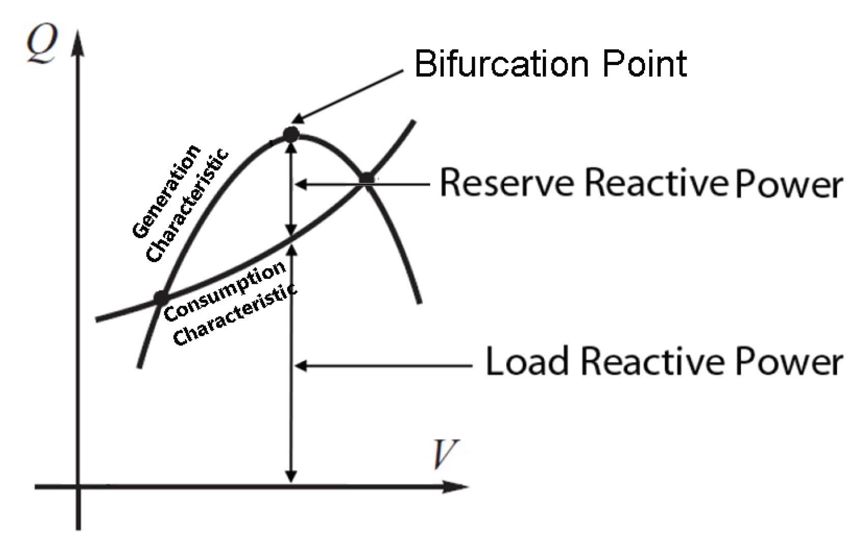
2.3.4. Reactive Reserve Support Index

The system’s voltage security depends on the availability of reactive power support in the area. The system’s reactive power generation with respect to variability of wind power was given in Equations (6) and (7). Accordingly, the Reactive Capability Index (RCI) is defined by:
R C I = Q a v a i l a b l e A r e a Q l o a d
where Q a v a i l a b l e A r e a and Q l o a d represent total available reactive power and total reactive power consumption in the system, respectively. Greater values of R C I measure higher reactive power available for voltage support and is an indicator of higher voltage security, while smaller values indicate the potential for reactive power deficit that might trigger an event leading to voltage collapse. Figure 2 illustrates the relationship between available reactive power and voltage security.
Accordingly, R C I could be rearranged by:
R R S I = Q l o a d Q r e s e r v e A r e a
where R R S I is the Reactive Reserve Support Index with values ranging from [ 0 , ) , where smaller values of the index (closer to zero) indicate higher availability of reactive power that is an indication of a greater voltage security margin. As the system begins to move towards the bifurcation point, this index tends to larger values and, eventually, tends to infinity as the system runs out of available reactive power.

2.3.5. Security Index

In the process of contingency analysis, contingency events are applied to the system one at a time. For each contingency event, to quantify the variability of the wind power plant, system variables such as line flows, voltages, generation data, etc. are collected with respect to increments of wind power throughout the full operational range of the offshore wind power plant with reasonable shift steps. Using system variables for each shift step, the four introduced indices can be computed. As a result, for m-shift steps of wind power and u contingency events, a security matrix can be formed by:
Ψ = Ψ 11 Ψ 1 k Ψ j 1 Ψ j k
for Ψ = V R I , P L I , T L L I , and R R S I , j = 1 , , m and k = 1 , , u . The V R I j k , P L I j k , T L L I j k and R S S I j k are the indices computed for j-th level of wind power throughout the full span of wind power variability with m steps of power increment and the k-th operating condition out of the u contingency events considered.
Then, for each index, a vector that quantifies the variability of wind power can be defined by:
Ψ k = j = 1 m Ψ j k k = 1 , , u
for Ψ = V R I P L I T L L I R R S I T . The final Security Index (SI), defined by a risk function for a k-th contingency event, S I k , can be defined by:
S I k = s 1 V R I k + s 2 P L I k + s 3 T L L I k + s 4 R R S I k
where s 1 , , s 4 are weighting factors and are chosen based on the planner’s preference and the grid topology. The range of values for this index depends on the values chosen for the weighting factors. Regardless, greater values of this index represent higher severity of the given operating condition or contingency event.

3. Case Study

This study considers the integration of 1000 MW of offshore wind power in Lake Erie into the FirstEnergy/PJM transmission system as a case study to verify the utility of the introduced methodology. This section describes the details of this case study and the computational implementation of this methodology.

3.1. FirstEnergy/PJM Power System

This study uses an accurate computer model of the FirstEnergy/PJM system. PJM is an independent market operator in the Midwestern United States and is part of the Eastern Interconnection. FirstEnergy is a regional utility company, based in Akron, Ohio, within a geographical sub-region of PJM and serves 6 million customers in Ohio, Pennsylvania, West Virginia, Virginia, Maryland, New Jersey, and New York.

3.2. Wind Power Integration Scenario Development

The estimated geographic distribution of available wind power over the surface of Lake Erie was provided by the NREL, and, based on these estimates, five candidate POIs were identified within the FirstEnergy transmission system including Ashtabula, Perry, Eastlake, Lake Shore, and Avon Lake. Accordingly, three scenarios for the integration of a total of 1000 MW of offshore wind generation at a variety of POIs were developed subject to compatibility with the extant grid infrastructure:
  • Interconnecting a total of 1000 MW of offshore wind generation at a single POI, referred to as EC01
  • Interconnecting a total of 1000 MW of offshore wind generation through five 200 MW POIs across the lake, referred to as EC02
  • Interconnecting a total of 1000 MW of offshore wind generation through two 500 MW POIs across the lake, referred to as EC03
Figure 3 shows the geographical location of the offshore wind power plant and the identified POIs.

3.3. Offshore Wind Power Plant Modeling

For computational purposes, the 1000 MW offshore wind power plant is modeled by an aggregated model that includes a synchronous generator connected to a P V bus through a 34.5 kV collector and export cables for the offshore system. The wind turbine model parameters used in this study are based on a Type 3 GE 3.6-MW offshore wind turbine with a variety of capability to provide reactive power support and the control strategy. Accordingly, the R 00 models correspond to a machine with no reactive support capability, the R 01 to a machine with limited reactive support capability (–7.5%/7.5%), and R 02 to a machine with full reactive support capability (–43.0%/+57.8%). The wind machines were set to cover a complete range of power generation by the offshore wind power plant from 0 MW to 1000 MW. The substation transformer is rated on the basis of the wind turbine generators and has a typical impedance of approximately 8% [26].
A static VAR compensator (SVC) with significant compensation capacity was incorporated at each POI to provide ancillary service (reactive power generated/consumed) as needed by the grid. The SVC is modeled as a controllable shunt device that allows for automatic voltage control during load flow simulations and is set to regulate voltage at the POI [26].

3.4. Generation Dispatch Scenarios and Load Assumptions

In this paper, summer 2015 load data from the Eastern Interconnection were used. The system model contains approximately 63,000 system buses, 9091 generators, with a total of 936,266 MW and 444,200 MVAr of installed generation capacity to serve the load of 685,469 MW and 201,005 MVar.

3.5. Contingency Events

FirstEnergy provided a contingency list that included generation units, transformers, line segments, complete lines, and synchronous condenser outages. These events were used to perform the contingency analysis.

3.6. Computer Implementation

The main objective of this case study is to understand the impacts of the integration of 1000 MW of offshore wind generation into the FirstEnergy/PJM system. The second objective is to assess the impacts of retirement or loss of one of the largest power plants in the area (Perry, with a capacity of 1200 MW and 625 MVAr) upon integration of the offshore wind power plant. According to these objectives, the computational implementation of this study was carried out using 36 cases that were developed for each of the interconnection scenarios (EC01, EC02, and EC03), for a total of 108 cases. These cases included three degrees of freedom for the reactive capability of the offshore wind machines (0 MVAr, –7.5%/+7.5% MVAr and –43.0%/+57.8% MVAr), three degrees of freedom for the point of voltage regulation (voltage regulation at the machine terminals, voltage regulation at the POI, and voltage regulation at the collector system), two degrees of freedom for the operation of the SVC (on and off), and two degrees of freedom for the operation of Perry (on and off). The description of these cases is shown in Table 1.

3.6.1. Normal Operation

For normal operation analysis, for each case, the wind generation was shifted across its 100% capacity with shift steps of 1%. Through every step change in wind generation, other non-wind generator units in the FirstEnergy area were redispatched to pick up missing generation of the wind power plant and a power flow calculation was done. For each power flow, system variables from all transmission lines, generation units, and substations in the FirstEnergy operating territory were recorded and merged. As a result, two main datasets were produced for each shift step:
  • The first dataset contains information about voltage magnitudes;
  • The second dataset contains information about power flows.
These datasets contain data that represent all possible voltage magnitude and power flow values for the system considering variable wind power.
In an ideal stable power system, voltage magnitudes across the system are regulated at 1.0 p.u. This is realized by voltage regulation data showing identical statistical measures of mode, mean, and median of 1, with an estimated density function that follows a normal distribution. As the voltage magnitudes across the system begin to deviate from 1.0 p.u. and spread out with a wider range, these statistical measures start to vary. As a result, the estimated density function begins to deviate from a normal distribution. Based on this notion, to analyze each dataset and process them to acquire meaningful information, the following statistical approach was used:
1.
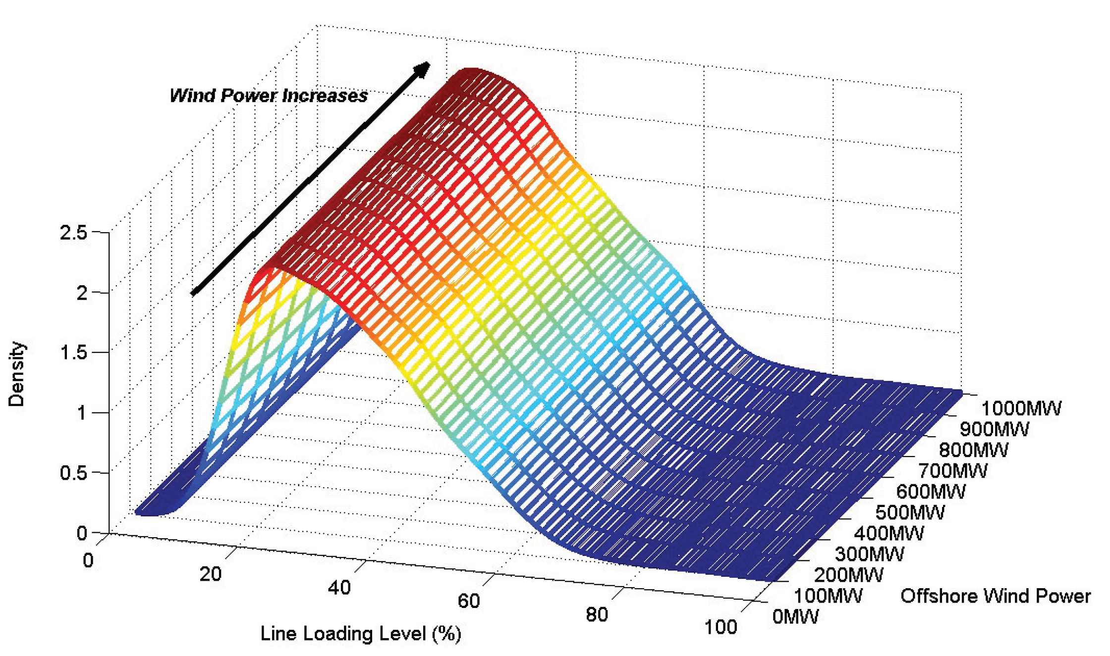
First, kernel density estimation (KDE) was applied to each of the datasets to estimate the density function of each dataset with an equal weight for all data points. The outcome of KDE shows how the variability of wind generation would impact voltage regulation and line loading conditions for each case.
2.
The next step was to calculate the dataset maximum, minimum, mode, mean, and median values for each case. These values provide a sufficient understanding of how the data points are distributed and how close to a normal distribution their distributions are.
  • Maximum and minimum measures indicate whether or not any voltage violation occurs, according to acceptable grid operating standards.
  • Mode measure shows the most frequently recorded voltage magnitude. The closer the mode value is to 1 is an indication of better system performance.
  • The last metric is the difference between mean and median. The smaller values for this measure indicate that the voltage data has a symmetric distribution similar to a normal distribution. Positive values for this difference show a trend to voltage rise across the system, whereas negative values indicate a trend to voltage drop across the system. This measure is similar to kurtosis and skewness in which the heaviness of the tail and shoulders of the distribution is used for interpretation. But it is easier to compute for datasets from power systems where the long tails of the probability distribution may not be a concern.
3.
The last step was to compare the distribution of datasets to a normal distribution. The outcome of this comparison provides information about the probability of any voltage or power flow value with respect to the wind variability.

3.6.2. Contingency Operation

For contingency operation analysis, for each case, the wind power was shifted across its capacity with shift steps of 10%. Similar to normal operation analysis, through every step change, non-wind generation was redispatched to meet the load demand and a power flow calculation was performed. For each power flow, the system variables from all transmission lines, generation units and substations in the FirstEnergy operating territory were recorded.
For each case and step shift of wind power, if power flow converged and intact operation was stable, then a series of contingency events were applied to the system, one outage event at a time. The outage list was provided by FirstEnergy and consisted of 64 contingency events that included generation, line segments, entire lines, and synchronous condenser outages. During each outage event, the system variables were recorded.
By using the proposed contingency ranking method, for each shift step for variable wind, the four indices, V R I j k , P L I j k , T L L I j k and R R S I j k , were computed (for the j-th level of wind power and the k-th contingency event). Then, S I k , the security index for the k-th event, was computed by first summing up the computed Ψ j k for all levels of wind power, as given in Equation (20), and then using the risk function, as given in Equation (21). In this study, the weighing factors for s 1 , , s 4 were assigned, equally, with the value 1. Finally, the contingency events were ranked in a descending order according to their security index to identify the most severe events for the offshore wind power plant integration.

4. Results and Discussion

This section presents the results and findings from all cases studied. First, results from analysis of normal operation are presented and then results from contingency ranking follow.

4.1. Normal Operation

During normal operation all of the generation units and lines are in operation without any contingency events. This section investigates how variability of the offshore wind power plant can affect voltage and thermal stability of the FirstEnergy/PJM transmission system and assesses whether or not the stability of the system is threatened as a result of the offshore wind power plant integration.

4.1.1. Voltage Stability

This section investigates the impacts of offshore wind generation on steady-state voltage stability. The FirstEnergy/PJM requires that 138 kV to 345 kV transmission and sub-transmission level apparatus operate within the ranges of 0.92–1.05 pu [27]. Figure 4a,b show the results for voltage regulation across the base case system (574 lines in total). These curves are the probability density estimates of simulated voltage data and compare their distribution to the normal distribution.
These plots show that no undervoltage condition has been recorded; however, two 138-kV lines are operating in a slightly overvoltage condition. In addition, 99.6% of the lines operate within the range of 0.977–1.035 p.u. The mean and mode values of the simulated voltage magnitudes are 1.002 p.u. and 1.013 p.u., respectively.
Figure 5 and Figure 6 illustrate how the density function of the voltage magnitude distribution changes with respect to the variability of the offshore wind power plant. They show that as power generation by the wind power plant increases, the distribution of voltage data becomes more symmetric and moves closer to a normal distribution. At 1000 MW offshore wind power generation, the voltage mode, median, and mean values are 1.014 p.u., 1.003 p.u., and 1.004 p.u., respectively. At 0 MW of offshore wind power generation, the mode value remains at 1.014 p.u., but the median and mean values move to 1.006 p.u. and 1.005 p.u., respectively. Clearly, the level of power generation by the offshore wind power plant has a direct impact on voltage regulation. Overall, across all levels of offshore wind power, no voltage violations occur.
Figure 7 illustrates the impact of the variability of wind power plant on the distribution of voltage datasets. This plot consists of a family of curves wherein each represents the voltage regulation across the system for a certain level of offshore wind generation. These curves compare the distribution of the voltage data points for varying level of wind generation to a normal distribution. These results suggest that after integration of the offshore wind power plant, for all levels of offshore wind power, the voltages are regulated within the standard range. In the base case, there are two data points within the overvoltage range and they are regulated properly upon operation of the offshore wind power plant. This is an indication of improved voltage stability.
Figure 5, Figure 6 and Figure 7 illustrate the results from the EC01 interconnection scenario. The results from EC02 and EC03 are similar and, therefore, are not shown.
Statistical measures of voltage data for all cases considered are compared in Figure 8, Figure 9, Figure 10 and Figure 11 show range, mode, and difference between median and mean of simulated voltage for all interconnections considered: EC01, EC02, and EC03.
Figure 8 shows the range of simulated voltage magnitudes across the system. The results here show that the integration of offshore wind into this transmission system improves voltage regulation for all levels of wind generation. In fact, the maximum recorded voltage in the base case (system without a wind power plant), shown by the red solid line, were regulated properly and moved closer to the operator’s standard range. This agrees with the findings from Figure 5, Figure 6 and Figure 7.
The second point to note is that there are no voltage violations for all EC01 and EC03 cases and the majority of the EC02 cases. For the EC02 interconnection scenario (5 POIs), in those cases that represent wind machines with either no or limited reactive support capability, voltage violations occurred (shown by the red dashed line). Figure 9 shows the distribution of the voltage data for the EC02 cases with a minimum of one voltage violation.
The results shown in Figure 9 outline that in those cases in which voltage violation occurred, the probability of the voltage violation is less than 4% for the full operational range of the offshore wind power plant. Overall, it can be concluded that the location of the POI and the capability of the wind machine to provide reactive power support are contributing factors in voltage regulation.
Figure 10 shows mode values for voltage data for all cases studied. It can be seen that the system remained stiff and well regulated upon the integration of the offshore wind power plant as the mode values did not change significantly.
Figure 11 shows the difference between mean and median values for voltage data for all cases studied. It can be seen that the symmetry of the voltage magnitudes in the EC01 and EC03 cases with Perry online remained approximately the same as in the base case. The EC01 cases with Perry offline showed a slight tendency toward voltage rise, whereas the EC03 cases with Perry offline showed a slight tendency toward voltage drop. However, neither of these two integration scenarios led the system to instability (there were no undervoltage violations). The EC02 cases with the SVC operated at the POI showed a distribution identical to that of the base case, whereas the EC02 cases with no SVC operating at the POI showed a tendency toward voltage rise. The contribution of the offshore wind power plant reactive capability and its voltage control scheme are not significant.
It is noticeable that the EC01 cases deliver the most robust performance in voltage regulation across this system for all levels of wind generation, with and without Perry. In all cases studied, no voltage anomaly was observed; thus, it is safe to conclude that the voltage data were nearly symmetrical and their distributions are very close to that of the base case.
One of the primary indicators for steady-state voltage instability is undervoltage violations at any given bus across the system as the operating point begins to approach the voltage collapse point. The results of the voltage analysis reveal that the FirstEnergy/PJM system does not experience this condition. In addition, in all cases studied, including the base case, the difference between mean and median was very small; therefore, for all levels of offshore wind generation, the system operates in stable region. It is safe to say that the integration of the offshore wind power plant in Lake Erie will not negatively affect the steady-state voltage stability of this transmission system. Additionally, the results from cases without Perry (cases 19 to 36 of EC01, EC02, and EC03) show that upon integration of 1000 MW wind power plant using all three studied interconnection scenarios, retirement or loss of Perry does not threaten voltage stability of the system.

4.1.2. Thermal Stability

This section discusses the impacts of offshore wind generation on loading condition of FirstEnergy/PJM transmission system and its steady-state thermal stability.
Figure 12 presents the base case results from the loading analysis of this transmission system. The results here indicate that almost 99.5% of the transmission lines in the base case were loaded below 80% of their nominal rating and more than 50% of them are loaded below 25% of their nominal rating. However, there is a 138-kV line operating in an overloaded condition, exceeding 3.1% of its nominal loading capacity.
Figure 13 and Figure 14 visualize the effect of wind power generation variability on loading of this transmission system. On these curves, it can be noticed that for higher levels of wind generation, the mode value moves to 23% from 21%. Nonetheless, there is a very small difference in the distribution of line loading data after the introduction of the wind power plant and for different levels of wind generation. This is because this system is very lightly loaded and therefore can easily accommodate the generated power from the wind power plant.
To investigate how different integration scenarios could impact loading of the lines, Figure 15 compares the distribution of system’s data for all cases studied. The results show that the distribution plots for all cases follow two main patterns and overlap to form two main plots. The factor that distinguishes the cases and their corresponding distribution is the operational status of Perry. As shown in this figure, in all cases, with and without Perry, there is a narrow probability of line overload; in cases with Perry online it is 0.002% with overload of up to 13% of the line’s nominal rating and in cases with Perry offline it is less than 0.001% with overload of up to 3% of the line’s nominal rating. The plots shown in Figure 15 are from EC01. The results from EC02 and EC03 are nearly identical and, thus, are not shown. It can be concluded that the location of the POIs does not have a significant impact on the overall loading of this system, however the operating status of Perry does.
In summary, the primary factor in the loading level of this transmission system is the operational status of Perry. The second factor is the level of power production by the offshore wind power plant. Other factors examined have no notable impact on the loading level of the system.
From the results shown in this section, it can be concluded that this transmission system is sufficient, in terms of capacity, to accommodate 1000 MW of offshore wind generation, as introduced in this study. Additionally, the retirement or loss of Perry does not threaten the transfer capability of this system upon integration of the wind power plant, for all three integration scenarios. Overall, thermal stability is a concern when the transmission lines operate in a heavily loaded condition; however, in this study, it was found that the FirstEnergy/PJM transmission system does not experience this operating condition.

4.2. Contingency Operation

This section describes the results from the steady-state contingency analysis using the proposed security index and outlines the findings. The main application of the proposed security index is to conduct contingency ranking and monitoring in power systems with variable generation units and to provide an assessment of how their variability effects the security of the system.
Figure 16a–c shows the security index for all cases and contingency events studied. Interestingly, the results intrinsically form two distinct surfaces and the decisive factor appears to be the operation of Perry. As a reminder, higher values of the security index indicate a lower security for the system. Having this in mind, in each of the figures, the upper surface represents the cases with Perry offline while the lower surface represents the cases with Perry online. Accordingly, these figures reveal that the loss of Perry has an adverse impact on the security of the system that includes the offshore wind farm. But it does not interrupt the power delivery in the system. Understandably, loss of a 1200 MW power plant adversely influences the security of the system. This shows the effectiveness of the contingency ranking method introduced in this paper.
This index can be used for contingency ranking as the S I contains the information necessary to identify the severe events. The greater the index, the more severe the contingency event, for all cases. Table 2 provides a list of the top 10 severe contingencies for six selected cases studied. For comparison purposes, the cases with and without Perry are also shown.
The results shown inTable 2 reveal a consistent ranking for the contingency events among all EC01, EC02 and EC03 cases. For instance, Events 24 and 40 are consistently ranked 1st or 2nd regardless of the interconnection scenario and operational status of Perry. However, ranking of event 17 significantly changes for the cases with and without Perry. The S I of this event for Case 1, EC01, is 1.240 placing it in the 8th position in the severity ranking while for Case 7, EC01, the S I is 1.446, ranking this event at 34th. In fact, this contingency represents loss of a 345 kV transmission line that is transmitting power directly from Perry. Hence, the offline status of Perry reduces its outage severity. This also verifies the utility and accuracy of the contingency ranking method introduced in this paper.
The results indicate that the EC01 interconnection provides the highest security during contingency operation. The S I values for the EC01 interconnection are the smallest among the three interconnection considered here. It is also noticeable that the S I values for cases in which Perry is offline, are significantly higher than the same cases in which Perry is online, demonstrating that the loss of Perry reduces the security of this system. This agrees with the finding evidenced in Figure 16a through Figure 16c.

5. Conclusions

This study present a statistical approach for the steady-state stability analysis of large-scale power systems and addresses normal and contingency operation. This method is practical for offshore wind integration planning studies and is easy and efficient to implement. The normal operation relies on statistical measures within the system’s recorded data and their distribution. The contingency analysis relies on a risk-based security index to identify the most severe contingency events and most secure interconnection scenario by considering variability of the offshore wind power plant.
This study focused on the investigation of steady-state operational impacts of integration of 1000 MW of offshore wind in the U.S. Great Lakes region. Specifically, this study focused on the FirstEnergy/PJM transmission system by considering its current configuration and operational status. In particular, operational issues including voltage regulation and power transfer capability were investigated. Feasible offshore wind integration scenarios were examined to identify vulnerability of the system. The 63k-bus U.S. Eastern Interconnection was used for the case study.
The results showed that the integration of offshore wind power plants could improve voltage stability across the system. The results also showed that in a lightly loaded power system, such as the FirstEnergy system studied in this paper, line congestion is not a concern when adding wind generation capacity. Additionally, in this particular case study, retirement or loss of Perry can negatively impact the steady-state stability of the system.
Although this study focused on integration of an offshore wind power plant, this methodology is applicable for integration of all types of variable generation units.

Author Contributions

The authors all equally contributed to this research. All authors have read and agreed to the published version of the manuscript.

Funding

This work was supported by the U.S. Department of Energy under Grant No. DE–EE0005367: Great Lakes Offshore Wind: Utility and Regional Integration Study. NREL’s contribution to this work was supported by the U.S. Department of Energy under Contract No. DE-AC36-08GO28308 with the National Renewable Energy Laboratory.

Acknowledgments

The authors thank S. Barnes and R. D’Aquila from GE and R. Kolacinski from Case Western Reserve University for their assistance. The U.S. Government retains and the publisher, by accepting the article for publication, acknowledges that the U.S. Government retains a nonexclusive, paid-up, irrevocable, worldwide license to publish or reproduce the published form of this work, or allow others to do so, for U.S. Government purposes.

Conflicts of Interest

The authors declare no conflict of interest.

References

  1. Machowski, J.; Bialek, J.; Bumby, J. Power System Dynamics: Stability and Control; John Wiley & Sons: Hoboken, NJ, USA, 2008. [Google Scholar]
  2. Sajadi, A.; Kolacinski, R.; Loparo, K. Impact of Wind Turbine Generator Type in Large-Scale Offshore Wind Farms on Voltage Regulation in Distribution Feeders. In Proceedings of the IEEE Power & Energy Society Innovative Smart Grid Technologies Conference (ISGT), Washington, DC, USA, 18–20 February 2015; pp. 1–5. [Google Scholar]
  3. Vittal, E.; O’Malley, M.; Keane, A. A Steady-State Voltage Stability Analysis of Power Systems with High Penetrations of Wind. IEEE Trans. Power Syst. 2010, 25, 433–442. [Google Scholar] [CrossRef]
  4. Baghsorkhi, S.S.; Hiskens, I.A. Impact of Wind Power Variability on Sub-Transmission Networks. In Proceedings of the IEEE Power and Energy Society General Meeting, San Diego, CA, USA, 22–26 July 2012; pp. 1–7. [Google Scholar]
  5. Li, H.; Haq, E.; Abdul-Rahman, K.; Wu, J.; Causgrove, P. On-line voltage security assessment and control. Int. Trans. Electr. Energy Syst. 2014, 24, 1618. [Google Scholar] [CrossRef]
  6. Ejebe, G.; Irisarri, G.; Mokhtari, S.; Obadina, O.; Ristanovic, P.; Tong, J. Methods for Contingency Screening and Ranking for Voltage Stability Analysis of Power Systems. In Proceedings of the IEEE Power Industry Computer Application Conference, Salt Lake City, UT, USA, 7–12 May 1995; pp. 249–255. [Google Scholar]
  7. Yokoyama, A.; Sekine, Y. A static voltage stability index based on multiple load flow solutions. In Proceedings of the Bulk Power System Voltage Phenomena-Voltage Stability and Security, Potosi, MO, USA, 19–24 September 1989. [Google Scholar]
  8. Chiang, H.-D.; Jumeau, R. Toward a practical performance index for predicting voltage collapse in electric power systems. IEEE Trans. Power Syst. 1995, 10, 584. [Google Scholar] [CrossRef]
  9. Foss, O.B.; Flatabo, N.; Hahavik, B.; Holen, A.T. Comparison of Methods for Calculation of Margins to Voltage Instability. In Proceedings of the Athens Power Tech, Joint International Power Conference (IEEE, 1993), Athens, Greece, 5–8 September 1993; Volume 1, pp. 216–221. [Google Scholar]
  10. Meliopoulos, A.S.; Cheng, C. A New Contingency Ranking Method. In Proceedings of the SoutheastCon, Honolulu, HI, USA, 1–4 April 1990; pp. 837–842. [Google Scholar]
  11. Subcommittee, P.M. IEEE reliability test system. IEEE Trans. Power Appar. Syst. 1979, 2047–2054. [Google Scholar] [CrossRef]
  12. Donde, V.; Lopez, V.; Lesieutre, B.; Pinar, A.; Yang, C.; Meza, J. Identification of Severe Multiple Contingencies in Electric Power Networks. In Proceedings of the IEEE 37th Annual North American Power Symposium, Manhattan, KS, USA, 22–24 September 2005; pp. 59–66. [Google Scholar]
  13. Brandwajn, V.; Kumar, A.; Ipakchi, A.; Bose, A.; Kuo, S.D. Severity indices for contingency screening in dynamic security assessment. IEEE Trans. Power Syst. 1997, 12, 1136. [Google Scholar] [CrossRef]
  14. Liu, H.; Bose, A.; Venkatasubramanian, V. A fast voltage security assessment method using adaptive bounding. IEEE Trans. Power Syst. 2000, 15, 1137. [Google Scholar]
  15. Limbu, T.R.; Saha, T.K.; McDonald, J.D. Comparing Effectiveness of Different Reliability Indices in Contingency Ranking and Indicating Voltage Stability. In Proceedings of the Australasian Universities Power Engineering Conference, (AUPEC2005), Hobart, Australia, 25–28 September 2005; pp. 568–573. [Google Scholar]
  16. Greene, S.; Dobson, I.; Alvarado, F.L. Sensitivity of the loading margin to voltage collapse with respect to arbitrary parameters. IEEE Trans. Power Syst. 1997, 12, 262. [Google Scholar] [CrossRef] [Green Version]
  17. Nims, J.W.; El-Keibb, A.; Smith, R. Contingency ranking for voltage stability using a genetic algorithm. Electr. Power Syst. Res. 1997, 43, 69. [Google Scholar] [CrossRef]
  18. Wan, H.; McCalley, J.D.; Vittal, V. Risk based voltage security assessment. IEEE Trans. Power Syst. 2000, 15, 1247. [Google Scholar] [CrossRef]
  19. Vijayan, P.; Sarkar, S.; Ajjarapu, V. A Steady-State Voltage Stability Analysis of Power Systems with High Penetrations of Wind. In Proceedings of the IEEE Power & Energy Society General Meeting, PES-09, Calgary, AB, Canada, 26–30 July 2009; pp. 1–8. [Google Scholar]
  20. Miller, N.; Shao, M.; Pajic, S.; D’Aquila, R. Eastern Frequency Response Study; GE-Power Systems Energy Consulting: Schenectady, NY, USA, 2013. [Google Scholar]
  21. Miller, N.W.; Price, W.W.; Sanchez-Gasca, J.J. Dynamic Modeling of GE 1.5 and 3.6 Wind Turbine-Generators; GE-Power Syst. Energy Consulting: Schenectady, NY, USA, 2003. [Google Scholar]
  22. ABB. Submarine Cable Systems: Attachment to XLPE Land Cable Systems-Users Guide; XLPE Submarine Cable Systems: Västerås, Sweden, 2010. [Google Scholar]
  23. Gutman, R. Application of line loadability concepts to operating studies. IEEE Trans. Power Syst. 1988, 3, 1426. [Google Scholar] [CrossRef]
  24. Savulescu, S.C. Real-Time Stability Assessment in Modern Power System Control Centers; John Wiley & Sons: Hoboken, NJ, USA, 2009; Volume 42. [Google Scholar]
  25. Schafer, K.; Verstege, J. Adaptive procedure for masking effect compensation in contingency selection algorithms. IEEE Trans. Power Syst. 1990, 5, 539. [Google Scholar] [CrossRef]
  26. Barnes, S. Progress Report—Great Lakes Offshore Wind: Utility and Regional Integration Study; General Electric (GE): Pittsburgh, PA, USA, 2014. [Google Scholar]
  27. Mackauer, J.; Syner, J.; Bowers, P.; Detweiler, J. FirstEnergy/PJM Requirements for Transmission Connected Facilities; FirstEnergy: Akron, OH, USA, 2013. [Google Scholar]
Figure 1. Voltage stability assessment in the presence of a wind power plant—adapted from [1].
Cleantechnol 02 00020 g001
Figure 2. Conceptual visualization of relationship between available reactive power and voltage security—adapted from [1].
Cleantechnol 02 00020 g002
Figure 3. Map of Interconnection Scenarios into the FirstEnergy System.
Cleantechnol 02 00020 g003
Figure 4. Distribution measures for the voltage regulation in the FirstEnergy transmission system—base case.
Cleantechnol 02 00020 g004
Figure 5. Wind power variability vs. probability density function of voltage regulation curve in FirstEnergy/PJM transmission system.
Cleantechnol 02 00020 g005
Figure 6. Impact of wind generation variability on voltage regulation in the FirstEnergy/PJM transmission system.
Cleantechnol 02 00020 g006
Figure 7. Wind power variability vs. distribution probability of voltage regulation curve in the FirstEnergy/PJM transmission system.
Cleantechnol 02 00020 g007
Figure 8. Voltage range in the FirstEnergy transmission system.
Cleantechnol 02 00020 g008
Figure 9. Distribution probability of voltage regulation curves in the FirstEnergy/PJM transmission system for the EC02 cases 1–9 with a voltage violation.
Cleantechnol 02 00020 g009
Figure 10. Voltage mode in FirstEnergy transmission system.
Cleantechnol 02 00020 g010
Figure 11. Difference between voltage mean and median in the FirstEnergy transmission system.
Cleantechnol 02 00020 g011
Figure 12. Distribution probability of line loading in the FirstEnergy/PJM transmission system—base case.
Cleantechnol 02 00020 g012
Figure 13. Wind power variability vs. probability density function of loading level in FirstEnergy/PJM transmission system.
Cleantechnol 02 00020 g013
Figure 14. Impact of wind power variability on loading level in the FirstEnergy/PJM transmission system.
Cleantechnol 02 00020 g014
Figure 15. Distribution probability of loading levels in the FirstEnergy/PJM transmission system.
Cleantechnol 02 00020 g015
Figure 16. Contingency ranking in the FirstEnergy transmission system.
Cleantechnol 02 00020 g016
Table 1. List of Studied Cases
Case No.Voltage ControlReactive CapabilitySVCPerry
1V00R00OFFON
2V01
3V02
4V00R01
5V01
6V02
7V00R02
8V01
9V02
10V00R00ON
11V01
12V02
13V00R01
14V01
15V02
16V00R02
17V01
18V02
19V00R00OFFOFF
20V01
21V02
22V00R01
23V01
24V02
25V00R02
26V01
27V02
28V00R00ON
29V01
30V02
31V00R01
32V01
33V02
34V00R02
35V01
36V02
R00: (0 MVAr), R01: (–7.5%/+7.5% MVAr), R02: (–43.0%/+57.8% MVAr); V00: Voltage regulation at the terminals of machines; V01: Voltage regulation at the POI; V02: Voltage regulation at the collector system.
Table 2. List of Top 10 Most Severe Contingency Events and Their Ranking for Selected Cases.
Case 1, EC01Case 7, EC01Case 1, EC02Case 7, EC02Case 1, EC03Case 7, EC03
EventRankSIRankSIRankSIRankSIRankSIRankSI
4011.28021.53011.28721.56411.36211.593
2431.27611.54421.28511.57621.34821.582
3941.24761.48851.25561.52151.32271.534
1851.24731.52141.25831.56141.32331.574
4161.24471.48671.24891.50561.31981.528
3071.24381.48461.25171.51671.31191.522
1781.240341.446121.241431.470101.300401.480
991.236251.451131.237421.471171.296441.479
22101.23491.47991.23781.51281.304101.522
62111.232141.46081.243131.492151.297231.490

