
The Wisdom of the Data: Getting the Most Out of Univariate Time Series Forecasting


1
School of Management, University of Bath, Bath BA2 7AY, UK
2
Forecasting and Strategy Unit, School of Electrical and Computer Engineering, National Technical University of Athens, 15780 Athens, Greece
*
Author to whom correspondence should be addressed.
Forecasting 2021, 3(3), 478-497; https://0-doi-org.brum.beds.ac.uk/10.3390/forecast3030029
Submission received: 17 May 2021
/
Revised: 11 June 2021
/
Accepted: 21 June 2021
/
Published: 23 June 2021
(This article belongs to the Special Issue Feature Papers of Forecasting 2021)
Abstract
:Forecasting is a challenging task that typically requires making assumptions about the observed data but also the future conditions. Inevitably, any forecasting process will result in some degree of inaccuracy. The forecasting performance will further deteriorate as the uncertainty increases. In this article, we focus on univariate time series forecasting and we review five approaches that one can use to enhance the performance of standard extrapolation methods. Much has been written about the “wisdom of the crowds” and how collective opinions will outperform individual ones. We present the concept of the “wisdom of the data” and how data manipulation can result in information extraction which, in turn, translates to improved forecast accuracy by aggregating (combining) forecasts computed on different perspectives of the same data. We describe and discuss approaches that are based on the manipulation of local curvatures (theta method), temporal aggregation, bootstrapping, sub-seasonal and incomplete time series. We compare these approaches with regards to how they extract information from the data, their computational cost, and their performance.
Keywords:
information; combination; uncertainty; theta; temporal aggregation; bagging; sub-seasonal series1. Introduction
Univariate time series forecasting is the creation of extrapolations for a single variable based on past, time-ordered observations of the same variable. Despite the geometric increase in data availability, univariate forecasts are even today the basis for the decision making in many organisations. Improvements in the performance of such forecasts are crucial for reducing costs associated with operational, tactical, and strategic planning [1].
Nowadays, automatic time series forecasting can be easily achieved using dedicated forecasting software or open source packages. Examples include ForecastPro®, SAS Forecasting Server®, and the forecast package for R statistical software. Such software and packages offer tools for batch and automatic forecasting with minimal to zero manual input. They integrate families of models, like exponential smoothing [2] and autoregressive integrated moving average, ARIMA [3], that can capture a wide range of data patterns and produce extrapolations with ease. However, such families of models rely on assumptions that are barely met in practice, and struggle to select the most appropriate model for a given time series due to the uncertainties involved: identifying the optimal model form, estimating the optimal set of parameters, and dealing with the inherent uncertainty in the data [4].
The purpose of this article is to provide an overview of approaches that can be used to enhance the performance of univariate forecasting methods. There are four common characteristics that govern the approaches covered in this article. First, all approaches attempt to distil as much information from the original time series data as possible by exploring them through alternative lenses. This is achieved through amplification of specific time series features and transformation of the original time series. Second, the approaches build on the success of forecast combinations to offer improved forecasting performance while tackling uncertainties regarding model form and parameter specification. Third, all approaches are model-free in the sense that do not rely on a particular family or pool of models. Four, each of the approaches manage to handle at least one of the uncertainties associated with fitting forecasting models: model form, parameter, and data.
In summary, we consider, present, and discuss the following five approaches:
- Forecasting with sub-seasonal series (FOSS), in which a seasonal time series is split into multiple new series where only particular seasons (or sets of seasons) are observed and modelled [17];
We should clarify that although the literature involves several other univariate approaches in addition to the aforementioned ones for extracting more information from the original data and mitigating the drawbacks that forecasts from single forecasting methods may involve, these are not considered in the present study as they are not characterised by the four key attributes discussed earlier. For instance, when the forecast errors of a method display strong auto-correlations (e.g., because the method fails to fully capture seasonality or trend), a common approach is to adjust the forecasts originally produced according to their expected error, specified using a second univariate forecasting method on the residuals of the first one. TBATS [20] exponential smoothing state space model with Box-Cox transformation, ARMA errors, Trend and Seasonal components, and Theta with ARMA errors [21], are just some examples of this approach which, although enhances forecasting performance, does not rely on combinations. Similarly, decomposition techniques that allow for complex, multiple seasonal patterns to be captured [22], can be regarded as “wisdom of the data” approaches, but do not involve combinations, depending also on particular models and, in many cases, explanatory variables.
The next five sections expand on each of the above approaches: We offer a summary of the related research studies, we describe how these approaches handle and manipulate the original time series data, and we discuss the advantages gained from their application. Section 7 offers a cross-comparison of the approaches, with an emphasis on the uncertainties that each handles, as well as their computational cost. Finally, Section 8 offers our conclusions and insights for future research.
2. Theta Method
The theta method was the top-performing submission in the M3 forecasting competition [23]. Its name originates from the first letter of the Greek word for “temperature”, . Similarly to how a decrease or increase in the temperature would result in contraction or expansion, the theta method amplifies or smooths the local curvatures of a time series, i.e., the distances between the points of the series with those of a simple linear regression line, computed over its observations against time. The result of this local-curvatures manipulation process is the creation of new series that are called “theta lines”. The degree of amplification or reduction in the local variations is controlled by a parameter, , where a value of 1 corresponds to the original data with the original local curvatures. If , then the local variations are amplified; if , then the resulting theta line is smoother than the original data.
In its simplest form, the theta method decomposes the original data into two theta lines with parameters and [5]. The theta line with corresponds to linear regression on a time-trend indicator. This is a straight line that captures the long term trend of the data and has no local variations. The theta line with displays double the curvatures of the data. It is argued that this second theta line is able to better capture the short term variations in the data. Each of these two theta lines are extrapolated separately. Assimakopoulos and Nikolopoulos [5] used the forecasts of the linear regression on trend to extrapolate theta line with and the simple exponential smoothing (SES) method to produce forecasts for the other theta line (). Once the forecasts from the two theta lines have been produced, then these are combined with equal weights to form the forecast for theta line with that corresponds to the data with the original curvatures.
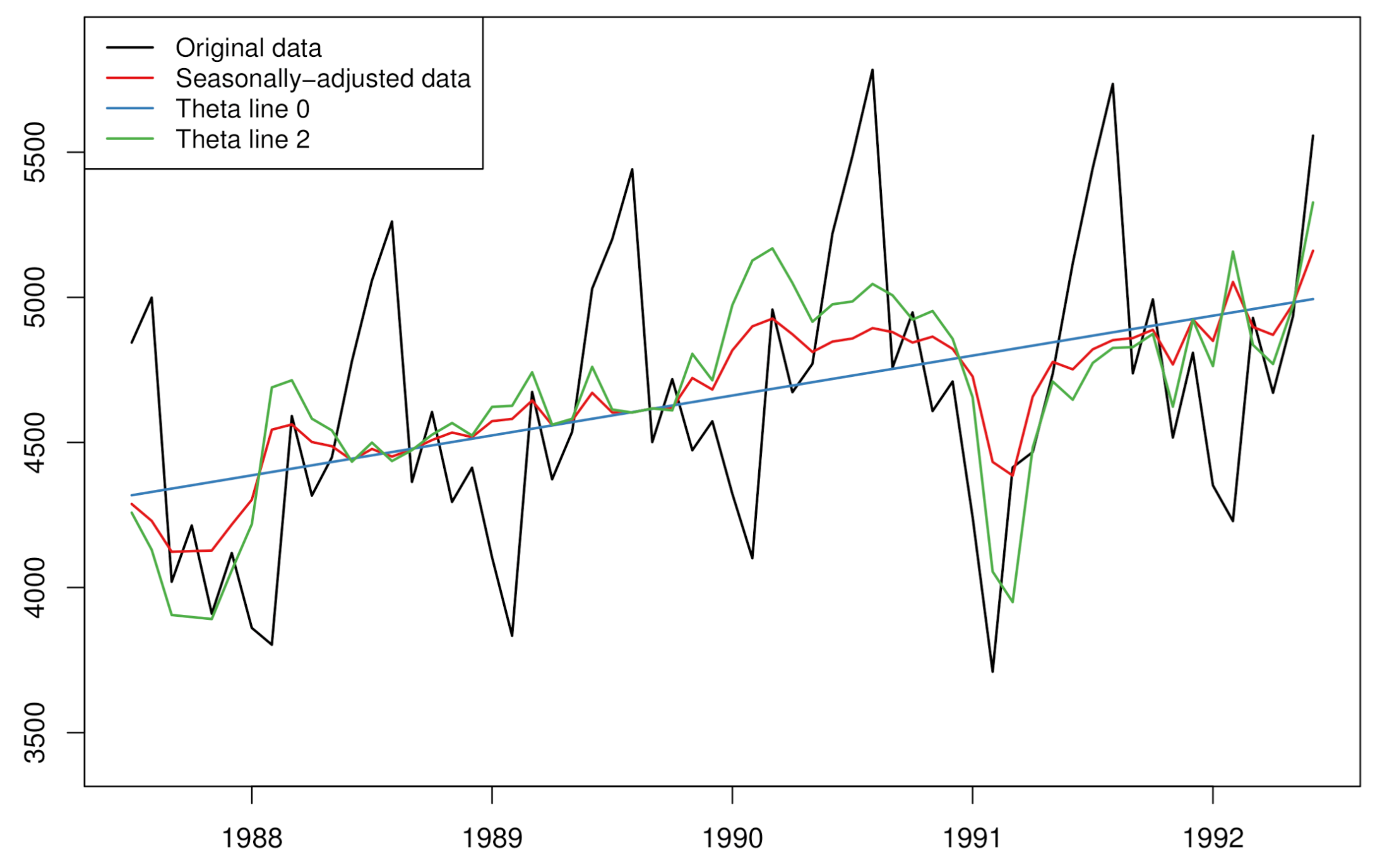
The above process works directly on data that do not exhibit seasonality. However, if the original data are seasonal, then they need to be adjusted for seasonality before the application of the theta decomposition. Assimakopoulos and Nikolopoulos [5] proposed the use of the classical decomposition method with the assumption that the seasonal pattern is multiplicative in nature; a not unreasonable assumption for real life applications. As an alternative, Spiliotis et al. [9] proposed using shrinkage estimators of time series seasonal indices to avoid cases where their values are exaggerated. In both cases, a simple statistical test based on the autocorrelation coefficient with a lag that matches the periodicity of the data is used to decide on the existence of a (sufficiently strong) seasonal pattern, typically considering a confidence level of 90%. This test is described in detail in [8]. If the theta decomposition is applied on the seasonally adjusted data, then the resulting forecasts are not seasonal, and a seasonal re-adjustment is needed. This is simply done by multiplying the combined forecasts with the respective seasonal indices computed earlier by the decomposition method. A visual example of producing theta lines from seasonal time series data is presented in Figure 1.
When theta is restricted to the simple form of two theta lines (0 and 2) that are extrapolated by the linear regression line and SES, then its application on some seasonally adjusted data is mathematically equivalent to SES with drift [6]. However, it would be more appropriate if theta is seen as a decomposition framework rather than a forecasting method. One can decide on the number of theta lines, their theta parameters, the forecasting methods to be applied on each of them, and the combination weights, among other modelling choices. In fact, as explained by Spiliotis et al. [9], “the advantage of theta derives exactly from (its) “divide and conquer” property: There is no single forecasting model capable of effectively capturing all possible time series patterns. Yet, if the series is decomposed into multiple lines of a reduced amount of information, improvements in forecasting accuracy are possible even for the case of conventional models”.
Several studies have worked on expanding the theta method to the aforementioned directions. Petropoulos and Nikolopoulos [24] examine the use of equal and unequal weights for the combinations of the two theta lines forecasts, and conclude that optimally choosing the combination weights per series may result in performance benefits. Petropoulos [25] proposes the addition of a third theta line with that is extrapolated by the damped-trend exponential smoothing method. He also suggests the addition of a second short term trend-line that is fitted on the most recent observations, which is closely connected with the concept of multiple starting points (see Section 6). Fioruci et al. [26] and Fiorucci et al. [8] offer generalised rolling origin evaluation methods and state space models for optimising the theta parameter of the second theta line, showcasing the benefits in the out-of-sample accuracy of the method. Thomakos and Nikolopoulos [27] expand the application of the theta method in a multivariate setting and show the conditions under which this is expected to work better than its standard, univariate implementation.
Two recent extensions on the theta method are particularly interesting. Following the work of Spiliotis et al. [9], Spiliotis et al. [10] offer a taxonomy of theta models that can capture several forecasting profiles regarding the type of trend (additive or multiplicative) and seasonality (none, additive, or multiplicative). This is a significance advancement since the original theta method was designed on the assumptions of a linear trend and multiplicative seasonality. The authors propose non-linear trends, but also alternative seasonal profiles in a framework that resembles that of the exponential smoothing family of models [6]. Moreover, they define a process for selecting an optimal theta method and offer a simple way to empirically estimate the prediction intervals. Their “AutoTheta” method shows improved performance over the standard theta method for both point forecast accuracy but also the estimation of uncertainty. Legaki and Koutsouri [28] deal with non-linear trends in an alternative fashion. They apply a Box-Cox transformation on the seasonally adjusted data prior to the theta decomposition and extrapolation. The value of the Box-Cox transformation parameter, , is selected so that the profile log-likelihood of a linear model fitted to the seasonally adjusted series is maximised, with the choice of being restricted in . A Box-Cox transformation allows the application of theta on data with non-linear trends but also results in stabilisation of the variance. The “Box-Cox Theta” was one of the solutions submitted in the M4 forecasting competition [29], resulting in very good point forecast accuracy with very low computational cost [30].
The theta method has performed well in a variety of settings that involve financial [31], tourism [32], and inventory forecasting [33]. It is not a surprise that nowadays it is considered to be one of the default time series forecasting benchmarks along with the automatic implementations of exponential smoothing and ARIMA [34], as showcased by the M4 forecasting competition [29]. The theta method is attractive for its simplicity, robust performance, and computational efficiency. The book of Nikolopoulos and Thomakos [35] exclusively focuses on the theory and applications of the theta method, highlighting the conditions under which it will outperform other forecasting methods. Several open source implementations of the theta method exist. We would like to spotlight the forecTheta package for R statistical software, as well as the functions thetaf() and theta() of the packages forecast and tsutils, respectively. Finally, Petropoulos and Nikolopoulos [36] offer a step-by-step tutorial of the standard theta method coupled with an implementation in just 10 lines of R code.
3. Multiple Temporal Aggregation
The theta method extracts more information from the data by amplifying or deflating the local curvatures. In other words, the theta method manipulates the data on the vertical axis of a standard time series plot. The next approach we explore manipulates the data on the horizontal axis, i.e., the time. Temporal aggregation refers to a time series transformation where a higher frequency series is translated into a series of lower frequency see Section 2.9.2 in [37]. For example, a time series on the daily frequency can be converted into a weekly-frequency series when considering non-overlapping time buckets of 7 days each. Different levels of temporal aggregation result in new, shorter series where the high frequency components (seasonality and noise) are filtered out while level and trends are made easier to discern and model. Moreover, when temporal aggregation is applied on very granular, intermittent data, then we observe a decrease on the degree of intermittence, i.e., the number of zero observations included in the series, thus facilitating the overall forecasting process. An example of the temporal aggregation process applied on fast moving data is presented in Figure 2.
Although it is possible that one focuses on modelling a single aggregation level, even if this is not the original level on which the data are recorded [38,39,40], more benefits will usually arise from modelling multiple temporal aggregation (MTA) levels and combining the resulting forecasts. Kourentzes et al. [11] offer one of the first systematic studies to explore the beneficial effects of MTA. Focusing on exponential smoothing models [2], they propose that model selection should be applied on each temporally aggregated series separately. The exponential smoothing model components (level, trend, and seasonality) are estimated per aggregation level and their additive-transformed estimates are averaged across levels. The summation of the three average components is the final forecast. This approach is known as the “multiple aggregation prediction algorithm” (MAPA). The need for averaging at a component level rather than at a forecast level was driven by the fact that seasonality may not be possible to estimate in some levels (consider, for instance, monthly data and an aggregation level of five periods). Combining at a component level avoids the excessive shrinkage of the seasonal pattern [41,42]. MAPA showcased improved performance over the exponential smoothing benchmark that was applied on the original data only [11]. The improvements of MAPA over the benchmarks were more obvious on the longer forecasting horizons.
MAPA, as introduced by Kourentzes et al. [11] and implemented with exponential smoothing, is a great solution for amplifying and smoothing data patterns for fast moving series. However, when the series become intermittent, with the presence of many zeros among the non-zero demand observations, then the toolbox of forecasting models applied across the various aggregation levels can be updated to include specialised methods for intermittent demands. Such methods include the Croston’s method [43] and the Syntetos-Boylan approximation (SBA) [44]. Petropoulos and Kourentzes [13] suggest the use of multiple temporal aggregation levels for the case of slow-moving demand series, where a selection between the Croston’s method and the SBA is made based on the degree of intermittence and the variability of the non-zero values [45]. Finally, if the average inter-demand interval becomes equal to unity (i.e., the intermittent data are sufficiently temporally aggregated to become non-intermittent), then Petropoulos and Kourentzes [13] suggest replacing specialised methods for intermittent demand with SES. The empirical results from the application of the MAPA version for intermittent demand data showed superior forecasting performance on a variety of metrics that included proxies for the inventory performance.
Another extension to MAPA was introduced by Kourentzes and Petropoulos [46] to allow the algorithm handle exogenous variables which are estimated as additional components. The concept is similar to how exponential smoothing models (ETS) are extended to include exogenous variables (ETSx). However, the multivariate version of MAPA (MAPAx) performs temporal transformation on the exogenous variables too. This, by turn, tackles the uncertainty associated with estimating not only the effects of such predictors, but also their timing, i.e., leading and lagging effects. Applied on demand volumes affected by promotions, MAPAx offered a performance that was better to either ETSx or ARIMAx (ARIMA models with exogenous variables), both in terms of accuracy and bias, across multiple planning horizons.
One of the most important milestones in the development of MTA has been its conceptualisation in a hierarchical fashion. This enabled to directly apply the advances of the rich hierarchical literature [47,48,49,50] to the MTA application, that includes the estimation of coherent forecasts from the base forecasts of each hierarchical node. In essence, each hierarchy consists of observations at the most granular frequency at the bottom level, which are then added up to higher hierarchical levels, with the top level usually being a full periodic cycle. For example, monthly observations are added to bi-monthly, quarterly, four-monthly, semesterly, and yearly. Temporal hierarchies were first proposed by Athanasopoulos et al. [14], who showed that such structures allow MTA to be applied to a wide range of forecasts that are not limited to exponential smoothing ones and could even include judgment. The authors performed a large simulation study to better understand why temporal hierarchies work better than simply modelling the original data. Finally, they discussed the managerial implications of MTA through a case study of accident and emergency demand data.
Since the work of Athanasopoulos et al. [14], there has been a spark of research studies around forecasting with temporal hierarchies (THIEF). We now provide some highlights. Spiliotis et al. [41] proposed three simple ways to improve performance of temporal hierarchies: (i) model combinations to the base forecasts prior reconciliation, (ii) additive and multiplicative bias adjustments to the base forecasts, and (iii) a selective application of temporal hierarchies so that unnecessary seasonal shrinkage is avoided for the time series that exhibit strong seasonality, closely related also to the work of Kourentzes et al. [51] on optimal selection of temporal aggregation levels. Jeon et al. [52] expanded temporal hierarchical forecasting from point forecast reconciliation to probabilistic coherent forecasts, showcasing its benefits on high frequency wind power production and electricity load data. Additionally, focusing on short term electricity load data, Nystrup et al. [53] showed that temporal hierarchical forecasting can be significantly improved when auto- and cross-correlations are taken into account in the reconciliation stage of the base forecasts. Finally, Kourentzes and Athanasopoulos [54] applied temporal hierarchies on intermittent demand data, arguing that some data patterns (trend and seasonality) are difficult to discern on low levels of aggregation where the degree of intermittence is high. They selectively used Teunter-Syntetos-Babai (TSB) [55] method for intermittent demand or ETS based on an intermittence threshold, which acts as a hyperparameter. Generally, the accuracy improvements were higher for lower intermittence thresholds, i.e., TSB switches to ETS when the intermittence is low, as investigated on 5000 time series depicting the demand of aerospace spare parts.
A fertile field for research is the integration of temporal aggregation forecasting with the more traditional cross-sectional one, towards what is dubbed as “cross-temporal forecasting”. To the best of our knowledge, Spiliotis et al. [42] were the first to investigate this issue, focusing on hourly electricity consumption data from a bank, disaggregated into branches and further disaggregated into energy uses. They proposed a sequential process where a simplified version of MAPA is first applied on the seasonally adjusted data, followed by reseasonalisation of the temporally combined forecasts and consequent application of cross-sectional hierarchical forecasting for the production of coherent forecasts across all cross-sectional levels. Kourentzes and Athanasopoulos [56] approached cross-temporal aggregation from a hierarchical approach, instead of using MAPA. Although they defined full cross-sectional hierarchies, they still used a sequential approach where they first apply temporal hierarchies for each cross-sectional node followed by cross-sectional reconciliation at each aggregation level with the resulting forecast being combined using equal weights towards a “consensus reconciliation matrix”. The authors showed that this approach resulted in improvements when applied on Australian tourism data. Yagli et al. [57] explored further the sequential implementation of cross-temporal hierarchies by comparing the appropriate order of application, i.e., spatial then temporal, or temporal then spatial. Using photovoltaic power generation data, they showed greater benefits when temporal aggregation is applied prior to cross-sectional (spatial), while they also provided evidence that temporal aggregation may not be needed at all levels of the cross-sectional hierarchy.
Overall, we can see a large number of studies over the last few years that focus on issues surrounding MTA. MTA is attractive as it offers significant performance improvements that are coupled with aligned decision making [14]. Forecasts are produced at different frequencies and are then reconciled, rendering them suitable for use in several functions within companies and organisations, including operational, tactical, and strategic planning. Although, normally, different teams and departments within organisations would produce their own sets of forecasts, MTA brings us one step closer to the concept of “one number forecast”, where the same sets of forecasts can be used for logistics, manufacturing, scheduling, budgeting, etc. Various implementations of MTA are available in open source forecasting packages that include the mapa() function of the MAPA package (MAPA and MAPAx), the imapa() function of the tsintermittent package (MAPA for intermittent demand data), and the thief() function of the thief package (temporal hierarchies) for R statistical software.
4. Bagging
The next approach that we investigate is called “bagging”, which is short for “bootstrapping and aggregation”. In brief, bagging is based on the resampling of the random component of a series towards the creation of new series with the same underlying patterns (trend and seasonality) but different remainder. Multiple forecasts are produced using the original and the bootstrapped series which are then aggregated (combined) to form the final forecast. In more detail, the steps for the bagging approach are as follows:
- A Box-Cox transformation is applied on the original series. The parameter for the Box-Cox transformation is automatically selected based on the Guerrero’s method [58], but other methods such as the maximisation of the profile log likelihood of a linear model fitted to the original data could be used. The purpose of this step is twofold. First, the variance of the series is stabilised. Second, multiplicative patterns are converted into additive ones;
- The Box-Cox transformed series is decomposed into its components. If the series has periodicity greater than unity (e.g., quarterly or monthly data), then the seasonal and trend decomposition using Loess STL [59] decomposition is applied to separate the transformed series into the trend, seasonal, and remainder components. If the series has no periodicity (e.g., yearly data), then a Loess decomposition is applied to separate the series into two components: trend and remainder;
- The remainder component of the above decomposition is bootstrapped towards the creation of new vectors of remainders that follow the empirical distribution of the original remainder vector;
- The bootstrapped remainder vectors are added to the other extracted components from the decomposition of step 2 (trend and, where applicable, seasonality) to form new bootstrapped series. These series have the same underlying structural patterns with the original series;
- An inverse Box-Cox transformation is applied on each of the bootstrapped series, using the same parameter of step 1. This transformation brings the bootstrapped series back to the same scale as the original data. Figure 3 shows the estimated bootstrapped series based on the original (seasonal) data;
- The original and the bootstrapped series are extrapolated using an automatic forecasting process, which may result on the use of the same or different model forms and parameters. In any case, many sets of forecasts are produced at the end of this step;
- The forecasts from the original and bootstrapped series of the previous step are aggregated (averaged).
Effectively, bagging should be seen as a data augmentation (or oversampling) approach applied in univariate settings, in the sense that the amount of modified series added over the existing one for training the forecasting methods and producing the final forecasts are solely based on the series being predicted. This is a key difference compared to the multivariate data augmentation approaches used in the literature for successfully implementing “cross-learning” (or “global”) forecasting methods [60], where the synthetic data share the underlying patterns of multiple series found in a broad set of series.
Bagging was first proposed by Bergmeir et al. [15], who applied it to improve the performance of exponential smoothing. They used the moving block bootstrapping MBB [61] algorithm to produce bootstrapped vectors of the remainder, and produced 99 bootstrapped series. The best ETS model was fitted on each of the original series and the 99 bootstrapped series in order to produce point forecasts. The final forecasts were obtained using the median operator, while the authors discuss that they also tried mean and trimmed means. Bagging on ETS offered improved performance over ETS simply applied on the original data. The authors also tried replacing Box-Cox and Loess decomposition with decomposition based on the components of the best ETS model fitted on the original data. The authors also explored replacing MBB with the sieve bootstrap method [62]. However, both these modifications resulted in, overall, inferior results.
In a follow-up study, Petropoulos et al. [4] sailed to explore the reasons behind the good performance of the bagging approach. They argued that bagging succeeds in tackling, at the same time, three sources of forecast uncertainty: (i) the uncertainty in selecting the correct model form, (ii) the uncertainty in estimating the model’s parameters, and (iii) the inherent uncertainty of the data. They devised three simple experiments to disintegrate the benefits of bagging:
- After producing the bootstrapped series the usual way, the authors identified the optimal models on these bootstrapped series. Instead of using the forecasts from these models directly, their model forms were applied back to the original data, for which a different optimal model form may have been identified. Effectively, the bootstrapped series provided the frequencies with which each model form was identified as ‘optimal’, and these frequencies were then translated into combination weights for averaging the point forecasts of the different model forms when applied on the original data. All model parameters and forecasts were estimated using the original data only. This variation of bagging is known as “bootstrap model combination” (BMC) and handles only the uncertainty in the model form;
- The optimal model form was identified using the original data only. Subsequently, this optimal model form was applied on the original data and the bootstraps to obtain multiple independent estimates of the model parameters. The combination of each set of model parameters with the unique optimal model form was then applied again on the original data to produce multiple sets of point forecasts. As with bootstrap model combination, the bootstrapped series were not used to produce forecasts directly. This variation solely handles the uncertainty in estimating the model parameters;
- The optimal model form and set of parameters were estimated using the original series only. Subsequently, this unique model form and set of parameters were applied on all bootstrapped series to produce multiple sets of point forecasts. This variation solely tackles the uncertainty associated with the data, as the bootstrapped series are not used for selecting between models or estimating their parameters.
Using the data from M and M3 forecasting competitions, the results of Petropoulos et al. [4] showed that, on average, tackling model uncertainty alone through bootstrap model combination offers benefits that are higher than bagging itself. Simply addressing the uncertainty in estimating the parameters of the applied model is overall worse than either bagging or bootstrap model combination but still slightly better than forecasting without bootstraps. Tackling only the data uncertainty does not offer notable gains. The authors went one step further towards generalising bagging by considering replacing the estimator (ETS) with ARIMA. The results were consistent, with bootstrap model combination being the best approach overall. Finally, they replaced MBB with two other bootstrapping approaches, circular block bootstrap CBB [63] and linear process bootstrap LPB [64], showing that the relative average ranks of the various approaches would not significantly change.
Although the last two studies focused on the performance of bagging when applied on families of models (ETS and ARIMA), bagging can also lead in improvements in the forecasting performance when applied on single methods. Dantas et al. [65] showed that bagging with the Holt-Winters method, an exponential smoothing method that is able to capture the trend and the seasonality in the data, results in better performance than either ETS, ARIMA, or bagged ETS when forecasting the demand for air transportation.
To control the effect of the covariance on the combination step of the bagging approach, Dantas and Cyrino Oliveira [16] proposed the use of clusters of similar forecasts. Instead of aggregating across all forecasts, a diverse set of forecasts are selected from each cluster and then these selected forecasts are combined across clusters. This simple trick leads to reduced variance of the forecasts and, as a result, in reduced forecast error. They tested their cluster-modified bagging approach using ETS and data from the M3 forecasting competition and showed improvements in the point forecast accuracy.
Meira et al. [66] extended the previous works towards allowing the various bagging approaches to produce robust prediction intervals. They proposed “treating and pruning” strategies to selectively exclude models from the pool of candidate models such that models with explosive or outlying prediction interval values are not considered. This not only improved the performance of bagging and its variations, but also offered improvements upon the standard ETS. Overall, the authors demonstrated that bootstrap model combination offered very competitive performance compared to other bagging variations, both in terms of point forecast accuracy but also uncertainty estimation.
Research around bagging is much more scarce compared to theta or MTA. However, it is a robust alternative to deal with the various sources of uncertainty; arguably, though, an expensive one. Most published studies use between 50 and 100 bootstraps per series, with the computational cost need to fit all models and produce forecast being increased with the same rate. Open source implementations of the bagging approach include the functions baggedETS() and baggedClusterETS() of the R packages forecast and tshacks, respectively.
5. Sub-Seasonal Series
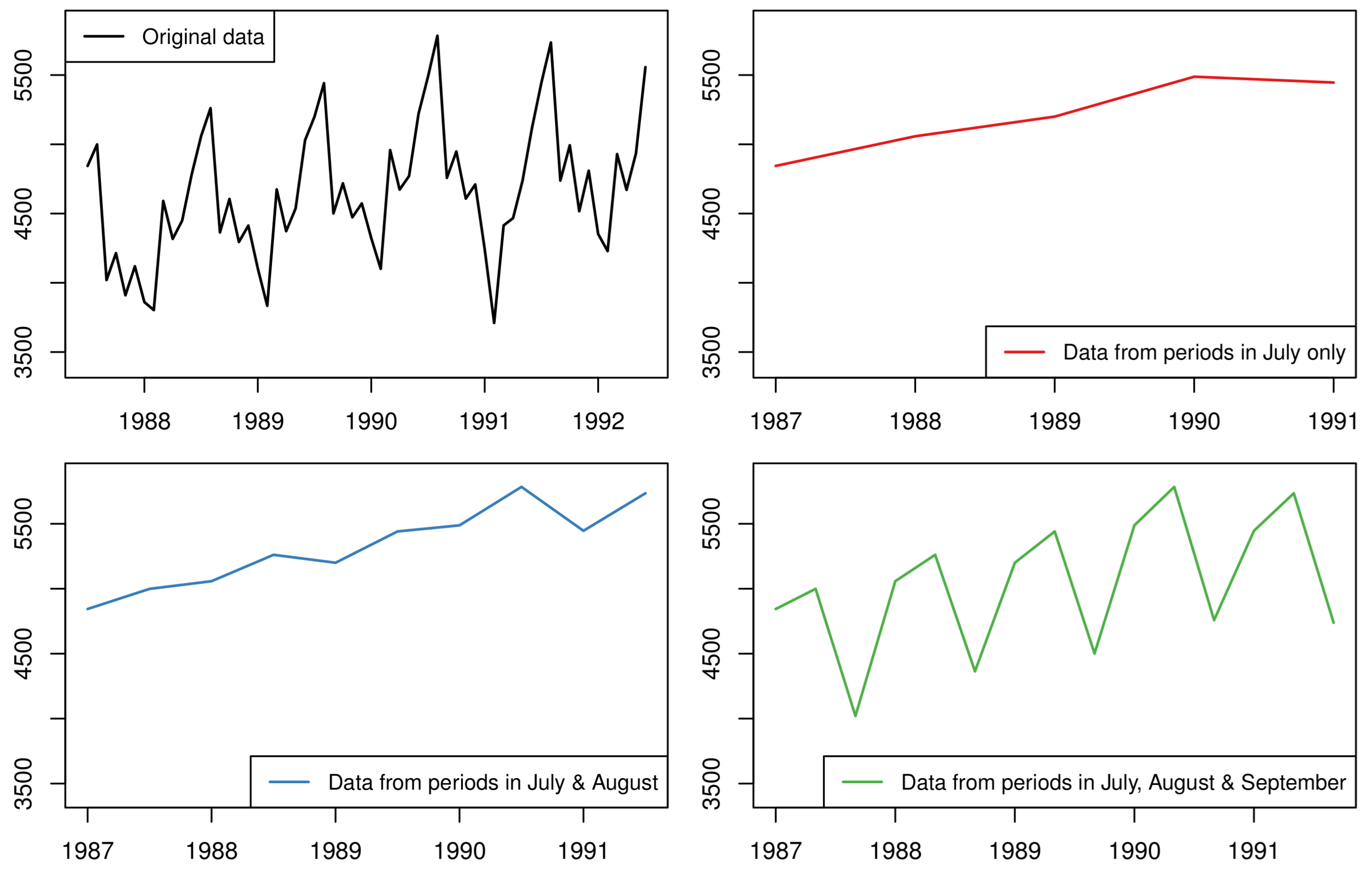
Instead of transforming a series to another of lower frequency through temporal aggregation using all observations, the next approach we review applies sub-sampling such that the resulting series includes only some of the periods within a periodic cycle. Consider, for instance, the case of daily data and focus on the weekly periodic pattern (weekly seasonality) of length 7. One (the traditional) option would be to consider all observations and model a series with a seasonal cycle equal to 7 periods. However, we could also consider only the values for a specific day of the week (such as Monday) and create a new time series which will not be seasonal and model it independently; and we could repeat this for every single day. Expanding this idea, we could also consider pairs, triplets, quadruplets, etc., of adjacent days (such as Monday-Tuesday or Monday-Tuesday-Wednesday, etc.) and form even more series of varying degrees of periodicity. In other words, we do not do any transformation per se, but systematically remove (through subsampling) specific periods of the series to create new ones of lower periodicity. Figure 4 shows an example of this sub-sampling process assuming some data originally recorded in the monthly frequency.
Forecasting with sub-seasonal series (FOSS) allows for simplified modelling of the patterns in the original series as different seasons are excluded every time [17]. This offers a more robust estimation of the trends but also the seasonal patterns in the data, with FOSS serving as a “magnifying glass” to the forecasting models used for their extraction. FOSS uses combination, and its welcome side effects, to aggregate the forecasts produced using the sub-seasonal series. Assuming a time series with periodicity s ( of daily data; for monthly data), then FOSS entails the creation and modelling of series. However, most of these series have periodicity that is much lower than s and are relatively short, so the increase in the computational cost is not linearly associated with the increase in the number of models to fit. Each set of series produced by FOSS that has the same periodicity is referred to as “level of information”. In its simplest form, FOSS models all such levels of information and combines the forecasts with equal weights.
Li et al. [17] offer a large empirical evaluation of FOSS using data from the M3 and M4 forecasting competitions. They showed that FOSS acts as a self-improving approach for the state-of-the-art batch forecasting benchmarks ETS and ARIMA. The improvements achieved are amplified when the periodicity of the original series is higher but also when the forecast horizon increases, i.e., when forecasting becomes more challenging. In addition, the authors applied FOSS on double seasonality, high frequency load data, and showed that FOSS is also a useful tool in the presence of complex seasonal patterns.
FOSS is publicly available through the foss package for R. However, research in this area is still premature. We can see several avenues for future exploration that include the selective use of levels of information, the use of unequal combination weights, and the creation of series using non-adjacent periods.
6. Multiple Starting Points
In the era of big data, retaining long histories of time series values is quite inexpensive. However, would using as many data as possible for producing forecasts warrant the best performance? Although increasing the number of the available observations is expected to lead to better accuracy, such a result is subject to a certain degree of determinism in the data. If the data exhibit structural changes (level shifts, changes in the trend and seasonal patterns, etc.) or contain outlying values, then it may be better to use the most recent window of the data that would not be subject to such data irregularities [67]. Another extreme way to handle changes in the structure of the data would be to only retain the most recent window that contains enough observations that are necessary to produce forecasts. For example, the “Demand Planning” functionality of the SAP APO retains only three years of monthly data, discarding the least recent history.
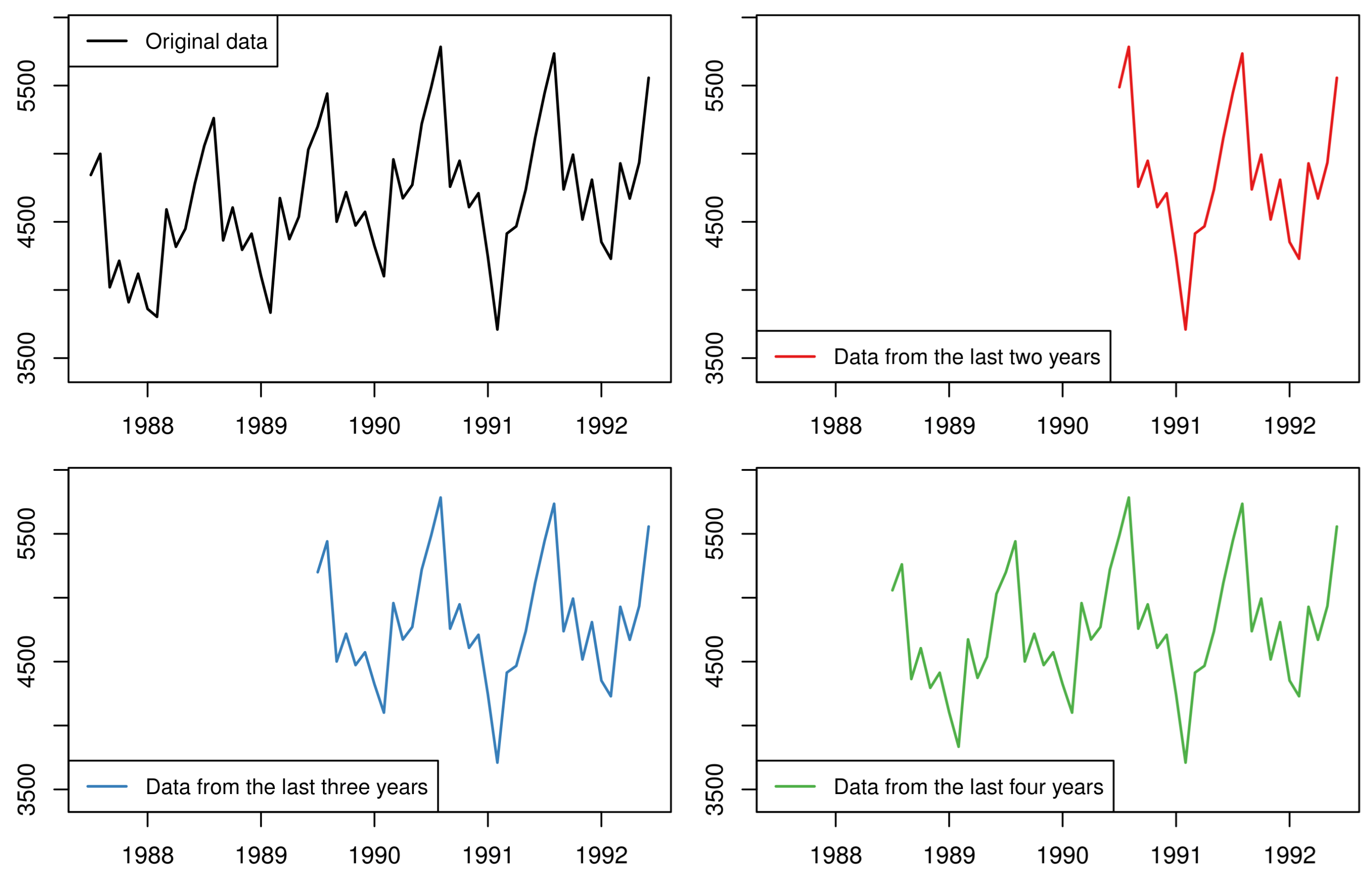
Determining the optimal window of data on which forecasting models are fitted is not a straightforward exercise. Instead, one can consider multiple windows. Assume that a time series consist of n observations. A first set of forecasts can be produced using all n observations. A second set of forecasts can be produced using the most recent observations. This process can be repeated times, such that would still be enough data points for producing forecasts, i.e., at least two seasonal cycles for periodic data. Finally, the multiple sets of forecasts can be combined to obtain the final forecasts. This approach does not transform nor manipulate the original series, but simply trims the beginning of the data to produce multiple overlapping in-sample windows of different lengths based on which forecasts are produced. This approach is known as “forecasting using multiple starting points” (MSP). Figure 5 demonstrates the process of trimming the original series to create new series from multiple starting points.
Research in this stream is limited. To our knowledge, Disney and Petropoulos [18] were the first to empirically examine the approach based on multiple starting points. They applied it on data from the M3 forecasting competition using simple averaging operators (mean, median, and mode), which resulted in improved forecasting performance especially for the yearly frequency. They showed that the improvements generally increase as the number of starting points also increases. They also presented a case study based on the demand of 23 different types of spare parts, showing that forecasting from multiple starting points improves the accuracy in about three-fourths of the cases, with average improvements of about 10%. Bai et al. [19] also empirically investigated this approach, comparing equal versus optimal weights when combining across the forecasts but also considering non-consecutive starting points for their in-sample windows.
We believe that there is scope for more research in this area. Future studies could focus on applying formal techniques for detecting structural changes, which then can be used to select the starting points in a more systematic manner. Another possibility for future investigation could be the application of the concept of multiple starting points within cross-sectional hierarchical structures, where it is usually assumed that every node in the hierarchy has the same number of historical observations. Finally, understanding the circumstances under which forecasting from multiple starting points works best is vital towards implementing it in practice. To our knowledge, there does not exist an open source implementation for forecasting from multiple starting points.
7. Cross-Comparison
The five approaches that were described in the previous five subsections attempt to extract more information from the original time series by performing various forms of data modifications, adjustments, manipulations, and transformations. These can be summarise in three larger categories: random component, frequency, and length. Table 1 summarises how the extraction of information works for each of these five approaches. The theta method retains the frequency and length of the data, but amplifies the local curvatures which are represented as the residuals of a linear regression on trend. MTA transforms the original series through temporal aggregation to new shorter series of lower frequency; inevitably, the upsampling also results in lower noise [40]. Bagging is based on the bootstrapped series that are produced through re-sampling of the remainder from a decomposition process. FOSS focuses on the subsampling of the original series resulting, similar to MAPA, in new series that are shorter and have lower periodicity. Finally, forecasting from multiple starting points is based on trimming the original series by removing the least recent values, retaining the frequency and random component intact.
In Table 2, we map the five approaches with regards to how they handle the three sources of uncertainty: data uncertainty, model form uncertainty, and model parameters uncertainty. Our mapping involves two levels: ✓ denotes full account of that type of uncertainty, while ✓ denotes partial account. The theta method handles the uncertainty in the data in the sense that the local curvatures are amplified or reduced to better identify short and long term movements in the data. MTA also handles data uncertainty as temporal aggregation results in smoothing the noise in the data [40]. However, MTA also addresses the uncertainty in the model form, as different models may be identified as optimal at different temporal levels: a dominating seasonal pattern may lead to the selection of a seasonal-only model at the lowest aggregation level. However, as seasonality is smoothed out by temporal aggregation, a trend pattern may become apparent in a higher aggregation level [11]. Even if the same models are identified as optimal in various temporal levels, then MTA is still likely to help by partially addressing parameters’ uncertainty.
Bagging is the only approach that is able to tackle all three types of uncertainty, something that was extensively discussed by Petropoulos et al. [4]. However, some bagging variations focus on particular sources of uncertainty, as discussed in Section 4. FOSS is the only approach that does not explicitly handle the data uncertainty, but directly focuses on the model form uncertainty (and the model parameters). Finally, MSP tackles data uncertainty in the sense that, by trimming series, outliers or structural changes are removed. However, the new (shorter) series might also result in alternative model forms and sets of parameters.
Next, we consider the computational cost required by each of the approaches to produce forecasts. For simplification, instead of recording computational time per se (as this would depend on length of the series, among others) we compare the various approaches in terms of models required to be fitted. As a benchmark, it is noteworthy that the ets() function of the forecast package for R statistical software fits 19 models (8 for non-seasonal data) before a final model is selected and its forecasts are produced. The theta method is arguably one of the most inexpensive robust time series forecasting methods. In its standard implementation, it requires the fitting of just 2 models, one for each theta line (a simple linear regression model and SES). Even theta variations that consider more than two theta lines, the number of models required is small. The robust implementation by Legaki and Koutsouri [28] that uses a Box-Cox transformation offered, arguably, one of the best trade-offs in performance versus cost in the M4 competition [30].
Compared to theta, all other approaches are more costly. MTA requires forecasts for each aggregation level: 12 for monthly data; 4 for quarterly data. However, this could be slightly reduced when one uses temporal hierarchies (6 for monthly; 3 for quarterly). It is common that in each level an automatic algorithm, like ETS or ARIMA, is used. This means that the number of models required to be fitted increases a lot. Using temporal hierarchies with ETS results in fitting 103 exponential smoothing models for a monthly time series (5 seasonal levels × 19 models + 1 non-seasonal level × 8 models). Empirical evidence https://kourentzes.com/forecasting/2014/10/31/guest-post-on-the-robustness-of-bagging-exponential-smoothing/ (accessed on 1 June 2021) has shown that Bagging’s performance converges when at least 50 bootstrap series are aggregated—while most of the studies consider 100 bootstrap series. This means that Bagging with ETS requires fitting as little as 950 models (50 bootstraps × 19 models) for a single seasonal series and 400 models for a non-seasonal series, rendering it one of the most expensive approaches in this review study. Forecasting with sub-seasonal series is also very costly. From the series created, s of them have a periodicity of 1 with the potentially displaying seasonal patterns. Again assuming ETS, FOSS entails fitting and parametrising 165 models when modelling a series on the quarterly frequency ( models for the sub-series with , plus models for the rest) rising to 2395 models for a monthly time series. The cost for the forecasting from multiple starting points heavily depends on the length of the series. Assuming a monthly time series () with length , we would require at least periods to produce forecasts, which allows us to consider at most 27 starting points, translating to fitting 513 models when using ETS.
Lastly, we consider the performance of the various approaches as published in various studies so far. We focus on the data used in two forecasting competitions, M3 [23] and M4 [29], and particularly the yearly, quarterly, and monthly frequencies. It is important to note that our summary results, presented in Table 3, are based on the empirical evidence presented on other studies, which are identified next to each numerical result. We also limit our results to the values of the symmetric mean absolute percentage error (sMAPE) as reporting the mean absolute scaled error (MASE) was not possible (different researchers apply the scaling differently). For some studies that only provided relative improvements over a benchmark, such as [14], did not differentiate between the results of each competition, such as [41,42], or were limited to one of the two competitions considered, such as [28], we have reproduced the results using the code provided by the corresponding authors. Overall, we observe that some of these approaches are more suited in forecasting non-seasonal patterns (see, for instance, the very good performance of the Box-Cox Theta on the yearly frequency), while others are better when the series are periodic (see, for instance, FOSS and MTA).
Given the high-representativeness of the data in the M3 and M4 datasets [68], we believe that the results can be safely generalised in other settings and contexts, where the presented approaches are expected to work well. However, we will highlight here some particular applications on different contexts. Nikolopoulos et al. [31] apply the theta method on finance data, demonstrating its good performance over other benchmarks. Athanasopoulos et al. [14] offer a case study for the application of MTA (in the form of temporal hierarchies) for forecasting the demand of the Accident and Emergency departments in the UK. Additionally, working with MTA, Yagli et al. [57] improved the performance of solar forecasts. De Oliveira and Cyrino Oliveira [69] demonstrate the effectiveness of the bagging approach on energy consumption data. Finally, the case study of Li et al. [17] also involves high-frequency energy consumption data and shows the good performance of FOSS when complex patterns exist. The application of MSP on different contexts is limited, as this approach has not been—to our knowledge—widely applied yet.
8. Conclusions and a Look to the Future
Univariate time series forecasting can be challenging, especially since real life data do not comply with the assumptions and do not follow data generating processes usually assumed by models that can be found implemented in the forecasting support systems. At the same time, improving forecast accuracy can be crucial, as even a small decrease in the forecast error may translate to significant gains in terms of the utility of the forecasts see, for example, references [33,70], who discuss the case of forecasting for inventories. In this paper, we reviewed five approaches that can enhance the performance of univariate time series forecasting methods. These approaches are based on two basic principles: (i) manipulation of the original data to extract as much information from them as possible, and (ii) forecast combination which has been proved to be extremely beneficial in the forecasting field see, for example, references [71,72].
The five approaches that we presented can be applied on top of established time series forecasting models, such as ETS or ARIMA. In fact, we can argue that all these five approaches work as self-improving mechanisms to boost the performance of the underlying forecasting methods. Although the term “self-improving mechanism” was originally used by Nikolopoulos et al. [38] to describe the performance gained by applying temporal aggregation, we argue that this is a good descriptor for all the approaches discussed in our study. It is important to highlight that the improvements achieved by the application of these approaches do not entail the collection of additional data, such as explanatory variables, that usually come with an additional cost, as well as uncertainty in a sense that, in most cases, the future values of these variables must also be predicted for supporting forecasting methods in a regression fashion. The input for all approaches described is simply the past values of the dependent variable of interest.
When a large number of data are available, then empirical evidence from the latest forecasting competitions [29,73] shows that meta-learning and cross-learning approaches can be used to improve time series forecasting performance. Such “global” approaches are often based of time series features [74] or patterns [75] that may be prevalent and common across many time series. As a result, meta-learning and cross-learning approaches are relevant for companies that require to produce forecasts for myriads of data [76]. Large retailers, such as Walmart, Target, and Carrefour, are representative examples. However, many more companies and organisations are interested in forecasting only a few tens or hundreds of time series to support their operations, marketing, and other functions. As such, “local” solutions, like the ones covered in this study, that use information from singular time series only, are still very useful in practice. More importantly, if one needs to forecast only a small number of series, then it would make sense to invest in the additional computational resources required to handle the most demanding of the approaches (Bagging and FOSS). Regardless, we believe that analysts that wish to apply the approaches presented in this paper should decide based on their added-value across different sampling frequencies (see also the discussions in Section 7) balanced against their relative computational cost.
The various approaches that we presented in this paper have been so far studied in isolation. Although the applying of these approaches in a sequential fashion is entirely feasible, as it is the case with an MTA implementation—the thief() function—which offers theta as one of the methods to produce base forecasts, it would be even more interesting to see future studies that focus on the integration of the approaches described here. The only exception that we are aware of is the study by Wang et al. [77] that attempts to structurally integrate the concepts surrounding the theta method (and the manipulation of the local curvatures) with aspects of non-overlapping temporal aggregation. We believe that there is much scope for further research in integrating “wisdom of the data” approaches. For instance, one could consider defining a temporal hierarchy approach in which the base forecasts for the nodes of a certain aggregation level are not produced by considering the entire series consisting of all information at the same aggregation level, but each node is extrapolated separately using sub-seasonal series (FOSS). Another example would be the integration of bagging and multiple starting points approaches, since each of them focuses on a different way in extracting information from the data.
Another interesting path for future investigation would be to explore how these approaches can better support forecasting in practice. For example, consider the extension of these univariate-oriented approaches to fit within a hierarchical framework which contains several series that are cross-sectionally aggregated. Temporal hierarchies naturally extend to cross-temporal hierarchies, see [56], however this is not the case with all other approaches described here. For instance, when using bagging on a particular node of the hierarchy, the bootstrapping of the remainder could be informed by the remainder of the other nodes. Even more interestingly, a bootstrap model combination approach could be based on the models selected as optimal across hierarchical aggregation levels.
In conclusion, univariate time series forecasting benefits from looking the available data through different lenses, attempting to understand them better and model them more efficiently. This is achieved by tackling uncertainties associated with data itself and easing the identification of an ‘optimal’ model and its parameters. As such, we are looking forward to see more approaches that consider the “wisdom of the data” towards enhancing the forecasting performance.
Author Contributions
Conceptualisation: F.P.; methodology: F.P. and E.S.; software: E.S.; validation: E.S.; visualisation: F.P. and E.S.; formal analysis: F.P. and E.S.; investigation: F.P. and E.S.; resources: F.P. and E.S.; data curation: E.S.; writing—original draft preparation: F.P.; writing—review and editing: E.S.; supervision: F.P.; project administration: F.P.; funding acquisition: F.P. All authors have read and agreed to the published version of the manuscript.
Funding
This research received no external funding.
Institutional Review Board Statement
Not applicable.
Informed Consent Statement
Not applicable.
Data Availability Statement
The data of the M3 and M4 forecasting competitions are publicly available and can be found at https://forecasters.org/resources/time-series-data/, accessed on 1 June 2021.
Acknowledgments
The first author thanks Evelyn and Freddy for their support.
Conflicts of Interest
The authors declare no conflict of interest.
Abbreviations
The following abbreviations are used in this manuscript:
| ARIMA | Auto-regressive Integrated Moving Average |
| ARIMAx | Auto-regressive Integrated Moving Average with Exogenous Variables |
| BMC | Bootstrap Model Combination |
| CBB | Circular Block Bootstrap |
| ETS | Exponential Smoothing |
| ETSx | Exponential Smoothing with Exogenous Variables |
| FOSS | Forecasting with Sub-seasonal Series |
| LPB | Linear Process Bootstrap |
| MAPA | Multiple Temporal Aggregation Algorithm |
| MAPAx | Multiple Temporal Aggregation Algorithm with Exogenous Variables |
| MASE | Mean Absolute Scaled Error |
| MBB | Moving Block Bootstrap |
| MSP | Multiple Starting Points |
| MTA | Multiple Temporal Aggregation |
| SBA | Syntetos-Boylan Approximation |
| SES | Simple Exponential Smoothing |
| sMAPE | Mean Absolute Percentage Error |
| STL | Seasonal and Trend decomposition using Loess |
| THIEF | Temporal Hierarchical Forecasting |
| TSB | Teunter-Syntetos-Babai (method) |
References
- Fildes, R.; Ma, S.; Kolassa, S. Retail forecasting: Research and practice. Int. J. Forecast. 2019. [Google Scholar] [CrossRef] [Green Version]
- Hyndman, R.J.; Koehler, A.B.; Snyder, R.D.; Grose, S. A state space framework for automatic forecasting using exponential smoothing methods. Int. J. Forecast. 2002, 18, 439–454. [Google Scholar] [CrossRef] [Green Version]
- Hyndman, R.; Khandakar, Y. Automatic time series forecasting: The forecast package for R. J. Stat. Softw. 2008, 26, 1–22. [Google Scholar]
- Petropoulos, F.; Hyndman, R.J.; Bergmeir, C. Exploring the sources of uncertainty: Why does bagging for time series forecasting work? Eur. J. Oper. Res. 2018, 268, 545–554. [Google Scholar] [CrossRef]
- Assimakopoulos, V.; Nikolopoulos, K. The Theta model: A decomposition approach to forecasting. Int. J. Forecast. 2000, 16, 521–530. [Google Scholar] [CrossRef]
- Hyndman, R.J.; Billah, B. Unmasking the Theta method. Int. J. Forecast. 2003, 19, 287–290. [Google Scholar] [CrossRef]
- Thomakos, D.; Nikolopoulos, K. Fathoming the theta method for a unit root process. IMA J. Manag. Math. 2012, 25, 105–124. [Google Scholar] [CrossRef] [Green Version]
- Fiorucci, J.A.; Pellegrini, T.R.; Louzada, F.; Petropoulos, F.; Koehler, A.B. Models for optimising the theta method and their relationship to state space models. Int. J. Forecast. 2016, 32, 1151–1161. [Google Scholar] [CrossRef] [Green Version]
- Spiliotis, E.; Assimakopoulos, V.; Nikolopoulos, K. Forecasting with a hybrid method utilizing data smoothing, a variation of the Theta method and shrinkage of seasonal factors. Int. J. Prod. Econ. 2019, 209, 92–102. [Google Scholar] [CrossRef] [Green Version]
- Spiliotis, E.; Assimakopoulos, V.; Makridakis, S. Generalizing the Theta method for automatic forecasting. Eur. J. Oper. Res. 2020, 284, 550–558. [Google Scholar] [CrossRef]
- Kourentzes, N.; Petropoulos, F.; Trapero, J.R. Improving forecasting by estimating time series structural components across multiple frequencies. Int. J. Forecast. 2014, 30, 291–302. [Google Scholar] [CrossRef] [Green Version]
- Petropoulos, F.; Kourentzes, N. Improving forecasting via multiple temporal aggregation. Foresight Int. J. Appl. Forecast. 2014, 34, 12–17. [Google Scholar]
- Petropoulos, F.; Kourentzes, N. Forecast combinations for intermittent demand. J. Oper. Res. Soc. 2015, 66, 914–924. [Google Scholar] [CrossRef] [Green Version]
- Athanasopoulos, G.; Hyndman, R.J.; Kourentzes, N.; Petropoulos, F. Forecasting with temporal hierarchies. Eur. J. Oper. Res. 2017, 262, 60–74. [Google Scholar] [CrossRef] [Green Version]
- Bergmeir, C.; Hyndman, R.J.; Benítez, J.M. Bagging exponential smoothing methods using STL decomposition and Box–Cox transformation. Int. J. Forecast. 2016, 32, 303–312. [Google Scholar] [CrossRef] [Green Version]
- Dantas, T.M.; Cyrino Oliveira, F.L. Improving time series forecasting: An approach combining bootstrap aggregation, clusters and exponential smoothing. Int. J. Forecast. 2018, 34, 748–761. [Google Scholar] [CrossRef]
- Li, X.; Petropoulos, F.; Kang, Y. Improving forecasting with sub-seasonal time series patterns. arXiv 2021, arXiv:2101.00827. [Google Scholar]
- Disney, S.M.; Petropoulos, F. Forecast combinations using multiple starting points. In Proceedings of the Logistics & Operations Management Section Annual Conference (LOMSAC 2015), Glasgow, UK, 12–15 July 2015. [Google Scholar]
- Bai, Y.; Li, X.; Kang, Y. Improving forecasting with multiple starting points. 2021; Unpublished work. [Google Scholar]
- Livera, A.M.D.; Hyndman, R.J.; Snyder, R.D. Forecasting Time Series With Complex Seasonal Patterns Using Exponential Smoothing. J. Am. Stat. Assoc. 2011, 106, 1513–1527. [Google Scholar] [CrossRef] [Green Version]
- Pedregal, D.J.; Trapero, J.R.; Villegas, M.A.; Madrigal, J.J. Submission 260 to the M4 competition. In Github; Universidad de Castilla: Ciudad Real, Spain, 2018. [Google Scholar]
- Dokumentov, A.; Hyndman, R.J. STR: A Seasonal-Trend Decomposition Procedure Based on Regression. arXiv 2020, arXiv:2009.05894. [Google Scholar]
- Makridakis, S.; Hibon, M. The M3-Competition: Results, conclusions and implications. Int. J. Forecast. 2000, 16, 451–476. [Google Scholar] [CrossRef]
- Petropoulos, F.; Nikolopoulos, K. Optimizing Theta Model for Monthly Data. 2013. Available online: https://www.scitepress.org/PublicationsDetail.aspx?ID=PYc+bgnxmJE=&t=1 (accessed on 1 June 2021).
- Petropoulos, F. θ-reflections from the next generation of forecasters. In Forecasting with the Theta Method; Nikolopoulos, K., Thomakos, D.D., Eds.; John Wiley & Sons, Ltd.: Chichester, UK, 2019; pp. 161–175. [Google Scholar] [CrossRef]
- Fioruci, J.A.; Pellegrini, T.R.; Louzada, F.; Petropoulos, F. The Optimised Theta Method. arXiv 2015, arXiv:1503.03529. [Google Scholar]
- Thomakos, D.D.; Nikolopoulos, K. Forecasting Multivariate Time Series with the Theta Method: Multivariate Theta Method. J. Forecast. 2015, 34, 220–229. [Google Scholar] [CrossRef] [Green Version]
- Legaki, N.Z.; Koutsouri, K. Submission 260 to the M4 competition. In Github; National Technical University of Athens: Athens, Greece, 2018. [Google Scholar]
- Makridakis, S.; Spiliotis, E.; Assimakopoulos, V. The M4 Competition: 100,000 time series and 61 forecasting methods. Int. J. Forecast. 2020, 36, 54–74. [Google Scholar] [CrossRef]
- Gilliland, M. The value added by machine learning approaches in forecasting. Int. J. Forecast. 2020, 36, 161–166. [Google Scholar] [CrossRef]
- Nikolopoulos, K.; Thomakos, D.; Petropoulos, F.; Assimakopoulos, V. Theta Model Forecasts for Financial Time Series: A Case Study in the S&P500. Technical Report 0033. 2009. Available online: https://ideas.repec.org/p/uop/wpaper/0033.html (accessed on 1 June 2021).
- Athanasopoulos, G.; Hyndman, R.J.; Song, H.; Wu, D.C. The tourism forecasting competition. Int. J. Forecast. 2011, 27, 822–844. [Google Scholar] [CrossRef]
- Petropoulos, F.; Wang, X.; Disney, S.M. The inventory performance of forecasting methods: Evidence from the M3 competition data. Int. J. Forecast. 2019, 35, 251–265. [Google Scholar] [CrossRef]
- Nikolopoulos, K.; Thomakos, D.D.; Katsagounos, I.; Alghassab, W. On the M4.0 forecasting competition: Can you tell a 4.0 earthquake from a 3.0? Int. J. Forecast. 2020, 36, 203–205. [Google Scholar] [CrossRef]
- Nikolopoulos, K.I.; Thomakos, D.D. Forecasting with The Theta Method: Theory and Applications; John Wiley & Sons: Hoboken, NJ, USA, 2019. [Google Scholar]
- Petropoulos, F.; Nikolopoulos, K. The Theta Method. Foresight Int. J. Appl. Forecast. 2017, 46, 11–17. [Google Scholar]
- Petropoulos, F.; Apiletti, D.; Assimakopoulos, V.; Babai, M.Z.; Barrow, D.K.; Ben Taieb, S.; Bergmeir, C.; Bessa, R.J.; Bijak, J.; Boylan, J.E.; et al. Forecasting: Theory and Practice. arXiv 2021, arXiv:2012.03854. [Google Scholar]
- Nikolopoulos, K.; Syntetos, A.A.; Boylan, J.E.; Petropoulos, F.; Assimakopoulos, V. An aggregate-disaggregate intermittent demand approach (ADIDA) to forecasting: An empirical proposition and analysis. J. Oper. Res. Soc. 2011, 62, 544–554. [Google Scholar] [CrossRef] [Green Version]
- Babai, M.Z.; Ali, M.M.; Nikolopoulos, K. Impact of temporal aggregation on stock control performance of intermittent demand estimators: Empirical analysis. Omega 2012, 40, 713–721. [Google Scholar] [CrossRef]
- Spithourakis, G.; Petropoulos, F.; Nikolopoulos, K.; Assimakopoulos, V. A Systemic View of ADIDA framework. IMA J. Manag. Math. 2014, 25, 125–137. [Google Scholar] [CrossRef] [Green Version]
- Spiliotis, E.; Petropoulos, F.; Assimakopoulos, V. Improving the forecasting performance of temporal hierarchies. PLoS ONE 2019, 14, e0223422. [Google Scholar] [CrossRef] [PubMed] [Green Version]
- Spiliotis, E.; Petropoulos, F.; Kourentzes, N.; Assimakopoulos, V. Cross-temporal aggregation: Improving the forecast accuracy of hierarchical electricity consumption. Appl. Energy 2020, 261, 114339. [Google Scholar] [CrossRef]
- Croston, J.D. Forecasting and Stock Control for Intermittent Demands. Oper. Res. Q. 1972, 23, 289–303. [Google Scholar] [CrossRef]
- Syntetos, A.A.; Boylan, J.E. The accuracy of intermittent demand estimates. Int. J. Forecast. 2005, 21, 303–314. [Google Scholar] [CrossRef]
- Kostenko, A.V.; Hyndman, R.J. A note on the categorization of demand patterns. J. Oper. Res. Soc. 2006, 57, 1256–1257. [Google Scholar] [CrossRef] [Green Version]
- Kourentzes, N.; Petropoulos, F. Forecasting with multivariate temporal aggregation: The case of promotional modelling. Int. J. Prod. Econ. 2016, 181, 145–153. [Google Scholar] [CrossRef] [Green Version]
- Athanasopoulos, G.; Ahmed, R.A.; Hyndman, R.J. Hierarchical forecasts for Australian domestic tourism. Int. J. Forecast. 2009, 25, 146–166. [Google Scholar] [CrossRef] [Green Version]
- Hyndman, R.J.; Ahmed, R.A.; Athanasopoulos, G.; Shang, H.L. Optimal combination forecasts for hierarchical time series. Comput. Stat. Data Anal. 2011, 55, 2579–2589. [Google Scholar] [CrossRef] [Green Version]
- Athanasopoulos, G.; Gamakumara, P.; Panagiotelis, A.; Hyndman, R.J.; Affan, M. Hierarchical Forecasting. In Macroeconomic Forecasting in the Era of Big Data: Theory and Practice; Fuleky, P., Ed.; Springer International Publishing: Cham, Switzerland, 2020; pp. 689–719. [Google Scholar] [CrossRef] [Green Version]
- Hollyman, R.; Petropoulos, F.; Tipping, M.E. Understanding forecast reconciliation. Eur. J. Oper. Res. 2021, 294, 149–160. [Google Scholar] [CrossRef]
- Kourentzes, N.; Rostami-Tabar, B.; Barrow, D.K. Demand forecasting by temporal aggregation: Using optimal or multiple aggregation levels? J. Bus. Res. 2017, 78, 1–9. [Google Scholar] [CrossRef] [Green Version]
- Jeon, J.; Panagiotelis, A.; Petropoulos, F. Probabilistic forecast reconciliation with applications to wind power and electric load. Eur. J. Oper. Res. 2019, 279, 364–379. [Google Scholar] [CrossRef]
- Nystrup, P.; Lindström, E.; Pinson, P.; Madsen, H. Temporal hierarchies with autocorrelation for load forecasting. Eur. J. Oper. Res. 2020, 280, 876–888. [Google Scholar] [CrossRef]
- Kourentzes, N.; Athanasopoulos, G. Elucidate structure in intermittent demand series. Eur. J. Oper. Res. 2021, 288, 141–152. [Google Scholar] [CrossRef]
- Teunter, R.H.; Syntetos, A.A.; Zied Babai, M. Intermittent demand: Linking forecasting to inventory obsolescence. Eur. J. Oper. Res. 2011, 214, 606–615. [Google Scholar] [CrossRef]
- Kourentzes, N.; Athanasopoulos, G. Cross-temporal coherent forecasts for Australian tourism. Ann. Tour. Res. 2019, 75, 393–409. [Google Scholar] [CrossRef]
- Yagli, G.M.; Yang, D.; Srinivasan, D. Reconciling solar forecasts: Sequential reconciliation. Sol. Energy 2019, 179, 391–397. [Google Scholar] [CrossRef]
- Guerrero, V.M. Time-series analysis supported by power transformations. J. Forecast. 1993, 12, 37–48. [Google Scholar] [CrossRef]
- Cleveland, R.B.; Cleveland, W.S.; McRae, J.E.; Terpenning, I. STL: A seasonal-trend decomposition procedure based on loess. J. Off. Stat. 1990, 6, 3–73. [Google Scholar]
- Bandara, K.; Hewamalage, H.; Liu, Y.H.; Kang, Y.; Bergmeir, C. Improving the Accuracy of Global Forecasting Models using Time Series Data Augmentation. arXiv 2020, arXiv:2008.02663. [Google Scholar]
- Kunsch, H.R. The Jackknife and the Bootstrap for General Stationary Observations. Ann. Stat. 1989, 17, 1217–1241. [Google Scholar] [CrossRef]
- Bühlmann, P. Sieve Bootstrap for Time Series. Bernoulli 1997, 3, 123–148. [Google Scholar] [CrossRef]
- Politis, D.N.; Romano, J.P. A Circular Block-Resampling Procedure for Stationary Data; Tech. Rep. No. 370; Department of Statistics, Stanford University: Stanford, CA, USA, 1991. [Google Scholar]
- McMurry, T.; Politis, D.N. Banded and tapered estimates of autocovariance matrices and the linear process bootstrap. J. Time Ser. Anal. 2010, 31, 471–482. [Google Scholar] [CrossRef] [Green Version]
- Dantas, T.M.; Cyrino Oliveira, F.L.; Varela Repolho, H.M. Air transportation demand forecast through Bagging Holt Winters methods. J. Air Transp. Manag. 2017, 59, 116–123. [Google Scholar] [CrossRef]
- Meira, E.; Cyrino Oliveira, F.L.; Jeon, J. Treating and Pruning: New approaches to forecasting model selection and combination using prediction intervals. Int. J. Forecast. 2021, 37, 547–568. [Google Scholar] [CrossRef]
- Pesaran, M.H.; Timmermann, A. Selection of estimation window in the presence of breaks. J. Econom. 2007, 137, 134–161. [Google Scholar] [CrossRef]
- Spiliotis, E.; Kouloumos, A.; Assimakopoulos, V.; Makridakis, S. Are forecasting competitions data representative of the reality? Int. J. Forecast. 2020, 36, 37–53. [Google Scholar] [CrossRef]
- de Oliveira, E.M.; Cyrino Oliveira, F.L. Forecasting mid-long term electric energy consumption through bagging ARIMA and exponential smoothing methods. Energy 2018, 144, 776–788. [Google Scholar] [CrossRef]
- Syntetos, A.A.; Nikolopoulos, K.; Boylan, J.E. Judging the judges through accuracy-implication metrics: The case of inventory forecasting. Int. J. Forecast. 2010, 26, 134–143. [Google Scholar] [CrossRef]
- Bates, J.M.; Granger, C.W.J. The Combination of Forecasts. Oper. Res. Soc. 1969, 20, 451–468. [Google Scholar] [CrossRef]
- Timmermann, A. Forecast Combinations. Handb. Econ. Forecast. 2006, 1, 135–196. [Google Scholar]
- Makridakis, S.; Spiliotis, E.; Assimakopoulos, V. The M5 Accuracy Competition: Results, Findings and Conclusions. 2020. Available online: https://drive.google.com/drive/u/1/folders/1S6IaHDohF4qalWsx9AABsIG1filB5V0q (accessed on 1 June 2021).
- Montero-Manso, P.; Athanasopoulos, G.; Hyndman, R.J.; Talagala, T.S. FFORMA: Feature-based forecast model averaging. Int. J. Forecast. 2020, 36, 86–92. [Google Scholar] [CrossRef]
- Kang, Y.; Spiliotis, E.; Petropoulos, F.; Athiniotis, N.; Li, F.; Assimakopoulos, V. Déjà vu: A data-centric forecasting approach through time series cross-similarity. J. Bus. Res. 2020. [Google Scholar] [CrossRef]
- Seaman, B. Considerations of a retail forecasting practitioner. Int. J. Forecast. 2018, 34, 822–829. [Google Scholar] [CrossRef]
- Wang, B.; Petropoulos, F.; Jooyoung, J.; Erdogan, G. Integrating theta method and multiple temporal aggregation: Optimising aggregation levels. In Proceedings of the 39th International Symposium on Forecasting ISF 2019, Thessaloniki, Greece, 16–19 June 2019. [Google Scholar]
Figure 1.
An illustrative example of producing theta lines for the theta method. The original data (black line) are de-seasonalised (red line). Then, a linear regression on trend produces the theta line with (blue line). The theta line with (green line) has double the curvatures of the seasonally adjusted data.

Figure 2.
A visual example where multiple new temporally aggregated time series are created based on the original data. The monthly data (black line) are temporally aggregated to quarterly (red line), semesterly (blue line), and yearly (green line) data.
Figure 2.
A visual example where multiple new temporally aggregated time series are created based on the original data. The monthly data (black line) are temporally aggregated to quarterly (red line), semesterly (blue line), and yearly (green line) data.
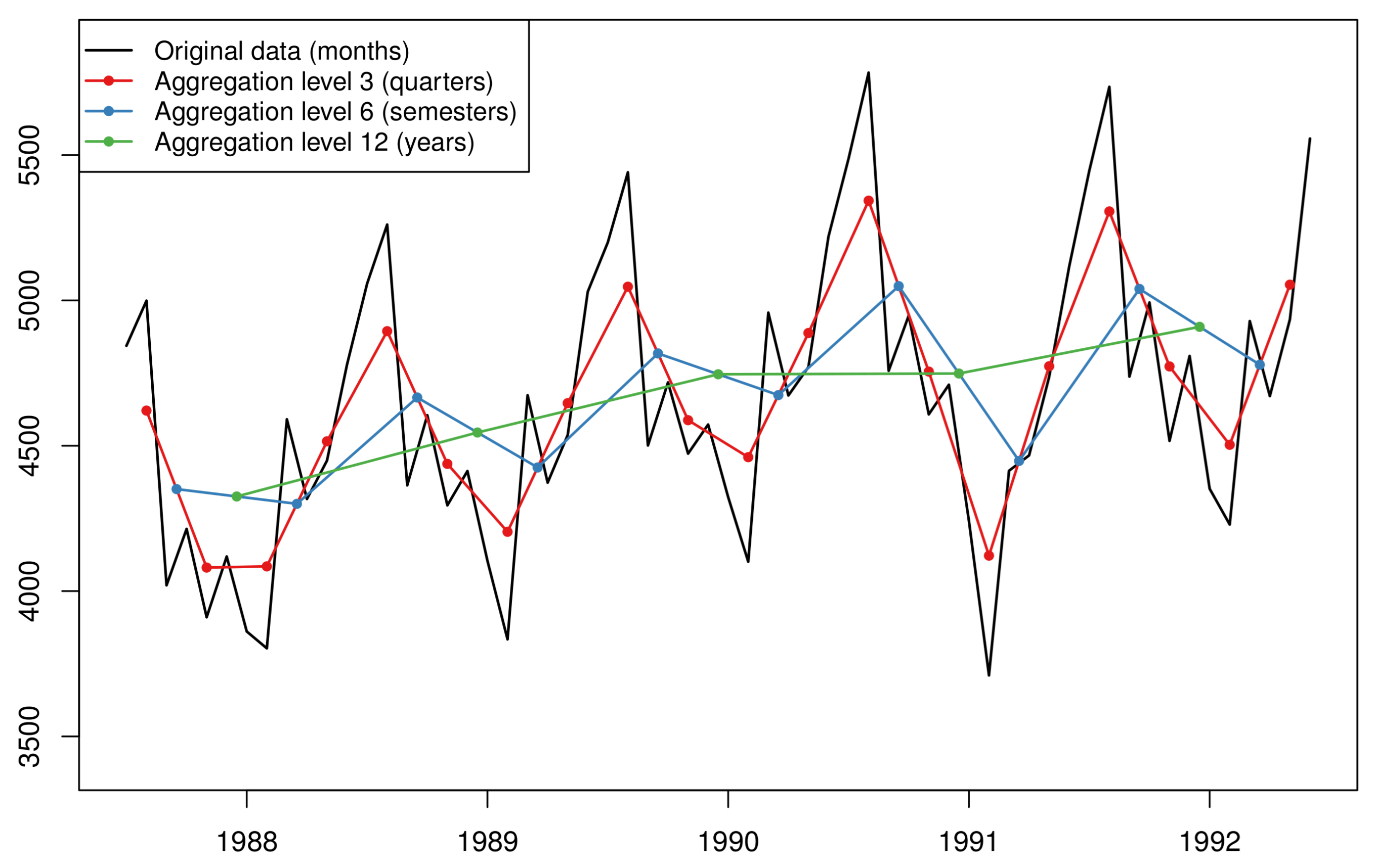
Figure 3.
The original data (black line) together with 30 bootstrapped series (blue lines).
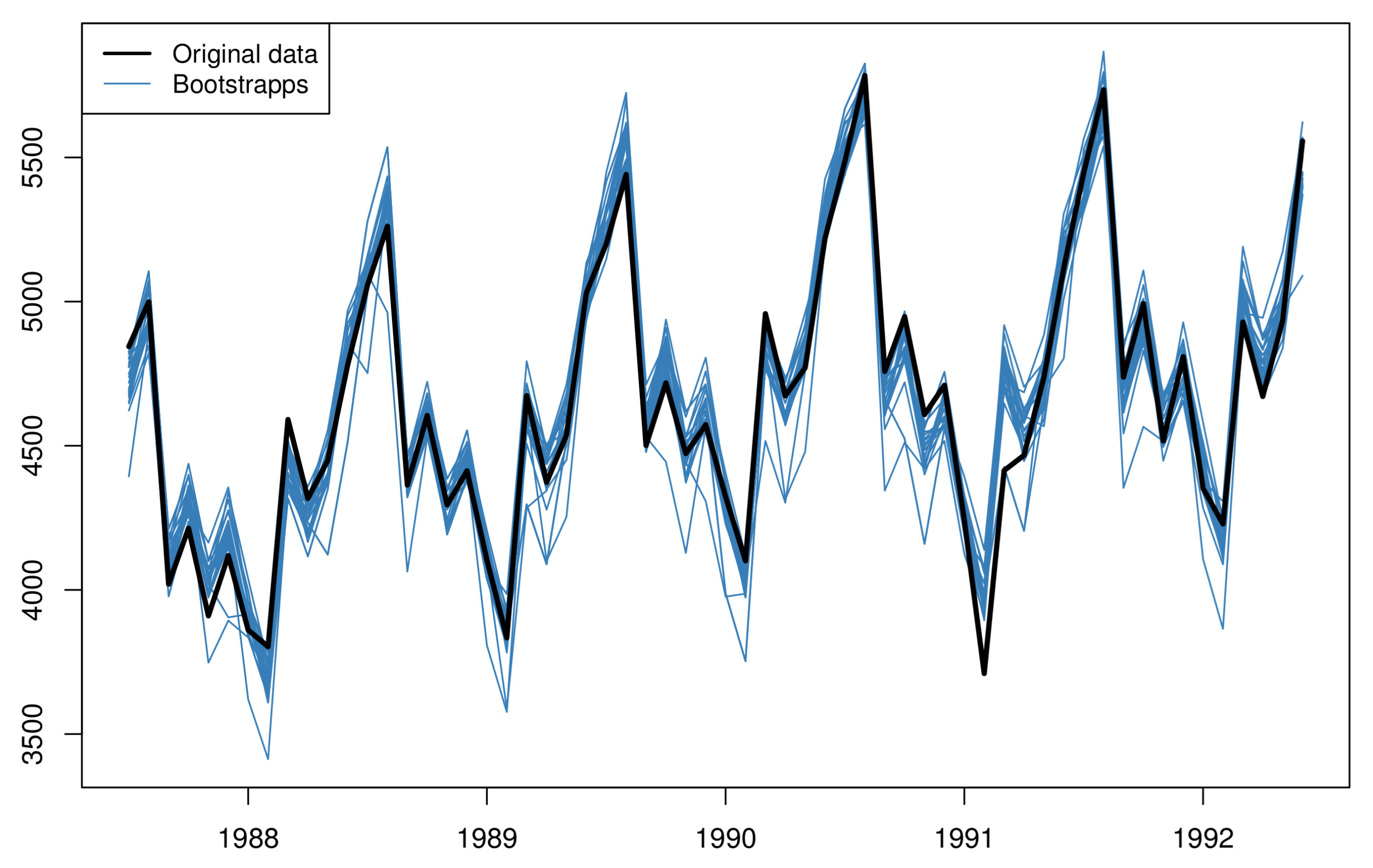
Figure 4.
An illustrative example of producing sub-seasonal series by sub-sampling the original monthly data (first panel). In the second panel, we have produced a non-seasonal series that consists only of the periods in July of each year. The third and fourth panels show two more sub-sampled series with periodicity 2 and 3, respectively. Note that by considering particular subsamples, the level as well as other patterns change significantly.

Figure 5.
An illustrative example of producing series from multiple starting points. The original data (first panel) are trimmed so that the periods from only the last two years (second panel), the last three years (third panel), or the last four years (fourth panel) are considered.
Figure 5.
An illustrative example of producing series from multiple starting points. The original data (first panel) are trimmed so that the periods from only the last two years (second panel), the last three years (third panel), or the last four years (fourth panel) are considered.


Table 1.
How does extraction of the information work?
| Approach | Random Component | Frequency | Length |
|---|---|---|---|
| Theta | ✓ | ||
| MTA | ✓ | ✓ | ✓ |
| Bagging | ✓ | ||
| FOSS | ✓ | ✓ | |
| MSP | ✓ |
Table 2.
How do the five approaches handle the sources of uncertainty?
| Approach | Sources of Uncertainty | ||
|---|---|---|---|
| Data | Model | ||
| Form | Parameters | ||
| Theta | ✓ | ||
| MTA | ✓ | ✓ | ✓ |
| Bagging | ✓ | ✓ | ✓ |
| FOSS | ✓ | ✓ | |
| MSP | ✓ | ✓ | ✓ |
Table 3.
The published average performance of the five approaches on the monthly data from the M3 and M4 competitions.
Table 3.
The published average performance of the five approaches on the monthly data from the M3 and M4 competitions.
| Approach | Variation | M3 | M4 | ||||
|---|---|---|---|---|---|---|---|
| Yearly | Quarterly | Monthly | Yearly | Quarterly | Monthly | ||
| Theta | Standard [5] | 16.90 [23] | 8.96 [23] | 13.85 [23] | 14.59 [29] | 10.31 [29] | 13.00 [29] |
| Optimised [8] | 15.94 [8] | 9.28 [8] | 13.74 [8] | 13.68 | 10.09 | 13.32 | |
| Box-Cox [28] | 16.20 | 9.13 | 13.55 | 13.37 [29] | 10.15 [29] | 13.00 [29] | |
| AutoTheta [42] | 16.02 | 9.18 | 13.86 | 13.80 | 10.13 | 13.13 | |
| Theta-EXP [41] | 16.48 | 8.99 | 13.44 | 14.11 | 10.37 | 13.12 | |
| MTA | MAPA-ETS [11] | 18.37 [11] | 9.63 [11] | 13.69 [11] | 14.88 | 10.27 | 12.97 |
| THIEF-ETS [14] | 17.00 | 9.38 | 13.58 | 15.36 | 10.40 | 12.89 | |
| THIEF-ARIMA [14] | 17.10 | 9.79 | 14.49 | 15.15 | 10.61 | 13.39 | |
| Bagging | MBB-ETS [15] | 17.89 [15] | 10.13 [15] | 13.64 [15] | 14.47 [66] | 10.23 [66] | 13.30 [66] |
| BMC-ETS [4] | 17.15 [4] | 9.56 [4] | 13.79 [4] | 14.94 [66] | 10.08 [66] | 13.07 [66] | |
| Pruned and Treated [66] | 17.36 [66] | 9.74 [66] | 13.61 [66] | 14.49 [66] | 10.22 [66] | 13.27 [66] | |
| FOSS | FOSS-ETS [17] | 9.24 [17] | 13.56 [17] | 10.15 [17] | 12.84 [17] | ||
| FOSS-ARIMA [17] | 9.68 [17] | 14.01 [17] | 10.41 [17] | 12.87 [17] | |||
| MSP | MSP-ETS [18] | 16.90 [18] | 9.79 [18] | 14.00 [18] | |||
THIEF is applied using the “structural” reconciliation approach, while MAPA using the “hybrid” approach with a mean combination operator for aggregating the ETS components at different temporal aggregation levels. Optimised refers to the “Dynamic Optimised Theta Model”. Results are replicated, where required, using the “thief”, “MAPA”, “forecast”, and “forecTheta” packages for R, of versions 0.3, 2.0.4, 8.14, and 2.2, respectively.
Publisher’s Note: MDPI stays neutral with regard to jurisdictional claims in published maps and institutional affiliations. |
© 2021 by the authors. Licensee MDPI, Basel, Switzerland. This article is an open access article distributed under the terms and conditions of the Creative Commons Attribution (CC BY) license (https://creativecommons.org/licenses/by/4.0/).
Share and Cite
MDPI and ACS Style
Petropoulos, F.; Spiliotis, E. The Wisdom of the Data: Getting the Most Out of Univariate Time Series Forecasting. Forecasting 2021, 3, 478-497. https://0-doi-org.brum.beds.ac.uk/10.3390/forecast3030029
AMA Style
Petropoulos F, Spiliotis E. The Wisdom of the Data: Getting the Most Out of Univariate Time Series Forecasting. Forecasting. 2021; 3(3):478-497. https://0-doi-org.brum.beds.ac.uk/10.3390/forecast3030029
Chicago/Turabian StylePetropoulos, Fotios, and Evangelos Spiliotis. 2021. "The Wisdom of the Data: Getting the Most Out of Univariate Time Series Forecasting" Forecasting 3, no. 3: 478-497. https://0-doi-org.brum.beds.ac.uk/10.3390/forecast3030029