
The Effect of Lead-Time Weather Forecast Uncertainty on Outage Prediction Modeling


1
Department of Civil and Environmental Engineering, University of Connecticut, Storrs, CT 06269, USA
2
Eversource Energy Center, University of Connecticut, Storrs, CT 06269, USA
*
Author to whom correspondence should be addressed.
Forecasting 2021, 3(3), 501-516; https://0-doi-org.brum.beds.ac.uk/10.3390/forecast3030031
Submission received: 21 March 2021
/
Revised: 20 June 2021
/
Accepted: 30 June 2021
/
Published: 5 July 2021
Abstract
:Weather-related power outages affect millions of utility customers every year. Predicting storm outages with lead times of up to five days could help utilities to allocate crews and resources and devise cost-effective restoration plans that meet the strict time and efficiency requirements imposed by regulatory authorities. In this study, we construct a numerical experiment to evaluate how weather parameter uncertainty, based on weather forecasts with one to five days of lead time, propagates into outage prediction error. We apply a machine-learning-based outage prediction model on storm-caused outage events that occurred between 2016 and 2019 in the northeastern United States. The model predictions, fed by weather analysis and other environmental parameters including land cover, tree canopy, vegetation characteristics, and utility infrastructure variables exhibited a mean absolute percentage error of 38%, Nash–Sutcliffe efficiency of 0.54, and normalized centered root mean square error of 68%. Our numerical experiment demonstrated that uncertainties of precipitation and wind-gust variables play a significant role in the outage prediction uncertainty while sustained wind and temperature parameters play a less important role. We showed that, while the overall weather forecast uncertainty increases gradually with lead time, the corresponding outage prediction uncertainty exhibited a lower dependence on lead times up to 3 days and a stepwise increase in the four- and five-day lead times.
1. Introduction
Extreme weather is a serious problem for electric distribution utilities, damaging power grid components and causing outages that can result in significant economic disruption and inconvenience for millions of customers [1,2]. Efficient prediction of the power outages that may result from severe weather events is a key to help utility companies in planning their allocations of crew and equipment for faster and more cost-efficient power restoration [3,4,5]. The time window available to utility managers to restore power is short once the power outages occur as regulatory and customer pressure for timely restoration builds up. State regulators typically require that utilities restore power within four days, a timeframe that for major events constitutes a major challenge [6]. Therefore, the ability to forecast outages with lead times of up to several days would give utility managers time to prepare for major outage events.
The use of machine-learning algorithms has been standard practice for predicting power outages in the past two decades [7,8,9,10,11,12,13]. Nateghi et al. used a Bayesian additive regression tree to predict power outages caused from hurricanes and the model showed a root mean squared error (RMSE) of 894 [14]. Nateghi et al. continued this research and used the same data but used a random forest algorithm to develop an hurricane-induced-outage prediction model, which showed an RMSE of 0.76 and 5.91 by grid level [15]. They only used five hurricanes from a power distribution system in the Gulf Coast region of the United States. The weather products were from the commercial weather forecasting service. Liu et al. used a generalized linear mixed model based on 12 hurricanes and 11 ice storms to predict the number of hurricane- and ice-storm-related electric power outages and showed 3.15 and 4.35 square root of the mean-squared errors for Hurricane Charley and the January 2004 ice storm, respectively [16]. The weather data in that study were obtained from the National Oceanic and Atmospheric Administration National Climatic Data Center and Weather Research and Forecasting (WRF). Kabir et al. utilized a quantile regression forest model based on 11 thunderstorms to predict thunderstorm-induced power outages based on weather data from the National Digital Forecast Database [17]. Wanik et al. studied 89 weather-caused outage events in Connecticut from different seasons and used multiple machine-learning methods including boosted gradient tree to predict the power outages, and the gradient boosting model showed a mean APE of 57.2% [18]. Cerrai et al. studied 76 extratropical and 44 convective storms and used multiple machine-learning models for outage prediction, showing a mean absolute percentage error (MAPE) of 65% for the entire dataset, and 80% for the extratropical events [19]. The weather products in the research of Wanik et al. and Cerrai et al. were both from WRF numerical weather prediction simulations. The main input in all outage-forecasting studies has been information on weather conditions such as wind speed, gust, durations of wind speed over certain thresholds, temperature, and precipitation variables, which is combined with land cover variables, vegetation information, and utility infrastructure data. Arguably, the leading cause of power outages is the interaction among severe weather, electric overhead network distribution, and surrounding trees [20]. While the application of the different machine-learning models described in the literature has improved the ability to predict outages in the electric distribution network, we still need to understand how the accuracy of outage forecasts varies at different lead times. Current literature lacks such studies.
Furthermore, given that weather parameters’ uncertainties are key factors limiting model accuracy, we need to understand how weather forecasting uncertainty varies by lead time and how this uncertainty manifests in outage prediction error through its propagation in the complex machine-learning-based outage prediction models [21]. Numerical weather prediction–based [22] forecasting error is caused by uncertainties in the model’s initial conditions [23], boundary conditions [24], physical parameterizations [25], and model errors [26]. All of these factors, and especially the initial-condition errors [27], determine the quality of forecasted weather parameters at the various lead times (up to five days) used in the OPM. Below, we summarize studies in the literature that have investigated errors in high-resolution weather forecasts.
The unbiased forecast root mean square error of 2 m temperature, 10 m wind speed, and 3 h accumulated precipitation for three selected precipitation events increased by 37%, 7%, and 30%, respectively, at forecast lead times ranging from zero hours to four days for COSMO-E weather forecast model [28]. The temperature at 850 hPa for the 3 km Model for Prediction Across Scales (MPAS) ensemble forecasts for 35 events had a bias increase from −0.2 to −1.2 and RMSE from 0.8 to 2.4 for lead times ranging from 0 to 120 h [29]. Slingo and Palmer showed that the root mean square error of the ensemble mean anomaly forecast grew from less than 1 to 70 for forecast lead times ranging from hours to decades [30]. Yang et al. compared the forecast wind speed for 146 storms based on the Weather Research and Forecasting (WRF) and Integrated Community Limited Area Modeling System models, showing that the RMSE for both models increased from zero hours to 54 forecast hours [31]. Using the gridded Bayesian linear regression to improve the deterministic wind speed prediction with the NCAR’s Real-Time Ensemble Forecast System, the authors showed that R-square decreased by 28% and centered root mean square error increased by 38% for lead times ranging from 0 to 48 h [32].
This study devises a numerical experiment to quantify the weather forecast and corresponding outage prediction uncertainty at different lead times and to investigate how errors in the various weather parameters propagate to outage prediction. By applying an outage prediction model on 273 historical weather-caused outage events across three states in northeastern of the United States—Connecticut, Massachusetts, and New Hampshire—we (i) analyzed the differences between numerical weather prediction analysis and forecasts at different lead times based on a subset of events (25); and (ii) subsequently used the remaining record (217 events) to investigate how the uncertainties of weather forecasting and outage prediction errors change at different lead times using zero-hour forecasts as reference. The numerical experiment quantified how uncertainties of weather forecasting propagate into outage prediction modeling for lead times ranging between one and five days. In the next section, we discuss the study area, while Section 3 and Section 4 describe the methods and results. Discussion and conclusions are presented in Section 5 and Section 6.
2. Study Area and Data
Our study focused on the northeastern U.S. region comprising the New England states of Connecticut, Massachusetts, and New Hampshire. The utility companies for these states are Eversource Energy and AVANGRID—United Illuminating, and the study areas covered the territories of Eversource Connecticut (CT), AVANGRID—Connecticut (UI), Eversource West Massachusetts (WMA), Eversource East Massachusetts (EMA), and Eversource New Hampshire (NH). We investigated historical outage events associated with 273 extratropical storms that took place between April 2016 and April 2018 and yielded 252,666 observations, integrating weather variables with information on utility infrastructure, land cover, vegetation, tree canopy, and utility-reported power outages for each storm event and modeling the power outages to a resolution of 1/32 degrees (the resolution of weather data), covering the region. The numerical experiment is based on a subset of the 273 events (217 events between October 2017 and November 2019) for which we used forecasts for lead times ranging from zero hours to five days. The remaining 25 events (in the period October 2017 to April 2018) for which we have available weather analysis and forecasts (hereafter called overlap events) were used to evaluate the validity of zero-hour forecasts as reference for evaluating the uncertainty of the longer-lead-time forecasts.
The weather data used in our study include numerical weather prediction analysis and forecasts from the Global Weather Corporation (GWC) [33]. The forecast data incorporate the outputs from multiple global numerical weather prediction systems such as the Global Forecast System (GFS) produced by the National Centers for Environmental Prediction (NCEP) and the Integrated Forecast System (IFS) produced by the European Centre for Medium-Range Weather Forecasts (ECMWF) and from additional regional and higher-resolution numerical weather prediction models at shorter lead times. GWC uses machine learning to fine-tune the accuracy of the model forecasts based on in situ station observations. We obtained forecasts from the GWC PointWX product, which represents high spatial and temporal resolution weather forecasts globally, every fifteen minutes [34]. This GWC PointWX product includes forecasts with up to 14 days lead time. In this study, we used PointWX weather data across the study domain and the 217 extratropical events for zero up to five days lead times. It is noted that zero-hour forecast in the GWC PointWX product is “forward-error corrected,” ensuring that the forecast at hour zero matches the observations at that time for key variables (temperature and wind speed). For the GWC PointWX weather analysis product, observational data were input into multiple numerical weather prediction model simulations to output the numerical weather prediction analysis at the grid locations of our study area.
Besides the weather variables, we also converted land cover variables generated from the 2016 National Land Cover Database (NLCD) product [35] about forecast categories covering percentages of miscellaneous forest, deciduous forest, and developed area, the distribution of electric infrastructure by percentage, leaf area index (LAI) [36], and tree canopy cover [37], and historical utility-reported power outages gridded at the resolution of the weather variables. A utility-reported power outage is defined as the loss of the electrical power network that breaks the supply to an end user and needs to be repaired, excluding short-term interruptions (less than 5 s) that are automatically corrected by the system-protection device. According to this definition, a single power outage may affect a different number of customers and is reported at the nearest isolating device. The utilities reported the loss of the electrical power network with geospatial information, so we aggregated the numbers of losses of the electrical power network per grid cell reported by outage event.
For vegetation, we extracted information from the United States Forest Service (USFS) geospatial data on tree canopy cover with 30 m resolution, which is derived from multispectral Landsat imagery and other available ground and ancillary information [38]. Containing percentage tree canopy estimates for each pixel across different land covers and types, these data were aggregated into 1/32 degree cells. This variable introduces in the machine-learning model information on trends and patterns of the trees. All explanatory variables used in the OPM are described in Appendix A.
3. Methods
3.1. Numerical Experiment
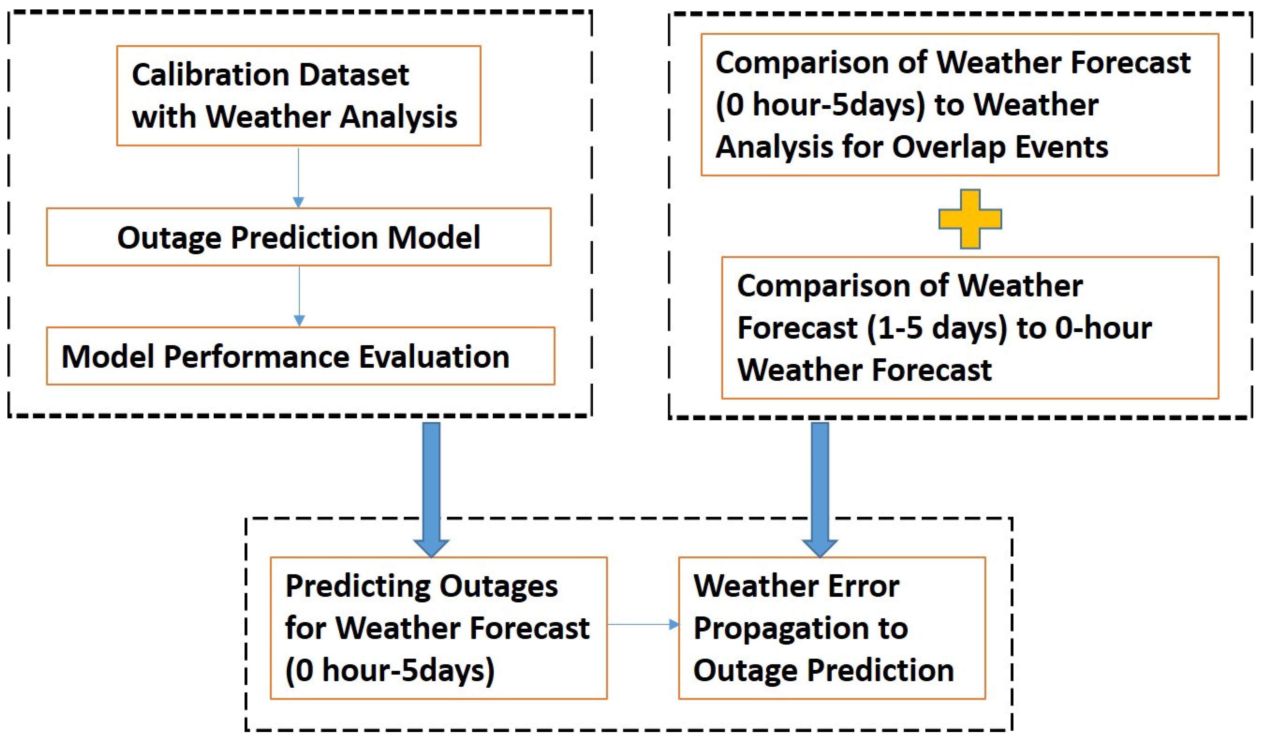
Figure 1 shows a flow chart of the methodology for evaluating the propagation of the uncertainties of weather forecasting to outage forecasting for different lead times. Our experiment had three parts. In the first part, we used input variables and power outages from the 273 historical extratropical storm events to create the OPM. In 2020, Watson et al. covered training data from five service territories (CT, EMA, WMA, NH, and UI), developed a clustering algorithm to summarize the different characteristics of the OPM grid cells, and used RF and BART models to develop an OPM demonstrating an MAPE of 58% to 63% and an NSE of 0.39 to 0.41 [39]. Because some service territories had fewer outage events in the training dataset than others, the inclusion in the training dataset of events from different service territories could benefit the ability of the OPM to predict future events [40,41]. Specifically, a regional OPM using data from different service territories and utilities allowed the study of information from the same or similar storm events in other areas. This approach benefited the areas with limited historical events in the training, potentially giving them better prediction results than they would obtain by running separate OPMs. The details about how to split the data to create the OPM are described in Section 3.2.
In the second part of the experiment, we compared the characteristics of weather analysis and forecast data for the same severe events at different lead times. The forecast included weather at lead times of one to five days (that is, one to five lead days) and of zero hour (zero-hour lead time). The investigation of weather forecast uncertainty had two parts. First, we compared the forecasted weather at different lead times (i.e., from five days to zero hours) with the analysis of weather for overlapping historical storm events. The forecasted weather at lead times with the smallest relative difference was taken into account as the replacement for weather analysis of the forecasted events. We demonstrated that the weather forecast at zero hour had the smallest relative difference to analysis. Moreover, the weather forecast uncertainty at different lead times was quantified in this part. Based on the analysis results from the first part, we compared the weather characteristics of the forecasts at one to five lead days with those of the baseline weather forecast at zero-hour lead time in the second part.
In the third and final part, based on the weather variables of the 217 forecasted events as testing data, we used the created OPM to predict the outages of these forecasted events at the different lead times (1–5 days) and evaluated error performance comparing against the zero-hour weather and outage predictions. This part allowed us to investigate the relationship between the uncertainties of weather forecasting to those of outage prediction modeling to quantify how the weather error propagated to the outage prediction.
3.2. Outage Prediction Model
We structured the OPM using weather analysis (for training) and forecast (for prediction). We used weather, utility infrastructure, land cover, tree canopy, and LAI data described in the previous section and the Appendix A as the input variables and the count of power outages as the target variable. The model outputs are predicted number of outages per grid cell associated with storms in the outage forecasting model, and we counted the outages of all the grids as total outages associated with that storm for each service territory. Since our outage prediction outputs are at the grid level with geospatial information, the utilities could use this information to have a faster and better power restoration management as they know which location would have power outages and how often outages would happen at that location in the coming storms.
We used the historical extratropical events to train a gradient-boosting machine (GBM) model to predict power outages. The GBM model is an ensemble technique that builds several small trees, called “weak learners,” by sequence to correct errors made by previously trained trees and generates a “strong learner” to obtain robust predictive models [42,43]. The GBM focuses on difficult samples and treats the unbalanced data by sequence. The model development began with the determination of three hyperparameters (i.e., tree number, learning rate, and interaction depth) using k-fold cross-validation. The parameter values are 2000 trees, 0.02 learning rate, and 48 for the interaction depth. These hyperparameters were then used to train the GBM model for predicting the number of power outages.
We used “leave one storm out” cross-validation to train the GBM model by holding out the data of a predicted storm from the training dataset. The training dataset comprised the 273 historical extratropical storms. The testing data in this paper were 217 forecasted events at different lead times ranging from zero hours to five days. When we used the created OPM to predict the outages of one forecasted event at different lead times, we held out the data of that forecasted event from the training dataset because there were 25 overlap events with both weather analysis and weather forecast.
Our past research has shown that outage prediction models are sensitive to the extent to which the training data are representative of the severity of the predicted bad weather, and unbalanced dispersed event severity in the training dataset has been shown to cause low accuracy levels [40,41]. After training machine-learning models in the OPM with many different outage ranges to predict events of differing severity, we obtained three optimal ranges for the training datasets: for predicting low-impact events (less than 100 outages), the training dataset comprised all the events with less than 100 outages; for predicting moderate-impact events (100–500 outages), it comprised all historical events; and for predicting high-impact events (more than 500 outages), it comprised all the events with more than 200 outages.
Results from our model cross-validation are shown in Section 4.1. The variable importance of input variables referring to how much GBM “uses” each variable to predict outages is shown in Table 1. As shown in the Table 1, wind-gust, temperature, and precipitation are among the most important variables. The wind duration variables exhibited the least importance in the GBM.
3.3. Performance Evaluation Error Metrics
We used absolute error (AE) to measure the difference between the predicted () and actual () totals of service territory outages from each event (i). The first, second, and third quantiles of the sorted absolute error data (AE Q25, AE Q50, and AE Q75), the first, second, and third quantiles of the sorted absolute percentage error (APE Q25, APE Q50, and APE Q75), mean absolute percentage error (MAPE), Nash–Sutcliffe efficiency (NSE), and normalized centered root mean square error (NCRMSE) were used to determine the bias and random errors. The definition for these performance evaluation error metrics is presented in Appendix B.
Besides the above metrics, we used the weather/outages error metric ratio (NCRMSE Ratio) to evaluate the relationship between the weather uncertainty and outage prediction modeling uncertainty. The NCRMSE ratio was calculated as follows:
As stated in the previous section, zero-hour weather forecast was used as a reference to calculate the 𝑁𝐶𝑅𝑀𝑆𝐸_𝑤𝑒𝑎𝑡ℎ𝑒𝑟𝑉𝑎𝑟𝑖𝑎𝑏𝑙𝑒𝑠, while zero-hour predicted outages were the reference to calculate the 𝑁𝐶𝑅𝑀𝑆𝐸_𝑜𝑢𝑡𝑎𝑔𝑒𝑠. 𝑁𝐶𝑅𝑀𝑆𝐸_𝑤𝑒𝑎𝑡ℎ𝑒𝑟𝑉𝑎𝑟𝑖𝑎𝑏𝑙𝑒𝑠 means the NCRMSE of weather forecast variables for each respective lead time of one to five days to those of zero-hour forecast; and 𝑁𝐶𝑅𝑀𝑆𝐸_𝑜𝑢𝑡𝑎𝑔𝑒𝑠 means the NCRMSE of predicted outages for each respective lead time of one to five days to those of zero-hour forecast.
4. Results
4.1. OPM Model Evaluation
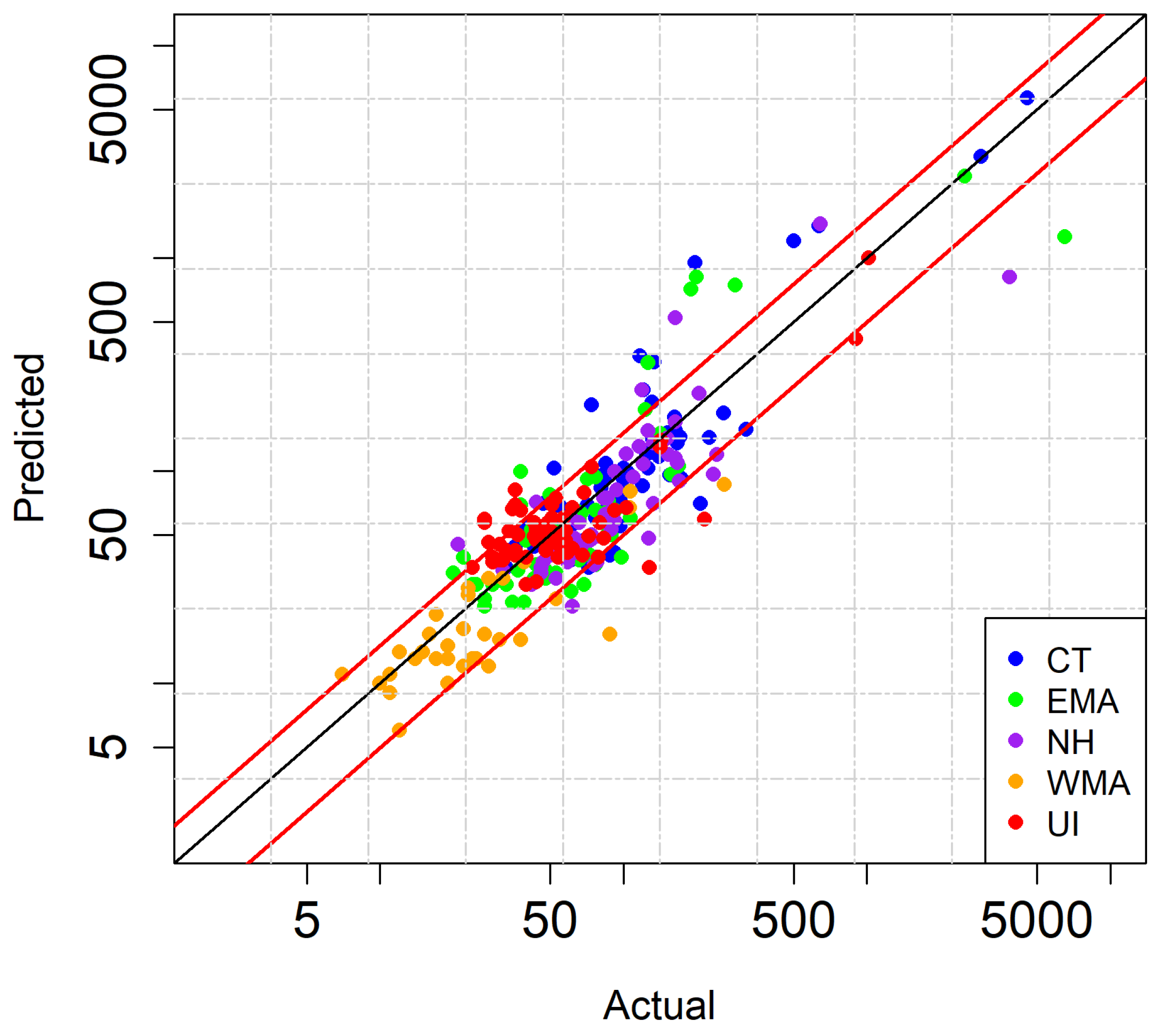
This section discusses the performance of the regional outage prediction model (OPM). Figure 2 shows the validation results of the OPM for the 273 historical events. The vertical and horizontal axes represent the log-scale predicted and actual outages for each event, respectively. The points with different colors corresponds to different regions (blue—CT, green—EMA, purple—NH, orange—WMA, and red—UI). The parallel red lines represent 50 percent model overestimation (top line) and 50 percent model underestimation (bottom line), whereas the black line is the 45 degree line at which predicted and actual agree.
The model evaluation results for the OPM are in Table 2, which shows an MAPE of 38%, NCRMSE of 68%, APE less than 50%, and NSE of 0.54. These model performances are consistent with prior applications of the model [19,39], which indicates that the GWC dataset can be applied for outage modeling. Having established the mode performance, the following sections will discuss the application of the OPM in the numerical experiment. Specifically, we used the model to predict the outages using weather forecasts at different lead times (i.e., the data of forecasted events are used as testing data for the OPM), and we investigated the outage prediction errors at different lead times and how the weather parameter uncertainty propagated into outage prediction error at these lead times.
4.2. Weather and Outage Forecast Uncertainties
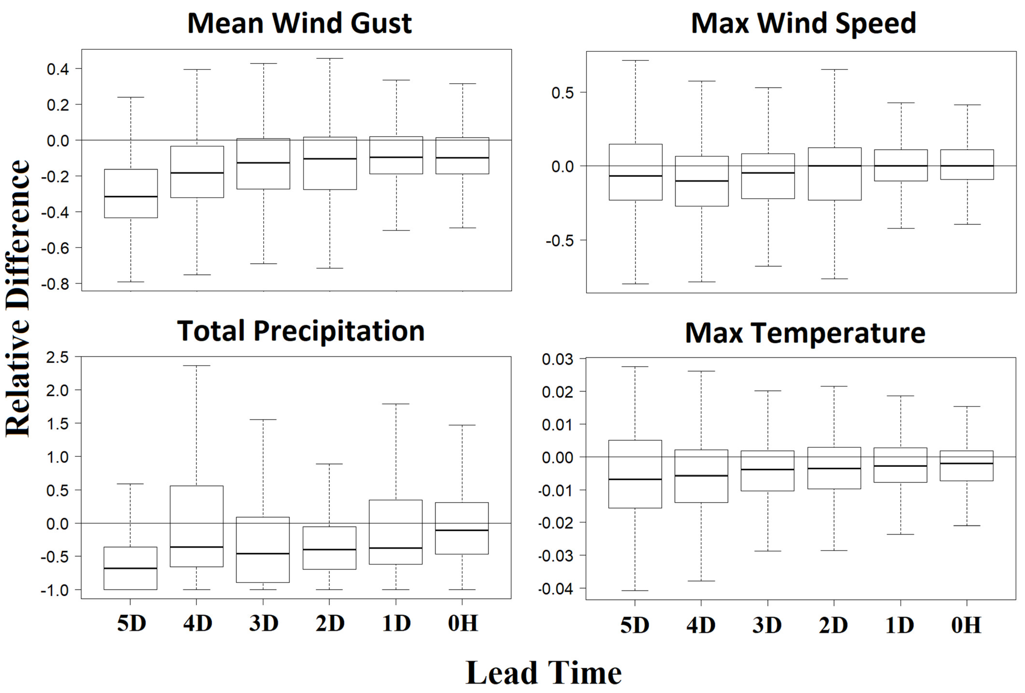
In this section, we used the 25 events with available weather analysis and forecasts, covering lead times from zero hours to five days. We used the weather analysis data as a reference to calculate the relative difference between forecast and analysis for the weather variables of these events. Figure 3 shows the relative differences of forecasted mean wind gust, max wind speed, total precipitation, and max temperature weather variables to their reference weather data for these 25 events at different lead times. In it, 5D-, 4D-, 3D-, 2D-, and 1D-ahead refer to weather forecasts with lead times of five, four, three, two, and one day, respectively, and 0H-ahead refers to the zero-hour forecast. As expected, the relative difference of forecast to analysis decreases for lead times ranging from five days to zero hours, and the zero-hour weather forecast, with the lowest relative difference, is shown to be the closest to the weather analysis. Since observational data of wind speed and temperature were used in the GWC zero-hour wind speed and temperature forecasts, the relative errors of these variables between zero hour and weather analysis were ignored. Therefore, in the subsequent analysis we used the zero-hour forecast, in place of analysis, as a reference to evaluate weather and outage forecasts at one to five day lead times.
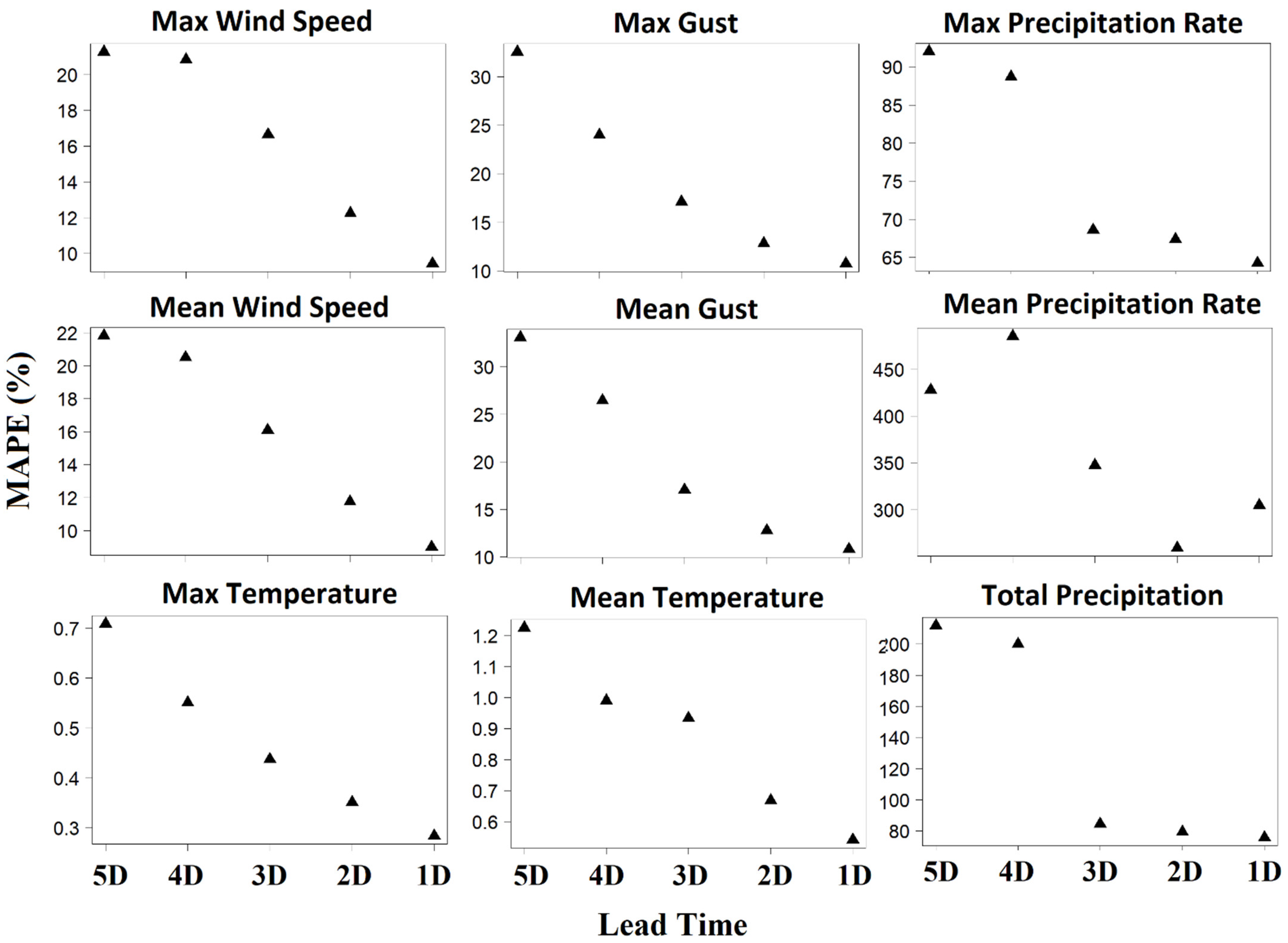
We calculated the mean absolute percentage error (MAPE) between the weather forecasts for the different lead days and the zero-hour weather forecast, for the key weather variables sustained wind, gust, precipitation, and temperature, based on the 217 storms. As Figure 4 shows, the MAPE of weather parameters decreased from five lead days to one, indicating a decreasing trend for weather forecast uncertainty with diminishing lead time. Specifically, for max and mean wind speed, from five to one day lead time, MAPE decreased by nearly 56% and 59%, respectively. For max and mean wind gust, MAPE decreased by 67%. For max and mean temperature, the MAPE decrease was 60% and 56%, respectively, and finally, for mean, max, and total precipitation, MAPE decreased by 29%, 30%, and 64%, respectively. These results indicate a significant effect of lead time on the accuracy of weather parameters used in outage prediction modeling.
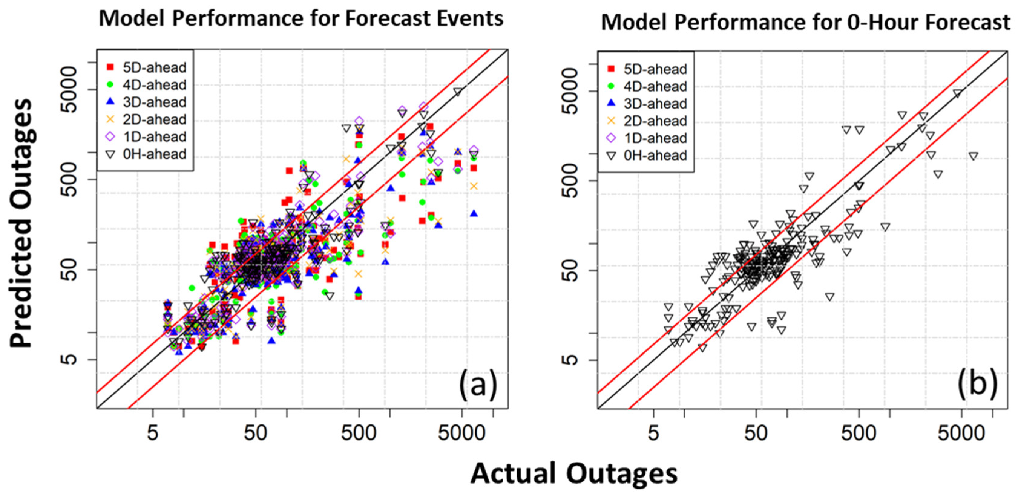
We next investigated the outage prediction modeling uncertainty. We fed the OPM with weather forecasts associated with the 217 events at zero-hour lead time and at one to five lead days to predict outages and compared the results with the actual outages, calculating the error metrics between predicted and actual outages to show the differences in OPM uncertainty. Figure 5a shows the scatter plot of OPM performance for the forecasted weather at the different lead days, while Figure 5b shows the performance for the zero-hour weather forecast. Table 3 shows the values of error metrics AE Q50, MAPE, NCRMSE, and NSE of the model performances for the weather forecasts at different lead times. The performances showed a decreasing trend for AE Q50, MAPE, and NCRMSE and an increasing trend for NSE from five lead days to one, and the performance of outage prediction modeling at zero-hour lead time was better than that at one to five lead days, indicating a decreasing trend for outage prediction modeling uncertainty with diminishing lead time. It is shown that OPM based on the zero-hour forecasted weather was the closest to the OPM performance based on weather analysis, which signifies the use of the zero-hour OPM prediction as reference for the numerical experiment used in this study.
5. Discussion
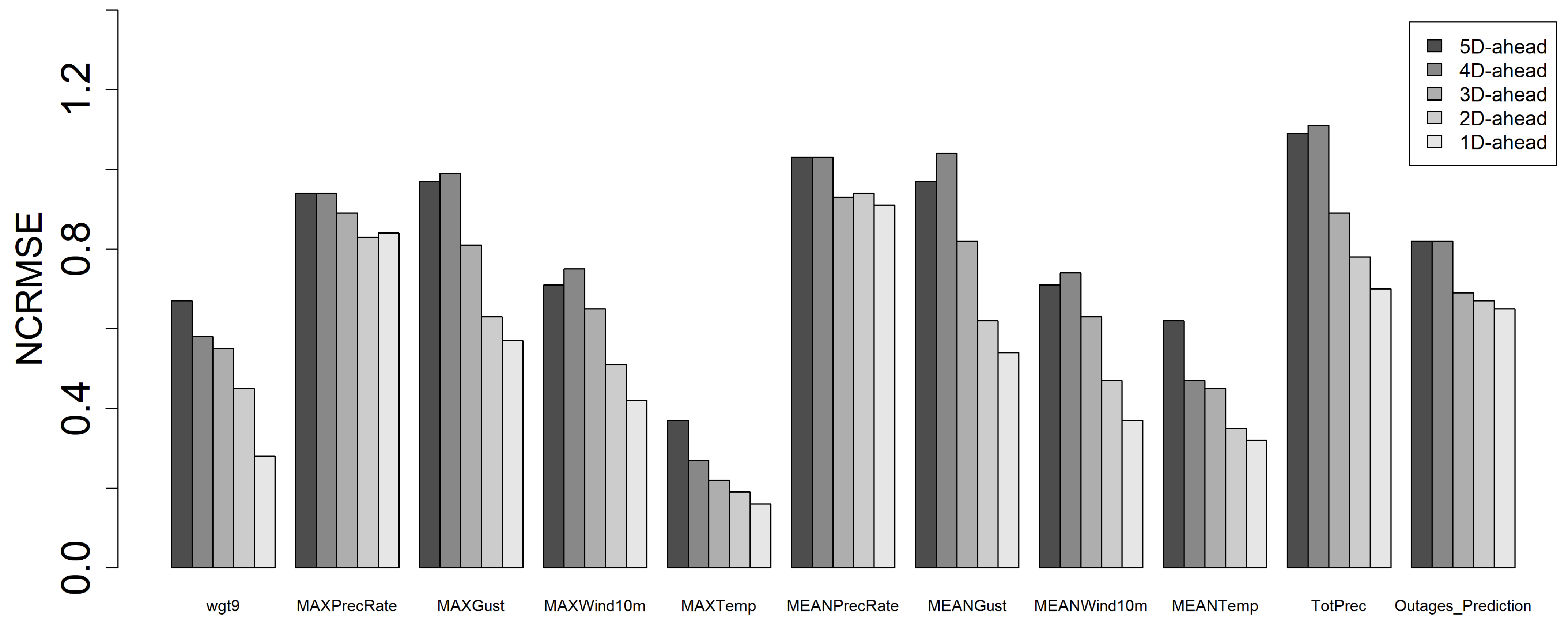
As noted in Section 4.2, the uncertainties of weather forecasts and outage prediction modeling showed increasing trends from one to five days lead time. In this section, we use the results from the numerical experiment to discuss the NCRMSE of the top 10 important weather predictors and the relationship between uncertainties of weather forecasts to outage prediction errors. In Figure 6, the NCRMSE of weather variables and outage predictions shows increasing trends from the one to five days lead time. The NCRMSE increased from 0.56 to 0.97, 0.41 to 0.71, and 0.9 to 1.08 for max gust, max wind speed, and total precipitation, respectively. The temperature variable showed the lowest NCRMSE relative to other weather variables. It is noted that most NCRMSE values (especially precipitation and gust) at four and five days lead times had a significant jump relative to the shorter lead time (1–3 days); this is due to the inclusion of regional weather models starting from 84 h and increasing progressively at shorter lead times. The regional weather models provide both increased spatial and temporal resolution, which is likely the cause for the differences noted in Figure 6. Figure 6 also shows a gradual increase of NCRMSE for the outage predictions between one and three days and a more significant increase in the four-day lead time.
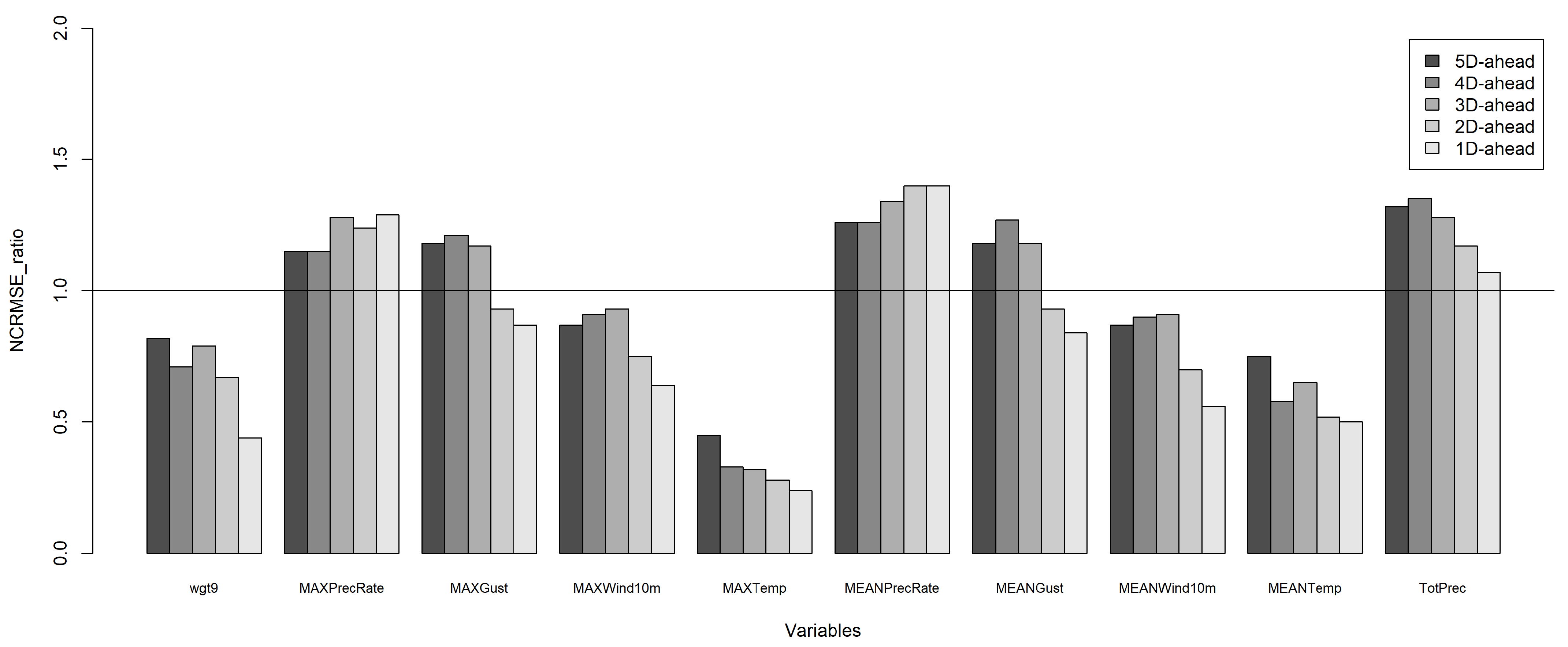
Figure 7 shows the NCRMSE ratio of weather variables to outage prediction for the different lead times, and it shows that precipitation variables had ratios larger than 1 at all lead days, and the mean and max gust variables had a ratio larger than 1 at the lead days of three to five. The other variables such as wind speed, temperature, and wind duration had ratios less than 1 indicating that these variables play a lesser role in the overall outage prediction model’s uncertainty.
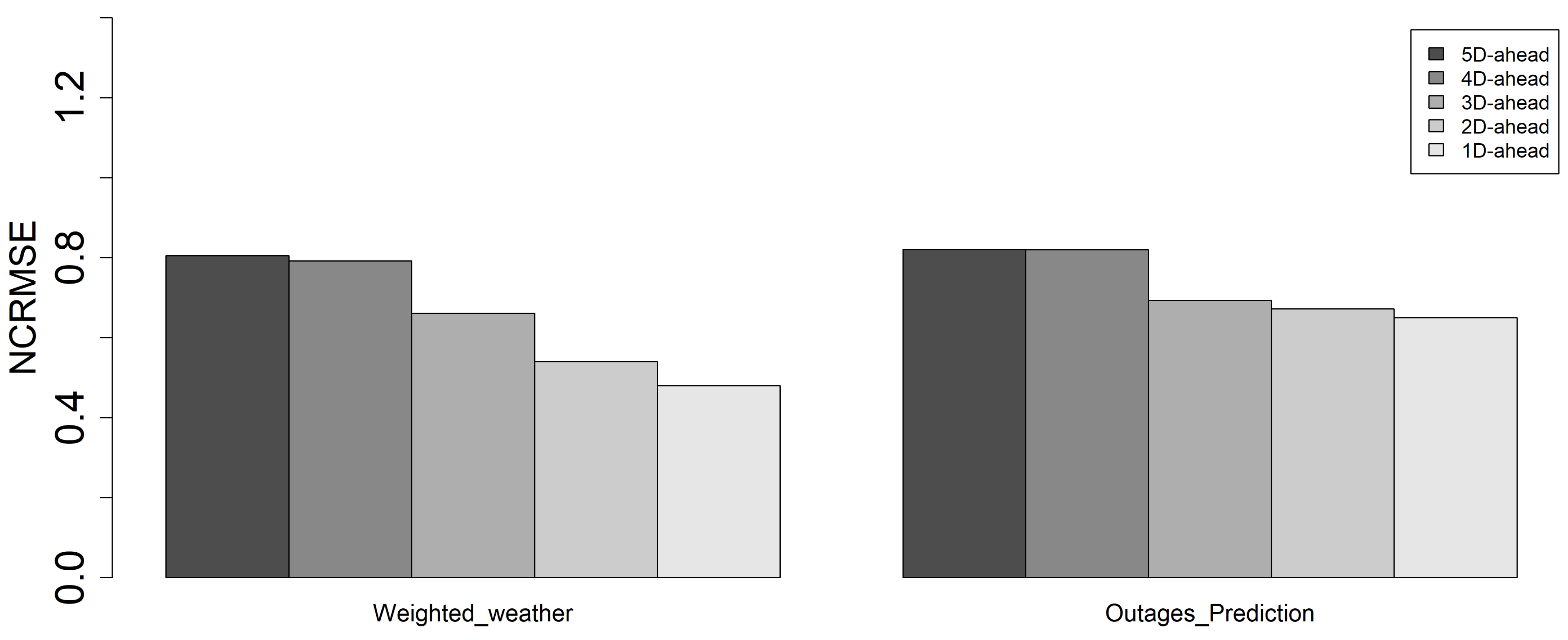
To compare the overall weather forecast uncertainty to the outage prediction uncertainty at different lead times, we calculated the weighted NCRMSE of all-weather variables used in OPM using as weights the variable importance shown in Table 1. The NCRMSE of weighted weather variables is compared against the outage prediction NCRMSE in Figure 8. It is shown that in the long lead times (four and five days), the weather and outage prediction NCRMSEs have similar values indicating that the weather constitutes the main source of uncertainty in the OPM at these lead times. In one to three days lead time, we noted a less gradual increase in the outage prediction NCRMSE relative to the weather forecasts, indicating that OPM modeling can filter some of the increased weather forecasting uncertainty in shorter lead times.
6. Conclusions
This study uses a numerical experiment based on a large number of historical outage events from the northeastern United States to investigate the interactions between weather forecasting and outage prediction modeling uncertainties for lead times between one and five days. Our findings could help electric utilities gain a better understanding of the limitations in storm outage forecasting and be aware of the tradeoffs between outage forecast uncertainty and lead time, allowing for more efficient emergency preparedness and restoration.
The outage prediction model used in our numerical experiment was trained by combining extratropical events that affected five service territories across three states in New England between 2016 and 2019 and exhibited a mean absolute percentage error of 38%, NSE of 0.54, and NCRMSE of 68%. We showed decreasing trends in the weather forecasting uncertainties and outage prediction errors for lead times ranging from five days to one day. The weather uncertainties for precipitation and wind-gust variables played a more important role in the outage prediction error, while sustained wind speed and temperature played a lower role in the outage prediction error. While the weather forecast exhibited a gradual increase of uncertainty from one to five days, outage prediction uncertainty was less dependent on weather forecasting uncertainty in the short (1–3 day) lead times but exhibited a stepwise increase in the four and five days lead forecasts. This behavior of weather uncertainty in outage modeling could guide future improvements in outage prediction, focusing on the implementation of different OPMs for longer-range forecasts (4 and 5 days) versus the one to three days forecasts.
This investigation, based on the Connecticut, Massachusetts, and New Hampshire service territories, needs to be expanded to multiple service territories in the mid-Atlantic and northeastern United States to evaluate the scalability of these results across different vegetation and infrastructure characteristics and weather patterns. Another extension of the study would be to develop statistical error corrections for outage predictions based on predicted uncertainties in weather forecasting at different lead times. This could lead to an ensemble outage-forecasting system that accounts for weather forecasting uncertainty and characteristics of error propagation in outage prediction modeling.
Author Contributions
F.Y. designed the study, developed the model, performed the experiments, analyzed the results, and wrote the manuscript. E.N.A. led the overall project; acquired the funding; co-designed the analysis of results; and contributed to the development of the paper, analysis of results, and manuscript revision. D.C. contributed to co-design the analysis of results and contributed to the development of the paper and manuscript revision. All authors have read and agreed to the published version of the manuscript.
Funding
This work was supported by the DTN LLC and Eversource.
Institutional Review Board Statement
Not applicable.
Informed Consent Statement
Not applicable.
Data Availability Statement
Weather analysis and forecasting data were provided by the Global Weather Corporation. Outage data was were obtained from Eversource Energy and AVANGRID-United Illuminating. We have full access to all the data in this study, and we take complete responsibility for their integrity and the accuracy of the data analysis. Restrictions apply to outage data which can be available obtained from the authors with the permission of Eversource Energy and AVANGRID-United Illuminating.
Acknowledgments
The authors of this publication had research support from DTN LLC and Eversource.
Conflicts of Interest
E.N.A. and D.C. hold stock in Whether Inc.
Appendix A. Explanatory Variables
The utility infrastructure in the Connecticut service territory of Eversource Energy and AVANGRID—United Illuminating contains multiple types of assets, including electric poles and reclosers, among others. We geographically aggregated utility infrastructure data to the 1/32 degree cells of the GWC model’s inner domain and provided three utility infrastructure variables for the OPM: “poles”—that is, a count of poles per 1/32 degree cell; “reclosers”—a count of reclosers per 1/32 degree cell; and “totAssets,” representing the sum of all assets per 1/32 degree cell. Shown in Table A1, these three variables are the most important predictors in a trained OPM, since outages are recorded at the asset level, and the risk of having a reported outage is directly proportional to the number of utility assets.
In this paper, we used variables of wind speed, wind gust, precipitation, and temperature. We determined “MEAN” and “MAX” for each weather variable. The “MAX” variables (such as “MAXWind10m”) represent the 48 h maximum values of each variable, and the “MEAN” variables (such as “MEANGust”) are the mean values of the strongest gusts during a four-hour window. We also used duration and continuous hours of wind at 10 m above different thresholds to represent the wind strength, which was used in the weather variables.
To create the land cover variables, we obtained National Land Cover Database (NLCD) products from the U.S. Geological Survey (USGS). NLCD 2016, published in 2019, these products provide detailed vegetation and urbanization patterns [44]. The percentage of miscellaneous forest, deciduous forest, and developed area at grid level using the land cover product were generated and used in the OPM, which are shown in Table A1. The interaction of trees with overhead lines during storms is the major cause of outages, so we used tree-related land cover variables, which we aggregated into 1/32 degree cells.

Table A1.
Explanatory variables included in the OPM.
| Variables | Abbreviation | Description | Units |
|---|---|---|---|
| Duration of wind at 10 m above 5 m/s | wgt5 | Weather | h |
| Duration of wind at 10 m above 9 m/s | wgt9 | Weather | h |
| Duration of wind at 10 m above 13 m/s | wgt13 | Weather | h |
| Duration of wind at 10 m above 18 m/s | wgt18 | Weather | h |
| Continuous hours of wind above 5 m/s | Cowgt5 | Weather | h |
| Continuous hours of wind above 9 m/s | Cowgt9 | Weather | h |
| Continuous hours of wind above 13 m/s | Cowgt13 | Weather | h |
| Continuous hours of wind above 18 m/s | Cowgt18 | Weather | h |
| Maximum wind speed at 10 m height | Max Wind Speed | Weather | m/s |
| Maximum wind gust | Max Gust | Weather | m/s |
| Maximum precipitation rate | Max Precipitation Rate | Weather | mm/h |
| Maximum temperature | Max Temperature | Weather | K |
| Mean wind at 10 m height | Mean Wind Speed | Weather | m/s |
| Mean wind gust | Mean Gust | Weather | m/s |
| Mean precipitation rate | Mean Precipitation Rate | Weather | mm/h |
| Mean temperature | Mean Temperature | Weather | K |
| Total accumulated precipitation | Tot Precipitation | Weather | mm |
| Percentage of miscellaneous forest | percXFrst | Land cover | % |
| Percentage of deciduous forest | percDecid | Land cover | % |
| Percentage of developed area | percDevel | Land cover | % |
| Count of electric poles | ploes | Infrastructure | count |
| Count of reclosers | reclosers | Infrastructure | count |
| Count of total assets including poles, reclosers, and others | totAssets | Infrastructure | count |
| Average tree canopy percentage around overhead power lines | Avg_treeCanopy | Tree Canopy | % |
| Leaf area index (leaf area/ground area) | LAI | Vegetation | m2/m2 |
Since the seasonal variability of the number of leaves on trees is not explained by land cover variables, we used the weekly climatological leaf area index (LAI, which describes the amount of foliage on the plant) to indicate it. The LAI is based on observations from the Moderate Resolution Imaging Spectroradiometer (MODIS) aboard NASA’s Terra and Aqua satellites, processed to create a weekly climatological product [19,45,46]. We sampled the LAI at the GWC 1/32 degree resolution grid. Historical power outages were reported, with starting times and geographical coordinates, by the utilities’ outage management systems (OMSs). We aggregated and counted the outages during each storm period per 1/32 degree cell and used them as the target variable in the OPM.
Appendix B. Performance Evaluation Error Metrics
We used absolute error (AE) to measure the difference between the predicted () and actual () totals of service territory outages from each event (i). The first, second, and third quantiles of the sorted absolute error data were represented by AE Q25, AE Q50, and AE Q75, respectively. AE was calculated as follows:
The first, second, and third quantiles of the sorted absolute percentage error (APE) data were represented by APE Q25, APE Q50, and APE Q75, respectively. APE was calculated as follows:
We used mean absolute percentage error (MAPE) to measure the mean relative error as a percentage. MAPE was calculated as follows:
We used Nash–Sutcliffe efficiency (NSE), ranging between negative infinity and 1, to determine how well the prediction fit the actual outages. NSE was defined as follows:
We used normalized centered root mean square error (NCRMSE) to quantify the random component of the error. NCRMSE was defined as follows:
References
- Berg, R. Tropical Cyclone Report: Hurricane Ike (al092008), 1–14 September 2008; National Hurricane Center: Miami, FL, USA, 2009.
- Smith, A.; Lott, N.; Houston, T.; Shein, K.; Crouch, J.; Enloe, J. US Billion-Dollar Weather & Climate Disasters: 1980–2017; NOAA National Centers for Environmental Information: Asheville, NC, USA, 2016.
- Duffey, R.B.; Ha, T. Predicting electric power system restoration. In Proceedings of the 2009 IEEE Toronto International Conference Science and Technology for Humanity (TIC-STH), Toronto, ON, Canada, 26–27 September 2009; pp. 666–668. [Google Scholar]
- Duffey, R. Power restoration following major events and disasters. Int. J. Disaster Risk Sci. 2019, 10, 134–148. [Google Scholar] [CrossRef] [Green Version]
- Liu, H.; Davidson, R.A.; Apanasovich, T.V. Statistical Forecasting of electric power restoration times in hurricanes and ice storms. IEEE Trans. Power Syst. 2007, 22, 2270–2279. [Google Scholar] [CrossRef]
- Lubkeman, D.; Julian, D.E. Large scale storm outage management. In Proceedings of the Eighth IEEE International Symposium on Spread Spectrum Techniques and Applications-Programme and Book of Abstracts (IEEE Cat. No.04TH8738), Sydney, NSW, Australia, 30 August–2 September 2004; Institute of Electrical and Electronics Engineers (IEEE): Piscataway, NJ, USA; pp. 16–22. [Google Scholar]
- Arif, A.; Wang, Z. Distribution Network Outage Data Analysis and Repair Time Prediction Using Deep Learning. In Proceedings of the 2018 IEEE International Conference on Probabilistic Methods Applied to Power Systems (PMAPS), Boise, ID, USA, 23–28 June 2018; Institute of Electrical and Electronics Engineers (IEEE): Piscataway, NJ, USA; pp. 1–6. [Google Scholar]
- Eskandarpour, R.; Khodaei, A. Machine learning based power grid outage prediction in response to extreme events. IEEE Trans. Power Syst. 2016, 32, 3315–3316. [Google Scholar] [CrossRef]
- Eskandarpour, R.; Khodaei, A. Leveraging accuracy-uncertainty tradeoff in SVM to achieve highly accurate outage pre-dictions. IEEE Trans. Power Syst. 2017, 33, 1139–1141. [Google Scholar] [CrossRef]
- He, J.; Cheng, M.X. Machine learning methods for power line outage identification. Electr. J. 2021, 34, 106885. [Google Scholar]
- He, J.; Cheng, M.X.; Fang, Y.; Crow, M.L. A machine learning approach for line outage identification in power systems. In Proceedings of the 4th International Conference on Machine Learning, Optimization, and Data Science, LOD 2018, Volterra, Italy, 13–16 September 2018; Springer Science and Business Media LLC: Berlin, Germany, 2019; pp. 482–493. [Google Scholar]
- Reilly, A.C.; Tonn, G.L.; Zhai, C.; Guikema, S.D. Hurricanes and Power System Reliability-The Effects of Individual Decisions and System-Level Hardening. Proc. IEEE 2017, 105, 1429–1442. [Google Scholar] [CrossRef]
- Owerko, D.; Gama, F.; Ribeiro, A. Predicting Power Outages Using Graph Neural Networks. In Proceedings of the 2018 IEEE Global Conference on Signal and Information Processing (GlobalSIP), Anaheim, CA, USA, 26–29 November 2018; pp. 743–747. [Google Scholar]
- Nateghi, R.; Guikema, S.D.; Quiring, S. Comparison and validation of statistical methods for predicting power outage durations in the event of hurricanes. Risk Anal. 2011, 31, 1897–1906. [Google Scholar] [CrossRef]
- Nateghi, R.; Guikema, S.; Quiring, S. Power outage estimation for tropical cyclones: Improved accuracy with simpler models. Risk Anal. 2014, 34, 1069–1078. [Google Scholar] [CrossRef] [PubMed]
- Liu, H.; Davidson, R.A.; Apanasovich, T.V. Spatial generalized linear mixed models of electric power outages due to hurricanes and ice storms. Reliab. Eng. Syst. Saf. 2008, 93, 897–912. [Google Scholar] [CrossRef]
- Kabir, E.; Guikema, S.D.; Quiring, S.M. Predicting thunderstorm-induced power outages to support utility restoration. IEEE Trans. Power Syst. 2019, 34, 4370–4381. [Google Scholar] [CrossRef]
- Wanik, D.; Anagnostou, E.; Hartman, B.; Frediani, M.; Astitha, M. Storm outage modeling for an electric distribution net-work in northeastern USA. Nat. Hazards 2015, 79, 1359–1384. [Google Scholar] [CrossRef]
- Cerrai, D.; Wanik, D.W.; Bhuiyan, A.E.; Zhang, X.; Yang, J.; Frediani, M.E.B.; Anagnostou, E.N.; Bhuiyan, M.E. Predicting storm outages through new representations of weather and vegetation. IEEE Access 2019, 7, 29639–29654. [Google Scholar] [CrossRef]
- Davidson, R.A.; Liu, H.; Sarpong, I.K.; Sparks, P.; Rosowsky, D.V. Electric power distribution system performance in Carolina Hurricanes. Nat. Hazards Rev. 2003, 4, 36–45. [Google Scholar] [CrossRef]
- Dehghanian, P.; Zhang, B.; Dokic, T.; Kezunovic, M. Predictive risk analytics for weather-resilient operation of electric power systems. IEEE Trans. Sustain. Energy 2019, 10, 3–15. [Google Scholar] [CrossRef]
- Mason, B.J. Numerical weather prediction. Contemp. Phys. 1986, 27, 463–472. [Google Scholar] [CrossRef]
- Anthes, R.A. The general question of predictability. In Mesoscale Meteorology and Forecasting; Springer Science and Business Media LLC: Berlin, Germany, 1986; pp. 636–656. [Google Scholar]
- Ying, Y.; Zhang, F. Practical and intrinsic predictability of multiscale weather and convectively coupled equatorial waves during the active phase of an MJO. J. Atmos. Sci. 2017, 74, 3771–3785. [Google Scholar] [CrossRef]
- Grell, G.A.; Kuo, Y.-H.; Pasch, R.J. Semiprognostic Tests of Cumulus Parameterization Schemes in the Middle Latitudes. Mon. Weather Rev. 1991, 119, 5–31. [Google Scholar] [CrossRef] [Green Version]
- Lorenz, E.N. Predictability: A problem partly solved. In Proceedings of the Seminar on Predictability, Reading, UK, 4–8 September 1996. [Google Scholar]
- Kalnay, E. Atmospheric Modeling, Data Assimilation and Predictability; Cambridge University Press (CUP): Cambridge, UK, 2002. [Google Scholar]
- Klasa, C.; Arpagaus, M.; Walser, A.; Wernli, H. An evaluation of the convection-permitting ensemble COSMO-E for three contrasting precipitation events in Switzerland. Q. J. R. Meteorol. Soc. 2018, 144, 744–764. [Google Scholar] [CrossRef]
- Schwartz, C.S. Medium-range convection-allowing ensemble forecasts with a variable-resolution global model. Mon. Weather Rev. 2019, 147, 2997–3023. [Google Scholar] [CrossRef]
- Slingo, J.; Palmer, T. Uncertainty in weather and climate prediction. Philos. Trans. R. Soc. A Math. Phys. Eng. Sci. 2011, 369, 4751–4767. [Google Scholar] [CrossRef]
- Yang, J.; Astitha, M.; Monache, L.D.; Alessandrini, S. An analog technique to improve storm wind speed prediction using a dual NWP model approach. Mon. Weather Rev. 2018, 146, 4057–4077. [Google Scholar] [CrossRef]
- Yang, J.; Astitha, M.; Schwartz, C.S. Assessment of storm wind speed prediction using gridded Bayesian regression applied to historical events with NCAR’s real-time ensemble forecast system. J. Geophys. Res. Atmos. 2019, 124, 9241–9261. [Google Scholar] [CrossRef]
- Global Weather Corporation. Delivering Globally-Available, High-Quality Road-Weather Information. Available online: https://globalweathercorp.com/images/pdf/new-pdf-march-2020/GWC_White_Paper_RoadWX_Quality_May2018.pdf (accessed on 21 March 2021).
- GWC PointWX. Available online: https://globalweathercorp.com/pointwx.html (accessed on 21 March 2021).
- Homer, C.; Dewitz, J.; Jin, S.; Xian, G.; Costello, C.; Danielson, P.; Gass, L.; Funk, M.; Wickham, M.; Stehman, S.; et al. Conterminous United States land cover change patterns 2001–2016 from the 2016 national land cover database. ISPRS J. Photogramm. Remote Sens. 2020, 162, 184–199. [Google Scholar] [CrossRef]
- Myneni, R.B.; Hoffman, S.; Knyazikhin, Y.; Privette, J.L.; Glassy, J.; Tian, Y.; Wang, Y.; Song, X.; Zhang, Y.; Smith, G.R.; et al. Global products of vegetation leaf area and fraction absorbed PAR from year one of MODIS data. Remote Sens. Environ. 2002, 83, 214–231. [Google Scholar] [CrossRef] [Green Version]
- Coulston, J.W.; Jacobs, D.M.; King, C.R.; Elmore, I.C. The Influence of Multi-season Imagery on Models of Canopy Cover. Photogramm. Eng. Remote Sens. 2013, 79, 469–477. [Google Scholar] [CrossRef] [Green Version]
- USGS. NLCD Tree Canopy. 2019. Available online: https://www.usgs.gov/center-news/nlcd-readies-improvements-upcoming-release-2019-product-suite?qt-news_science_products=1#qt-news_science_products (accessed on 21 March 2021).
- Watson, P.L.; Cerrai, D.; Koukoula, M.; Wanik, D.W.; Anagnostou, E. Weather-related power outage model with a growing domain: Structure, performance, and generalisability. J. Eng. 2020, 2020, 817–826. [Google Scholar] [CrossRef]
- Yang, F.; Wanik, D.W.; Cerrai, D.; Bhuiyan, A.E.; Anagnostou, E.N. Quantifying Uncertainty in Machine Learning-Based Power Outage Prediction Model Training: A Tool for Sustainable Storm Restoration. Sustainability 2020, 12, 1525. [Google Scholar] [CrossRef] [Green Version]
- Yang, F.; Watson, P.; Koukoula, M.; Anagnostou, E.N. Enhancing weather-related power outage prediction by event severity classification. IEEE Access 2020, 8, 60029–60042. [Google Scholar] [CrossRef]
- Touzani, S.; Granderson, J.; Fernandes, S. Gradient boosting machine for modeling the energy consumption of commercial buildings. Energy Build. 2018, 158, 1533–1543. [Google Scholar] [CrossRef] [Green Version]
- Natekin, A.; Knoll, A. Gradient boosting machines, a tutorial. Front. Neurorobot. 2013, 7, 21. [Google Scholar] [CrossRef] [Green Version]
- Jin, S.; Homer, C.; Yang, L.; Danielson, P.; Dewitz, J.; Li, C.; Zhu, Z.; Xian, G.; Howard, D. Overall methodology design for the United States national land cover database 2016 products. Remote Sens. 2019, 11, 2971. [Google Scholar] [CrossRef] [Green Version]
- Yang, W.; Tan, B.; Huang, D.; Rautiainen, M.; Shabanov, N.; Wang, Y.; Privette, J.; Huemmrich, K.; Fensholt, R.; Sandholt, I.; et al. MODIS leaf area index products: From validation to algorithm improvement. IEEE Trans. Geosci. Remote Sens. 2006, 44, 1885–1898. [Google Scholar] [CrossRef]
- Gao, F.; Morisette, J.T.; Wolfe, R.E.; Ederer, G.; Pedelty, J.; Masuoka, E.; Myneni, R.; Tan, B.; Nightingale, J. An Algorithm to Produce Temporally and Spatially Continuous MODIS-LAI Time Series. IEEE Geosci. Remote Sens. Lett. 2008, 5, 60–64. [Google Scholar] [CrossRef]
Figure 1.
Flowchart of methodology.

Figure 2.
Actual outages vs. predicted outages for the OPM.

Figure 3.
Relative difference of weather forecast using weather analysis as the reference for overlap events.
Figure 3.
Relative difference of weather forecast using weather analysis as the reference for overlap events.

Figure 4.
MAPE of weather forecast using zero-hour weather forecast as the reference for forecast events (unit: %).
Figure 4.
MAPE of weather forecast using zero-hour weather forecast as the reference for forecast events (unit: %).

Figure 5.
OPM model performance for different lead-time forecast weather for forecast events. (a) Scatter plot of OPM performance for the forecasted weather at lead times from five days to zero hour, (b) Scatter plot of OPM performance for the forecasted weather at zero hour.
Figure 5.
OPM model performance for different lead-time forecast weather for forecast events. (a) Scatter plot of OPM performance for the forecasted weather at lead times from five days to zero hour, (b) Scatter plot of OPM performance for the forecasted weather at zero hour.

Figure 6.
NCRMSE of weather forecast and outage prediction for different lead times.

Figure 7.
NCRMSE ratio of weather variables to outage prediction for different lead times.

Figure 8.
NCRMSE ratio of weighted weather to outage prediction for different lead times.

Table 1.
Variable importance.
| Variables | Importance |
|---|---|
| Max Gust | 17.68 |
| Max Temperature | 11.72 |
| poles | 10.24 |
| totAssets | 8.69 |
| Mean Gust | 6.53 |
| Total Precipitation | 6.32 |
| reclosers | 5.81 |
| percDevel | 3.59 |
| Mean Temperature | 3.54 |
| Max Wind Speed | 3.30 |
| LAI | 2.71 |
| Max Precipitation Rate | 2.64 |
| percDecid | 2.43 |
| wgt9 | 2.33 |
| Mean Wind Speed | 2.19 |
| Mean Precipitation Rate | 2.12 |
| Avg_treeCanopy | 2.11 |
| percXFrst | 1.73 |
| wgt5 | 1.20 |
| Cowgt5 | 1.15 |
| Cowgt9 | 0.77 |
| wgt13 | 0.75 |
| Cowgt13 | 0.25 |
| wgt18 | 0.16 |
| Cowgt18 | 0.04 |
Table 2.
OPM evaluation results.
| Model | AEQ25 | AEQ50 | AEQ75 | APEQ25 | APEQ50 | APEQ75 | MAPE | NCRMSE | NSE |
|---|---|---|---|---|---|---|---|---|---|
| OPM | 7 | 15 | 33 | 12% | 28% | 46% | 38% | 68% | 0.54 |
Table 3.
Model performance of the OPM for forecast weather at different lead times.
| Model | AE Q50 | MAPE | NCRMSE | NSE |
|---|---|---|---|---|
| 0H-ahead | 18 | 49% | 72% | 0.48 |
| 1D-ahead | 18 | 50% | 84% | 0.29 |
| 2D-ahead | 22 | 51% | 86% | 0.24 |
| 3D-ahead | 18 | 48% | 87% | 0.22 |
| 4D-ahead | 21 | 54% | 86% | 0.22 |
| 5D-ahead | 24 | 60% | 87% | 0.21 |
Publisher’s Note: MDPI stays neutral with regard to jurisdictional claims in published maps and institutional affiliations. |
© 2021 by the authors. Licensee MDPI, Basel, Switzerland. This article is an open access article distributed under the terms and conditions of the Creative Commons Attribution (CC BY) license (https://creativecommons.org/licenses/by/4.0/).
Share and Cite
MDPI and ACS Style
Yang, F.; Cerrai, D.; Anagnostou, E.N. The Effect of Lead-Time Weather Forecast Uncertainty on Outage Prediction Modeling. Forecasting 2021, 3, 501-516. https://0-doi-org.brum.beds.ac.uk/10.3390/forecast3030031
AMA Style
Yang F, Cerrai D, Anagnostou EN. The Effect of Lead-Time Weather Forecast Uncertainty on Outage Prediction Modeling. Forecasting. 2021; 3(3):501-516. https://0-doi-org.brum.beds.ac.uk/10.3390/forecast3030031
Chicago/Turabian StyleYang, Feifei, Diego Cerrai, and Emmanouil N. Anagnostou. 2021. "The Effect of Lead-Time Weather Forecast Uncertainty on Outage Prediction Modeling" Forecasting 3, no. 3: 501-516. https://0-doi-org.brum.beds.ac.uk/10.3390/forecast3030031