
Improving Hotel Room Demand Forecasts for Vienna across Hotel Classes and Forecast Horizons: Single Models and Combination Techniques Based on Encompassing Tests

Abstract
:1. Introduction
1.1. Motivation
1.2. Related Literature
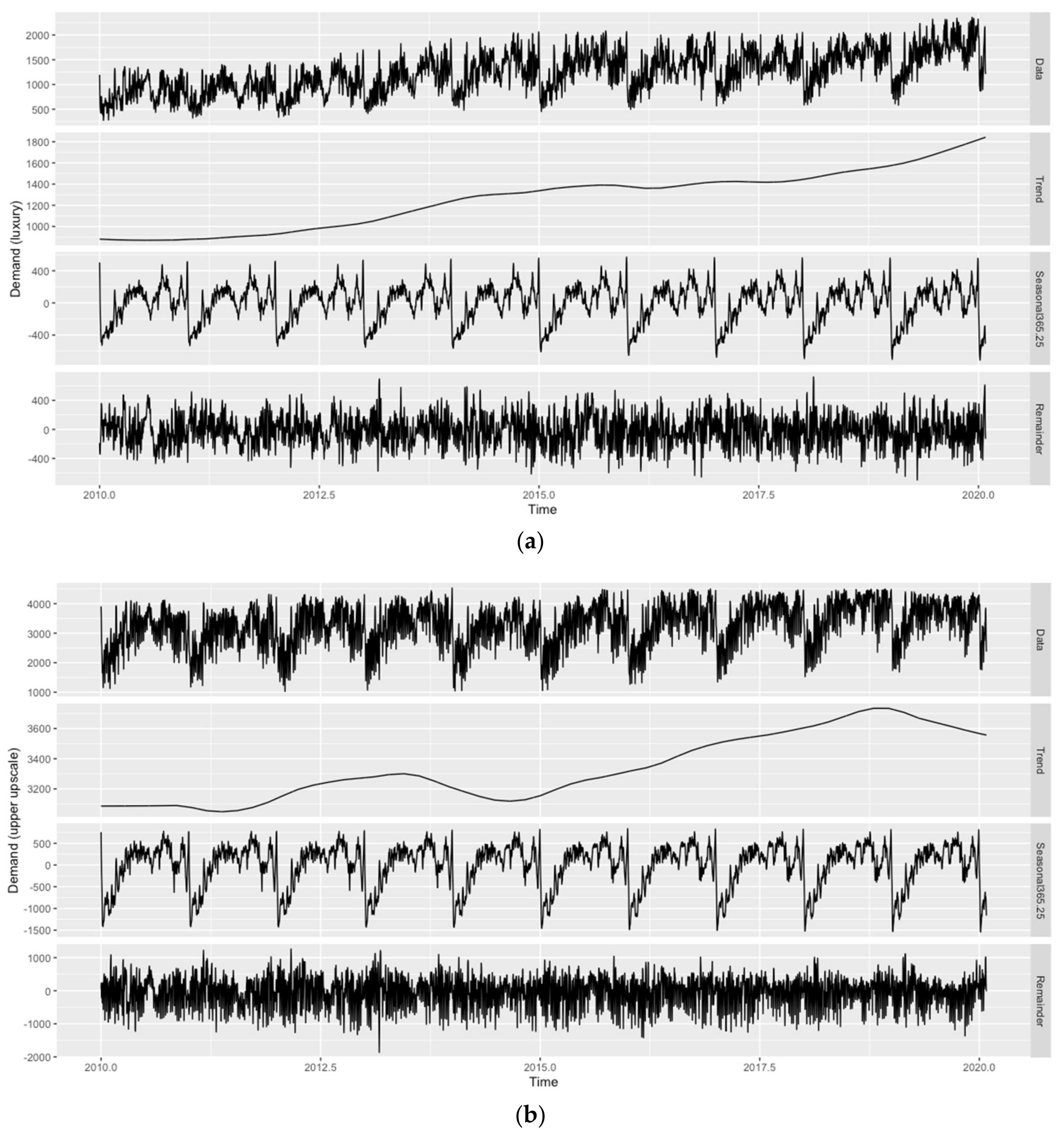
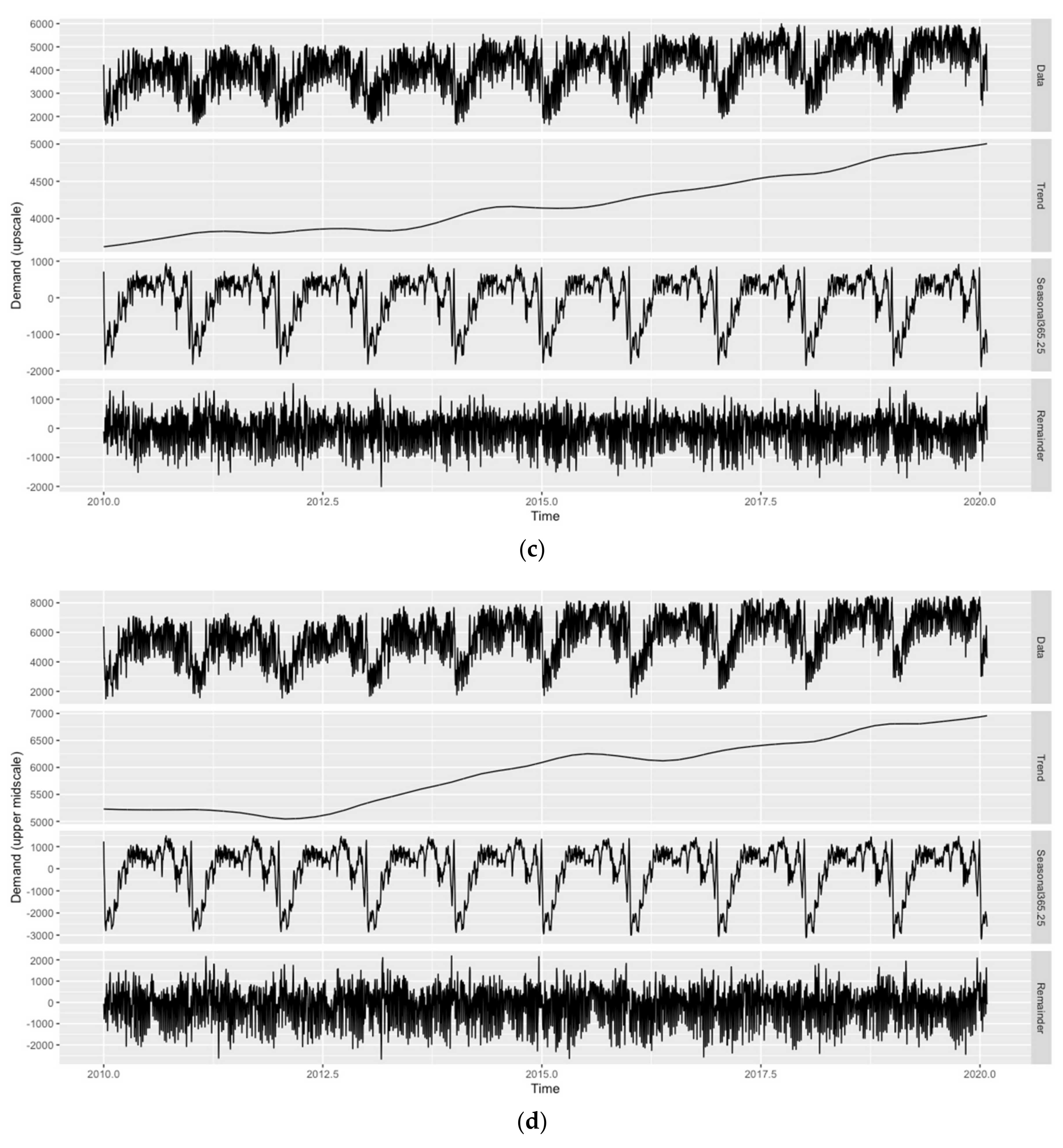
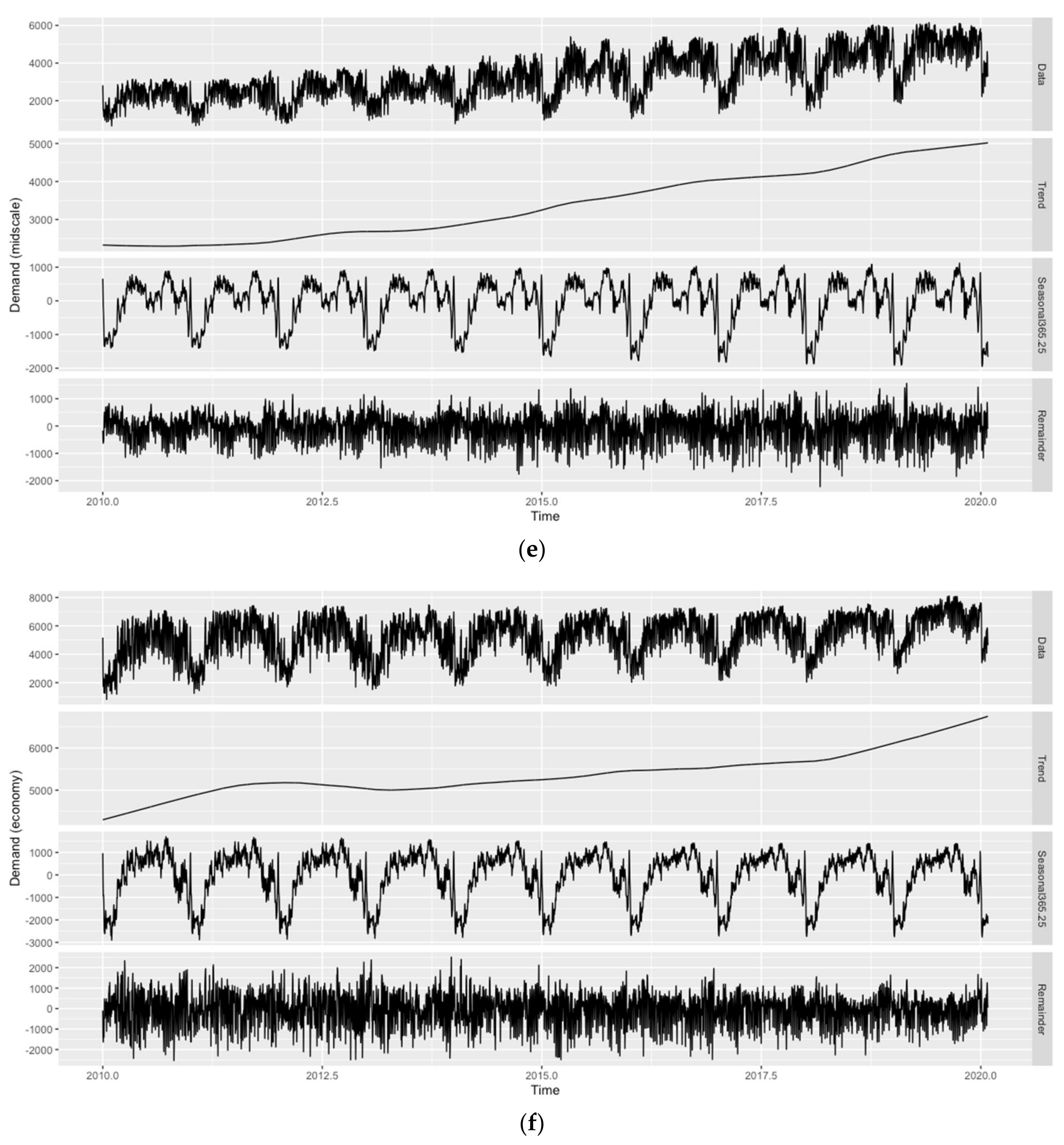
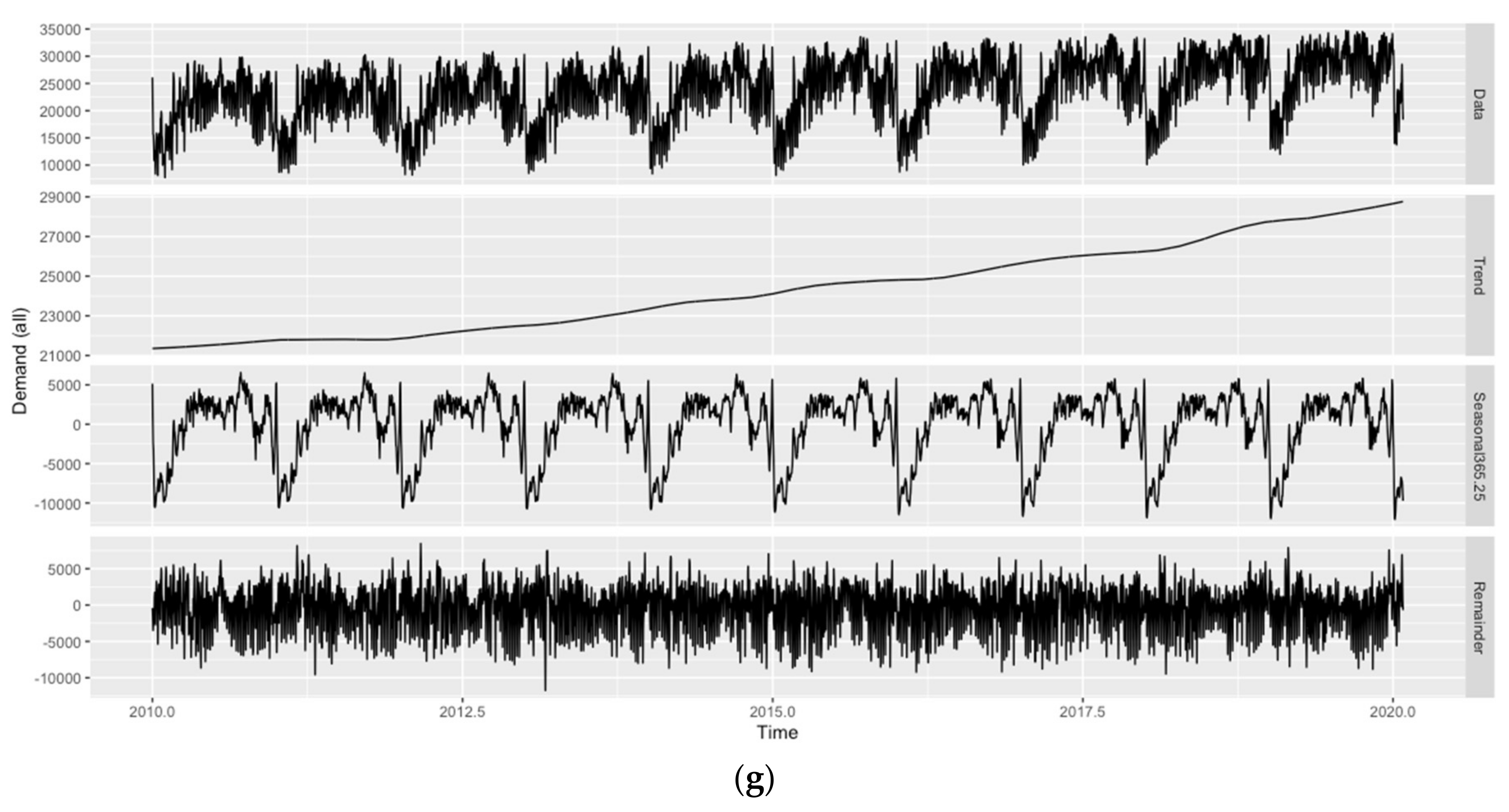
2. Data
3. Methodology
3.1. Forecast Models
3.1.1. Seasonal Naïve
3.1.2. Error Trend Seasonal (ETS)
3.1.3. Seasonal Autoregressive Integrated Moving Average (SARIMA)
3.1.4. Trigonometric Seasonality, Box–Cox Transformation, ARMA Errors, Trend and Seasonal Components (TBATS)
3.1.5. Seasonal Neural Network Autoregression (Seasonal NNAR)
3.1.6. Seasonal NNAR with an External Regressor
3.2. Forecast Combination Techniques
3.2.1. Mean Forecast
3.2.2. Median Forecast
3.2.3. Regression-Based Weights
3.2.4. Bates–Granger Weights
3.2.5. Bates–Granger Ranks
4. Forecasting Procedure and Forecast Evaluation Results
4.1. Forecasting Procedure
4.2. Forecast Evaluation Results
5. Conclusions
Funding
Institutional Review Board Statement
Informed Consent Statement
Data Availability Statement
Acknowledgments
Conflicts of Interest
Appendix A

| h = 1 | Forecast encompassing tests | h = 7 | Forecast encompassing tests | ||||||||||
| Forecast | F-stat | F-prob | Forecast | F-stat | F-prob | ||||||||
| FC_LUXURY_SNAIVE | 16.32009 | 0.0000 | FC_LUXURY_SNAIVE | 12.52591 | 0.0000 | ||||||||
| FC_LUXURY_ETS_1 | 2.85836 | 0.0156 | FC_LUXURY_ETS_7 | 10.00088 | 0.0000 | ||||||||
| FC_LUXURY_SARIMA_1 | 10.92253 | 0.0000 | FC_LUXURY_SARIMA_7 | 16.40607 | 0.0000 | ||||||||
| FC_LUXURY_TBATS_1 | 18.63967 | 0.0000 | FC_LUXURY_TBATS_7 | 8.035354 | 0.0000 | ||||||||
| FC_LUXURY_NNAR_1 | 19.29124 | 0.0000 | FC_LUXURY_NNAR_7 | 20.33636 | 0.0000 | ||||||||
| FC_LUXURY_NNARX_1 | 9.485913 | 0.0000 | FC_LUXURY_NNARX_7 | 20.49514 | 0.0000 | ||||||||
| Forecast accuracy measures | Forecast accuracy measures | ||||||||||||
| Forecast | RMSE | MAE | MAPE (%) | MASE | Sum of ranks | Forecast | RMSE | MAE | MAPE (%) | MASE | Sum of ranks | ||
| FC_LUXURY_SNAIVE | 0.209518 | 0.161318 | 2.15446 | 0.79043 | 44 | FC_LUXURY_SNAIVE | 0.209037 | 0.160055 | 2.138264 | 0.829619 | 33 | ||
| FC_LUXURY_ETS_1 | 0.087544 | 0.064085 | 0.857725 | 0.314005 | 4 | FC_LUXURY_ETS_7 | 0.170569 | 0.123925 | 1.661811 | 0.642345 | 4 | ||
| FC_LUXURY_SARIMA_1 | 0.095704 | 0.071188 | 0.952914 | 0.348809 | 20 | FC_LUXURY_SARIMA_7 | 0.207878 | 0.157969 | 2.113442 | 0.818806 | 29 | ||
| FC_LUXURY_TBATS_1 | 0.191881 | 0.158181 | 2.124453 | 0.775059 | 40 | FC_LUXURY_TBATS_7 | 0.207064 | 0.16589 | 2.225319 | 0.859863 | 34 | ||
| FC_LUXURY_NNAR_1 | 0.109821 | 0.079734 | 1.062345 | 0.390682 | 33 | FC_LUXURY_NNAR_7 | 0.191916 | 0.146502 | 1.947688 | 0.759369 | 24 | ||
| FC_LUXURY_NNARX_1 | 0.108945 | 0.087597 | 1.17971 | 0.42921 | 35 | FC_LUXURY_NNARX_7 | 0.229023 | 0.172272 | 2.29216 | 0.892943 | 43 | ||
| Mean forecast | 0.098279 | 0.077238 | 1.031541 | 0.378453 | 24 | Mean forecast | 0.173872 | 0.131478 | 1.752108 | 0.681494 | 8 | ||
| Median forecast | 0.089816 | 0.06866 | 0.917676 | 0.336422 | 10 | Median forecast | 0.179482 | 0.13769 | 1.833744 | 0.713693 | 19 | ||
| Regression-based weights | 0.107467 | 0.079449 | 1.060927 | 0.389286 | 28 | Regression-based weights | 0.234508 | 0.171612 | 2.284869 | 0.889522 | 41 | ||
| Bates–Granger weights | 0.089893 | 0.069103 | 0.922908 | 0.338592 | 16 | Bates–Granger weights | 0.176806 | 0.133044 | 1.772162 | 0.689612 | 12 | ||
| Bates–Granger ranks | 0.089622 | 0.068704 | 0.917177 | 0.336637 | 10 | Bates–Granger ranks | 0.181203 | 0.135121 | 1.798803 | 0.700377 | 17 | ||
| h = 30 | Forecast encompassing tests | h = 90 | Forecast encompassing tests | ||||||||||
| Forecast | F-stat | F-prob | Forecast | F-stat | F-prob | ||||||||
| FC_LUXURY_SNAIVE | 8.055472 | 0.0000 | FC_LUXURY_SNAIVE | 17.73284 | 0.0000 | ||||||||
| FC_LUXURY_ETS_30 | 17.69353 | 0.0000 | FC_LUXURY_ETS_90 | 7.065177 | 0.0000 | ||||||||
| FC_LUXURY_SARIMA_30 | 55.00696 | 0.0000 | FC_LUXURY_SARIMA_90 | 43.44456 | 0.0000 | ||||||||
| FC_LUXURY_TBATS_30 | 2.085499 | 0.0679 | FC_LUXURY_TBATS_90 | 25.83146 | 0.0000 | ||||||||
| FC_LUXURY_NNAR_30 | 23.52884 | 0.0000 | FC_LUXURY_NNAR_90 | 8.878909 | 0.0000 | ||||||||
| FC_LUXURY_NNARX_30 | 16.90916 | 0.0000 | FC_LUXURY_NNARX_90 | 25.27719 | 0.0000 | ||||||||
| Forecast accuracy measures | Forecast accuracy measures | ||||||||||||
| Forecast | RMSE | MAE | MAPE (%) | MASE | Sum of ranks | Forecast | RMSE | MAE | MAPE (%) | MASE | Sum of ranks | ||
| FC_LUXURY_SNAIVE | 0.213606 | 0.163953 | 2.18938 | 0.95581 | 28 | FC_LUXURY_SNAIVE | 0.231818 | 0.180371 | 2.409105 | 1.450767 | 32 | ||
| FC_LUXURY_ETS_30 | 0.185534 | 0.141494 | 1.895716 | 0.824879 | 4 | FC_LUXURY_ETS_90 | 0.204164 | 0.155037 | 2.067238 | 1.247 | 21 | ||
| FC_LUXURY_SARIMA_30 | 0.335021 | 0.302819 | 4.019495 | 1.765369 | 44 | FC_LUXURY_SARIMA_90 | 0.468366 | 0.438595 | 5.809883 | 3.527725 | 44 | ||
| FC_LUXURY_TBATS_30 | 0.215911 | 0.171995 | 2.302796 | 1.002693 | 32 | FC_LUXURY_TBATS_90 | 0.236342 | 0.191731 | 2.562032 | 1.542139 | 36 | ||
| FC_LUXURY_NNAR_30 | 0.201226 | 0.153374 | 2.036935 | 0.894137 | 12 | FC_LUXURY_NNAR_90 | 0.17141 | 0.131833 | 1.764189 | 1.060365 | 4 | ||
| FC_LUXURY_NNARX_30 | 0.232117 | 0.188084 | 2.492954 | 1.096489 | 40 | FC_LUXURY_NNARX_90 | 0.203281 | 0.166045 | 2.214327 | 1.33554 | 23 | ||
| Mean forecast | 0.196003 | 0.160388 | 2.130115 | 0.935027 | 22 | Mean forecast | 0.213697 | 0.178811 | 2.371894 | 1.43822 | 28 | ||
| Median forecast | 0.194566 | 0.157631 | 2.095555 | 0.918954 | 18 | Median forecast | 0.190474 | 0.154669 | 2.058517 | 1.24404 | 16 | ||
| Regression-based weights | 0.229081 | 0.183769 | 2.437347 | 1.071333 | 36 | Regression-based weights | 0.399399 | 0.374997 | 5.017681 | 3.016191 | 40 | ||
| Bates–Granger weights | 0.196449 | 0.157564 | 2.092582 | 0.918564 | 17 | Bates–Granger weights | 0.180765 | 0.143159 | 1.904875 | 1.151462 | 8 | ||
| Bates–Granger ranks | 0.192562 | 0.153455 | 2.03924 | 0.894609 | 11 | Bates–Granger ranks | 0.186505 | 0.149609 | 1.988532 | 1.203341 | 12 |
| h = 1 | Forecast encompassing tests | h = 7 | Forecast encompassing tests | ||||||||||
| Forecast | F-stat | F-prob | Forecast | F-stat | F-prob | ||||||||
| FC_UPPER_UPSCALE_SNAIVE | 12.59821 | 0.0000 | FC_UPPER_UPSCALE_SNAIVE | 3.392179 | 0.0055 | ||||||||
| FC_UPPER_UPSCALE_ETS_1 | 31.43229 | 0.0000 | FC_UPPER_UPSCALE_ETS_7 | 12.89008 | 0.0000 | ||||||||
| FC_UPPER_UPSCALE_SARIMA_1 | 14.70312 | 0.0000 | FC_UPPER_UPSCALE_SARIMA_7 | 36.16254 | 0.0000 | ||||||||
| FC_UPPER_UPSCALE_TBATS_1 | 32.66598 | 0.0000 | FC_UPPER_UPSCALE_TBATS_7 | 11.18837 | 0.0000 | ||||||||
| FC_UPPER_UPSCALE_NNAR_1 | 42.66397 | 0.0000 | FC_UPPER_UPSCALE_NNAR_7 | 23.78411 | 0.0000 | ||||||||
| FC_UPPER_UPSCALE_NNARX_1 | 32.5047 | 0.0000 | FC_UPPER_UPSCALE_NNARX_7 | 21.28089 | 0.0000 | ||||||||
| Forecast accuracy measures | Forecast accuracy measures | ||||||||||||
| Forecast | RMSE | MAE | MAPE (%) | MASE | Sum of ranks | Forecast | RMSE | MAE | MAPE (%) | MASE | Sum of ranks | ||
| FC_UPPER_UPSCALE_SNAIVE | 0.150782 | 0.110127 | 1.355925 | 0.700727 | 40 | FC_UPPER_UPSCALE_SNAIVE | 0.151458 | 0.110214 | 1.357374 | 0.72622 | 35 | ||
| FC_UPPER_UPSCALE_ETS_1 | 0.127043 | 0.090924 | 1.118678 | 0.57854 | 32 | FC_UPPER_UPSCALE_ETS_7 | 0.129237 | 0.092119 | 1.133693 | 0.606988 | 20 | ||
| FC_UPPER_UPSCALE_SARIMA_1 | 0.082216 | 0.061995 | 0.761406 | 0.394468 | 4 | FC_UPPER_UPSCALE_SARIMA_7 | 0.147454 | 0.10595 | 1.305618 | 0.698123 | 28 | ||
| FC_UPPER_UPSCALE_TBATS_1 | 0.169696 | 0.130443 | 1.604181 | 0.829996 | 44 | FC_UPPER_UPSCALE_TBATS_7 | 0.176288 | 0.133954 | 1.647736 | 0.882647 | 41 | ||
| FC_UPPER_UPSCALE_NNAR_1 | 0.09789 | 0.064829 | 0.798285 | 0.412501 | 13 | FC_UPPER_UPSCALE_NNAR_7 | 0.136968 | 0.094979 | 1.170773 | 0.625834 | 24 | ||
| FC_UPPER_UPSCALE_NNARX_1 | 0.141889 | 0.100997 | 1.251798 | 0.642634 | 36 | FC_UPPER_UPSCALE_NNARX_7 | 0.167772 | 0.140907 | 1.714852 | 0.928461 | 43 | ||
| Mean forecast | 0.100858 | 0.069609 | 0.859669 | 0.442915 | 23 | Mean forecast | 0.117539 | 0.08629 | 1.062078 | 0.56858 | 10 | ||
| Median forecast | 0.103047 | 0.068461 | 0.84682 | 0.435611 | 22 | Median forecast | 0.115785 | 0.083706 | 1.031675 | 0.551554 | 4 | ||
| Regression-based weights | 0.103007 | 0.069989 | 0.864106 | 0.445333 | 27 | Regression-based weights | 0.15941 | 0.109911 | 1.354395 | 0.724223 | 33 | ||
| Bates–Granger weights | 0.094567 | 0.064543 | 0.797838 | 0.410681 | 8 | Bates–Granger weights | 0.11867 | 0.086254 | 1.062423 | 0.568343 | 10 | ||
| Bates–Granger ranks | 0.09646 | 0.06613 | 0.817481 | 0.420779 | 15 | Bates–Granger ranks | 0.119586 | 0.08653 | 1.066684 | 0.570162 | 16 | ||
| h = 30 | Forecast encompassing tests | h = 90 | Forecast encompassing tests | ||||||||||
| Forecast | F-stat | F-prob | Forecast | F-stat | F-prob | ||||||||
| FC_UPPER_UPSCALE_SNAIVE | 3.355434 | 0.0060 | FC_UPPER_UPSCALE_SNAIVE | 8.339223 | 0.0000 | ||||||||
| FC_UPPER_UPSCALE_ETS_30 | 13.10286 | 0.0000 | FC_UPPER_UPSCALE_ETS_90 | 12.23476 | 0.0000 | ||||||||
| FC_UPPER_UPSCALE_SARIMA_30 | 48.48259 | 0.0000 | FC_UPPER_UPSCALE_SARIMA_90 | 40.91501 | 0.0000 | ||||||||
| FC_UPPER_UPSCALE_TBATS_30 | 4.104489 | 0.0014 | FC_UPPER_UPSCALE_TBATS_90 | 4.07548 | 0.0016 | ||||||||
| FC_UPPER_UPSCALE_NNAR_30 | 28.218 | 0.0000 | FC_UPPER_UPSCALE_NNAR_90 | 9.439183 | 0.0000 | ||||||||
| FC_UPPER_UPSCALE_NNARX_30 | 26.92072 | 0.0000 | FC_UPPER_UPSCALE_NNARX_90 | 5.191002 | 0.0002 | ||||||||
| Forecast accuracy measures | Forecast accuracy measures | ||||||||||||
| Forecast | RMSE | MAE | MAPE (%) | MASE | Sum of ranks | Forecast | RMSE | MAE | MAPE (%) | MASE | Sum of ranks | ||
| FC_UPPER_UPSCALE_SNAIVE | 0.148575 | 0.107054 | 1.319481 | 0.74533 | 31 | FC_UPPER_UPSCALE_SNAIVE | 0.157708 | 0.11205 | 1.385445 | 1.045935 | 33 | ||
| FC_UPPER_UPSCALE_ETS_30 | 0.136023 | 0.097876 | 1.204554 | 0.681431 | 20 | FC_UPPER_UPSCALE_ETS_90 | 0.156272 | 0.11275 | 1.391787 | 1.052469 | 35 | ||
| FC_UPPER_UPSCALE_SARIMA_30 | 0.175671 | 0.139149 | 1.709719 | 0.968782 | 43 | FC_UPPER_UPSCALE_SARIMA_90 | 0.193707 | 0.166604 | 2.041383 | 1.555172 | 44 | ||
| FC_UPPER_UPSCALE_TBATS_30 | 0.180117 | 0.138577 | 1.703138 | 0.964799 | 41 | FC_UPPER_UPSCALE_TBATS_90 | 0.19031 | 0.143063 | 1.764517 | 1.335427 | 40 | ||
| FC_UPPER_UPSCALE_NNAR_30 | 0.14954 | 0.102743 | 1.272274 | 0.715316 | 26 | FC_UPPER_UPSCALE_NNAR_90 | 0.145923 | 0.097087 | 1.211011 | 0.906263 | 24 | ||
| FC_UPPER_UPSCALE_NNARX_30 | 0.144508 | 0.103856 | 1.278423 | 0.723065 | 27 | FC_UPPER_UPSCALE_NNARX_90 | 0.129768 | 0.09578 | 1.182614 | 0.894062 | 20 | ||
| Mean forecast | 0.121522 | 0.086009 | 1.061401 | 0.598811 | 4 | Mean forecast | 0.125623 | 0.086778 | 1.074851 | 0.810033 | 15 | ||
| Median forecast | 0.123368 | 0.086304 | 1.066479 | 0.600865 | 8 | Median forecast | 0.127363 | 0.085061 | 1.056062 | 0.794005 | 13 | ||
| Regression-based weights | 0.16142 | 0.116878 | 1.434824 | 0.813727 | 36 | Regression-based weights | 0.148471 | 0.10298 | 1.282483 | 0.961271 | 28 | ||
| Bates–Granger weights | 0.123404 | 0.086468 | 1.067652 | 0.602007 | 12 | Bates–Granger weights | 0.124862 | 0.082487 | 1.024688 | 0.769978 | 8 | ||
| Bates–Granger ranks | 0.125265 | 0.087882 | 1.084757 | 0.611851 | 16 | Bates–Granger ranks | 0.124484 | 0.081786 | 1.015742 | 0.763435 | 4 |
| h = 1 | Forecast encompassing tests | h = 7 | Forecast encompassing tests | ||||||||||
| Forecast | F-stat | F-prob | Forecast | F-stat | F-prob | ||||||||
| FC_UPSCALE_SNAIVE | 10.68013 | 0.0000 | FC_UPSCALE_SNAIVE | 3.763008 | 0.0026 | ||||||||
| FC_UPSCALE_ETS_1 | 18.0499 | 0.0000 | FC_UPSCALE_ETS_7 | 16.43747 | 0.0000 | ||||||||
| FC_UPSCALE_SARIMA_1 | 13.25403 | 0.0000 | FC_UPSCALE_SARIMA_7 | 23.51177 | 0.0000 | ||||||||
| FC_UPSCALE_TBATS_1 | 20.36749 | 0.0000 | FC_UPSCALE_TBATS_7 | 3.979467 | 0.0017 | ||||||||
| FC_UPSCALE_NNAR_1 | 31.86091 | 0.0000 | FC_UPSCALE_NNAR_7 | 17.49965 | 0.0000 | ||||||||
| FC_UPSCALE_NNARX_1 | 19.63853 | 0.0000 | FC_UPSCALE_NNARX_7 | 25.43725 | 0.0000 | ||||||||
| Forecast accuracy measures | Forecast accuracy measures | ||||||||||||
| Forecast | RMSE | MAE | MAPE (%) | MASE | Sum of ranks | Forecast | RMSE | MAE | MAPE (%) | MASE | Sum of ranks | ||
| FC_UPSCALE_SNAIVE | 0.147264 | 0.105814 | 1.25046 | 0.635558 | 40 | FC_UPSCALE_SNAIVE | 0.146775 | 0.104603 | 1.236859 | 0.648801 | 30 | ||
| FC_UPSCALE_ETS_1 | 0.12122 | 0.089742 | 1.059891 | 0.539023 | 36 | FC_UPSCALE_ETS_7 | 0.12351 | 0.090806 | 1.072854 | 0.563225 | 14 | ||
| FC_UPSCALE_SARIMA_1 | 0.086949 | 0.065638 | 0.773686 | 0.394246 | 16 | FC_UPSCALE_SARIMA_7 | 0.140314 | 0.107549 | 1.269103 | 0.667074 | 31 | ||
| FC_UPSCALE_TBATS_1 | 0.151155 | 0.117417 | 1.38433 | 0.70525 | 44 | FC_UPSCALE_TBATS_7 | 0.163656 | 0.123155 | 1.452541 | 0.76387 | 40 | ||
| FC_UPSCALE_NNAR_1 | 0.09542 | 0.068672 | 0.810531 | 0.412469 | 28 | FC_UPSCALE_NNAR_7 | 0.131214 | 0.098472 | 1.162606 | 0.610774 | 24 | ||
| FC_UPSCALE_NNARX_1 | 0.108023 | 0.074073 | 0.881948 | 0.44491 | 32 | FC_UPSCALE_NNARX_7 | 0.173428 | 0.147058 | 1.722723 | 0.912129 | 44 | ||
| Mean forecast | 0.08931 | 0.068087 | 0.80515 | 0.408955 | 23 | Mean forecast | 0.116477 | 0.09382 | 1.105795 | 0.58192 | 19 | ||
| Median forecast | 0.085773 | 0.062397 | 0.739612 | 0.374779 | 6 | Median forecast | 0.112698 | 0.089774 | 1.058664 | 0.556824 | 4 | ||
| Regression-based weights | 0.091553 | 0.066134 | 0.781449 | 0.397225 | 21 | Regression-based weights | 0.146156 | 0.119663 | 1.407305 | 0.742211 | 35 | ||
| Bates–Granger weights | 0.085494 | 0.063218 | 0.747981 | 0.37971 | 11 | Bates–Granger weights | 0.11554 | 0.092599 | 1.092029 | 0.574346 | 15 | ||
| Bates–Granger ranks | 0.084703 | 0.063118 | 0.746597 | 0.37911 | 7 | Bates–Granger ranks | 0.113999 | 0.090585 | 1.069051 | 0.561855 | 8 | ||
| h = 30 | Forecast encompassing tests | h = 90 | Forecast encompassing tests | ||||||||||
| Forecast | F-stat | F-prob | Forecast | F-stat | F-prob | ||||||||
| FC_UPSCALE_SNAIVE | 7.713762 | 0.0000 | FC_UPSCALE_SNAIVE | 8.92849 | 0.0000 | ||||||||
| FC_UPSCALE_ETS_30 | 11.33217 | 0.0000 | FC_UPSCALE_ETS_90 | 10.60228 | 0.0000 | ||||||||
| FC_UPSCALE_SARIMA_30 | 45.18074 | 0.0000 | FC_UPSCALE_SARIMA_90 | 38.6814 | 0.0000 | ||||||||
| FC_UPSCALE_TBATS_30 | 4.37342 | 0.0008 | FC_UPSCALE_TBATS_90 | 5.635154 | 0.0001 | ||||||||
| FC_UPSCALE_NNAR_30 | 23.04718 | 0.0000 | FC_UPSCALE_NNAR_90 | 7.991132 | 0.0000 | ||||||||
| FC_UPSCALE_NNARX_30 | 16.66686 | 0.0000 | FC_UPSCALE_NNARX_90 | 4.471509 | 0.0007 | ||||||||
| Forecast accuracy measures | Forecast accuracy measures | ||||||||||||
| Forecast | RMSE | MAE | MAPE (%) | MASE | Sum of ranks | Forecast | RMSE | MAE | MAPE (%) | MASE | Sum of ranks | ||
| FC_UPSCALE_SNAIVE | 0.143986 | 0.102046 | 1.207862 | 0.697688 | 28 | FC_UPSCALE_SNAIVE | 0.152244 | 0.10743 | 1.275666 | 1.019928 | 26 | ||
| FC_UPSCALE_ETS_30 | 0.130202 | 0.094587 | 1.117744 | 0.646691 | 18 | FC_UPSCALE_ETS_90 | 0.14967 | 0.109134 | 1.291643 | 1.036105 | 28 | ||
| FC_UPSCALE_SARIMA_30 | 0.195951 | 0.171029 | 2.005473 | 1.169325 | 44 | FC_UPSCALE_SARIMA_90 | 0.249733 | 0.226964 | 2.657518 | 2.154769 | 40 | ||
| FC_UPSCALE_TBATS_30 | 0.16709 | 0.125448 | 1.479581 | 0.857688 | 40 | FC_UPSCALE_TBATS_90 | 0.179385 | 0.132474 | 1.564942 | 1.257692 | 36 | ||
| FC_UPSCALE_NNAR_30 | 0.127569 | 0.095069 | 1.123633 | 0.649987 | 20 | FC_UPSCALE_NNAR_90 | 0.123605 | 0.089921 | 1.070174 | 0.853699 | 7 | ||
| FC_UPSCALE_NNARX_30 | 0.148088 | 0.123284 | 1.447415 | 0.842893 | 35 | FC_UPSCALE_NNARX_90 | 0.131224 | 0.111262 | 1.311484 | 1.056308 | 30 | ||
| Mean forecast | 0.118768 | 0.098832 | 1.163905 | 0.675714 | 22 | Mean forecast | 0.127693 | 0.107207 | 1.264759 | 1.017811 | 20 | ||
| Median forecast | 0.113171 | 0.091585 | 1.079986 | 0.626167 | 4 | Median forecast | 0.118367 | 0.094622 | 1.119729 | 0.89833 | 14 | ||
| Regression-based weights | 0.148492 | 0.118216 | 1.390091 | 0.808243 | 33 | Regression-based weights | 0.343877 | 0.315221 | 3.688137 | 2.992671 | 44 | ||
| Bates–Granger weights | 0.115741 | 0.094581 | 1.114778 | 0.64665 | 12 | Bates–Granger weights | 0.118989 | 0.093121 | 1.101989 | 0.88408 | 9 | ||
| Bates–Granger ranks | 0.114364 | 0.091986 | 1.084922 | 0.628908 | 8 | Bates–Granger ranks | 0.118142 | 0.09315 | 1.102108 | 0.884355 | 10 |
| h = 1 | Forecast encompassing tests | h = 7 | Forecast encompassing tests | ||||||||||
| Forecast | F-stat | F-prob | Forecast | F-stat | F-prob | ||||||||
| FC_UPPER_MIDSCALE_SNAIVE | 11.61764 | 0.0000 | FC_UPPER_MIDSCALE_SNAIVE | 4.157892 | 0.0012 | ||||||||
| FC_UPPER_MIDSCALE_ETS_1 | 19.69565 | 0.0000 | FC_UPPER_MIDSCALE_ETS_7 | 16.79542 | 0.0000 | ||||||||
| FC_UPPER_MIDSCALE_SARIMA_1 | 10.70191 | 0.0000 | FC_UPPER_MIDSCALE_SARIMA_7 | 7.740781 | 0.0000 | ||||||||
| FC_UPPER_MIDSCALE_TBATS_1 | 23.99187 | 0.0000 | FC_UPPER_MIDSCALE_TBATS_7 | 8.468066 | 0.0000 | ||||||||
| FC_UPPER_MIDSCALE_NNAR_1 | 36.74004 | 0.0000 | FC_UPPER_MIDSCALE_NNAR_7 | 49.7005 | 0.0000 | ||||||||
| FC_UPPER_MIDSCALE_NNARX_1 | 30.11163 | 0.0000 | FC_UPPER_MIDSCALE_NNARX_7 | 44.3505 | 0.0000 | ||||||||
| Forecast accuracy measures | Forecast accuracy measures | ||||||||||||
| Forecast | RMSE | MAE | MAPE (%) | MASE | Sum of ranks | Forecast | RMSE | MAE | MAPE (%) | MASE | Sum of ranks | ||
| FC_UPPER_MIDSCALE_SNAIVE | 0.154413 | 0.111311 | 1.270464 | 0.762263 | 40 | FC_UPPER_MIDSCALE_SNAIVE | 0.153571 | 0.109713 | 1.252948 | 0.732128 | 32 | ||
| FC_UPPER_MIDSCALE_ETS_1 | 0.130171 | 0.094177 | 1.072478 | 0.644929 | 32 | FC_UPPER_MIDSCALE_ETS_7 | 0.132346 | 0.095101 | 1.083157 | 0.63462 | 24 | ||
| FC_UPPER_MIDSCALE_SARIMA_1 | 0.120813 | 0.090894 | 1.034914 | 0.622447 | 28 | FC_UPPER_MIDSCALE_SARIMA_7 | 0.122774 | 0.093009 | 1.059256 | 0.62066 | 20 | ||
| FC_UPPER_MIDSCALE_TBATS_1 | 0.185388 | 0.138964 | 1.582794 | 0.951632 | 44 | FC_UPPER_MIDSCALE_TBATS_7 | 0.197467 | 0.151017 | 1.719871 | 1.007754 | 37 | ||
| FC_UPPER_MIDSCALE_NNAR_1 | 0.112159 | 0.073619 | 0.839085 | 0.504146 | 15 | FC_UPPER_MIDSCALE_NNAR_7 | 0.147702 | 0.100869 | 1.151594 | 0.673111 | 28 | ||
| FC_UPPER_MIDSCALE_NNARX_1 | 0.143351 | 0.097083 | 1.116488 | 0.664829 | 36 | FC_UPPER_MIDSCALE_NNARX_7 | 0.196358 | 0.163066 | 1.842401 | 1.088159 | 39 | ||
| Mean forecast | 0.105621 | 0.076692 | 0.876682 | 0.525191 | 21 | Mean forecast | 0.11977 | 0.091278 | 1.03999 | 0.609109 | 15 | ||
| Median forecast | 0.107828 | 0.07443 | 0.852308 | 0.5097 | 16 | Median forecast | 0.121131 | 0.090112 | 1.029058 | 0.601328 | 13 | ||
| Regression-based weights | 0.110452 | 0.074948 | 0.854265 | 0.513248 | 20 | Regression-based weights | NA | NA | NA | NA | NA | ||
| Bates–Granger weights | 0.104599 | 0.071789 | 0.821863 | 0.491615 | 8 | Bates–Granger weights | 0.118249 | 0.088597 | 1.010089 | 0.591218 | 8 | ||
| Bates–Granger ranks | 0.10049 | 0.070738 | 0.809422 | 0.484417 | 4 | Bates–Granger ranks | 0.113537 | 0.084368 | 0.962971 | 0.562998 | 4 | ||
| h = 30 | Forecast encompassing tests | h = 90 | Forecast encompassing tests | ||||||||||
| Forecast | F-stat | F-prob | Forecast | F-stat | F-prob | ||||||||
| FC_UPPER_MIDSCALE_SNAIVE | 5.059947 | 0.0002 | FC_UPPER_MIDSCALE_SNAIVE | 7.203316 | 0.0000 | ||||||||
| FC_UPPER_MIDSCALE_ETS_30 | 31.25303 | 0.0000 | FC_UPPER_MIDSCALE_ETS_90 | 20.62793 | 0.0000 | ||||||||
| FC_UPPER_MIDSCALE_SARIMA_30 | 6.553232 | 0.0000 | FC_UPPER_MIDSCALE_SARIMA_90 | 13.77828 | 0.0000 | ||||||||
| FC_UPPER_MIDSCALE_TBATS_30 | 10.31844 | 0.0000 | FC_UPPER_MIDSCALE_TBATS_90 | 6.328832 | 0.0000 | ||||||||
| FC_UPPER_MIDSCALE_NNAR_30 | 45.47215 | 0.0000 | FC_UPPER_MIDSCALE_NNAR_90 | 20.43492 | 0.0000 | ||||||||
| FC_UPPER_MIDSCALE_NNARX_30 | 50.12204 | 0.0000 | FC_UPPER_MIDSCALE_NNARX_90 | 9.165978 | 0.0000 | ||||||||
| Forecast accuracy measures | Forecast accuracy measures | ||||||||||||
| Forecast | RMSE | MAE | MAPE (%) | MASE | Sum of ranks | Forecast | RMSE | MAE | MAPE (%) | MASE | Sum of ranks | ||
| FC_UPPER_MIDSCALE_SNAIVE | 0.150579 | 0.106045 | 1.212837 | 0.72194 | 33 | FC_UPPER_MIDSCALE_SNAIVE | 0.160822 | 0.11237 | 1.288928 | 1.011158 | 28 | ||
| FC_UPPER_MIDSCALE_ETS_30 | 0.142759 | 0.102213 | 1.16413 | 0.695852 | 27 | FC_UPPER_MIDSCALE_ETS_90 | 0.168164 | 0.121242 | 1.383578 | 1.090993 | 32 | ||
| FC_UPPER_MIDSCALE_SARIMA_30 | 0.120818 | 0.089784 | 1.024021 | 0.611237 | 19 | FC_UPPER_MIDSCALE_SARIMA_90 | 0.145529 | 0.10166 | 1.165304 | 0.914784 | 24 | ||
| FC_UPPER_MIDSCALE_TBATS_30 | 0.201919 | 0.15406 | 1.754807 | 1.048819 | 40 | FC_UPPER_MIDSCALE_TBATS_90 | 0.216381 | 0.163326 | 1.863756 | 1.469684 | 43 | ||
| FC_UPPER_MIDSCALE_NNAR_30 | 0.147478 | 0.098983 | 1.131851 | 0.673863 | 25 | FC_UPPER_MIDSCALE_NNAR_90 | 0.140949 | 0.090053 | 1.038815 | 0.810339 | 14 | ||
| FC_UPPER_MIDSCALE_NNARX_30 | 0.14995 | 0.108434 | 1.233429 | 0.738204 | 35 | FC_UPPER_MIDSCALE_NNARX_90 | 0.176822 | 0.154206 | 1.748699 | 1.387618 | 39 | ||
| Mean forecast | 0.116518 | 0.086368 | 0.986083 | 0.587981 | 7 | Mean forecast | 0.1312 | 0.097158 | 1.111862 | 0.874273 | 18 | ||
| Median forecast | 0.12022 | 0.086695 | 0.992224 | 0.590208 | 12 | Median forecast | 0.133106 | 0.096652 | 1.108297 | 0.86972 | 16 | ||
| Regression-based weights | NA | NA | NA | NA | NA | Regression-based weights | 0.220861 | 0.122861 | 1.4209 | 1.105561 | 38 | ||
| Bates–Granger weights | 0.118086 | 0.08563 | 0.977683 | 0.582957 | 5 | Bates–Granger weights | 0.123792 | 0.08717 | 0.999745 | 0.784397 | 4 | ||
| Bates–Granger ranks | 0.12197 | 0.088546 | 1.010438 | 0.602809 | 17 | Bates–Granger ranks | 0.123879 | 0.088538 | 1.014578 | 0.796707 | 8 |
| h = 1 | Forecast encompassing tests | h = 7 | Forecast encompassing tests | ||||||||||
| Forecast | F-stat | F-prob | Forecast | F-stat | F-prob | ||||||||
| FC_MIDSCALE_SNAIVE | 12.47588 | 0.0000 | FC_MIDSCALE_SNAIVE | 6.065493 | 0.0000 | ||||||||
| FC_MIDSCALE_ETS_1 | 12.97135 | 0.0000 | FC_MIDSCALE_ETS_7 | 16.50515 | 0.0000 | ||||||||
| FC_MIDSCALE_SARIMA_1 | 15.6279 | 0.0000 | FC_MIDSCALE_SARIMA_7 | 17.11077 | 0.0000 | ||||||||
| FC_MIDSCALE_TBATS_1 | 16.66577 | 0.0000 | FC_MIDSCALE_TBATS_7 | 10.11534 | 0.0000 | ||||||||
| FC_MIDSCALE_NNAR_1 | 12.59657 | 0.0000 | FC_MIDSCALE_NNAR_7 | 29.50288 | 0.0000 | ||||||||
| FC_MIDSCALE_NNARX_1 | 27.12821 | 0.0000 | FC_MIDSCALE_NNARX_7 | 22.57572 | 0.0000 | ||||||||
| Forecast accuracy measures | Forecast accuracy measures | ||||||||||||
| Forecast | RMSE | MAE | MAPE (%) | MASE | Sum of ranks | Forecast | RMSE | MAE | MAPE (%) | MASE | Sum of ranks | ||
| FC_MIDSCALE_SNAIVE | 0.198359 | 0.149464 | 1.764835 | 0.645697 | 44 | FC_MIDSCALE_SNAIVE | 0.196909 | 0.147358 | 1.740813 | 0.634191 | 32 | ||
| FC_MIDSCALE_ETS_1 | 0.139426 | 0.10471 | 1.237665 | 0.452356 | 31 | FC_MIDSCALE_ETS_7 | 0.14303 | 0.107842 | 1.274764 | 0.464124 | 17 | ||
| FC_MIDSCALE_SARIMA_1 | 0.147828 | 0.109716 | 1.296446 | 0.473982 | 36 | FC_MIDSCALE_SARIMA_7 | 0.147991 | 0.110906 | 1.310721 | 0.477311 | 28 | ||
| FC_MIDSCALE_TBATS_1 | 0.193753 | 0.146462 | 1.730178 | 0.632728 | 40 | FC_MIDSCALE_TBATS_7 | 0.209606 | 0.160089 | 1.889038 | 0.688982 | 36 | ||
| FC_MIDSCALE_NNAR_1 | 0.111587 | 0.078623 | 0.927261 | 0.339658 | 14 | FC_MIDSCALE_NNAR_7 | 0.144692 | 0.109454 | 1.290204 | 0.471062 | 21 | ||
| FC_MIDSCALE_NNARX_1 | 0.145639 | 0.102291 | 1.22408 | 0.441906 | 29 | FC_MIDSCALE_NNARX_7 | 0.25491 | 0.228384 | 2.670795 | 0.982906 | 43 | ||
| Mean forecast | 0.109145 | 0.083609 | 0.989367 | 0.361198 | 18 | Mean forecast | 0.135208 | 0.110499 | 1.300815 | 0.475559 | 22 | ||
| Median forecast | 0.109676 | 0.080362 | 0.952814 | 0.347171 | 16 | Median forecast | 0.132179 | 0.105 | 1.238691 | 0.451893 | 12 | ||
| Regression-based weights | 0.130433 | 0.097348 | 1.147484 | 0.420552 | 24 | Regression-based weights | 0.25954 | 0.202013 | 2.386749 | 0.869412 | 41 | ||
| Bates–Granger weights | 0.099987 | 0.074098 | 0.878583 | 0.32011 | 4 | Bates–Granger weights | 0.128134 | 0.103116 | 1.215175 | 0.443785 | 8 | ||
| Bates–Granger ranks | 0.10295 | 0.07736 | 0.916934 | 0.334202 | 8 | Bates–Granger ranks | 0.127872 | 0.102305 | 1.206033 | 0.440294 | 4 | ||
| h = 30 | Forecast encompassing tests | h = 90 | Forecast encompassing tests | ||||||||||
| Forecast | F-stat | F-prob | Forecast | F-stat | F-prob | ||||||||
| FC_MIDSCALE_SNAIVE | 8.051956 | 0.0000 | FC_MIDSCALE_SNAIVE | 14.28808 | 0.0000 | ||||||||
| FC_MIDSCALE_ETS_30 | 22.73777 | 0.0000 | FC_MIDSCALE_ETS_90 | 27.2534 | 0.0000 | ||||||||
| FC_MIDSCALE_SARIMA_30 | 28.42832 | 0.0000 | FC_MIDSCALE_SARIMA_90 | 40.94966 | 0.0000 | ||||||||
| FC_MIDSCALE_TBATS_30 | 12.20004 | 0.0000 | FC_MIDSCALE_TBATS_90 | 11.54967 | 0.0000 | ||||||||
| FC_MIDSCALE_NNAR_30 | 31.67838 | 0.0000 | FC_MIDSCALE_NNAR_90 | 10.81172 | 0.0000 | ||||||||
| FC_MIDSCALE_NNARX_30 | 17.79038 | 0.0000 | FC_MIDSCALE_NNARX_90 | 19.46184 | 0.0000 | ||||||||
| Forecast accuracy measures | Forecast accuracy measures | ||||||||||||
| Forecast | RMSE | MAE | MAPE (%) | MASE | Sum of ranks | Forecast | RMSE | MAE | MAPE (%) | MASE | Sum of ranks | ||
| FC_MIDSCALE_SNAIVE | 0.188546 | 0.141499 | 1.674244 | 0.657053 | 33 | FC_MIDSCALE_SNAIVE | 0.18858 | 0.13858 | 1.647037 | 0.792361 | 33 | ||
| FC_MIDSCALE_ETS_30 | 0.157724 | 0.120631 | 1.425813 | 0.560152 | 28 | FC_MIDSCALE_ETS_90 | 0.183316 | 0.131655 | 1.563532 | 0.752766 | 29 | ||
| FC_MIDSCALE_SARIMA_30 | 0.146072 | 0.111624 | 1.320218 | 0.518328 | 24 | FC_MIDSCALE_SARIMA_90 | 0.164475 | 0.125866 | 1.493872 | 0.719666 | 24 | ||
| FC_MIDSCALE_TBATS_30 | 0.212878 | 0.161995 | 1.911795 | 0.752227 | 43 | FC_MIDSCALE_TBATS_90 | 0.227322 | 0.173027 | 2.047555 | 0.989319 | 40 | ||
| FC_MIDSCALE_NNAR_30 | 0.135514 | 0.099713 | 1.17782 | 0.463019 | 14 | FC_MIDSCALE_NNAR_90 | 0.119451 | 0.084798 | 1.009821 | 0.484851 | 4 | ||
| FC_MIDSCALE_NNARX_30 | 0.173619 | 0.147572 | 1.730051 | 0.685253 | 35 | FC_MIDSCALE_NNARX_30 | 0.176501 | 0.158707 | 1.863329 | 0.907442 | 34 | ||
| Mean forecast | 0.125688 | 0.10148 | 1.197074 | 0.471224 | 18 | Mean forecast | 0.131658 | 0.103267 | 1.22353 | 0.590451 | 19 | ||
| Median forecast | 0.127389 | 0.100462 | 1.186192 | 0.466497 | 16 | Median forecast | 0.131807 | 0.10135 | 1.202228 | 0.579491 | 17 | ||
| Regression-based weights | 0.230626 | 0.155407 | 1.850398 | 0.721635 | 41 | Regression-based weights | 0.300342 | 0.244455 | 2.89074 | 1.397724 | 44 | ||
| Bates–Granger weights | 0.12383 | 0.099175 | 1.170179 | 0.460521 | 4 | Bates–Granger weights | 0.120008 | 0.092549 | 1.097306 | 0.529169 | 8 | ||
| Bates–Granger ranks | 0.124534 | 0.099202 | 1.170633 | 0.460646 | 8 | Bates–Granger ranks | 0.123028 | 0.094259 | 1.118035 | 0.538946 | 12 |
| h = 1 | Forecast encompassing tests | h = 7 | Forecast encompassing tests | ||||||||||
| Forecast | F-stat | F-prob | Forecast | F-stat | F-prob | ||||||||
| FC_ECONOMY_SNAIVE | 6.092352 | 0.0000 | FC_ECONOMY_SNAIVE | 2.352535 | 0.0412 | ||||||||
| FC_ECONOMY_ETS_1 | 12.2109 | 0.0000 | FC_ECONOMY_ETS_7 | 12.50384 | 0.0000 | ||||||||
| FC_ECONOMY_SARIMA_1 | 13.72428 | 0.0000 | FC_ECONOMY_SARIMA_7 | 8.127302 | 0.0000 | ||||||||
| FC_ECONOMY_TBATS_1 | 13.75434 | 0.0000 | FC_ECONOMY_TBATS_7 | 6.718792 | 0.0000 | ||||||||
| FC_ECONOMY_NNAR_1 | 27.23227 | 0.0000 | FC_ECONOMY_NNAR_7 | 50.29536 | 0.0000 | ||||||||
| FC_ECONOMY_NNARX_1 | 37.51873 | 0.0000 | FC_ECONOMY_NNARX_7 | 51.63246 | 0.0000 | ||||||||
| Forecast accuracy measures | Forecast accuracy measures | ||||||||||||
| Forecast | RMSE | MAE | MAPE (%) | MASE | Sum of ranks | Forecast | RMSE | MAE | MAPE (%) | MASE | Sum of ranks | ||
| FC_ECONOMY_SNAIVE | 0.176198 | 0.137092 | 1.563729 | 0.887775 | 44 | FC_ECONOMY_SNAIVE | 0.173817 | 0.135209 | 1.542639 | 0.848455 | 29 | ||
| FC_ECONOMY_ETS_1 | 0.119563 | 0.088066 | 1.006098 | 0.570294 | 32 | FC_ECONOMY_ETS_7 | 0.123077 | 0.08995 | 1.027336 | 0.564449 | 4 | ||
| FC_ECONOMY_SARIMA_1 | 0.12982 | 0.093676 | 1.071824 | 0.606623 | 36 | FC_ECONOMY_SARIMA_7 | 0.136969 | 0.099649 | 1.139359 | 0.625311 | 15 | ||
| FC_ECONOMY_TBATS_1 | 0.169487 | 0.127447 | 1.457169 | 0.825316 | 40 | FC_ECONOMY_TBATS_7 | 0.179777 | 0.138302 | 1.578964 | 0.867864 | 36 | ||
| FC_ECONOMY_NNAR_1 | 0.108318 | 0.078243 | 0.890772 | 0.506683 | 21 | FC_ECONOMY_NNAR_7 | 0.172872 | 0.136709 | 1.556156 | 0.857868 | 31 | ||
| FC_ECONOMY_NNARX_1 | 0.110788 | 0.082157 | 0.944479 | 0.532029 | 28 | FC_ECONOMY_NNARX_7 | 0.186704 | 0.15257 | 1.732784 | 0.957398 | 40 | ||
| Mean forecast | 0.098787 | 0.080377 | 0.916509 | 0.520502 | 22 | Mean forecast | 0.127547 | 0.104008 | 1.183706 | 0.652665 | 15 | ||
| Median forecast | 0.093476 | 0.073889 | 0.844286 | 0.478488 | 8 | Median forecast | 0.123531 | 0.099516 | 1.133467 | 0.624477 | 8 | ||
| Regression-based weights | 0.105929 | 0.074291 | 0.848172 | 0.481091 | 14 | Regression-based weights | 1.367922 | 0.869485 | 10.01118 | 5.45614 | 44 | ||
| Bates–Granger weights | 0.094157 | 0.075669 | 0.862742 | 0.490014 | 15 | Bates–Granger weights | 0.129583 | 0.105358 | 1.198625 | 0.661136 | 19 | ||
| Bates–Granger ranks | 0.09154 | 0.073058 | 0.833371 | 0.473106 | 4 | Bates–Granger ranks | 0.133243 | 0.107317 | 1.220427 | 0.673429 | 23 | ||
| h = 30 | Forecast encompassing tests | h = 90 | Forecast encompassing tests | ||||||||||
| Forecast | F-stat | F-prob | Forecast | F-stat | F-prob | ||||||||
| FC_ECONOMY_SNAIVE | 2.961128 | 0.0130 | FC_ECONOMY_SNAIVE | 13.66408 | 0.0000 | ||||||||
| FC_ECONOMY_ETS_30 | 15.34169 | 0.0000 | FC_ECONOMY_ETS_90 | 17.83844 | 0.0000 | ||||||||
| FC_ECONOMY_SARIMA_30 | 8.226793 | 0.0000 | FC_ECONOMY_SARIMA_90 | 20.18907 | 0.0000 | ||||||||
| FC_ECONOMY_TBATS_30 | 12.1509 | 0.0000 | FC_ECONOMY_TBATS_90 | 16.26509 | 0.0000 | ||||||||
| FC_ECONOMY_NNAR_30 | 44.403 | 0.0000 | FC_ECONOMY_NNAR_90 | 26.51577 | 0.0000 | ||||||||
| FC_ECONOMY_NNARX_30 | 37.03156 | 0.0000 | FC_ECONOMY_NNARX_90 | 12.34442 | 0.0000 | ||||||||
| Forecast accuracy measures | Forecast accuracy measures | ||||||||||||
| Forecast | RMSE | MAE | MAPE (%) | MASE | Sum of ranks | Forecast | RMSE | MAE | MAPE (%) | MASE | Sum of ranks | ||
| FC_ECONOMY_SNAIVE | 0.171852 | 0.133959 | 1.528859 | 0.899712 | 32 | FC_ECONOMY_SNAIVE | 0.183235 | 0.143956 | 1.646537 | 1.140363 | 36 | ||
| FC_ECONOMY_ETS_30 | 0.134652 | 0.099565 | 1.13631 | 0.668711 | 15 | FC_ECONOMY_ETS_90 | 0.164148 | 0.12201 | 1.39557 | 0.966515 | 32 | ||
| FC_ECONOMY_SARIMA_30 | 0.136686 | 0.100909 | 1.153947 | 0.677737 | 22 | FC_ECONOMY_SARIMA_90 | 0.160152 | 0.120599 | 1.382939 | 0.955338 | 28 | ||
| FC_ECONOMY_TBATS_30 | 0.187686 | 0.144575 | 1.649421 | 0.971012 | 37 | FC_ECONOMY_TBATS_90 | 0.21483 | 0.161054 | 1.839831 | 1.275807 | 40 | ||
| FC_ECONOMY_NNAR_30 | 0.186306 | 0.152604 | 1.734526 | 1.024938 | 39 | FC_ECONOMY_NNAR_90 | 0.151895 | 0.119437 | 1.369897 | 0.946133 | 24 | ||
| FC_ECONOMY_NNARX_30 | 0.155661 | 0.124282 | 1.415337 | 0.834718 | 28 | FC_ECONOMY_NNARX_90 | 0.137646 | 0.114156 | 1.30852 | 0.904299 | 20 | ||
| Mean forecast | 0.124841 | 0.101298 | 1.152003 | 0.68035 | 21 | Mean forecast | 0.133291 | 0.109268 | 1.247726 | 0.865578 | 16 | ||
| Median forecast | 0.122386 | 0.099084 | 1.128368 | 0.66548 | 7 | Median forecast | 0.12851 | 0.103311 | 1.180509 | 0.818389 | 12 | ||
| Regression-based weights | 2204.468 | 1471.018 | 16924.29 | 9879.832 | 44 | Regression-based weights | NA | NA | NA | NA | NA | ||
| Bates–Granger weights | 0.123896 | 0.099705 | 1.133524 | 0.669651 | 13 | Bates-Granger weights | 0.124915 | 0.1017 | 1.161397 | 0.805628 | 8 | ||
| Bates–Granger ranks | 0.124062 | 0.098731 | 1.122146 | 0.663109 | 6 | Bates-Granger ranks | 0.124306 | 0.101599 | 1.160248 | 0.804827 | 4 |
References
- European Cities Marketing ECM Benchmarking Report; 16th Official Edition 2019–2020; European Cities Marketing: Dijon, France, 2020.
- Gunter, U.; Önder, I. Determinants of Airbnb Demand in Vienna and their Implications for the Traditional Accommodation Industry. Tour. Econ. 2018, 24, 270–293. [Google Scholar] [CrossRef]
- City of Vienna Tourismus-Statistiken. 2021. Available online: https://www.wien.gv.at/statistik/wirtschaft/tourismus/ (accessed on 11 February 2021).
- Haensel, A.; Koole, G. Booking Horizon Forecasting with Dynamic Updating: A Case Study of Hotel Reservation Data. Int. J. Forecast. 2011, 27, 942–960. [Google Scholar] [CrossRef]
- Pereira, L.N. An Introduction to Helpful Forecasting Methods for Hotel Revenue Management. Int. J. Hosp. Manag. 2016, 58, 13–23. [Google Scholar] [CrossRef]
- Rajopadhye, M.; Ghalia, M.; Wang, P.; Baker, T.; Eister, C. Forecasting Uncertain Hotel Room Demand. Inf. Sci. 2001, 132, 1–11. [Google Scholar] [CrossRef]
- Weatherford, L.R.; Kimes, S.E. A Comparison of Forecasting Methods for Hotel Revenue Management. Int. J. Forecast. 2003, 19, 401–415. [Google Scholar] [CrossRef] [Green Version]
- Weatherford, L.R.; Kimes, S.E.; Scott, D. Forecasting for Hotel Revenue Management: Testing Aggregation against Disaggregation. Cornell Hotel Restaur. Admin. Q. 2001, 42, 53–64. [Google Scholar] [CrossRef]
- Mohammed, I.; Guillet, B.D.; Law, R. Competitor Set Identification in the Hotel iIndustry: A Case Study of a Full-Service Hotel in Hong Kong. Int. J. Hosp. Manag. 2014, 39, 29–40. [Google Scholar] [CrossRef]
- Barros, C.P.; Dieke, P.U.C. Technical Efficiency of African Hotels. Int. J. Hosp. Manag. 2008, 27, 438–447. [Google Scholar] [CrossRef]
- Barros, C.P. Measuring Efficiency in the Hotel Sector. Ann. Tour. Res. 2005, 32, 456–477. [Google Scholar] [CrossRef]
- Chen, T.-H. Performance Measurement of an Enterprise and Business Units with an Application to a Taiwanese Hotel Chain. Int. J. Hosp. Manag. 2009, 28, 415–422. [Google Scholar] [CrossRef]
- Sorokina, E.; Semrad, K.; Mills, B. Practical Sales Forecasting: Potential Solutions for Independently Owned Hotels. Tour. Anal. 2016, 21, 631–644. [Google Scholar] [CrossRef]
- Box, G.E.P.; Jenkins, G.M.; Reinsel, G.C.; Ljung, G.M. Time Series Analysis: Forecasting and Control, 5th ed.; Wiley: Hoboken, NJ, USA, 2015. [Google Scholar]
- Hochreiter, S.; Schmidhuber, J. Long Short-Term Memory. Neural Comput. 1997, 9, 1735–1780. [Google Scholar] [CrossRef] [PubMed]
- Law, R.; Li, G.; Fong, D.K.C.; Han, X. Tourism Demand Forecasting: A Deep Learning Approach. Ann. Tour. Res. 2019, 75, 410–423. [Google Scholar] [CrossRef]
- Sun, S.; Wei, Y.; Tsui, K.L.; Wang, S. Forecasting Tourist Arrivals with Machine Learning and Internet Search Index. Tour. Manag. 2019, 70, 1–10. [Google Scholar] [CrossRef]
- Hyndman, R.J.; Koehler, A.B.; Ord, J.K.; Snyder, R.D. Forecasting with Exponential Smoothing: The State Space Approach; Springer: Berlin/Heidelberg, Germany, 2008. [Google Scholar]
- Hyndman, R.J.; Koehler, A.B.; Snyder, R.D.; Grose, S. A State Space Framework for Automatic Forecasting Using Exponential Smoothing Methods. Int. J. Forecast. 2002, 18, 439–454. [Google Scholar] [CrossRef] [Green Version]
- De Livera, A.M.; Hyndman, R.J.; Snyder, R.D. Forecasting Time Series with Complex Seasonal Patterns Using Exponential Smoothing. J. Am. Stat. Assoc. 2011, 106, 1513–1527. [Google Scholar] [CrossRef] [Green Version]
- Hyndman, R.J.; Athanasopoulos, G. Forecasting: Principles and Practice, 2nd ed.; Otexts: Melbourne, Australia, 2018; Available online: https://otexts.com/fpp2/ (accessed on 6 August 2020).
- Canina, L.; Enz, C.A. Revenue Management in U.S. hotels: 2001–2005. Cornell Hosp. Rep. 2006, 6, 6–12. [Google Scholar]
- Cho, S.; Lee, G.; Rust, J.; Yu, M.; Optimal Dynamic Hotel Pricing. 2018 Meeting Papers 179. Society for Economic Dynamics. 2020. Available online: https://ideas.repec.org/p/red/sed018/179.html (accessed on 7 November 2018).
- Song, H.; Witt, S.F.; Li, G. The Advanced Econometrics of Tourism Demand; Routledge: New York, NY, USA; London, UK,, 2009. [Google Scholar]
- Clements, M.P.; Harvey, D.I. Forecast Combination and Encompassing. In Palgrave Handbook of Econometrics, Vol. 2: Applied Econometrics; Mills, T.C., Patterson, T., Eds.; Palgrave Macmillan: Basingstoke, UK, 2009; pp. 169–198. [Google Scholar]
- Costantini, M.; Gunter, U.; Kunst, R.M. Forecast Combinations in a DSGE-VAR Lab. J. Forecast. 2017, 36, 305–324. [Google Scholar] [CrossRef] [Green Version]
- Chong, Y.Y.; Hendry, D.F. Econometric Evaluation of Linear Macro-Economic Models. Rev. Econ. Stud. 1986, 53, 671–690. [Google Scholar] [CrossRef]
- Timmermann, A. Forecast Combinations. In Handbook of Economic Forecasting; Elliott, G., Granger, C.W.J., Timmermann, A., Eds.; North-Holland: Amsterdam, The Netherlands, 2006; Volume 1, pp. 135–196. [Google Scholar]
- Palm, F.; Zellner, A. To Combine or Not To Combine? Issues of Combining Forecasts. J. Forecast. 1992, 11, 687–701. [Google Scholar] [CrossRef]
- De Menezes, L.; Bunn, D.W. Diagnostic Tracking and Model Specification in Combined Forecast of U.K. Inflation. J. Forecast. 1993, 12, 559–572. [Google Scholar] [CrossRef]
- Genre, V.; Kenny, G.; Meyler, A.; Timmermann, A. Combining Expert Forecasts: Can Anything Beat the Simple Average? Int. J. Forecast. 2013, 29, 108–112. [Google Scholar] [CrossRef]
- Hsiao, C.; Wan, S.K. Is There an Optimal Forecast Combination? J. Econ. 2014, 178, 294–309. [Google Scholar] [CrossRef] [Green Version]
- Stock, J.H.; Watson, M.W. Combination Forecasts of Output Growth in a Seven-Country Data Set. J. Forecast. 2004, 23, 405–430. [Google Scholar] [CrossRef]
- Granger, C.; Ramanathan, R. Improved Methods of Combining Forecasts. J. Forecast. 1984, 3, 197–204. [Google Scholar] [CrossRef]
- Bates, J.M.; Granger, C.W. The Combination of Forecasts. J. Operat. Res. Soc. 1969, 20, 451–468. [Google Scholar] [CrossRef]
- Aiolfi, M.; Timmermann, A. Persistence in Forecasting Performance and Conditional Combination Strategies. J. Econ. 2006, 135, 31–53. [Google Scholar] [CrossRef]
- Frechtling, D.C. Forecasting Tourism Demand: Methods and Strategies; Butterworth Heinemann: Burlington, MA, USA, 2001. [Google Scholar]
- Ivanov, S.; Zhechev, V. Hotel Revenue Management—A Critical Literature Review. Tourism 2012, 60, 175–197. [Google Scholar] [CrossRef] [Green Version]
- Athanasopoulos, G.; Hyndman, R.J.; Song, H.; Wu, D.C. The Tourism Forecasting Competition. Int. J. Forecast. 2011, 27, 822–844. [Google Scholar] [CrossRef]
- Song, H.; Li, G. Editorial: Tourism Forecasting Competition in the Time of COVID-19. Ann. Tour. Res. 2021, 88, 103198. [Google Scholar] [CrossRef]
- Kourentzes, N.; Saayman, A.; Jean-Pierre, P.; Provenzano, D.; Sahli, M.; Seetaram, N.; Volo, S. Visitor Arrivals Forecasts amid COVID-19: A Perspective from the Africa Team. Ann. Tour. Res. 2021, 88, 103197. [Google Scholar] [CrossRef]
- Qiu, R.T.R.; Wu, D.C.; Dropsy, V.; Petit, S.; Pratt, S.; Ohe, Y. Visitor Arrivals Forecasts amid COVID-19: A Perspective from the Asia and Pacific Team. Ann. Tour. Res. 2021, 88, 103155. [Google Scholar] [CrossRef]
- Liu, A.; Vici, L.; Ramos, V.; Giannoni, S.; Blake, A. Visitor Arrivals Forecasts amid COVID-19: A Perspective from the Europe Team. Ann. Tour. Res. 2021, 88, 103182. [Google Scholar] [CrossRef]
- Zhang, H.; Song, H.; Wen, L.; Liu, C. Forecasting Tourism Recovery amid COVID-19. Ann. Tour. Res. 2021, 87, 103149. [Google Scholar] [CrossRef]
- Athanasopoulos, G.; Ahmed, R.A.; Hyndman, R.J. Hierarchical Forecasts for Australian Domestic Tourism. Int. J. Forecast. 2009, 25, 146–166. [Google Scholar] [CrossRef] [Green Version]
- Bonham, C.; Gangnes, B.; Zhou, T. Modeling Tourism: A Fully Identified VECM Approach. Int. J. Forecast. 2009, 25, 531–549. [Google Scholar] [CrossRef] [PubMed]
- Kim, J.H.; Wong, K.; Athanasopoulos, G.; Liu, S. Beyond Point Forecasting: Evaluation of Alternative Prediction Intervals for Tourist Arrivals. Int. J. Forecast. 2011, 27, 887–901. [Google Scholar] [CrossRef]
- Song, H.; Li, G.; Witt, S.F.; Athanasopoulos, G. Forecasting Tourist Arrivals Using Time-Varying Parameter Structural Time Series Models. Int. J. Forecast. 2011, 27, 855–869. [Google Scholar] [CrossRef]
- Andrawis, R.R.; Atiya, A.F.; El-Shishiny, H. Combination of Long Term and Short Term Forecasts with Application to Tourism Demand Forecasting. Int. J. Forecast. 2011, 27, 870–886. [Google Scholar] [CrossRef]
- Gunter, U.; Önder, I. Forecasting International City Tourism Demand for Paris: Accuracy of Uni- and Multivariate Models Employing Monthly Data. Tour. Manag. 2015, 46, 123–135. [Google Scholar] [CrossRef]
- Athanasopoulos, S.; Song, H.; Sun, J.A. Bagging in Tourism Demand Modeling and Forecasting. J. Travel Res. 2018, 57, 52–68. [Google Scholar] [CrossRef]
- Li, S.; Chen, T.; Wang, L.; Ming, C. Effective Tourist Volume Forecasting Supported by PCA and Improved BPNN Using Baidu Index. Tour. Manag. 2018, 68, 116–126. [Google Scholar] [CrossRef]
- Panagiotelis, A.; Athanasopoulos, G.; Gamakumara, P.; Hyndman, R.J. Forecast Reconciliation: A Geometric View with New Insights on Bias Correction. Int. J. Forecast. 2021, 37, 343–359. [Google Scholar] [CrossRef]
- Pan, B.; Wu, D.C.; Song, H. Forecasting Hotel Room Demand Using Search Engine Data. J. Hosp. Tour. Technol. 2012, 3, 196–210. [Google Scholar] [CrossRef] [Green Version]
- Teixeira, J.P.; Fernandes, P.O. Tourism Time Series Forecast—Different ANN Architectures with Time Index Input. Procedia Technol. 2012, 5, 445–454. [Google Scholar] [CrossRef] [Green Version]
- Song, H.; Gao, B.Z.; Lin, V.S. Combining Statistical and Judgmental Forecasts via a Web-Based Tourism Demand Forecasting System. Int. J. Forecast. 2013, 29, 295–310. [Google Scholar] [CrossRef]
- Yang, Y.; Pan, B.; Song, H. Predicting Hotel Demand Using Destination Marketing Organization’s Web Traffic Data. J. Travel Res. 2014, 53, 433–447. [Google Scholar] [CrossRef] [Green Version]
- Guizzardi, A.; Stacchini, A. Real-Time Forecasting Regional Tourism with Business Sentiment Surveys. Tour. Manag. 2015, 47, 213–223. [Google Scholar] [CrossRef]
- Lee, M. Modeling and Forecasting Hotel Room Demand Based on Advance Booking Information. Tour. Manag. 2018, 66, 62–71. [Google Scholar] [CrossRef]
- Guizzardi, A.; Pons, F.M.E.; Angelini, G.; Ranieri, E. Big Data from Dynamic Pricing: A Smart Approach to Tourism Demand Forecasting. Int. J. Forecast. 2021, 37, 1049–1060. [Google Scholar] [CrossRef]
- Ampountolas, A. Modeling and Forecasting Daily Hotel Demand: A Comparison Based on SARIMAX, Neural Networks, and GARCH Models. Forecasting 2021, 3, 37. [Google Scholar] [CrossRef]
- Bi, J.W.; Liu, Y.; Li, H. Daily Tourism Volume Forecasting for Tourist Attractions. Ann. Tour. Res. 2020, 83, 102923. [Google Scholar] [CrossRef]
- Chen, R.; Liang, C.Y.; Hong, W.C.; Gu, D.X. Forecasting Holiday Daily Tourist Flow Based on Seasonal Support Vector Regression with Adaptive Genetic Algorithm. Appl. Soft Comput. 2015, 26, 435–443. [Google Scholar] [CrossRef]
- Schwartz, Z.; Uysal, M.; Webb, T.; Altin, M. Hotel Daily Occupancy Forecasting with Competitive Sets: A Recursive Algorithm. Int. J. Contemp. Hosp. Manag. 2016, 28, 267–285. [Google Scholar] [CrossRef]
- Zhang, B.; Li, N.; Shi, F.; Law, R. A Deep Learning Approach for Daily Tourist Flow Forecasting with Consumer Search Data. Asia Pac. J. Tour. Res. 2020, 25, 323–339. [Google Scholar] [CrossRef]
- Zhang, G.; Wu, J.; Pan, B.; Li, J.; Ma, M.; Zhang, M.; Wang, J. Improving Daily Occupancy Forecasting Accuracy for Hotels Based on EEMD-ARIMA Model. Tour. Econ. 2017, 23, 1496–1514. [Google Scholar] [CrossRef]
- Jiao, E.X.; Chen, J. Tourism Forecasting: A Review of Methodological Developments over the Last Decade. Tour. Econ. 2019, 25, 469–492. [Google Scholar] [CrossRef]
- Song, H.; Qiu, R.T.R.; Park, J. A Review of Research on Tourism Demand Forecasting. Ann. Tour. Res. 2019, 75, 338–362. [Google Scholar] [CrossRef]
- Li, G.; Song, H.; Witt, S.F. Recent Developments in Econometric Modeling and Forecasting. J. Travel Res. 2005, 44, 82–99. [Google Scholar] [CrossRef] [Green Version]
- Song, H.; Li, G. Tourism Demand Modelling and Forecasting: A Review of Recent Research. Tour. Manag. 2008, 29, 203–220. [Google Scholar] [CrossRef] [Green Version]
- Smeral, E. Forecasting the City Hotel Market. Tour. Anal. 2014, 19, 339–349. [Google Scholar] [CrossRef]
- Gunter, U.; Önder, I. Forecasting City Arrivals with Google Analytics. Ann. Tour. Res. 2016, 61, 199–212. [Google Scholar] [CrossRef]
- Önder, I.; Gunter, U. Forecasting Tourism Demand with Google Trends for a Major European City Destination. Tour. Anal. 2016, 21, 203–220. [Google Scholar] [CrossRef]
- Gunter, U.; Önder, I.; Gindl, S. Exploring the Predictive Ability of LIKES of Posts on the Facebook Pages of Four Major City DMOs in Austria. Tour. Econ. 2019, 25, 375–401. [Google Scholar] [CrossRef]
- Önder, I.; Gunter, U.; Scharl, A. Forecasting Tourist Arrivals with the Help of Web Sentiment: A Mixed-Frequency Modeling Approach for Big Data. Tour. Anal. 2019, 24, 437–452. [Google Scholar] [CrossRef]
- Giacomini, R.; White, H. Tests of Conditional Predictive Ability. Econometrica 2006, 74, 1545–1578. [Google Scholar] [CrossRef] [Green Version]
- Liu, A.; Lin, V.S.; Li, G.; Song, H. Ex Ante Tourism Forecasting Assessment. J. Travel Res. 2020, 61, 2022. [Google Scholar] [CrossRef]
- Fritz, R.G.; Brandon, C.; Xander, J. Combining Time-Series and Econometric Forecast of Tourism Activity. Ann. Tour. Res. 1984, 11, 219–229. [Google Scholar] [CrossRef]
- Fiori, A.M.; Foroni, I. Reservation Forecasting Models for Hospitality SMEs with a View to Enhance Their Economic Sustainability. Sustainability 2019, 11, 1274. [Google Scholar] [CrossRef] [Green Version]
- Schwartz, Z.; Webb, T.; van der Rest, J.-P.I.; Koupriouchina, L. Enhancing the Accuracy of Revenue Management System Forecasts: The Impact of Machine and Human Learning on the Effectiveness of Hotel Occupancy Forecast Combinations across Multiple Forecasting Horizons. Tour. Econ. 2021, 27, 273–291. [Google Scholar] [CrossRef]
- Sax, C.; Steiner, P. Temporal Disaggregation of Time Series. R J. 2013, 5, 80–87. [Google Scholar] [CrossRef] [Green Version]
- R Core Team. R: A Language and Environment for Statistical Computing; R Foundation for Statistical Computing: Vienna, Austria, 2020; Available online: https://www.R-project.org/ (accessed on 7 November 2020).
- RStudio Team. RStudio: Integrated Development for R; Rstudio Inc.: Boston, MA, USA, 2020; Available online: http://www.rstudio.com/ (accessed on 7 November 2020).
- Hyndman, R.J.; Khandakar, Y. Automatic Time Series Forecasting: The Forecast Package for R. J. Stat. Softw. 2008, 26, 1–22. [Google Scholar]
- Hyndman, R.J.; Athanasopoulos, G.; Bergmeir, C.; Caceres, G.; Chhay, L.; O’Hara-Wild, M.; Petropoulos, F.; Razbash, S.; Wang, E.; Yasmeen, F. forecast: Forecasting Functions for Time Series and Linear Models. R Package Version 8.12. 2020. Available online: http://pkg.robjhyndman.com/forecast (accessed on 3 August 2020).
- Cleveland, R.B.; Cleveland, W.S.; McRae, J.E.; Terpenning, I.J. STL: A Seasonal-Trend Decomposition Procedure Based on Loess. J. Off. Stat. 1990, 6, 3–33. [Google Scholar]
- Akaike, H. A New Look at the Statistical Model Identification. IEEE Trans. Autom. Control 1974, 19, 716–723. [Google Scholar] [CrossRef]
- Granger, C.W.J. Investigating Causal Relations by Econometric Models and Cross-Spectral Methods. Econometrica 1969, 37, 424–438. [Google Scholar] [CrossRef]
- Hyndman, R.J.; Koehler, A.B. Another Look at Measures of Forecast Accuracy. Int. J. Forecast. 2006, 22, 679–688. [Google Scholar] [CrossRef] [Green Version]
- Nowotarski, J.; Raviv, E.; Trück, S.; Weron, R. An Empirical Comparison of Alternative Schemes for Combining Electricity Spot Price Forecasts. Energy Econ. 2014, 46, 395–412. [Google Scholar] [CrossRef]
- Hu, M.; Song, H. Data Source Combination for Tourism Demand Forecasting. Tour. Econ. 2020, 26, 1248–1265. [Google Scholar] [CrossRef]
- Hansen, P.R.; Lunde, A.; Nason, J.M. The Model Confidence Set. Econometrica 2011, 79, 453–497. [Google Scholar] [CrossRef] [Green Version]
- Amendola, A.; Braione, M.; Candila, V.; Storti, G. A Model Confidence Set Approach to the Combination of Multivariate Volatility Forecasts. Int. J. Forecast. 2020, 36, 873–891. [Google Scholar] [CrossRef]
- Aras, S. On Improving GARCH Volatility Forecasts for Bitcoin via a Meta-Learning Approach. Knowl.-Based Syst. 2021, 230, 10739. [Google Scholar] [CrossRef]


| h = 1 | Forecast encompassing tests | h = 7 | Forecast encompassing tests | ||||||||||
|---|---|---|---|---|---|---|---|---|---|---|---|---|---|
| Forecast | F-stat | F-prob | Forecast | F-stat | F-prob | ||||||||
| FC_ALL_SNAIVE | 14.25286 | 0.0000 | FC_ALL_SNAIVE | 5.974651 | 0.0000 | ||||||||
| FC_ALL_ETS_1 | 18.87846 | 0.0000 | FC_ALL_ETS_7 | 17.68664 | 0.0000 | ||||||||
| FC_ALL_SARIMA_1 | 10.52937 | 0.0000 | FC_ALL_SARIMA_7 | 9.682864 | 0.0000 | ||||||||
| FC_ALL_TBATS_1 | 24.45411 | 0.0000 | FC_ALL_TBATS_7 | 12.42974 | 0.0000 | ||||||||
| FC_ALL_NNAR_1 | 30.80203 | 0.0000 | FC_ALL_NNAR_7 | 44.34023 | 0.0000 | ||||||||
| FC_ALL_NNARX_1 | 22.58761 | 0.0000 | FC_ALL_NNARX_7 | 50.42701 | 0.0000 | ||||||||
| Forecast accuracy measures | Forecast accuracy measures | ||||||||||||
| Forecast | RMSE | MAE | MAPE (%) | MASE | Sum of ranks | Forecast | RMSE | MAE | MAPE (%) | MASE | Sum of ranks | ||
| FC_ALL_SNAIVE | 0.146487 | 0.105342 | 1.032703 | 0.679529 | 40 | FC_ALL_SNAIVE | 0.145821 | 0.103941 | 1.019405 | ||||
| FC_ALL_ETS_1 | 0.123992 | 0.090336 | 0.884891 | 0.58273 | 36 | FC_ALL_ETS_7 | 0.125901 | 0.0911 | 0.892613 | 0.591363 | 24 | ||
| FC_ALL_SARIMA_1 | 0.112078 | 0.081361 | 0.797155 | 0.524835 | 28 | FC_ALL_SARIMA_7 | 0.114661 | 0.083522 | 0.818122 | 0.542171 | 11 | ||
| FC_ALL_TBATS_1 | 0.164269 | 0.12752 | 1.248491 | 0.822593 | 44 | FC_ALL_TBATS_7 | 0.177067 | 0.135932 | 1.330711 | 0.882383 | 40 | ||
| FC_ALL_NNAR_1 | 0.098745 | 0.065549 | 0.641903 | 0.422837 | 14 | FC_ALL_NNAR_7 | 0.137623 | 0.099317 | 0.972022 | 0.644702 | 28 | ||
| FC_ALL_NNARX_1 | 0.119957 | 0.082927 | 0.818325 | 0.534937 | 32 | FC_ALL_NNARX_7 | 0.159384 | 0.122729 | 1.195656 | 0.796678 | 36 | ||
| Mean forecast | 0.094129 | 0.069624 | 0.683052 | 0.449123 | 18 | Mean forecast | 0.110752 | 0.085315 | 0.83513 | 0.55381 | 14 | ||
| Median forecast | 0.096246 | 0.067842 | 0.666685 | 0.437628 | 16 | Median forecast | 0.107691 | 0.081208 | 0.796267 | 0.52715 | 4 | ||
| Regression-based weights | 0.105409 | 0.072597 | 0.712363 | 0.468301 | 24 | Regression-based weights | NA | NA | NA | NA | NA | ||
| Bates–Granger weights | 0.091046 | 0.063548 | 0.624425 | 0.409929 | 5 | Bates–Granger weights | 0.111568 | 0.085415 | 0.835928 | 0.554459 | 18 | ||
| Bates–Granger ranks | 0.089713 | 0.064701 | 0.6353 | 0.417367 | 7 | Bates–Granger ranks | 0.111669 | 0.085069 | 0.832228 | 0.552213 | 13 | ||
| h = 30 | Forecast encompassing tests | h = 90 | Forecast encompassing tests | ||||||||||
| Forecast | F-stat | F-prob | Forecast | F-stat | F-prob | ||||||||
| FC_ALL_SNAIVE | 4.70036 | 0.0004 | FC_ALL_SNAIVE | 5.759609 | 0.0001 | ||||||||
| FC_ALL_ETS_30 | 22.47783 | 0.0000 | FC_ALL_ETS_90 | 15.75179 | 0.0000 | ||||||||
| FC_ALL_SARIMA_30 | 8.658692 | 0.0000 | FC_ALL_SARIMA_90 | 10.83232 | 0.0000 | ||||||||
| FC_ALL_TBATS_30 | 10.52756 | 0.0000 | FC_ALL_TBATS_90 | 6.634232 | 0.0000 | ||||||||
| FC_ALL_NNAR_30 | 53.26993 | 0.0000 | FC_ALL_NNAR_90 | 15.66648 | 0.0000 | ||||||||
| FC_ALL_NNARX_30 | 42.31334 | 0.0000 | FC_ALL_NNARX_90 | 11.3257 | 0.0000 | ||||||||
| Forecast accuracy measures | Forecast accuracy measures | ||||||||||||
| Forecast | RMSE | MAE | MAPE (%) | MASE | Sum of ranks | Forecast | RMSE | MAE | MAPE (%) | MASE | Sum of ranks | ||
| FC_ALL_SNAIVE | 0.142607 | 0.100674 | 0.988135 | 0.688402 | 29 | FC_ALL_SNAIVE | 0.151693 | 0.106548 | 1.048301 | 1.012717 | 31 | ||
| FC_ALL_ETS_30 | 0.133547 | 0.096637 | 0.94704 | 0.660797 | 24 | FC_ALL_ETS_90 | 0.154056 | 0.111514 | 1.094633 | 1.059918 | 35 | ||
| FC_ALL_SARIMA_30 | 0.112318 | 0.080998 | 0.794006 | 0.553859 | 6 | FC_ALL_SARIMA_90 | 0.134052 | 0.094104 | 0.926258 | 0.89444 | 23 | ||
| FC_ALL_TBATS_30 | 0.180336 | 0.13818 | 1.352622 | 0.944866 | 44 | FC_ALL_TBATS_90 | 0.192798 | 0.145528 | 1.426656 | 1.383215 | 44 | ||
| FC_ALL_NNAR_30 | 0.142021 | 0.103142 | 1.009649 | 0.705278 | 31 | FC_ALL_NNAR_90 | 0.131494 | 0.09408 | 0.92644 | 0.894212 | 21 | ||
| FC_ALL_NNARX_30 | 0.152278 | 0.115943 | 1.131326 | 0.792811 | 36 | FC_ALL_NNARX_90 | 0.155056 | 0.129769 | 1.26728 | 1.233428 | 39 | ||
| Mean forecast | 0.112132 | 0.085827 | 0.840426 | 0.586879 | 11 | Mean forecast | 0.123793 | 0.092402 | 0.907239 | 0.878263 | 16 | ||
| Median forecast | 0.112006 | 0.083631 | 0.820768 | 0.571863 | 7 | Median forecast | 0.120317 | 0.088897 | 0.874222 | 0.844948 | 12 | ||
| Regression-based weights | 0.154694 | 0.118239 | 1.154535 | 0.80851 | 40 | Regression-based weights | 0.159707 | 0.100148 | 0.991589 | 0.951887 | 31 | ||
| Bates–Granger weights | 0.114843 | 0.087296 | 0.854541 | 0.596924 | 16 | Bates–Granger weights | 0.119477 | 0.087807 | 0.862761 | 0.834588 | 8 | ||
| Bates–Granger ranks | 0.117663 | 0.089036 | 0.871403 | 0.608822 | 20 | Bates–Granger ranks | 0.117543 | 0.085939 | 0.844424 | 0.816833 | 4 |
Publisher’s Note: MDPI stays neutral with regard to jurisdictional claims in published maps and institutional affiliations. |
© 2021 by the author. Licensee MDPI, Basel, Switzerland. This article is an open access article distributed under the terms and conditions of the Creative Commons Attribution (CC BY) license (https://creativecommons.org/licenses/by/4.0/).
Share and Cite
Gunter, U. Improving Hotel Room Demand Forecasts for Vienna across Hotel Classes and Forecast Horizons: Single Models and Combination Techniques Based on Encompassing Tests. Forecasting 2021, 3, 884-919. https://0-doi-org.brum.beds.ac.uk/10.3390/forecast3040054
Gunter U. Improving Hotel Room Demand Forecasts for Vienna across Hotel Classes and Forecast Horizons: Single Models and Combination Techniques Based on Encompassing Tests. Forecasting. 2021; 3(4):884-919. https://0-doi-org.brum.beds.ac.uk/10.3390/forecast3040054
Chicago/Turabian StyleGunter, Ulrich. 2021. "Improving Hotel Room Demand Forecasts for Vienna across Hotel Classes and Forecast Horizons: Single Models and Combination Techniques Based on Encompassing Tests" Forecasting 3, no. 4: 884-919. https://0-doi-org.brum.beds.ac.uk/10.3390/forecast3040054