


Forecasting Daily and Weekly Passenger Demand for Urban Rail Transit Stations Based on a Time Series Model Approach

1
School of Traffic and Transportation Engineering, Central South University, Changsha 410075, China
2
Rail Data Research and Application Key Laboratory of Hunan Province, Changsha 410075, China
*
Author to whom correspondence should be addressed.
Forecasting 2022, 4(4), 904-924; https://0-doi-org.brum.beds.ac.uk/10.3390/forecast4040049
Submission received: 10 October 2022
/
Revised: 7 November 2022
/
Accepted: 10 November 2022
/
Published: 16 November 2022
(This article belongs to the Special Issue Tourism Forecasting: Time-Series Analysis of World and Regional Data)
Abstract
:Forecasting daily and weekly passenger demand is a key fundamental process used by existing urban rail transit (URT) station authorities to diagnose operational problems and make decisions about train schedule patterns to improve operational efficiency, increase revenue management, and improve driving safety. The accuracy of the forecast results will directly affect the operation planning of urban rail transit (URT). Therefore, based on the collected inbound historical passenger data, this study used the Box–Jenkins time series with the Facebook Prophet algorithm to analyze the characteristics of urban rail transit passenger demand and achieved better computational forecasting performance accuracy. After analyzing the periodicity, correlation, and stationarity, different time series models were constructed. The Akaike information criteria (AIC), Bayesian information criteria (BIC), mean squared error (MSE), and root mean squared error (RMSE) were used to evaluate the adequacy of the best forecast model from among several tested candidates’ models for the Box–Jenkins. The parameters of the daily and weekly models were estimated using statistical software. The experimental results of this study are of both theoretical and practical significance to the urban rail transit (URT) station authorities for an effective station planning system. The forecasting results signify that the SARIMA (5, 1, 3) (1, 0, 0)24 model performs better and is more stable in forecasting the daily passenger demand, and the ARMA (2, 1) model performs better in forecasting the weekly passenger demand. When comparing the SARIMA and ARMA models with the Facebook Prophet, results show that the Facebook Prophet model is superior to the SARIMA model for the daily time series, and the ARMA model is superior to the Facebook Prophet model for the weekly time series.
1. Introduction
Urban rail transit system (URT) passenger demand forecasting is crucial for the stability and sustainability of the public transportation system, which plays a crucial role in people’s daily lives. URT operations planning, promoting and developing dynamic URT scheduling, boosting management and maintenance operational efficiency, assisting URT station authorities in minimizing the operational cost, improving service quality, enhancing travel behaviors, reducing the passenger crowding in station facilities and in trains, reliability, and regulation planning meet the travel needs of more passengers, which enhance the success of revenue management for the URT station authorities. Recently, the urbanization process has continued to accelerate, and the urban population has continued to increase. The URT has become the preferred means of the public transportation system and has a great influence on urban development because of its characteristics of being a large-capacity transportation mode, having low emission, punctuality, high safety, low failure rates, and high efficiency, being cheap, environmentally friendly, and relatively comfortable, promoting the development of the city, enhancing the competitiveness of the city, and making people travel more conveniently, which have succeeded in diverting the commuter’s choice of transportation from the private transportation system to the URT public transportation system. Therefore, it is significantly important to identify [1] a scientific and appropriate time series model for predicting the targeted URT station’s daily and weekly passenger demand because historical URT passenger demand data information usually exhibits inertia and does not change dramatically. Statistical methods are very useful for analyzing the daily and weekly URT passenger demand. The URT public transportation system comprises three main parts, namely the structure of the URT (station), trains, and passengers. The URT includes light rail, subway, urban railway, etc. [2].
The URT passenger demand refers to the state when the passenger flow of a station surpasses the normal URT station operation capacity within a certain period. When the passenger demand increases in URT, it causes large crowds to gather in the URT station facilities such as station platforms, station halls, station entrances, station exits, and trains. URT passenger demand changes frequently at regular intervals daily, weekly, on weekends, on holidays, and during other special events. The daily passenger demand for URT varies most during the morning hours of operation (7:00 am to 9:00 am) when people are commuting to work and school; after this period, the passenger demand gradually declines. URT’s evening peak operating hours are between (5:00 pm to 7:00 pm) when people get off work and school, after which the passengers’ demand at night gradually decreases, as well as during peak periods for special events such as National Day, Chinese New Year (spring festival), New Year’s Day, and festivals. Therefore, forecasting the targeted URT station system’s future daily and weekly passenger demand is considered the most critical activity that requires urgent attention for effective and efficient operations planning to improve passenger comfort levels and train regulation, and enhance driving safety.
To ensure the safe operation of the URT station when a high volume of passenger demand occurs, this study establishes a comprehensive time series forecasting modeling approach for analyzing urban rail transit passenger demand characteristics aggregated into daily and weekly passenger demand and captures features of the different series using Box–Jenkins and Prophet modeling techniques based on the context of historical urban rail transit passenger demand data and compares the computational forecasting performance efficiency and accuracy of both algorithms when they are used to forecast different periods of urban rail passenger demand. The daily and weekly forecasting model incorporated the holiday and COVID-19 effects that significantly influenced the increase or decrease in URT passenger demand operations from 2021 to 2022. Comprehensive forecasting signifies the application of all significant statistical steps, i.e., using time series data as input and giving the future forecast as output to achieve an accurate forecast result. The main function of the URT daily and weekly passenger demand forecasting is to provide adequate information for the current running lines, according to the results of forecasts to modify the operation diagram, which directly affects the rationality of the URT operation management, reduces the usual unnecessary train running, energy-saving, enhances decision-making in evaluating the URT station service level and system operating status, which provides an important basis for station passenger crowd regulation and emergency response [3] to enable the URT transportation system to operate in a reliable state. The findings of this study can play a fundamental role in forming the basis for the URT operational management strategy to solve the current station situation when large or low passenger demand occurs with the existing URT infrastructure. This study considered the following sub-objectives:
(1) To analyze and understand the underlying structure and characteristics of the obtained historical passenger demand data.
(2) To capture different dependencies and features corresponding to the data that produced the observed time series, concerning stationarity, periodicity, correlation, heteroscedastic, and volatility, and extract meaningful statistics characteristics of the data, then have different time series to be measured (daily, and weekly), which are constructed based on available passenger demand characteristics.
(3) To develop the parametric models and output the time series prediction of the different series by applying the Box–Jenkins and Facebook Prophet (FB Prophet) models and evaluate the models’ performance accuracy using MSE, RMSE, and MAE.
(4) To better analyze the characteristics of the URT station passenger demand; wide gaps were determined between weekdays and weekends.
The forecasting accuracy of the URT station greatly relies on the nature and characteristics of the historical passenger data. The observations made from the collected inbound URT historical passenger data proved that the data rely on the time of the weekdays, weekends, and holidays, and the aim is to forecast the value of passengers for the next periods. The effectiveness of the URT station passenger demand predictions depends on extrapolating the time series patterns and the model assumption’s capability to capture these patterns.
The remaining sections of this study are structured as follows. Section 2 is the literature review related to existing URT passenger demand parametric forecasting models. Section 3 presents data collection, analysis, and an overview of the time series prediction models construction and development of the different corresponding forecast models based on daily and weekly time series. Section 4 shows the application of the well-fitted models’ predictions to output the passenger demand prediction and measure the model’s performance efficiency and accuracy. Section 5 is the conclusion.
2. Literature Review
Urban rail transit (URT) passenger demand forecasting is very advanced currently compared to a few decades ago. Urban rail transit demand analysis and forecasting are essential prerequisites for daily operations and management [4]. Recently, many passenger demand forecasting methodologies and techniques have been proposed. These techniques are categorized into the following: (1) parametric techniques, (2) non-parametric techniques, (3) and hybrid techniques have been developed. In this study, the non-parametric and hybrid techniques were briefly reviewed because of space limitations [5,6,7]. This section particularly reviewed the parametric model technique, which indicated the gap and, as such, motivated the choice of this study.
Various parametric model techniques are typical tools that have been widely applied for predicting traffic demand for public transportation systems, such as passenger demand, traffic flow [8], and traffic volume. Ref. [9] used a subset autoregressive integrated moving average (ARIMA) model to investigate short-term traffic volume forecasting, travel time [10], speed [11], and occupancy [12,13] and have achieved great results. The parametric techniques include the exponential smoothing technique [8], linear regression, and the autoregressive integrated moving average model (ARIMA) [14,15]. The ARIMA model technique developed by the Box and Jenkins model [16] has been one of the common parametric forecasting techniques applied for decades to forecast traffic demand for various transportation demand purposes [12]. Ref. [17] applied the ARIMAX model to motorway data. Refs. [9,18] used the ARIMA model technique to predict freeway traffic flow, and the model was found to be more accurate in representing freeway time series data. Ref. [19] investigated the application of analysis techniques developed by Box and Jenkins to freeway traffic volume and occupancy. The ARIMA models were found to be more accurate in representing freeway time series data in terms of mean absolute error and mean squared error than the moving average, double-exponential smoothing, and Trigg and leach adaptive models.
With the presence of seasonality and trend components in time series data, some researchers have applied seasonal ARIMA to predict traffic flow [20]. Ref. [8] used the seasonal ARIMA model technique to forecast urban traffic flow. The obtained results proved that the model performance was well compared with the neural network algorithm and the historical average. Ref. [21] applied SARIMA-SVM to develop a traffic flow prediction model. The results show that the proposed model can effectively improve prediction accuracy and reduce errors in traffic flow management. Ref. [22] conducted an experiment that shows seasonal ARIMA models perform better than other time series techniques and that the forecasts produced using seasonal ARIMA models are more accurate than non-seasonal ARIMA models. Ref. [23] applied the SARIMA method for fitting and forecasting monthly passenger flow on a time series that spans from January 2004–June 2014. The experimental results show good predictive performance. Ref. [24] developed the corresponding prediction models ARMA, SARIMA, and ARIMA to capture different features of time series and suggested choosing a suitable approach for modeling the aggregated data. Ref. [3] used the SARIMA model to capture the inherent periodicity of ridership and proposed a support vector machine overall online model (SVMOOL), which insets the weekly periodic characteristics and trains the updated data day by day. The research uses the 5 min ridership at Zhujianglu and Sanshanjie Stations of Nanjing Metro to compare the support vector machine combined online model (SVMCOL) model with three well-known prediction models, namely the SARIMA, back-propagation neural network (BPNN), and SVM models. The resultant performance comparisons suggest that SARIMA is superior to other models for stable weekday ridership. Yet, the SVMCOL model is the best performer for unstable weekend ridership and holiday ridership. Ref. [25] applied the SARIMA model for short-term prediction of traffic flow using only limited input data. The results were promising and the prediction scheme proposed for traffic flow prediction could be considered in situations where the database is a major constraint during model development using ARIMA. Ref. [26] used the SARIMA and Facebook Prophet package in R software for short-term traffic-volume prediction. The model accuracy was checked using mean absolute percentage error (MAPE) and root mean squared error (RMSE).
Researchers have used other methods to forecast passenger demand. Ref. [27] proposed a multi-task convolutional recurrent neural network (MT-CRNN) framework to forecast passenger demand with multiple features from different domains. Experimental results show that the model significantly outperforms a series of baselines and gains a 3.8% improvement (RMSE) over state-of-the-art methods and that the auxiliary task can improve the final passenger demand prediction accuracy. Ref. [28] applied a hybrid methodology that combines ARIMA and RNN models to take advantage of the unique strength of ARIMA in seasonal component modeling and RNN in trend forecasting. Experimental results with real datasets indicate that the hybrid modeling approach can be an effective way to make forecasting accuracy higher than what it would have been by either of the models used separately. Ref. [29] combined the support vector regression model with continuous ant colony optimization algorithms (SVRCACO) to forecast inter-urban traffic flow. The forecasting results indicate that the proposed model yields more accurate forecasting results than the seasonal autoregressive integrated moving average (SARIMA) time series model. Ref. [12] applied a hybrid EMD-BPN forecasting approach, which combines empirical mode decomposition (EMD) and back-propagation neural networks (BPN) developed to predict the short-term passenger flow in metro systems. The experimental results indicate that the proposed hybrid EMD-BPN approach performs well and stably in forecasting the short-term metro passenger flow. Ref. [30] proposed a deep-learning architecture called Conv-GCN that combines a graph convolutional network (GCN) and a three-dimensional (3D) convolutional neural network (3D CNN). First, introduce a multi-graph GCN to deal with three inflow and outflow patterns (recent, daily, and weekly) separately. Results show that this model yields the best performance compared with the seven other models. In terms of the root mean squared errors, the performances under the three time intervals have been improved by 9.402%, 7.756%, and 9.256%, respectively. Ref. [31] proposed a hybrid prediction model with a time series decomposition and explored its performance for different types of passenger flows with varied characteristics in urban railway systems. Seasonal and trend decomposition using loess (STL) is used to decompose passenger flow into the seasonal, trend, and residual time series, representing constant, long-term fluctuant, and stochastic passenger demand patterns, respectively. Based on the reviewed literature, we made the following observations:
- Accuracy of data aggregation techniques.
- Study the time dependence of URT passenger data before data are input into the model.
- The combined time series forecasting model has become more popular for improving URT passenger forecasting performance over the use of a single model.
- Among several combined time series models, the Box–Jenkins models are more popular and their forecasting efficiency and accuracy have been proven in different studies.
- Future passenger demand forecasting is important to the URT public transportation industry. This point has been proved in several studies on future passenger demand prediction.
The motivation of this study was to establish a comprehensive forecasting approach for analyzing passenger demand characteristics based on daily and weekly time series. We used the existing inbound historical passenger demand data aggregated into daily and weekly time series to analyze and forecast the future daily and weekly passenger demand values for this targeted URT station using the Box–Jenkins algorithm and Facebook Prophet built to evaluate the characteristics and capture different features of the daily and weekly time series. The goal is to examine the forecasting computational performance efficiency and accuracy of the algorithms in the context of aggregated URT passenger demand and to compare the model’s forecasting performance using mean squared error (MSE), root mean squared error (RMSE), and mean absolute error (MAE) performance indexes. In this study, we assume that the different time series data incorporate the variability effects of external factors, e.g., holiday effects, weather effects, and the current COVID-19 pandemic effect. Therefore, we do not perform any special modification in handling these variable effects.
3. Data and Methods
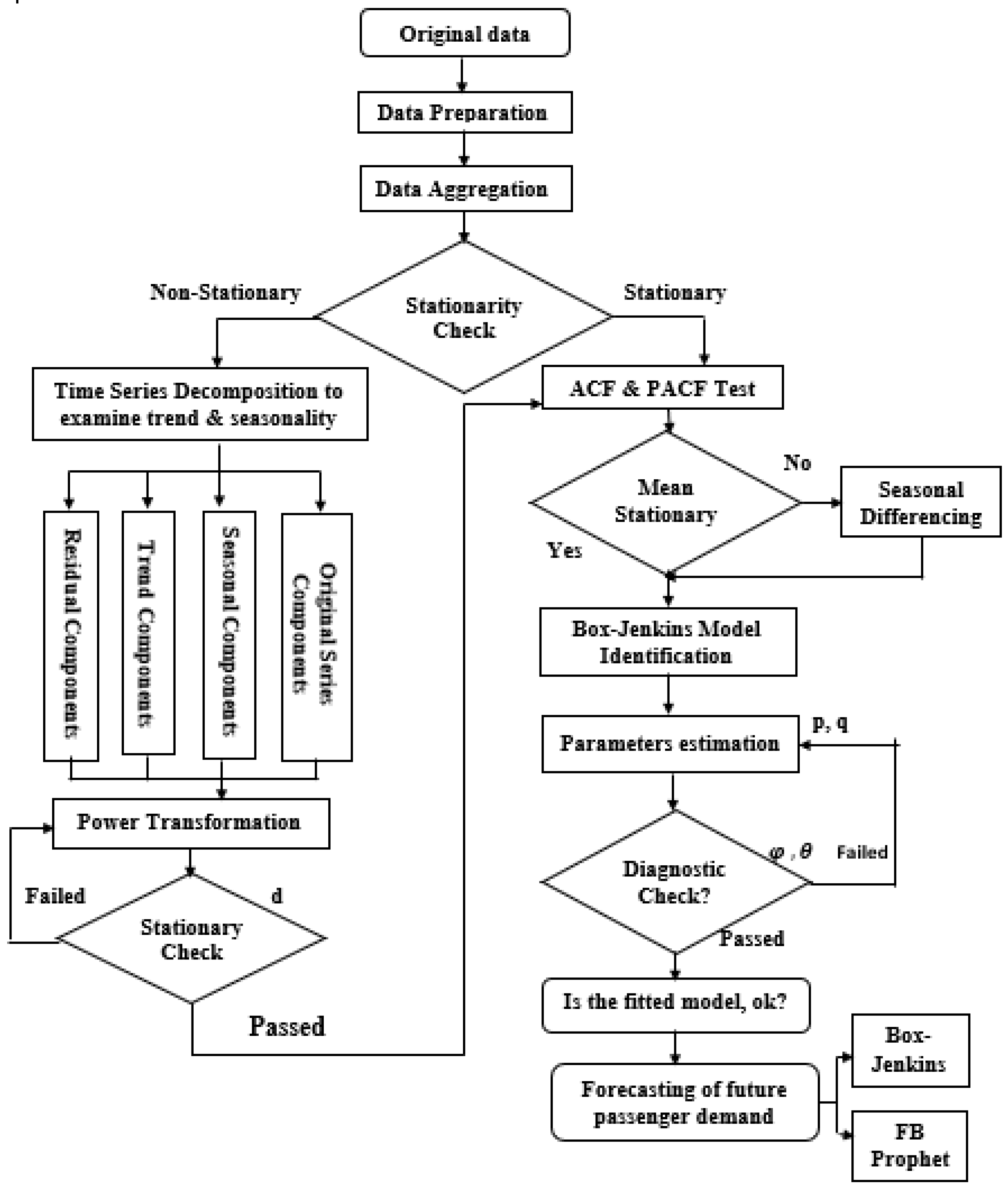
This section introduces the targeted URT station passenger demand data and the statistical techniques used. Time series forecasting is a technique used to achieve the goals and objectives of this study. The observed data used to predict future passenger demand is based on existing URT historical inbound data collected at specific intervals of time (one hour). Figure 8 shows the empirical passenger-data-based conceptual framework adopted for analyzing and modeling different time series.
3.1. Data Analysis
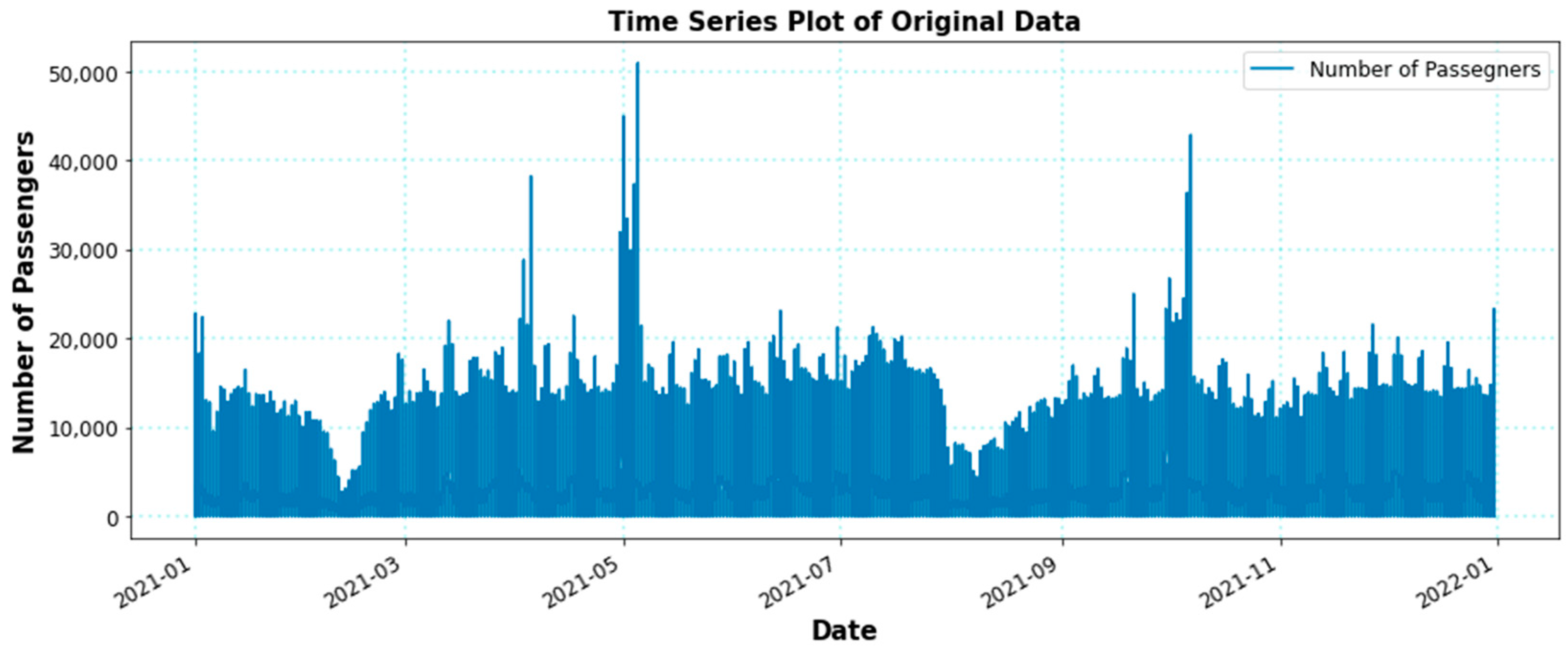
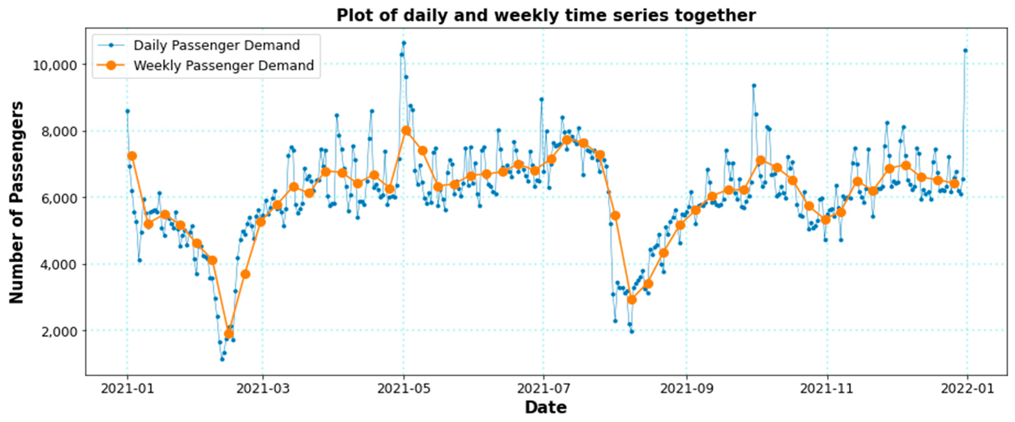
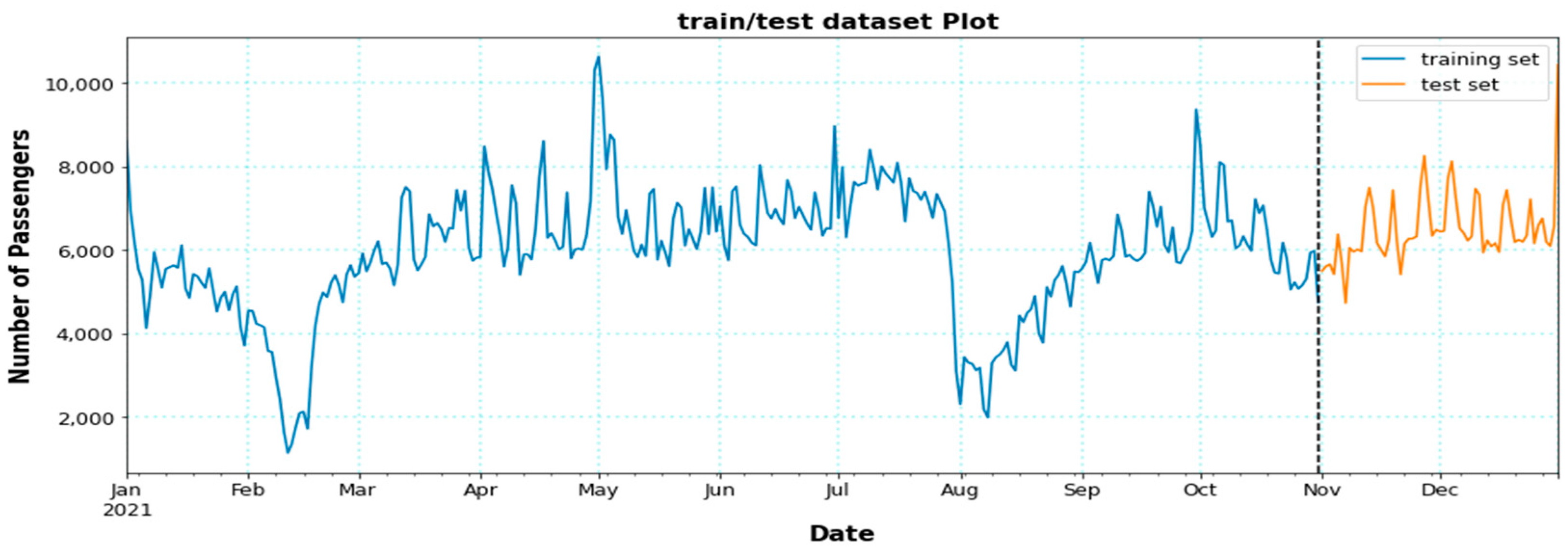
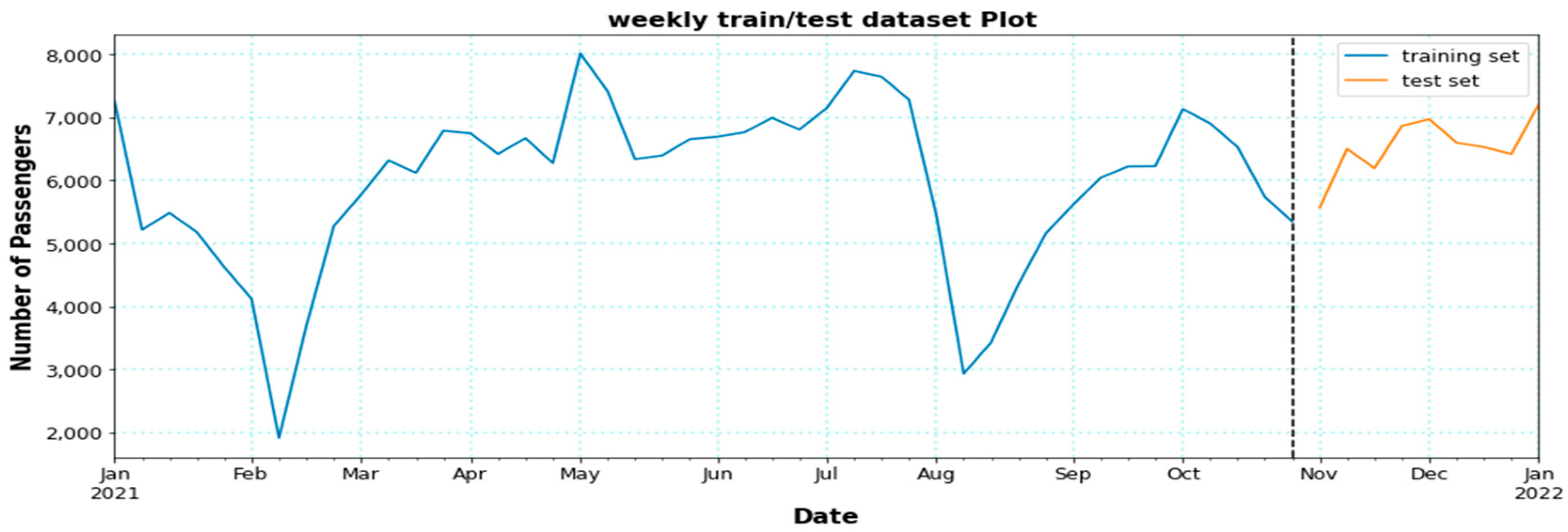
To construct the different time series models, namely daily and weekly, the data used are extracted from the smart card in the targeted URT station. The URT passenger demand data extracted depends on the corresponding entry station time by which the passengers entered the stations, as the outflow time of each passenger differs from station to station. The extracted historical passenger data covered the period from 1 January 2021 to 31 December 2021 and constituted 9125 observations aggregated in one hour. The time series data obtained were first plotted to observe the patterns and behaviors in the historical data over time. The time series plot shows the monthly numbers of passenger demand for arrival at this station against the date in months. Figure 1 displays the original inbound historical passenger demand. From the plot, we can observe that the passenger demand is far too dense to make much sense for the time series analysis. Therefore, to gain more insight into the original series, we aggregated the original time series data into daily and weekly time series (Figure 2), through which the forecast for the future passenger demand is made. After aggregating the data into the daily and weekly time series data, we further divided the daily and weekly data into a training dataset and a test dataset. The training and test dataset plots are displayed in Figure 3 and Figure 4. The train dataset consisting of data from 1 January 2021 to 31 October 2021 was used to develop the daily and weekly time series models and to calibrate the different models’ parameters. The test dataset consisting of data from 1 November 2021 to 31 December 2021 was used to validate the prediction computational efficiency and accuracy of different dependent models.
From Figure 1 and Figure 2, we can observe that the passenger demand values recorded in May, October, and April were the largest, which was due to Tomb-Sweeping Day, Labor Day, and National Day in China, respectively. In addition, there are festival activities, i.e., Chinese New Year (spring festival), Dragon boat festival, Mid-Autumn Festival, and New Year’s Day events, that contribute greatly to the rise in passenger demand values, while the observed decrease in passenger demand values in some months, i.e., February and August, are less caused by the impact of COVID-19, educational holidays, reduction in work trips, etc.
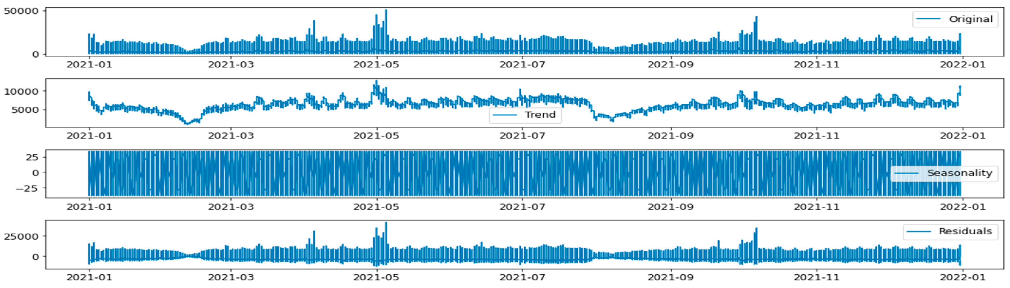
For a better in-depth understanding of the obtained historical passenger demand data, the original time series and the aggregated daily and weekly time series were further decomposed into separate components Figure 5, i.e., seasonal components , trend components , and residual components that a time series contained.
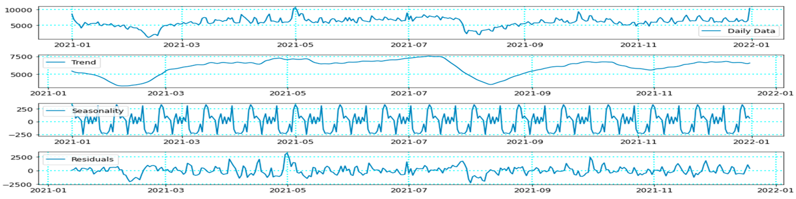
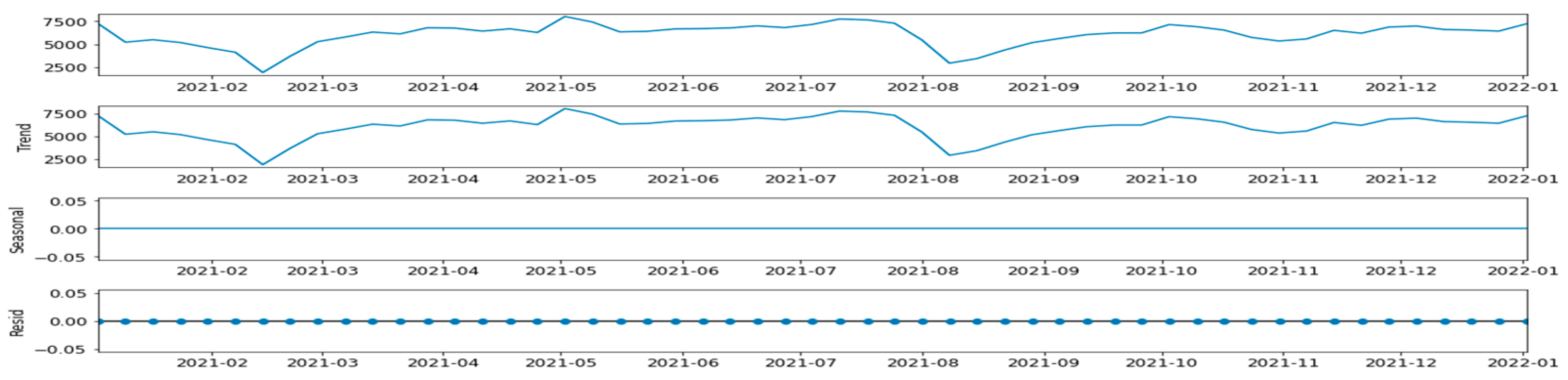
From the daily and weekly decomposed time series plot Figure 6 and Figure 7, we can observe that the daily time series seasonal decomposed box displayed repeated peaks, which signifies that the daily time series has seasonality. The trend component box indicates that the trend contributes greatly to the series and requires further time series transformation. The weekly time series seasonal decomposed box displayed no repeated peaks, which signified that the weekly time series does not have seasonality. The residual component box pattern shows the random nature of what is left of the original, daily, and weekly time series after accounting for seasonality and trend components.
3.2. Methodology
To forecast passenger demand for the targeted URT station, this study used the Box and Jenkins (1976) time series modeling technique and the Facebook Prophet time series modeling technique to build the daily and weekly time series model because of their stationarity nature, power, suitability, and flexibility to our dataset. The prediction models take into consideration the statistical theory and method as a foundation. Statistical software was used to analyze the daily and weekly time series characteristics and give a sense of how strong the underlying patterns such as trend , seasonality , mean, and variance are. The accuracy of Box–Jenkins and Facebook Prophet forecasting depends on the nature of the time series, which must first be made stationary. Stationarity tests were conducted using the augmented Dickey–Fuller test statistics (ADF) Equation (21) and the Kwiatkowski–Phillips–Schmidt–Shin test statistics (KPSS) Equation (22) for the daily and weekly time series forecasting models’ development before and after the series transformations. This study covered four major stages for the Box–Jenkins time series construction, such as identification of the time series models, estimation of the time series models’ parameters, diagnostic checking of the fitted models, and forecasting of the future station passenger demand. Figure 8 defines the model development stages explored in this study.
3.3. Box–Jenkins Forecasting Models
The introduction of the Box and Jenkins time series models and the AR, MA, ARMA, ARIMA [32], and SARIMA models were first illustrated.
3.3.1. Autoregressive (AR) (p) Models
Autoregressive models operate under the premise that the current passenger demand values of the series, , can simply be defined as a linear combination of p previous passenger demand values, , with a random error in the same series. An autoregression of the term (p) model AR (p) can be of the form:
where are the autoregressive coefficients or parameters of the model, are the actual values, is the residual error term of the series, c is the constant value derived from the mean of the series, and is the previous time series value of .
3.3.2. Moving Average (MA) (q) Model
The moving average of the term MA (q) is a model that measures only the direct effect of previous time lags on the current value. The MA of the term (q) model can be defined in the form:
where are the moving average coefficients or parameters of the model, are the actual values, is the residual error term of the series, and is the constant value derived from the mean of the series.
3.3.3. Autoregressive Moving Average (ARMA) (p, q) Model
The autoregressive moving average model, also called the ARMA (p, q) term, is developed by combining both the AR (p) terms and the MA (q) terms. The combination of Equations (4) and (6) gives the ARMA (p, q) model, defined as the following:
where is the prediction result of the ARMA (p, q) model, is the residual error term of the series, and are the coefficient or parameters of the model (p, q), c is the constant value derived from the mean of the series, is the previous time series value of , and is the previous residual error value.
3.3.4. Autoregressive Integrated Moving Average (ARIMA) (p, d, q) Model
The ARIMA model of the terms (p, d, q) adds lags of different series AR terms and lags of forecast error MA terms to the prediction. The general ARIMA model equation is defined as the following:
Differencing the series back one period gives the first-order difference and the general equation can be written as the following:
When the order of the differencing d (I) term is combined with the AR (p) term and MA (q) term model, a non-seasonal ARIMA model is found as defined in Equation (11):
where is the most current value in the time series, is the transformed series, is a set of uncorrected random shocks, is the backshift operator, is a non-seasonal AR operator, MA operator of order ‘p’, is a non-seasonal MA operator of order ‘q’, d is the differencing term, and c is the constant value derived from the series.
3.3.5. Seasonal Autoregressive Integrated Moving Average (SARIMA) Models
The SARIMA model is developed by including additional seasonal terms in the ARIMA Equation (11) models, defined as the following:
ARIMA
where m is the number of observations, B is the back shift operator, p and P, q and Q are the seasonal and non-seasonal AR and MA terms, respectively, used to determine the lagged values of and , and d and D define the order of seasonal and non-seasonal differencing, respectively.
3.3.6. Facebook Prophet (FB Prophet) Model
The Facebook Prophet is a powerful forecasting tool built by Facebook. Ref. [33] used a decomposable time series model with three main model components: trend, seasonality, and holidays, as defined in Equation (13):
where is the trend component, is the seasonality, is the holiday effects, is the error term, and is the prediction.
3.4. Forecasting Models Selection
Selecting a forecasting model depends mainly on the identified features and characteristics of the time series. The different time series data were analyzed through the application of statistical and mathematical models to make forecasts for future passenger values and provide appropriate information to the URT station authorities concerning strategic planning and decision-making. The choice of select Box–Jenkins and Facebook Prophet time series modeling techniques used in this analysis was due to the models’ designed abilities for univariate time series datasets. Both models are suitable for time series data with trend and seasonality effects and play a fundamental role in understanding how passenger demand values change over a period.
3.4.1. Box–Jenkins Model Selection Criterions
The Akaike information criterion (AIC), Bayesian information criterion (BIC), and maximum likelihood rule (ML) were considered the best model selection criteria among several tested candidate models in this study. The model with the least possible AIC value and BIC value information criteria is considered the most appropriate model. The AIC and BIC equations are written as in Equations (14) and (15):
where k is p + q estimated parameters in the model, while L = maximized likelihood value for the estimated model, n = number of observations (sample size), RSS = residual sum of squares of the estimated model, and is the error variance.
3.4.2. Performance Evaluation Index
The models’ results were compared by evaluating the performance of the best-fitted models using five model performance indexes to measure the model’s accuracy: mean squared error (MSE), mean absolute error (MAE), root mean square error (RMSE), root mean squared log error (RMSLE), and mean squared log error (MSLE). Mean square error (MSE) is the most commonly used error indicator in this study because of its usefulness in comparing different models; it shows the ability to predict the correct output. The RMSE is another error estimation used, which shows the error in the unit of actual and predicted data. Mean absolute error is used as the sum of absolute differences between the actual time series values and the forecasted values. The following performance evaluation equations were used in this study:
where = actual values, = forecasted values, and = number of observations.
Equation (16) measures the model goodness of fit and was also used as a model selection criterion. Equations (17) and (18) measure the average absolute and relative errors to determine how well the model can generate the time series data that are already available. Equations (19) and (20) are used to measure the ratio between actual values and forecasted values to penalize underestimated values more than overestimated values.
4. Results and Discussions
Each variable time series for evidence of stationarity and non-stationarity to be able to fit it into the proposed models was first examined.
4.1. Time Series Stationarity Test
Before the different time series (daily and weekly) models were built first, a stationarity test was conducted, as shown in Figure 8. The stationarity test in time series forecasting analysis indicates the constant nature of a series of statistical attributes, i.e., mean, variance, auto-correlation, etc., which implies the series exhibits low heteroskedasticity. In this study, the primary methods adopted to test the stationarity nature of the different series before and after the transformation among several other methods are the augmented Dickey–Fuller stationarity test (ADF) and Kwiatkowski–Phillips–Schmidt–Shin (KPSS) stationarity test. The regression equation given by Dickey–Fuller (1979) and KPSS for the stationarity test is written as in Equations (21) and (22):
where t = p + 1, p + 2…..., T, = intercept, = coefficient trend when present, = coefficient of the lagged dependent variable = p lags of with coefficient are added to account for the series correlation in the residuals, is the random walk, is the deterministic trend, is the stationary error term, and is the constant. If H0: = 0 means not stationary and the H0 is not rejected; also, if > 0, means stationary and the H0 is rejected, while the H1: means stationary. The ADF test statistics can be written as the following:
where = standard error for denotes estimates.
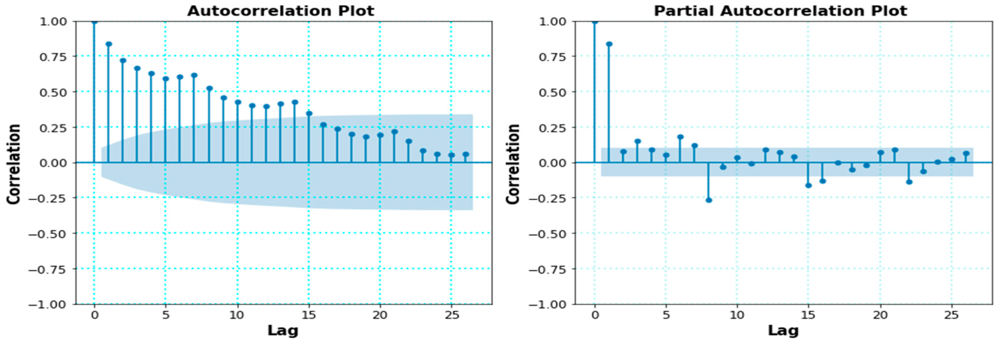
After the stationarity test, the next stage adopted is model identification. The model identification process was done by checking stationarity, trailing, and truncation features of the autocorrelation function ACF and partial autocorrelation function PACF to find the initial orders of seasonal and non-seasonal model hyperparameters, p, q, and P, Q, MA (q) terms and AR (p) terms. After the appropriate model has been identified by the number of significant spikes, the stability of the estimated parameters was examined to the period frame adopted in Figure 8. The goal is to generate statistically adequate representations of the different series and to select a model that has significant computing coefficients and a good fit. The ACF and PACF model behaviors are summarized in Table 1. The Ljung–Box (Q) test statistics model diagnostic checking was considered important to verify the adequacy of the good fit model. In addition, we repeated all these stages, which have a restatement condition if the model is invalid for the forecast. The Ljung–Box (Q) test equation can be defined as Equation (24):
where = estimated residual autocorrelation of the different series at lag k, m = number of lags.
4.2. Daily Time Series Model
The development of the daily forecasting model consists of daily passenger demand data extracted from the obtained original time series passenger data defined at the same period. In the daily passenger demand time series forecasting model development, the time series forecasting period is considered one day. By checking the ACF and PACF plots, Figure 9 and ADF stationarity test statistics, and KPSS stationarity test statistics conducted on the daily time series before transformation, results indicate that the daily time series ADF and KPSS shows no stationarity since the p-value of the series is 0.077616 > 0.05 for ADF and 0.024237 < 0.05 for KPSS. Therefore, to make the daily time series data that was not stationary become stationary, the auto-ARIMA modeling technique was used because of its power to automatically transform the data, output different candidates’ models, and suggest an appropriate model that satisfies the steps defined in Figure 8. Twenty-four hours was considered the daily time series frequency; this means that for the same period, existing passenger demand information can be utilized to forecast passenger demand data the next day.
The SARIMA model (p, d, q) (P, D, Q)m is considered appropriate for handling the daily transformed time series. After checking the different combinations of the candidates’ models, empirical results showed that the SARIMA (5, 1, 3) (1, 0, 0)24 model proved to have the best model performance among several tested candidates’ models for forecasting the future daily passenger demand for this targeted station line. The daily SARIMA (5, 1, 3) (1, 0, 0)24 model can be written as the following:
where is the prediction result of the daily SARIMA model, is the white noise of the daily series, and are the parameters of the daily model.
The daily time series model parameters, such as standard error, p-values results, etc., are shown in Table 2. Table 3 presents the fitting model’s performance evaluation index results for the daily series. From the observations made, the daily time series developed model accurately captures both the trend and seasonal fluctuations of the series and stipulates a suitable forecast for both weekdays and weekends. The developed SARIMA model (5, 1, 3) (1, 0, 0)24 proved to have good performance, especially on weekdays.
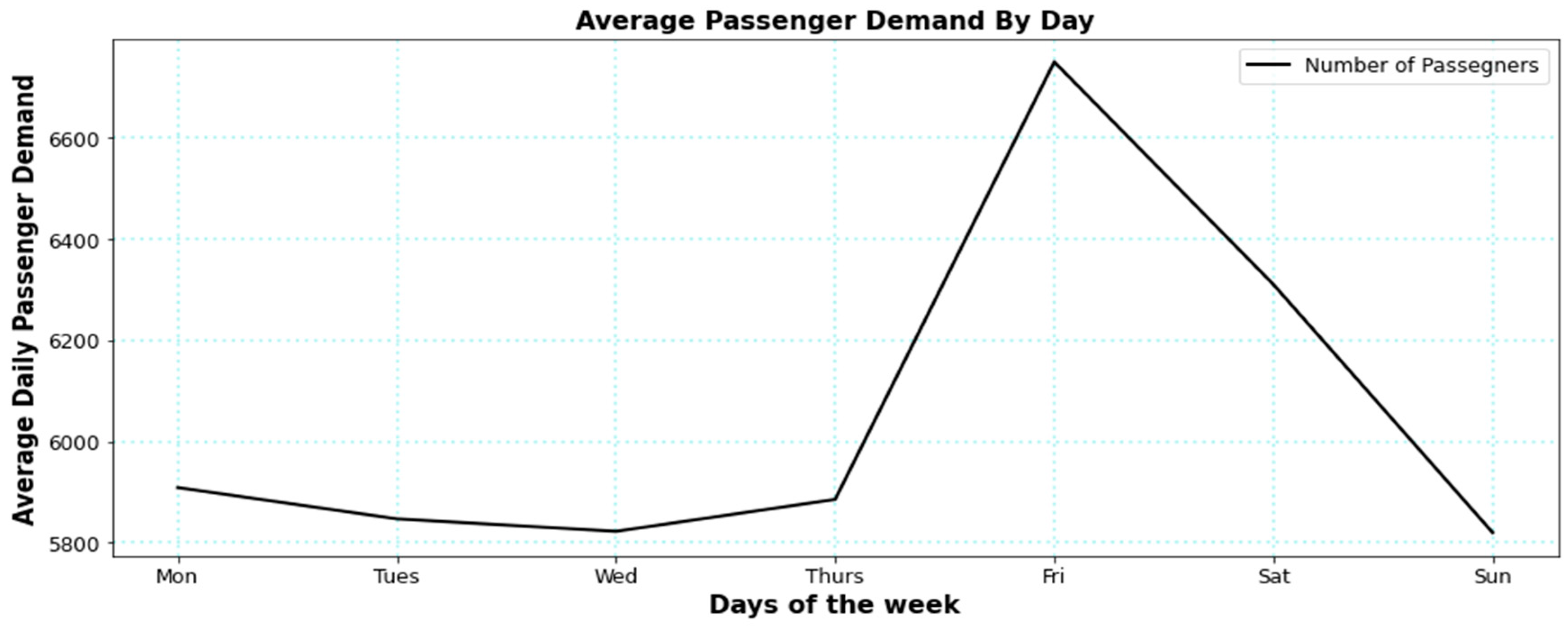
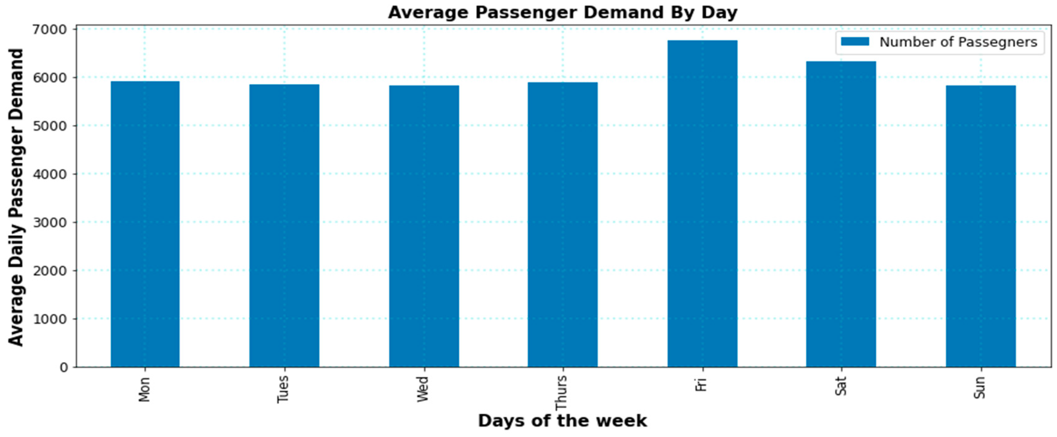
Figure 10 and Figure 11 displays the significant fluctuations between the weekday and weekend passenger demands for the targeted URT station. The figures show that passenger demand decreased starting on Monday and reached its lowest level on Tuesday, but passenger demand started to increase and found Friday to be the strongest day with maximum passenger demand. In addition, passenger demand tended to increase on weekends compared to working days because the URT station is linked to tourist attractions and commercial centers. The weakest day with the minimum passenger demand was Sunday.
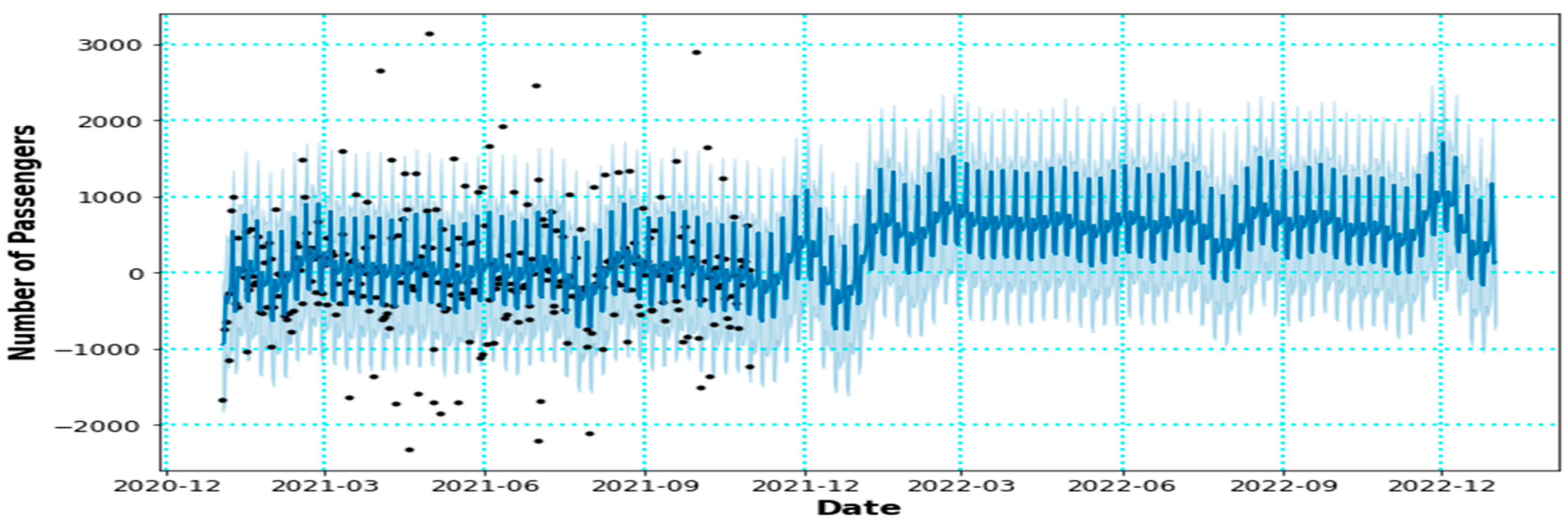
Figure 12 define the forecasted daily passenger demand for the additional 365 days using the Prophet model. As shown in the Figure 12, the black dots represent the actual training data, the blue lines represent time series model predictions, and the shaded area represents the 95% prediction interval (upper and lower).
4.3. Weekly Time Series Model
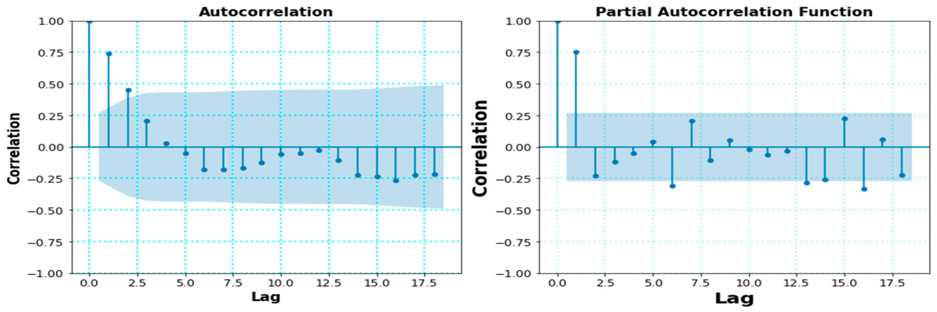
The development of the weekly passenger demand forecasting model consists of the weeks (i.e., traditional working weeks, festivals, and holidays) and passenger demand data extracted from the obtained inbound historical original time series data being defined at the same period on the same weekday. In the weekly series forecasting model development, the weekly time series forecasting period is considered one week. To build the weekly time series model, we first conducted a stationarity test using the ADF test statistics and KPPS test statistics. From the stationarity test statistic results, it was observed that the ADF test statistic −3.096067 is significantly smaller than the two critical values (i.e., critical values at 5% and 10%) with a p-value of 0.026846 < 0.05.05. In this case, we failed to accept the (Ho:) null hypothesis, and the (Ha:) alternative hypothesis is accepted. In addition, the KPSS test statistic is 0.087391, and the p-value 0.10000 > 0.05.05. In this case, we accepted the (Ho:) null hypothesis but failed to accept the (Ha:) alternative hypothesis. We concluded that the weekly time series data proved to be stationary with no power transformation and does not have a unit root. By checking the ACF and PACF plots, Figure 13. The ACF displays a tail-off exponentially while the PACF plot shuts off after different significant lags for different periods of the day. For the stationary time series, both the AR (p) and ARMA (p, q) models are considered suitable for modeling the weekly stationary series.
In modeling the AR (p) model, several candidate models of order p were first tested to select a suitable AR (p) model. The AIC, BIC, ML, and MSE model selection criteria were also used for the optimal model selection. The result proved that AR (2) is the appropriate model among several tested candidate models. In addition, model testing was employed in the ARMA (p, q) model considering different ARMA (p, q) model combinations. ARMA (2, 1) proved to be the best among the different tested candidate models. We further compared the two developed models, the AR (2) and ARMA (2, 1) models. The empirical results showed that the ARMA (2, 1) model was considered appropriate for modeling the weekly time series. The ARMA (2, 1) model can be written as the following:
where is the prediction result of the ARMA (p, q) model, is the white noise of the time series, and are the parameters of the model.
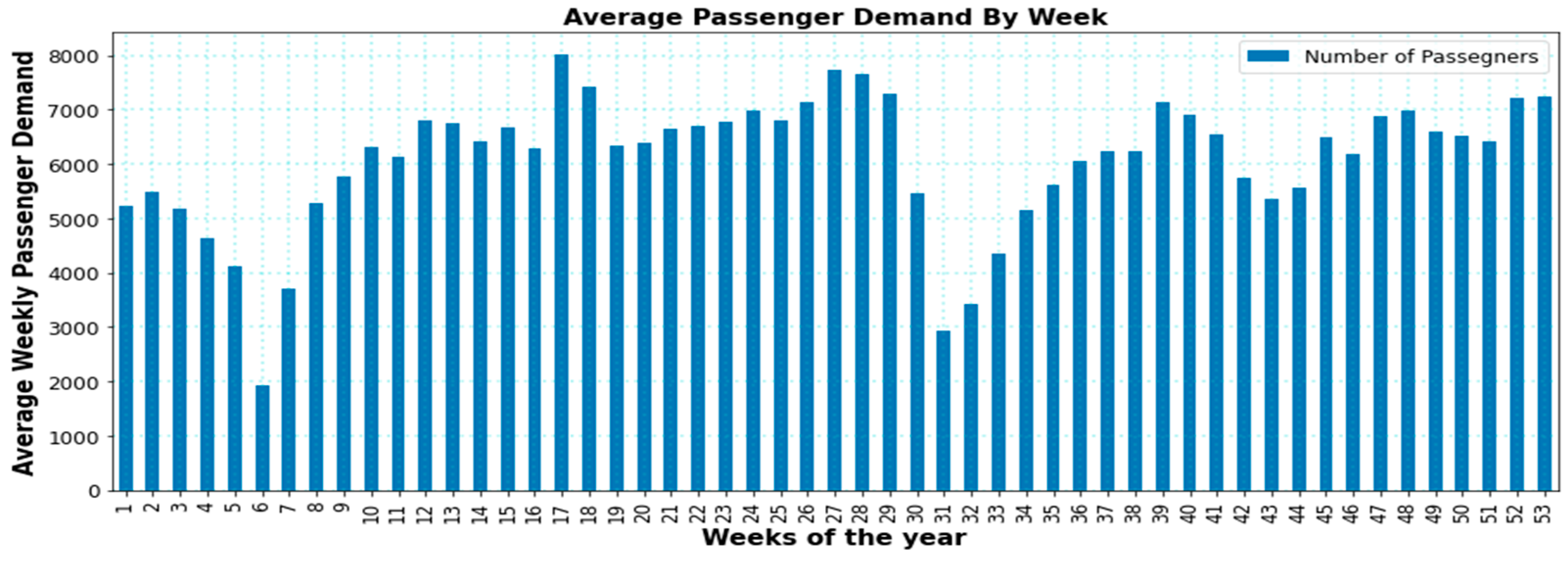
The weekly time series model parameters, such as standard error results, etc., are shown in Table 2. The fitting model’s performance evaluation index results for the weekly time series model are shown in Table 3. Based on the observations made, the weekly time series model accurately captures the trends of the weekly series and provides a suitable prediction for weeks of the year 2021 (Figure 14).
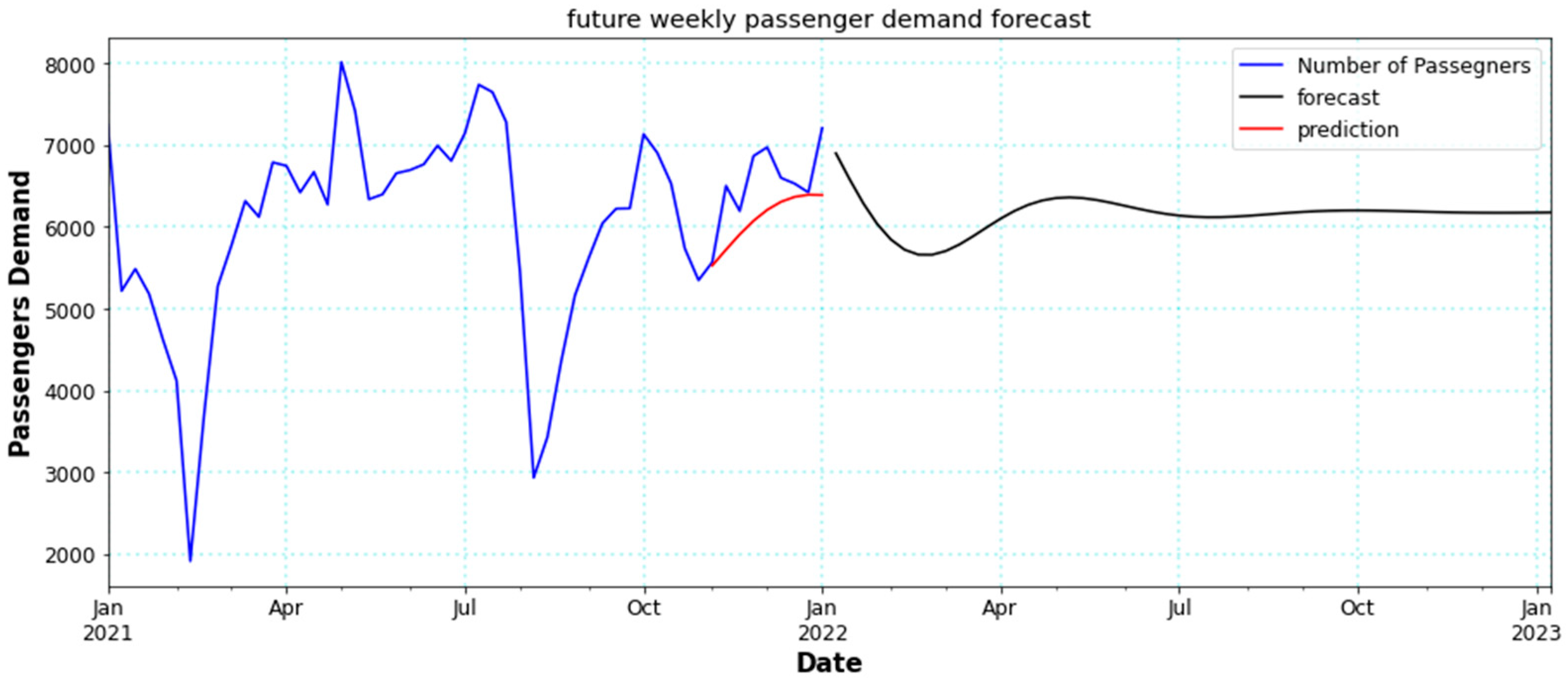
Figure 15 define the forecasted weekly passenger demand for the additional 53 weeks using the Box-Jenkins model. As indicated, the blue line represents the actual data, the red line shows the predicted time series, and the black line represents the post-future forecasted demand.
4.4. Forecasting with the Selected Model
The principal objective of developing the prediction model is to test whether it is capable of forecasting future passenger demand accurately or not for the same series. To build the model, the stages defined in Figure 8 were critically observed for the model development accuracy. The suitably selected models were used to create forecasts for the next 12 months of 2022. The forecasting performance, as well as the fitted model, is measured by evaluating the model performance index generated directly from Equations (16)–(20), the form of the model procedure.
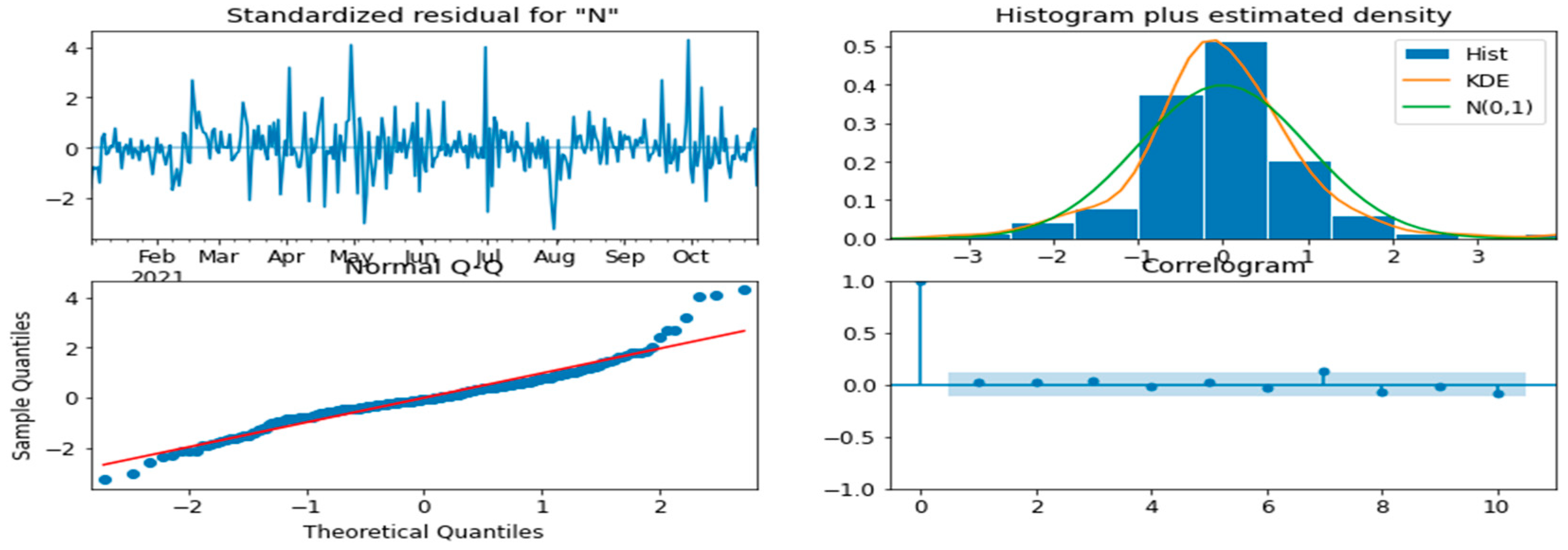
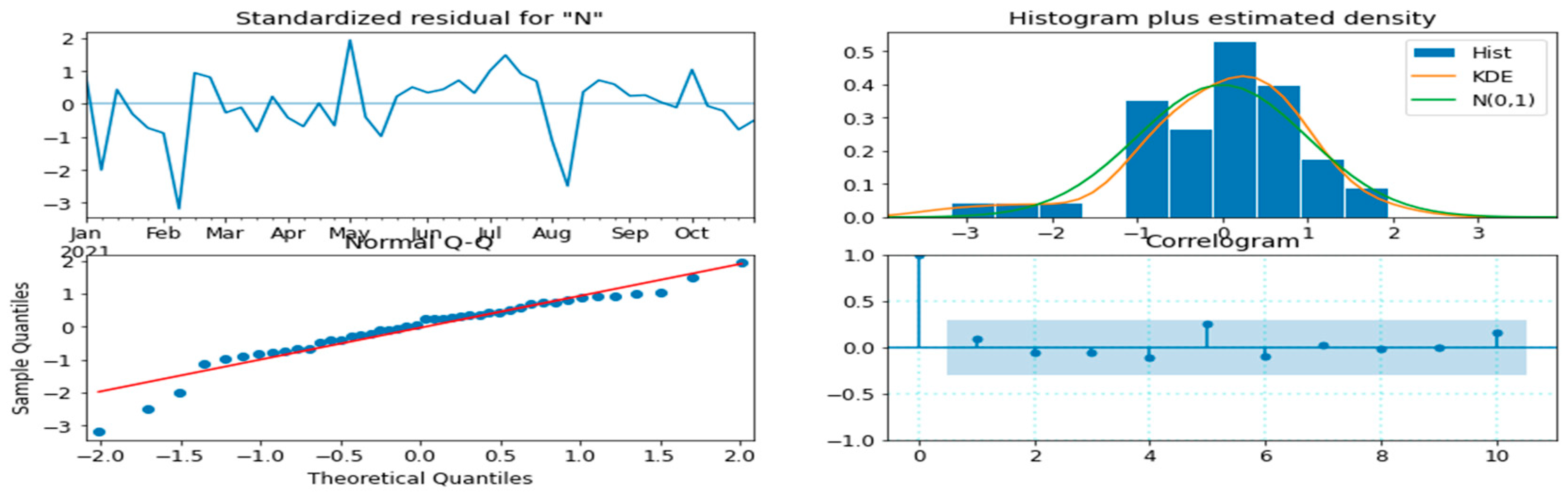
Figure 16 and Figure 17 show the model diagnostic plot for the developed daily and weekly time series models. The model residual quantile-quantile Q-Q plots and histogram followed a normal distribution. In addition, the model correlogram plot indicates that the residuals did not show any significant correlation.
5. Conclusions
The lack of studies in the context of URT passenger demand forecasts and the extent of including real-time data in forecasting models have propelled the analysis and development of daily and weekly URT passenger demand time series forecasting. The studied results are recapitulated as follows:
1. This study used the actual 365 days of historical inbound-passenger-demand data collected from the targeted URT station to construct the different time series forecasting models based on the Box–Jenkins and FB Prophet forecasting models’ approach applied to predict the post-daily and weekly passenger demand of the same station being studied and to examine the forecasting performance of the algorithms used, based on the context of aggregated URT-passenger-demand data. These predictions are more productive for URT authorities for operational scheduling.
2. After the correlation, stationarity and periodicity analysis of the passenger demand characteristics were conducted to determine the appropriate forecasting models. The daily and weekly passenger demand forecasting method of URT is proposed using a time series algorithm, and the effectiveness of the method is examined through the display of prediction results and comparative analysis. The corresponding forecasting models, the SARIMA, ARMA, and FB Prophet models, were developed to capture different characteristics and features of the series.
3. We investigated the different models’ forecast performance accuracy of the different constructed time series models and chose the optimal models. Based on the algorithms used, the daily and weekly passenger demand forecasting model of URT was constructed, with MAE, RMSE, and MSE as the performance evaluation indicators of the model, and the parameters of each model were optimized and validated, and the optimal prediction results of each model were output.
4. To achieve better forecast results, we experimented with several candidate models for the different Box–Jenkins time series (daily and weekly) models, as shown in Table 4. For each developed candidate model, we estimated the parameters thereafter. Using the model selection criteria explored, it was observed that the ARMA (2, 1) model for the weekly time series forecast and the SARIMA (5, 1, 3) (1, 0, 0)24 model for the daily time series forecast satisfied the selection conditions as the suitable models. Implying that the choice of ARMA (2, 1) and SARIMA (5, 1, 3) (1, 0, 0)24 are appropriate and ideal, we further compared the Box–Jenkins model with the FB Prophet model as in Table 3. As a next step, we made forecasts for the next 12 months of 2022. Finally, the prediction results show that the passenger demand for this targeted URT station line has shown a trend toward an increase and decrease in passenger demand for both daily and weekly time series forecasts. In addition, because of the fluctuation effect of demand on weekdays and weekends, heteroskedasticity was considered.
Future lines of study include improving the performance and practicality of the study by considering predicting weekends, working weeks before the summer holidays, holidays, and some sudden passenger demand, making the forecast range more comprehensive. In this study, only inbound passenger demand at the targeted URT station was considered. In the future, we can predict the regional passenger demand at the station and the cross-sectional passenger demand of the line and then optimize the URT operation organization. In the forecasting process of this study, the impact factors such as passenger transfers, access to new lines in the network, weather changes, and other means of transport are not considered. To further improve the accuracy of the forecast, comprehensive considerations can be carried out in the future steps of the study to enhance the persuasiveness of the study. Finally, this study has proved that researchers can achieve impressive increases in forecasting accuracy through the application of Facebook Prophet time series modeling techniques because of the model’s designed ability to capture yearly, weekly, and daily seasonality and trend components in the time series. The comparative evaluation as in Table 3 of the Box–Jenkins against Facebook Prophet time series models has indicated the overall superiority of the Facebook Prophet in modeling the daily URT forecasts of passenger demand values. The Box–Jenkins model shows superiority over Facebook Prophet in modeling the weekly time series.
Author Contributions
W.C. took responsibility for data collection, investigation, review and editing of manuscript, resources, and supervision. D.D.C. designed the ideas of the study, methodology, writing-original draft preparation, writing-review and editing, software design, formal analysis, and data curation. Visualization and Validation were done by W.C. and D.D.C. All authors have read and agreed to the published version of the manuscript.
Funding
This research is supported by the open funding from the Rail Data Research and Application Key Laboratory of Hunan Province at Central South University (Grant No. 502401004), and partly supported by the Science Progress and Innovation Program of DOT of Hunan Province (Grant No. 201949).
Data Availability Statement
The data presented in this study are available on request from the corresponding author. The data are not publicly available due to city government and urban rail transit policies.
Acknowledgments
The authors would like to thank the urban rail transit (URT) company for the data collection.
Conflicts of Interest
The authors declare no conflict of interest.
References
- Ahmed, M.S.; Cook, A.R. Analysis of Freeway Traffic Time-Series Data by Using Box-Jenkins Techniques; The National Academies of Sciences, Engineering, and Medicine: Washington, DC, USA, 1979. [Google Scholar]
- Ahmed, S.A. On the Estimation of Traffic Occupancy with Application to Freeway Incident Detection. IFAC Proc. Vol. 1982, 15, 819–823. [Google Scholar] [CrossRef]
- Bai, L.; Yao, L.; Kanhere, S.S.; Yang, Z.; Chu, J.; Wang, X. Passenger Demand Forecasting with Multi-Task Convolutional Recurrent Neural Networks. In Advances in Knowledge Discovery and Data Mining; Yang, Q., Zhou, Z.-H., Gong, Z., Zhang, M.-L., Huang, S.J., Eds.; Springer International Publishing: Cham, Switzerland, 2019; Volume 11440, pp. 29–42. ISBN 978-3-030-16144-6. [Google Scholar]
- Chen, C.F.; Chang, Y.H.; Chang, Y.W. Seasonal ARIMA forecasting of inbound air travel arrivals to Taiwan. Transportmetrica 2009, 5, 125–140. [Google Scholar] [CrossRef]
- Chikkakrishna, N.K.; Hardik, C.; Deepika, K.; Sparsha, N. Short-Term Traffic Prediction Using SARIMA and FbPROPHET. In Proceedings of the 2019 IEEE 16th India Council International Conference (INDICON), Rajkot, India, 13–15 December 2019; pp. 1–4. [Google Scholar]
- Fang, Z.; Cheng, Q.; Jia, R.; Liu, Z. Urban Rail Transit Demand Analysis and Prediction: A Review of Recent Studies. In Intelligent Interactive Multimedia Systems and Services; De Pietro, G., Gallo, L., Howlett, R.J., Jain, L.C., Vlacic, L., Eds.; Springer International Publishing: Cham, Switzerland, 2019; Volume 98, pp. 300–309. ISBN 978-3-319-92230-0. [Google Scholar]
- Fathi, O. Time series forecasting using a hybrid ARIMA and LSTM model. Velv. Consult. 2019, 1–7. [Google Scholar]
- Hansen, J.V.; McDonald, J.B.; Nelson, R.D. Time Series Prediction with Genetic-Algorithm Designed Neural Networks: An Empirical Comparison with Modern Statistical Models. Comput. Intell. 1999, 15, 171–184. [Google Scholar] [CrossRef]
- Harvey, A.C.; Peters, S. Estimation Procedures for Structural Time Series Models. J. Forecast. 1990, 9, 21. [Google Scholar] [CrossRef]
- Hong, W.C.; Dong, Y.; Zheng, F.; Lai, C.Y. Forecasting urban traffic flow by SVR with continuous ACO. Appl. Math. Model. 2011, 35, 1282–1291. [Google Scholar] [CrossRef]
- Karlaftis, M.G.; Vlahogianni, E.I. Statistical methods versus neural networks in transportation research: Differences, similarities and some insights. Transp. Res. Part C Emerg. Technol. 2011, 19, 387–399. [Google Scholar] [CrossRef]
- Kumar, S.V.; Vanajakshi, L. Short-term traffic flow prediction using seasonal ARIMA model with limited input data. Eur. Transp. Res. Rev. 2015, 7, 21. [Google Scholar] [CrossRef] [Green Version]
- Lee, S.; Fambro, D.B. Application of Subset Autoregressive Integrated Moving Average Model for Short-Term Freeway Traffic Volume Forecasting. Transp. Res. Rec. 1999, 1678, 179–188. [Google Scholar] [CrossRef]
- Li, W.; Sui, L.; Zhou, M.; Dong, H. Short-term passenger flow forecast for urban rail transit based on multi-source data. EURASIP J. Wirel. Commun. Netw. 2021, 2021, 9. [Google Scholar] [CrossRef]
- Milenković, M.; Švadlenka, L.; Melichar, V.; Bojović, N.; Avramović, Z. SARIMA modelling approach for railway passenger flow forecasting. Transport 2016, 33, 1113–1120. [Google Scholar] [CrossRef]
- Montgomery, D.C.; Jennings, C.L.; Kulahci, M. Introduction to Time Series Analysis and Forecasting; Wiley-Interscience: Hoboken, NJ, USA, 2008; ISBN 978-0-471-65397-4. [Google Scholar]
- Oh, S.; Byon, Y.J.; Jang, K.; Yeo, H. Short-term Travel-time Prediction on Highway: A Review of the Data-driven Approach. Transp. Rev. 2015, 35, 4–32. [Google Scholar] [CrossRef]
- Rabbani, M.B.A.; Musarat, M.A.; Alaloul, W.S.; Rabbani, M.S.; Maqsoom, A.; Ayub, S.; Bukhari, H.; Altaf, M. A Comparison Between Seasonal Autoregressive Integrated Moving Average (SARIMA) and Exponential Smoothing (ES) Based on Time Series Model for Forecasting Road Accidents. Arab. J. Sci. Eng. 2021, 46, 11113–11138. [Google Scholar] [CrossRef]
- Raza, A.; Zhong, M. Lane-based short-term urban traffic forecasting with GA designed ANN and LWR models. Transp. Res. Procedia 2017, 25, 1430–1443. [Google Scholar] [CrossRef]
- Smith, B.L.; Williams, B.M.; Keith Oswald, R. Comparison of parametric and nonparametric models for traffic flow forecasting. Transp. Res. Part C Emerg. Technol. 2002, 10, 303–321. [Google Scholar] [CrossRef]
- Song, H.; Tang, T.; Li, C.; Ding, Y. Short Time Forecasting of Rail Transit Passenger Volume. In The 2nd International Symposium on Rail Transit Comprehensive Development (ISRTCD) Proceedings; Xia, H., Zhang, Y., Eds.; Springer: Berlin/Heidelberg, Germany, 2014; pp. 121–130. ISBN 978-3-642-37588-0. [Google Scholar]
- Van Der Voort, M.; Dougherty, M.; Watson, S. Combining Kohonen maps with Arima time series models to forecast traffic flow. Transp. Res. Part C Emerg. Technol. 1996, 4, 307–318. [Google Scholar] [CrossRef] [Green Version]
- Vlahogianni, E.I.; Golias, J.C.; Karlaftis, M.G. Short-term traffic forecasting: Overview of objectives and methods. Transp. Rev. 2004, 24, 533–557. [Google Scholar] [CrossRef]
- Wang, X.; Zhang, N.; Zhang, Y.; Shi, Z. Forecasting of Short-Term Metro Ridership with Support Vector Machine Online Model. J. Adv. Transp. 2018, 2018, 3189238. [Google Scholar] [CrossRef]
- Wei, Y.; Chen, M.C. Forecasting the short-term metro passenger flow with empirical mode decomposition and neural networks. Transp. Res. Part C Emerg. Technol. 2012, 21, 148–162. [Google Scholar] [CrossRef]
- Williams, B.M. Multivariate Vehicular Traffic Flow Prediction: Evaluation of ARIMAX Modeling. Transp. Res. Rec. 2001, 1776, 194–200. [Google Scholar] [CrossRef]
- Williams, B.M.; Durvasula, P.K.; Brown, D.E. Urban Freeway Traffic Flow Prediction: Application of Seasonal Autoregressive Integrated Moving Average and Exponential Smoothing Models. Transp. Res. Rec. 1998, 1644, 132–141. [Google Scholar] [CrossRef]
- Williams, B.M.; Hoel, L.A. Modeling and Forecasting Vehicular Traffic Flow as a Seasonal ARIMA Process: Theoretical Basis and Empirical Results. J. Transp. Eng. 2003, 129, 664–672. [Google Scholar] [CrossRef] [Green Version]
- Yang, J.; Han, L.D.; Freeze, P.B.; Chin, S.M.; Hwang, H.L. Short-Term Freeway Speed Profiling Based on Longitudinal Spatiotemporal Dynamics. Transp. Res. Rec. J. Transp. Res. Board 2014, 2467, 62–72. [Google Scholar] [CrossRef]
- Zhang, J.; Chen, F.; Guo, Y.; Li, X. Multi-graph convolutional network for short-term passenger flow forecasting in urban rail transit. IET Intell. Transp. Syst. 2020, 14, 1210–1217. [Google Scholar] [CrossRef]
- Zhang, M. Time Series: Autoregressive models AR, MA, ARMA, ARIMA; University of Pittsburgh: Pittsburgh, PA, USA, 2018. [Google Scholar]
- Zhao, Y.; Ma, Z.; Yang, Y.; Jiang, W.; Jiang, X. Short-Term Passenger Flow Prediction with Decomposition in Urban Railway Systems. IEEE Access 2020, 8, 107876–107886. [Google Scholar] [CrossRef]
- Zuva, T.; Ngwira, S.M.; Zuva, K.; Ojo, S.O. Effectiveness of Non-Parametric Techniques in Image Retrieval. In Proceedings of the 2014 World Symposium on Computer Applications & Research (WSCAR), Sousse, Tunisia, 18–20 January 2014. [Google Scholar]
Figure 1.
The original series’ plot.

Figure 2.
Combined plots of daily and weekly time series data.

Figure 3.
Daily training and testing datasets.

Figure 4.
Weekly training and test datasets.

Figure 5.
The decomposed plot of the original series.

Figure 6.
The daily series decomposed plot.

Figure 7.
The weekly series decomposed plot.

Figure 8.
The framework process covered for the construction and selection of the best model.

Figure 9.
The daily time series AFC and PACF plot before the series transformation.

Figure 10.
The wide gap between weekdays and weekends.

Figure 11.
Bar plot of Figure 10.
Figure 11.
Bar plot of Figure 10.

Figure 12.
The plot of actual vs. prediction using the prophet model.

Figure 13.
The weekly time series ACF and PACF plot at no transformation.

Figure 14.
Passenger demand by weeks of the year.

Figure 15.
Weekly passenger demand plot with forecasted values using the Box–Jenkins model.

Figure 16.
Daily time series residual plot.

Figure 17.
Weekly time series residual plot.


Table 1.
ACF and PACF model behavior.
| Categories | AR (p) | MA (q) | ARMA (p, q) |
|---|---|---|---|
| ACF | Tails off exponentially | Shuts off after lag q | Tails off exponentially |
| PACF | Shuts off after lag p | Tails off exponentially | Tails off exponentially |
Table 2.
Parameters of daily and weekly time series model for the Box–Jenkins.
| Model | Parameters | Coefficient | Std Error | z | p-Value | ||
|---|---|---|---|---|---|---|---|
| Daily Time Series Model | SARIMA (5, 1, 3) (1, 0, 0)24 | −0.02 | 0.17 | −0.12 | 0.91 | ||
| −0.81 | 0.11 | −7.06 | 0.00 | *** | |||
| 0.25 | 0.20 | 1.21 | 0.23 | ||||
| −0.08 | 0.07 | −1.23 | 0.22 | ||||
| −0.18 | 0.07 | −2.70 | 0.01 | *** | |||
| −0.17 | 0.17 | −0.99 | 0.32 | ||||
| 0.72 | 0.07 | 9.83 | 0.00 | *** | |||
| −0.56 | 0.16 | −3.46 | 0.00 | *** | |||
| AR.S. L24 | −0.14 | 0.07 | −1.89 | 0.06 | |||
| Weekly Time Series Model | AR (2) | 1.01 | 0.15 | 6.76 | 0.00 | *** | |
| −0.32 | 0.15 | −2.19 | 0.03 | *** | |||
| ARMA (2, 1) | 1.72 | 0.08 | 20.62 | 0.00 | *** | ||
| −0.81 | 0.09 | −9.37 | 0.00 | *** | |||
| −0.99 | 0.07 | −14.86 | 0.00 | *** | |||
Where *** signified a 5% level of significance.
Table 3.
Prediction performance of the different models SARIMA vs. Prophet models.
| Model | RMSE | MAE | MSLE | RMSLE |
|---|---|---|---|---|
| SARIMA (5, 1, 3) (1, 0, 0) | 1346.908 | 1109.53 | 0.043 | 0.208 |
| AR (2) | 719.674 | 643.19 | 0.013 | 0.113 |
| AR (3) | 719.528 | 645.18 | 0.013 | 0.113 |
| AR (6) | 780.641 | 666.30 | 0.015 | 0.124 |
| ARMA (2, 1) | 469.818 | 360.54 | 0.005 | 0.072 |
| ARMA (0, 3) | 676.571 | 580.62 | 0.011 | 0.105 |
| ARMA (1, 3) | 680.431 | 588.11 | 0.011 | 0.106 |
| Facebook Prophet Time Series Model | ||||
| Daily Time Series | RMSE | MSE | MAE | |
| Baseline Model | 634.47 | 402,553.33 | 421.74 | |
| Baseline Model with Seasonality | 683.96 | 467,800.51 | 475.55 | |
| Weekly Time Series | ||||
| Baseline Model | 844.39 | 712,998.67 | 730.00 | |
| Baseline Model with Seasonality | 6304.62 | 38,497,293.63 | 6161.41 | |
Table 4.
Performance evaluation of different models for Box–Jenkins.
| SARIMA (p, d, q) (P, D, Q)m Models | Daily Time Series | |||
|---|---|---|---|---|
| AIC | BIC | MSE | Log-Likelihood | |
| SARIMA (5, 1, 3) (1, 0, 0)24 | 4828.786 | 4865.923 | 1,814,162.356 | −2404.393 |
| Weekly Time Series | ||||
| AR (2) | 722.86 | 729.99 | 517,930.55 | −357.43 |
| AR (3) | 724.73 | 733.65 | 517,720.89 | −357.36 |
| AR (6) | 723.74 | 738.01 | 609,400.54 | −353.87 |
| ARMA (2, 1) | 722.28 | 731.20 | 220,728.66 | −356.14 |
| ARMA (0, 3) | 720.32 | 729.25 | 457,775.37 | −355.16 |
| ARMA (1, 3) | 721.985 | 732.690 | 462,986.61 | −354.99 |
Publisher’s Note: MDPI stays neutral with regard to jurisdictional claims in published maps and institutional affiliations. |
© 2022 by the authors. Licensee MDPI, Basel, Switzerland. This article is an open access article distributed under the terms and conditions of the Creative Commons Attribution (CC BY) license (https://creativecommons.org/licenses/by/4.0/).
Share and Cite
MDPI and ACS Style
Chuwang, D.D.; Chen, W. Forecasting Daily and Weekly Passenger Demand for Urban Rail Transit Stations Based on a Time Series Model Approach. Forecasting 2022, 4, 904-924. https://0-doi-org.brum.beds.ac.uk/10.3390/forecast4040049
AMA Style
Chuwang DD, Chen W. Forecasting Daily and Weekly Passenger Demand for Urban Rail Transit Stations Based on a Time Series Model Approach. Forecasting. 2022; 4(4):904-924. https://0-doi-org.brum.beds.ac.uk/10.3390/forecast4040049
Chicago/Turabian StyleChuwang, Dung David, and Weiya Chen. 2022. "Forecasting Daily and Weekly Passenger Demand for Urban Rail Transit Stations Based on a Time Series Model Approach" Forecasting 4, no. 4: 904-924. https://0-doi-org.brum.beds.ac.uk/10.3390/forecast4040049