Spherical One-Way Wave Equation

Abstract

The coordinate-free one-way wave equation is transferred in spherical coordinates. Therefore it is necessary to achieve consistency between $gradient$, $divergence$ and $Laplace$ operators and to establish, beside the conventional radial Nabla operator $\mathrm{\partial }\mathrm{\Phi }/\mathrm{\partial }r$, a new variant $\mathrm{\partial }r\mathrm{\Phi }/r\mathrm{\partial }r$. The two Nabla operator variants differ in the near field term $\mathrm{\Phi }/r$ whereas in the far field $r\gg 0$ there is asymptotic approximation. Surprisingly, the more complicated gradient $\mathrm{\partial }r\mathrm{\Phi }/r\mathrm{\partial }r$ results in unexpected simplifications for – and only for – spherical waves with the $1/r$ amplitude decrease. Thus the calculation always remains elementary without the wattless imaginary near fields, and the spherical Bessel functions are obsolete.

1. Introduction

Seismics, sonar, sodar, room and machine acoustics, ultrasound diagnosis and tomography depend on the calculation of sound paths in solid, liquid or gaseous media with heterogenous physical properties and complex geometry. Calculations are based on the well-known equations of motion listed by Augustin-Louis Cauchy 200 years ago:

In a continuum with stationary cartesian coordinates $\mathit{x}=\{x{\mathit{e}}_{\mathit{x}},y{\mathit{e}}_{\mathit{y}},z{\mathit{e}}_{\mathit{z}}\}$ and modulus of elasticity E [Pa] a vectorial, elastic deflection $\mathit{s}=\mathit{s}(\mathit{x},t)$ [m] causes the stress tensor $\mathit{T}=E\mathbf{\nabla }\mathit{s}$ [Pa]. The local equilibrium of the tension force $div\mathit{T}=divE\mathbf{\nabla }\mathit{s}=E\Delta \mathit{s}$ [N/m${}^3$] due to stress tensor $\mathit{T}$ and the inertial force $\rho \ddot{\mathit{s}}$ [N/m${}^3$] caused by the local acceleration $\ddot{\mathit{s}}={\mathrm{\partial }}^2\mathit{s}/\mathrm{\partial }{t}^2$ [m/s${}^2$] can be written as

$$\rho \ddot{\mathit{s}}-E\Delta \mathit{s}=\mathbf{0}$$

(1)

By merging density $\rho$ [kg/m${}^3$] and elasticity module E sound velocity $c=\sqrt{E/\rho }$ [m/s] results and the governing wave equation for a homogeneous medium follows:

$$\ddot{\mathit{s}}-c^2\Delta \mathit{s}=\mathbf{0}$$

(2)

The partial differential equation (PDE) of the 2nd order (2) delivers two mutually independent solutions. From the quadratic velocity term $c^2={(+c)}^2={(-c)}^2$ can be seen that there are two waves travelling in opposite directions $+c$ and $-c$, hence results the designation “Two-way wave equation”. Regardless of this ambiguity, irregular phantom effects occur in numerical seismic FE or FD wave calculations.

To eleminate these unwanted effects a great number of auxiliary equations have been developed, but no specific approach has been able to prevail. Because of the economic importance of the “One-Way”/“Two-Way” problem there also exist numerous patent applications beside the scientific literature [1,2,3].

Due to the above mentioned difficulties the conventionally used equilibrium of forces was – initially hypothetically – replaced by an impulse equilibrium, i.e., more precisely by an impulse flow equilibrium [4,5]. Force and impulse are related and differ in one level of differentiation. Therefore, the unit of the impulse $Huygens$ [Hy = mkg/s = mass multiplied by velocity] was used. For a particle velocity $\dot{\mathit{s}}=\mathrm{\partial }\mathit{s}/\mathrm{\partial }t$ [m/s] the local specific impulse $\rho \dot{\mathit{s}}$ [Hy/m${}^3$] follows. If velocity $\dot{\mathit{s}}$ propagates with the vectorial wave velocity $\mathit{c}$, the dyadic product $\rho \mathit{c}\dot{\mathit{s}}$ results in a kinetic impulse flow of the dimension [Hy/sm${}^2$], i.e., $Huygens$ [Hy] per time and per area. On the other hand, an elastic deformation $\mathbf{\nabla }\mathit{s}$ induces the potential impulse flow $\mathbf{T}=E\mathbf{\nabla }\mathit{s}$ [Hy/sm${}^2$]. Wheras the Cauchy force equilibrium is applied to an infinitesimal volume element $dV=dxdydz$, the equilibrium of kinetic and potential impulse flow in each field point $\mathit{x}$ results in

$$\rho \mathit{c}\dot{\mathit{s}}-E\mathbf{\nabla }\mathit{s}=0$$

(3)

This tensor equation being scalarly multiplied by the vectorial wave velocity $\mathit{c}$ leads together with the known relationship $E=\rho c^2$ to a vectorial partial differential equation (PDE) of the 1st order respectively vectorial “One-Way wave equation”

$$\dot{\mathit{s}}-\mathit{c}·\mathbf{\nabla }\mathit{s}=0$$

(4)

Representing the equivalent to the force based 2nd order PDE wave Equation (2). Mathematically, the 1st order PDE is much easier than the 2nd order PDE with the higher differentiation level. Also the wave propagation direction is determined. Force and impulse concept are compared below in

Table 1. Comparison of force based Two-Way Wave Equation and impulse based One-Way Wave Equation in an unlimited, elastic 3D contiuum without boundary effects. For simplicity and clarification linearity, homogeneity, isotropy and losslessness are assumed; $\mathit{s}$[m] = elastic displacement, $\dot{\mathit{s}}=\mathrm{\partial }\mathit{s}/\mathrm{\partial }t$ [m/s] = particle velocity; $\mathit{a}\mathit{b}$, $\mathit{a}\times \mathit{b}$, $\mathit{a}·\mathit{b}=$ dyadic, vectorial, scalar product of the two vectors $\mathit{a}$ and $\mathit{b}$.

	Two-Way Wave Equation	One-Way Wave Equation
Balance Item	Force $F$[N]$=\mathrm{\partial }I/\mathrm{\partial }t$	Impulse I [Hy]
Balance Unit	Newton [N = kgm/s${}^2$]	Huygens [Hy = kgm/s]
Balance Equation	$\rho \ddot{\mathit{s}}-divE\mathbf{\nabla }\mathit{s}=\mathbf{0}$	$\rho \mathit{c}\dot{\mathit{s}}-E\mathbf{\nabla }\mathit{s}=\mathbf{0}$
Wave Equation (3D)	$\ddot{\mathit{s}}-c^2\Delta \mathit{s}=\mathbf{0}$	$\dot{\mathit{s}}-\mathit{c}·\mathbf{\nabla }\mathit{s}=\mathbf{0}$
Solution	$s_L=s_{L,0}expi(\omega t\mp k_{L}x)$	$s_L=s_{L,0}expi(\omega t-k_{L}x)$

.

Because of their vector character the two wave Equations (2) and (4) are independent from the coordinate system and have to be transcribed to the selected coordinate system when used. Such a transcription is a mathematical formality.

While transcription to cartesian coordinates is problem-free, an unexpected conflict occurs for transcription to spherical coordinates. However, establishing the hypothetical radial Nabla variant ${\nabla }_r\mathrm{\Phi }=\mathrm{\partial }r\mathrm{\Phi }/r\mathrm{\partial }r$ beside the well-known conventional radial Nabla operator ${\nabla }_r\mathrm{\Phi }=\mathrm{\partial }\mathrm{\Phi }/\mathrm{\partial }r$ is a solution to the conflict. Hence, it is a further task to clarify the conflicting transcription of the vectorial one-way wave equation to spherical coordinates and to provide theoretical results that can be experimentally verified later. Therefore, calculation is restricted to spherical wave propagation without the Legendre angular functions, i.e., $\mathrm{\Phi }(r,\theta ,\varphi )\to \mathrm{\Phi }\left(r\right)$. Interestingly the rather complicated hypothetical gradient $\mathrm{\partial }r\mathrm{\Phi }/r\mathrm{\partial }r$ leads to unexpected simplifications for – and only for – spherical waves with $1/r$ amplitude decrease. Thus, calculations remain elementary and a priori, neither bulky transcendental Bessel functions nor wattless imaginary near fields appear.

2. Method

According to the task and the restriction to central fields with purely radial functions $\mathrm{\Phi }(r,\theta ,\varphi )\to \mathrm{\Phi }\left(r\right)$ and $\mathit{s}(r,\theta ,\varphi )\to \mathit{s}\left(r\right)$, spherical coordinates $\mathit{r}=r{\mathit{e}}_{\mathit{r}}$ are sufficient and only the radial operators gradient ${\nabla }_r\mathrm{\Phi }$, the divergence $di{v}_r\mathit{s}={\nabla }_r·\mathit{s}$ and Laplace ${\Delta }_r\mathrm{\Phi }={\nabla }_r·{\nabla }_r\mathrm{\Phi }={\nabla }_r^2\mathrm{\Phi }$ are relevant in this context. These Nabla operators are used in all formulas, for the sake of certainty they are cited from [6]. In

Table 2. Acc. to their signature the conventional radial operators gradient, divergence and Laplace lead to different radial Nabla variants ${\nabla }_a$, ${\nabla }_b$ and ${\nabla }_c$. Nabla variant ${\nabla }_c$ is taken as hypothesis.

Radial Operator	Convention	Signature	Radial Nabla Variants
Gradient:	${\nabla }_r\mathrm{\Phi }={\displaystyle \frac{\mathrm{\partial }\mathrm{\Phi }}{\mathrm{\partial }r}}$	$\equiv {\nabla }_r\mathrm{\Phi }$	${\nabla }_r\to {\nabla }_a={\displaystyle \frac{\mathrm{\partial }}{\mathrm{\partial }r}}$
Divergence:	$di{v}_r\mathit{s}={\displaystyle \frac{\mathrm{\partial }\left(r^{2}s\right)}{r^2\mathrm{\partial }r}}$	$\equiv {\nabla }_r·\mathit{s}$	${\nabla }_r\to {\nabla }_b={\displaystyle \frac{\mathrm{\partial }{r}^2}{r^2\mathrm{\partial }r}}$
Laplace:	${\Delta }_r\mathrm{\Phi }={\displaystyle \frac{\mathrm{\partial }{r}^2}{r^2\mathrm{\partial }r}}{\displaystyle \frac{\mathrm{\partial }\mathrm{\Phi }}{\mathrm{\partial }r}}$	$\equiv {{\nabla }_r}^2\mathrm{\Phi }$	${\nabla }_r\to {\nabla }_c={\displaystyle \frac{\mathrm{\partial }r}{r\mathrm{\partial }{r}_{}}}$

all expressions are listed and connected with the ∇ symbol.

Obviously the following three different radial Nabla variants result:

$${\nabla }_r=\{{\nabla }_a,{\nabla }_b,{\nabla }_c\}=\{\frac{\mathrm{\partial }}{\mathrm{\partial }r},\frac{\mathrm{\partial }{r}^2}{r^2\mathrm{\partial }r},\frac{\mathrm{\partial }r}{r\mathrm{\partial }r}\}$$

(5)

Variants ${\nabla }_a$ and ${\nabla }_b$ being multiplied with each other fullfill the Laplace operator condition $\Delta \mathrm{\Phi }={\nabla }_b{\nabla }_a\mathrm{\Phi }=(\mathrm{\partial }{r}^2/r^2\mathrm{\partial }r)\mathrm{\partial }\mathrm{\Phi }/\mathrm{\partial }r$, but due to ${\nabla }_a\ne {\nabla }_b$ not the identity condition $\Delta =\nabla ·\nabla ={\nabla }^2$. The calculated square root of Laplace ${\Delta }^{1/2}={\nabla }_c=\mathrm{\partial }r/r\mathrm{\partial }r$ leads to a 3rd version fullfilling all conditions. With this justification the radial Nabla operator

$${\nabla }_r\mathrm{\Phi }=\frac{\mathrm{\partial }r\mathrm{\Phi }}{r\mathrm{\partial }r}$$

(6)

is taken as hypothesis and compared with the conventional Nabla operators below in

Table 3. Comparison of conventional and hypothetical spherical operators ${\nabla }_r\mathrm{\Phi }$, $di{v}_r\mathit{s}$ and ${\Delta }_r\mathrm{\Phi }$. For gradient and divergence operators the calculated results of the convention and the hypothesis misalign. Only for the Laplace operator both concepts provide the same result ${\Delta }_r\mathrm{\Phi }={\mathrm{\Phi }}^{″}+2{\mathrm{\Phi }}^{\prime }/r$.

Radial Operator	Convention [6]	Hypothesis
Gradient:	${\nabla }_r\mathrm{\Phi }={\displaystyle \frac{\mathrm{\partial }\mathrm{\Phi }}{\mathrm{\partial }r}}={\mathrm{\Phi }}^{\prime }$	${\nabla }_r\mathrm{\Phi }={\displaystyle \frac{\mathrm{\partial }r\mathrm{\Phi }}{r\mathrm{\partial }r}}={\mathrm{\Phi }}^{\prime }+{\displaystyle \frac{\mathrm{\Phi }}{r}}$
Divergence:	$di{v}_r\mathit{s}={\displaystyle \frac{\mathrm{\partial }\left(r^{2}s\right)}{r^2\mathrm{\partial }r}}=s^{\prime }+{\displaystyle \frac{2}{r}}s$	$di{v}_r\mathit{s}={\displaystyle \frac{\mathrm{\partial }rs}{r\mathrm{\partial }r}}=s^{\prime }+{\displaystyle \frac{s}{r}}$
Laplace:	${\Delta }_r\mathrm{\Phi }={\displaystyle \frac{\mathrm{\partial }{r}^2}{r^2\mathrm{\partial }r}}{\displaystyle \frac{\mathrm{\partial }\mathrm{\Phi }}{\mathrm{\partial }r}}={\mathrm{\Phi }}^{″}+{\displaystyle \frac{2}{r}}{\mathrm{\Phi }}^{\prime }$	${\Delta }_r\mathrm{\Phi }={\displaystyle \frac{\mathrm{\partial }r}{r\mathrm{\partial }r}}{\displaystyle \frac{\mathrm{\partial }r\mathrm{\Phi }}{r\mathrm{\partial }r}}={\mathrm{\Phi }}^{″}+{\displaystyle \frac{2}{r}}{\mathrm{\Phi }}^{\prime }$

. Control of the calculation by

$${\nabla }_c{\nabla }_c\mathrm{\Phi }={\Delta }_r\mathrm{\Phi }=\frac{\mathrm{\partial }r}{r\mathrm{\partial }r}\frac{\mathrm{\partial }r\mathrm{\Phi }}{r\mathrm{\partial }r}=\frac{\mathrm{\partial }}{r\mathrm{\partial }r}\frac{\mathrm{\partial }r\mathrm{\Phi }}{\mathrm{\partial }r}={\mathrm{\Phi }}^{″}+\frac{2}{r}{\mathrm{\Phi }}^{\prime }$$

(7)

aligns with conventional table set ${\Delta }_r\mathrm{\Phi }={\mathrm{\Phi }}^{″}+2{\mathrm{\Phi }}^{\prime }/r$ and can be simplified to:

$${\Delta }_r\mathrm{\Phi }=\frac{\mathrm{\partial }}{r\mathrm{\partial }r}\frac{\mathrm{\partial }r\mathrm{\Phi }}{\mathrm{\partial }r}=\frac{{\left(r\mathrm{\Phi }\right)}^{″}}{r}={\mathrm{\Phi }}^{″}+\frac{2}{r}{\mathrm{\Phi }}^{\prime }$$

(8)

Thereby following derivatives are used: ${\mathrm{\Phi }}^{\prime }=\mathrm{\partial }\mathrm{\Phi }/\mathrm{\partial }r$, ${\mathrm{\Phi }}^{″}={\mathrm{\partial }}^2\mathrm{\Phi }/\mathrm{\partial }{r}^2$.

Punctum saliens: For the ${\nabla }_r$-differentiation of the special function $\mathrm{\Phi }=\mathrm{\Psi }/r$ with the obligatory $1/r$ amplitude decrease for a spherical wave

$${\nabla }_r\frac{\mathrm{\Psi }}{r}=\frac{\mathrm{\partial }r\frac{\mathrm{\Psi }}{r}}{r\mathrm{\partial }r}=\frac{1}{r}\frac{\mathrm{\partial }\mathrm{\Psi }}{\mathrm{\partial }r}$$

(9)

the $1/r$ property is retained, even if the ${\nabla }_r$ differentiation is n-times repeated:

$${\nabla }_r{\nabla }_r{\nabla }_r⃛\left[n\right]⃛{\nabla }_r\frac{\mathrm{\Psi }}{r}=\frac{1}{r}\frac{{\mathrm{\partial }}^n\mathrm{\Psi }}{\mathrm{\partial }{r}^n}$$

(10)

To demonstrate this advantageous property,

Table 4. Calculation of particle velocity, pressure and specific impedance $z=p/v$ of a spherical wave with velocity potential G using different Nabla operators. For the conventional Nabla operator ${\nabla }_r\mathrm{\Phi }=\mathrm{\partial }\mathrm{\Phi }/\mathrm{\partial }r$ [7] follows a complex impedance, wheras for the hypothetical Nabla operator ${\nabla }_r\mathrm{\Phi }=\mathrm{\partial }r\mathrm{\Phi }/r\mathrm{\partial }r$ a purely material-dependent real impedance $z=\rho c$ results.

Spherical	Conventional	Hypothetical
Wave Propagation	Nabla Operator	Nabla Operator
	${\nabla }_r={\displaystyle \frac{\mathrm{\partial }}{\mathrm{\partial }r}}$	${\nabla }_r={\displaystyle \frac{\mathrm{\partial }r}{r\mathrm{\partial }{r}_{}}}$
Velocity Potential $G$ [$\frac{{\mathrm{m}}^2}{\mathrm{s}}$]	$G={\displaystyle \frac{G_0}{r}expi(\omega t-kr)}$	$G={\displaystyle \frac{G_0}{r}}expi(\omega t-kr)$
Particle Velocity $v$$\left[\frac{\mathrm{m}}{\mathrm{s}}\right]$	$v=-{\nabla }_{r}G=-{\displaystyle \frac{\mathrm{\partial }G}{\mathrm{\partial }r}}=\left({\displaystyle \frac{1}{r}}+ik\right)G$	$v=-{\nabla }_{r}G=-{\displaystyle \frac{\mathrm{\partial }rG}{r\mathrm{\partial }r}}=ikG$
Pressure $p$ [Pa=$\frac{\mathrm{kg}}{{\mathrm{ms}}^2}$]	$p=\rho {\displaystyle \frac{\mathrm{\partial }G}{\mathrm{\partial }t}}=\rho i\omega G$	$p=\rho {\displaystyle \frac{\mathrm{\partial }G}{\mathrm{\partial }t}}=\rho i\omega G$
Impedance $z={\displaystyle \frac{p}{v}}$ [$\frac{\mathrm{kg}}{{\mathrm{m}}^2\mathrm{s}}$]	$\underline{z}=\rho c\left({\displaystyle \frac{{\left(kr\right)}^2}{1+{\left(kr\right)}^2}}+{\displaystyle \frac{ikr}{1+{\left(kr\right)}^2}}\right)$	$z={\displaystyle \frac{p}{v}}={\displaystyle \frac{\rho i\omega }{ik}}=\rho c$
	$\approx \rho c$ for $kr\gg 1$	with $c=\omega /k$

shows the specific impedance $z=p/v=\rho c$ on the left according to the conventional table rule ${\nabla }_r\mathrm{\Phi }=\mathrm{\partial }\mathrm{\Phi }/\mathrm{\partial }r$ and on the right being calculated with the new hypothetical rule ${\nabla }_r\mathrm{\Phi }=\mathrm{\partial }r\mathrm{\Phi }/r\mathrm{\partial }r$. Subsequently the conventional calculation delivers a complex impedance, whereas the calculation with ${\nabla }_r\mathrm{\Phi }=\mathrm{\partial }r\mathrm{\Phi }/r\mathrm{\partial }r$ yields a consistent, purely material-dependent real impedance $z=\rho c$.

3. Results

An omnidirectionally unlimited three-dimensional continuum, in which solely longitudinal and transverse spatial waves but no surface waves can propagate, is taken as basis. In case of linearity and thanks to the orthogonality there is no mutual influence and the individual wave types can therefore be treated separately. With the labels $\mathit{s}\to {\mathit{s}}_{\mathit{L}}$ and $\mathit{c}\to {\mathit{c}}_{\mathit{L}}$ the longitudinal wave equation follows

$${\dot{\mathit{s}}}_{\mathit{L}}-{\mathit{c}}_{\mathit{L}}·\mathbf{\nabla }{\mathit{s}}_{\mathit{L}}=\mathbf{0}$$

(11)

By definition, the deflections ${\mathit{s}}_{\mathit{L}}$ of the longitudinal wave lie in the direction of the wave propagation given by wave velocity ${\mathit{c}}_{\mathit{L}}$. Without loss of generality, with ${\mathit{c}}_{\mathit{L}}=c_L{\mathit{e}}_{\mathit{x}}$ and ${\mathit{s}}_{\mathit{L}}=s_L{\mathit{e}}_{\mathit{x}}$ the plane wave should run in coordinate direction ${\mathit{e}}_{\mathit{x}}$. Thus, the vectorial wave Equation (11) is simplified to scalar wave Equation (12) and the well-known solution (13) of a planar wave is obtained (with $\omega$ [rad/s] = circular frequency, k [rad/m]=wave number, $s_L{}^{`}=\mathrm{\partial }{s}_L/\mathrm{\partial }x$):

$${\dot{s}}_L-c_L{s}_L{}^{`}=0$$

(12)

$$s_L=s_{L,0}expi(\omega t-k_{L}x)$$

(13)

For the spherical wave propagating in the radial direction $r{\mathit{e}}_{\mathit{r}}$, the deflections s also have the same direction and the scalar wave equation follows with the hypothetical Nabla operator ${\nabla }_r{s}_L=\mathrm{\partial }r{s}_L/r\mathrm{\partial }r$

$${\dot{s}}_L-c_L{\nabla }_r{s}_L=0\to {\dot{s}}_L-c_L\frac{\mathrm{\partial }r{s}_L}{r\mathrm{\partial }r}=0$$

(14)

As can be verified by insertion, the solution is a spherical wave with $1/r$ distance dependency of the amplitude ($S_{L,0}=$ amplitude factor [m${}^2$]):

$$s_L=\frac{S_{L,0}expi(\omega t-kr)}{r}$$

(15)

In contrast, the conventional radial gradient ${\nabla }_r{s}_L=\mathrm{\partial }{s}_L/\mathrm{\partial }r$ describes a plane wave travelling in $r{\mathit{e}}_{\mathit{r}}$ direction as shown in

Table 5. Spherical longitudinal wave propagation in an unlimited, elastic continuum without boundary effects according to the spherical one-way wave equation. For reasons of simplicity and definiteness linearity, homogeneity, isotropy and losslessness are assumed. The table compares the wave equations and their solutions using conventional and hypothetical Nabla operators. For the conventional Nabla operator results a plane wave with constant amplitude. For the hypothetical Nabla operator follows a solution with the usual $1/r$ amplitude decrease of spherical waves.

Spherical Longitudinal	Conventional	Hypothetical
One-Way Wave Equation	Nabla Operator	Nabla Operator
	${\nabla }_r\mathrm{\Phi }={\displaystyle \frac{\mathrm{\partial }\mathrm{\Phi }}{\mathrm{\partial }r}}$	${\nabla }_r\mathrm{\Phi }={\displaystyle \frac{\mathrm{\partial }r\mathrm{\Phi }}{r\mathrm{\partial }{r}_{}}}$
Wave Equation (3D)	${\dot{\mathit{s}}}_{\mathit{L}}-{\mathit{c}}_{\mathit{L}}·\mathbf{\nabla }{\mathit{s}}_{\mathit{L}}=\mathbf{0}$	${\dot{\mathit{s}}}_{\mathit{L}}-{\mathit{c}}_{\mathit{L}}·\mathbf{\nabla }{\mathit{s}}_{\mathit{L}}=\mathbf{0}$
Scalar Equation	${\dot{s}}_L-c_L{\displaystyle \frac{\mathrm{\partial }{s}_L}{\mathrm{\partial }r}}=0$	${\dot{s}}_L-c_L{\displaystyle \frac{\mathrm{\partial }r{s}_L}{r\mathrm{\partial }r}}=0$
Helmholtz Equation	${\displaystyle \frac{\mathrm{\partial }{s}_L}{\mathrm{\partial }r}}-i{k}_L{s}_L=0$	${\displaystyle \frac{\mathrm{\partial }r{s}_L}{r\mathrm{\partial }r}}-i{k}_L{s}_L=0$
Solution	$s_L=s_{L,0}expi(\omega t-k_{L}r)$	$s_L={\displaystyle \frac{S_{L,0}}{r_{}}}expi(\omega t-k_{L}r)$

. This is due to the fact that $\mathrm{\partial }{s}_L/\mathrm{\partial }r$ has the analogue form as the cartesian gradient $\mathrm{\partial }{s}_L/\mathrm{\partial }x$.

In case of the transverse wave (T), deflection ${\mathit{s}}_{\mathit{T}}$ and direction of propagation ${\mathit{c}}_{\mathit{T}}$ are perpendicular to each another, i.e., ${\mathit{c}}_{\mathit{T}}·{\mathit{s}}_{\mathit{T}}=0$. In this case, the well-known two-way wave equation can be factorized by means of the identity $(\mathit{a}\times \mathit{b})·(\mathit{a}\times \mathit{b})=\mathit{a}·\mathit{a}\mathit{b}·\mathit{b}$−$2{(\mathit{a}·\mathit{b})}^2$ and the assignments $\mathit{a}\to {\mathit{c}}_{\mathit{T}}$ und $\mathit{b}\to \mathit{rot}\left[\right]=\nabla \times \left[\right]$:

$${\ddot{\mathit{s}}}_{\mathit{T}}-c_T^2\mathit{rot}\mathit{rot}{\mathit{s}}_{\mathit{T}}=\left(\dot{\mathbf{\left[}\mathbf{\right]}}-{\mathit{c}}_{\mathit{T}}\times \mathit{rot}\left[\right]\right)\left(\dot{\mathbf{\left[}\mathbf{\right]}}+{\mathit{c}}_{\mathit{T}}\times \mathit{rot}\left[\right]\right){\mathit{s}}_{\mathit{T}}=\mathbf{0}$$

(16)

and the vectorial one-way wave equation follows

$${\dot{\mathit{s}}}_{\mathit{T}}-{\mathit{c}}_{\mathit{T}}\times \mathit{rot}{\mathit{s}}_{\mathit{T}}=\mathbf{0}$$

(17)

Transversality of the Equation (17) is proven by scalar multiplication with ${\mathit{c}}_{\mathit{T}}$:, i.e.,

$${\mathit{c}}_{\mathit{T}}·{\dot{\mathit{s}}}_{\mathit{T}}-{\mathit{c}}_{\mathit{T}}·{\mathit{c}}_{\mathit{T}}\times \mathit{rot}{\mathit{s}}_{\mathit{T}}=0$$

(18)

Since a spar product with two equal vectors ${\mathit{c}}_{\mathit{T}}$ is always zero follows ${\mathit{c}}_{\mathit{T}}·{\dot{\mathit{s}}}_{\mathit{T}}=0$, i.e., the direction of the wave ${\mathit{c}}_{\mathit{T}}$ and the deflection ${\dot{\mathit{s}}}_{\mathit{T}}$ are transversal. It can also be shown that ${\mathit{s}}_{\mathit{T}}$ and $\mathit{rot}{\mathit{s}}_{\mathit{T}}$ are perpendicular to each another. Finally, the scalar multiplication of Equation (17) with ${\mathit{s}}_{\mathit{T}}$ result in

$${\mathit{s}}_{\mathit{T}}·{\dot{\mathit{s}}}_{\mathit{T}}-{\mathit{s}}_{\mathit{T}}·{\mathit{c}}_{\mathit{T}}\times \mathit{rot}{\mathit{s}}_{\mathit{T}}=0$$

(19)

i.e., the three vectors ${\mathit{s}}_{\mathit{T}}$, ${\mathit{c}}_{\mathit{T}}$ and $\mathit{rot}{\mathit{s}}_{\mathit{T}}$ form an orthogonal tripod. So the vectorial transverse one-way wave Equation (17) can be expressed in scalar format as

$${\dot{s}}_T-c_T\left|\mathit{rot}{\mathit{s}}_{\mathit{T}}\right|=0$$

(20)

Above calculations refer to the impulse related concept “one-way wave equation”. Finally, a longitudinal spherical wave should be calculated according to the “two-way wave equation” principle. The force related wave Equation (2) serves as the starting point for the deflection $\mathit{s}=s{\mathit{e}}_{\mathit{r}}$

$$\ddot{\mathit{s}}-c^2\Delta \mathit{s}=0$$

(21)

With $\ddot{s}=-{\omega }^{2}s=-k^2{c}^{2}s$ and the spherical Laplace operator $\Delta s=s^{″}+2s^{\prime }/r$ the Bessel differential equation follows:

$$r^2{s}^{″}+2r{s}^{\prime }+{\left(kr\right)}^{2}s=0$$

(22)

with bessel function of half-integer order $n=1/2$ as solution

$$s=S_0{r}^{-\frac{1}{2}}{J}_{1/2}\left(kr\right)\to j_0\left(kr\right)$$

(23)

Bessel functions are transcendent and the solution can only be approximated by series expansion. An exception is the elementary half-integer function $J_{1/2}\left(kr\right)$, therefore the specific labelling as spherical Bessel function $j_0\left(kr\right)$.

4. Discussion

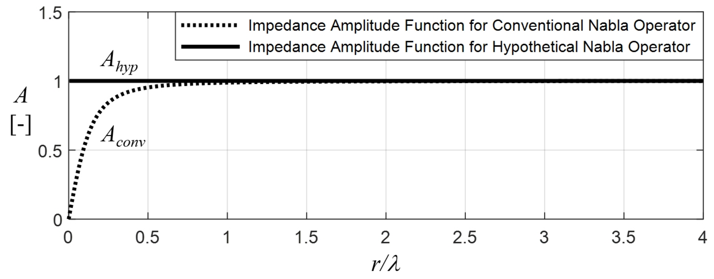
Following, the specific impedance $z=p/v$ is taken to show numerical differences between the two competing Nabla operator variants. According to Table 4 for the conventional (conv) Nabla operator the complex impedance $\underline{z}$ is normalized to $\rho c$ and transferred into polar form with the amplitude function A [-] and the phase $\varphi$ [rad]:

$$\frac{{\underline{z}}_{conv}}{\rho c}={\displaystyle \frac{{\left(kr\right)}^2+ikr}{1+{\left(kr\right)}^2}}=A_{conv}expi{\varphi }_{conv}$$

(24)

$$A_{conv}={\displaystyle \frac{kr}{\sqrt{1+{\left(kr\right)}^2}}}$$

(25)

$${\varphi }_{conv}=arctan\left(\frac{1}{kr}\right)=arccot\left(kr\right)$$

(26)

For the hypothetical (hyp) Nabla operator the impedance amplitude function $A_{hyp}$ [-] and the phase ${\varphi }_{hyp}$ [rad] have the following values

$$A_{hyp}=1$$

(27)

$${\varphi }_{hyp}=0$$

(28)

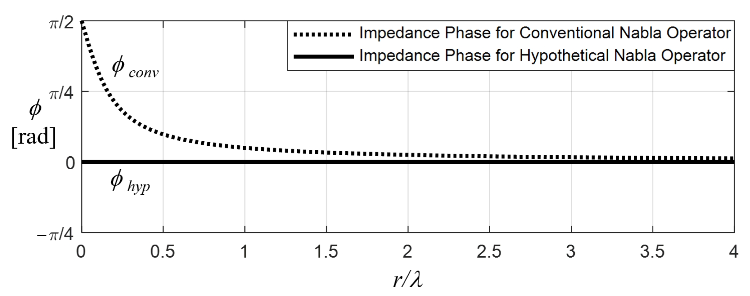
To illustrate the numerical differences between the conventional Nabla operator and the hypothetical Nabla operator variant Figure 1 shows the impedance amplitude functions and Figure 2 the phases depending on source distance r devided by wavelength $\lambda$ [m]; the value $r/\lambda$ [-] is taken because it is more easily comprehensible than $kr=2\pi r/\lambda$. According to both graphs, the conventional and hypothetical Nabla operator concepts substantially differ in the near field, but show asymptotic approximation in the far field. Because in many contexts of spherical wave propagation near field influences are neglected, above given spherical one-way wave equations and the hypothetical Nabla operator lead to significant simplifications of the related calculations.

5. Conclusions

With the spherical one-way wave equation and the hypothetical Nabla operator being presented in this paper the calculation of spherical wave propagation does not show wattless near fields and the solutions can be derived without the need of Bessel functions. Thereby spherical wave calculations can be significantly simplified.

References

- Seriani, G.; Oliveira, S.P. Numerical modeling of mechanical wave propagation. Riv. Del Nuovo C. 2020, 43, 459–514. [Google Scholar] [CrossRef]
- Angus, D.A. The One-Way Wave Equation: A Full-Waveform Tool for Modeling Seismic Body Wave Phenomena. Surv. Geophys. 2014, 35, 359–393. [Google Scholar] [CrossRef]
- Luo, M.; Jin, S. Halliburton Energy Services: Hybrid One-Way and Full-Way Wave Equation Migration. U.S. Patent US8116168, 14 February 2012. [Google Scholar]
- Bschorr, O. Deviationswellen im Festkörper [Deviation waves in solids]. In Proceedings of the DAGA 2014—40th German Annual Conference of Acoustics, Oldenburg, Germany, 10–13 March 2014; pp. 80–81. [Google Scholar]
- Bschorr, O.; Raida, H.-J. One-Way Wave Equation Derived from Impedance Theorem. Acoustics 2020, 2, 164–170. [Google Scholar] [CrossRef]
- Bronstein, I.N.; Mühlig, H.; Musiol, G.; Semendjajew, K.A. Taschenbuch der Mathematik [Handbook of Mathematics]; 10. überarbeitete Auflage; Europa Lehrmittel: Haan-Gruiten, Germany, 2018; pp. 731–733. [Google Scholar]
- Lerch, R.; Sessler, G.; Wolf, D. Technische Akustik [Technical Acoustics]; Springer: Berlin/Heidelberg, Germany, 2009; p. 33. [Google Scholar]
Figure 1.
Comparison of the impedance amplitude functions and for spherical wave propagation as a function of the normalized distance [-]. At the difference is 1.2%, for it is less than 0.14%. In practice, the near field influence is neglected in calculations.
Figure 2.
Comparison of the impedance related phases and as a function of [-]. For the angular difference is 0.158 rad resp. 9° and for less than 0.053 rad resp. 3°.