1. Introduction
A ‘Helmholtz resonator’ is a device in which a volume of compressible fluid is enclosed by rigid boundaries with a single, small orifice [
1]. The resonator is easily modelled by a second-order mass-spring system analogy, where the fluid in the region of the orifice acts as the effective mass, and the compressibility of the fluid in the volume acts as the stiffness. Acoustic radiation and viscous effects both lead to effective damping. The resonator’s natural frequency can be simply estimated as
, where
S is the area of the orifice;
l is the effective neck thickness;
V is the volume of the resonator; and
c is the speed of sound. Near this frequency, a small pressure disturbance can produce a large-magnitude velocity fluctuation at the orifice and thus a large pressure fluctuation within the resonator.
Such a resonance system can be excited acoustically at frequencies close to the resonance one. This feature is used for noise reduction applications. In this case, systems of one or several relatively large resonators (dimensions comparable to the typical scales of the flow) are used, for example, as installed on benchmarks [
2], when actually operating technical devices such as engines and fans [
3], and in covering materials with special perforations, in which some cells are like microresonators [
4]. Also, special metamaterials are being developed that use combinations of cavities (resonators) with different parameters for damping/selecting noise (see, for example, [
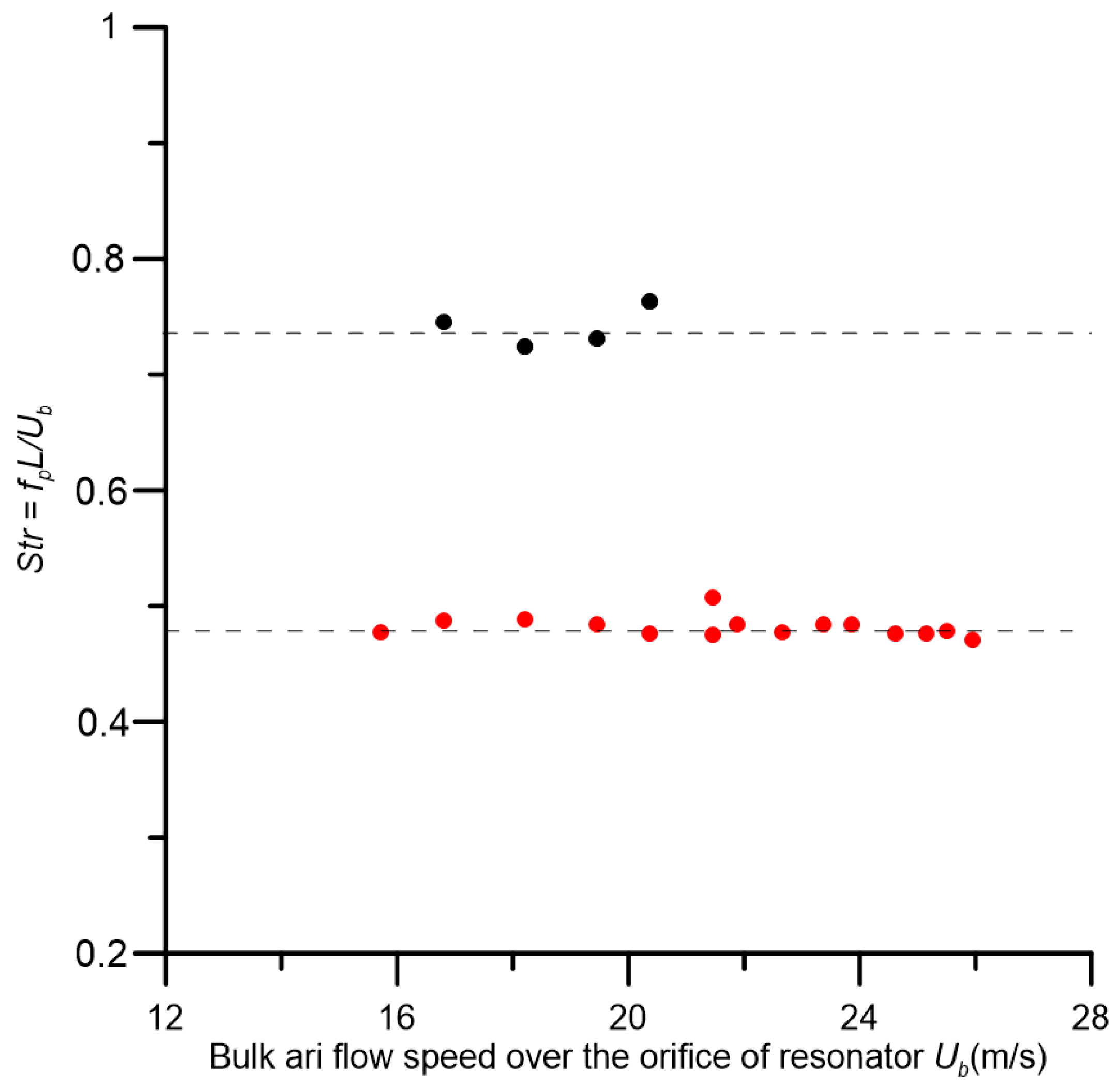
5]). But more interesting from a physical point of view is the so-called flow-excited resonator Helmholtz case. A very well-known example of this phenomenon is the resonance that occurs when blowing over the orifice of a glass bottle. The same physical process is present when an automobile is traveling with a single window lowered. This is often termed ‘window buffeting’ and results in an uncomfortable level of cabin pressure fluctuation. The physics of this process are that the shear layer is linearly unstable to disturbances for discrete numbers of the nondimensional Strouhal number
fL/
U (the parameter related to the generation of sound by unsteady flows), where
f is the oscillation frequency and
L is the size of the orifice along the flow (for example, [
6,
7]). In this case, the excitation of resonance oscillations generated by the flow occurs when one of the frequencies of hydrodynamic instability is close to the natural frequency of the resonator
fres. In other words, the pressure fluctuations in the resonator are the maximum at the specific velocity at which the frequency of the most unstable shear layer mode is equal to the frequency of the resonator. In most applications, notably for the glass bottle and automobile window, the velocity at which the fluctuations are the maximum will be at a relatively low Mach number, say
M < 0.1; however, compressibility cannot be neglected in these cases.
Early works on the study of the flow of the Helmholtz resonator mainly concerned the description of the acoustics of resonators of different sizes and configurations with different conditions of the exciting flow [
8,
9] without a detailed study of the mechanisms of occurrence of self-sustained oscillations. In [
10], detailed measurements of both the pressure in the resonator and the flow field near the orifice were carried out for the first time. These data were subsequently used to verify calculations in a number of studies. Thus, on their basis, in [
11], a flow analysis was performed based on the use momentum and energy budget in a linear approximation. The effect of orifice shape on fluctuations inside the resonator was studied in investigations [
12,
13,
14,
15]. For an orifice with a deep neck, a model based on the so-called feedback loops was proposed in [
16]. The hydrodynamic forcing was considered a “forward gain function” and the acoustics in the resonator were considered a “backward gain function”. The pressure amplitude inside the resonator was calculated by equating the amplitude and phase of the two gain functions. This method was further developed in [
17], in which an analytical description of the direct gain function was proposed. Using a certain dimensionless adjusting parameter
β, the theory was for the first time able to describe accurately the dependence of the pressure amplitude in the resonator on the free-stream velocity. Later, a modified version of this method by modeling the direct gain function in the point vortex approximation was developed in [
18]. This work demonstrates that it was possible to introduce an adjusting parameter
α that allowed the theory to accurately predict pressure in a resonator over a wide range of free-stream conditions.
The role of panoramic methods based on visualization in studying the characteristics of acoustic and hydrodynamic fields in the Helmholtz resonator problem should be mentioned, additionally. Thus, in [
19], studies of the parameters of resonance modes inside a resonator excited in an impedance pipe using fog visualization in a laser sheet was combined with the measurements of pneuma gauges and microphones. The fog visualization allowed a clear demonstration for the first time that resonance is caused by the disruption of a single discrete vortex from the edge of the orifice, which moves along it during one cycle of oscillations (the first mode) in studies of the flow-excited Helmholtz resonator ([
10]). A significant breakthrough was made in [
20], using well-established methods for measuring flow velocity fields’ Particle Image Velocimetry (PIV) (for a description, see [
21]). Here, the authors also used an analysis based on the use of the momentum equation to understand the relationship between the shear hydrodynamic instability of the boundary layer and the pressure instability in the resonator. They found that unsteady circulation (i.e., the integral area of the vortex over the orifice region) acted as a quantitative characteristic of the forcing on the resonator. The calculations of the pressure in the resonator carried out in [
20], based on the results of measurements of velocity fields, found good agreement within 3 dB with the results of measurements by microphones in a wide range of flow velocities. Thus, data on the flow velocity field near the orifice make it possible not only to obtain an estimation of the spatiotemporal structure of the hydrodynamic instability mode that initiates self-sustained oscillations, but also to obtain a quantitative estimate for pressure pulsations. Note that, unlike point measurements of sound pressure, PIV measurements of the velocity fields are very complex, especially on real technical systems. In this case, data on the flow velocity field can be obtained using computational fluid dynamics (CFD) numerical simulation, which is discussed below.
It should be noted that most of the laboratory measurements and theoretical studies use model conditions to evaluate the basic physical processes occurring in such systems. Thus, experiments with the free-flow-induced self-sustained oscillations are carried out in wind tunnels, where it is possible to control, vary and measure the flow parameters, or resonators are excited in special impedance pipes by controlled sound sources. In this case, resonators of the simplest configuration are used (rectangular, cylindrical, less often spherical, etc.), for which their own resonance modes can be measured/calculated well. Theoretical models developed using empirical data can describe such simplified problems well, but can often be used only for an approximate (qualitative) description of processes occurring in complex technical systems; for example, internal aeroacoustics of different vehicles (primarily car interiors), noise damping systems in various types of propulsion systems, climate control equipment, etc. Rapidly developing CFD methods can provide significant assistance here well as in many other studies of aero-hydrodynamic systems. However, the peculiarities of using CFD should be taken into account when the compressibility of the medium cannot be neglected, playing a fundamental role in the systems considered in this work.
Taking into account that compressibility leads to the need to solve an additional equation connecting pressure and density changes, this inevitably leads to an increase in resource costs compared to the incompressible formulation. In addition, it should be noted that acoustic disturbances in amplitude are of a much lower order than disturbances associated with the formation of vortex structures, which is why it is often necessary to use data storage in a 64-bit system, instead of in a 32-bit system, which is sufficient for incompressible productions. This affects the required RAM doubling, which for large problems (in terms of the number of grid model elements) is no less problematic than the calculation speed.
Another complicating factor is concerned with adjusting the discretization time step in calculations. A Courant–Friedrichs–Lewy criterion, which characterizes the disturbance spatial transfer in space over a fixed time interval, is used for choosing this important parameter in CFD procedures:
where
,
,
are components of velocity transfer,
,
,
are the spatial discretization scale, and
is the discretization time step. Criterion (1) means that the disturbance should not be advected more than the spatial discretization scale per time step. Here, again, we should recall the fundamental need to take into account compressibility for the occurrence of self-sustained oscillations in the systems under consideration in this work, despite the fact that the velocities of the exciting flow above the hole satisfy the condition
M ≪ 1. Taking into account condition (1), for such problems the time step must be reduced by
n =
c/
U times, with a corresponding increase in calculation time by
n times compared to problems of incompressible flows.
Seeking a compromise between the quality of the results obtained (usually verified with measurement data), greediness resources and calculation time is a usual feature when using CFD methods to study any hydrodynamic system, and especially when solving applied problems for various kinds of complex technical devices. The need to take into account the compressibility of the medium, which is the main factor in systems such as the Helmholtz resonator considered in this work, leads to higher resource/time requirements compared to an incompressible medium. In this regard, attempts to use simplified approaches to describe Helmholtz resonators excited by flows have been made from the very beginning of the use of CFD methods. For example, in [
19], a certain intermediate approximation was used between the conditions of a compressible and incompressible medium for the Navier–Stokes equations, and in [
20] a numerical procedure based on the kinetic equation, combined with the RNG turbulence model, is applied. In this case, it was possible to obtain good qualitative agreement; however, the calculated amplitudes of pressure pulsations could be lower (up to 20 dB, see [
19]), and in [
20] a special coefficient was even introduced to reduce the free flow velocity by 15/22 times compared to parameters of the experimental studies in [
10] to demonstrate agreement between the calculated pressure values in the resonator and the experimental data. This was explained by the difficulties of adequately reproducing the velocity distribution in the boundary layer, the thickness of which affects the effective velocity of the shear layer. On the other hand, when carrying out calculations without any simplifications for modeling specific structures, resource greediness increases greatly. For example, in work [
22], to calculate the buffering effects from a window inside a simplified model of a car like the Purdue cavity model with a scale of about 1:5 of the real size, it took 7 days of calculations for an implementation lasting only 0.25 s on a grid of 16 million nodes to achieve an accurate determination of pressure pulsations on the main modes of at least 10 dB (in comparison with a verification experiment in a wind tunnel).
It should be mentioned that no special research devoted to the choice of correct and optimal calculation parameters to obtain results with the required accuracy when solving problems of Helmholtz resonator excitation by a free flow has been carried out to solve this urgent problem. This work is intended to at least partially fill this gap.
The article has the following structure. The first part describes a special laboratory experiment performed in the wind tunnel of the Institute of Applied Physics RAS, the results of which were used to verify numerical model. The second part is devoted to a description of calculation procedures, including the turbulence models used, the computational grids, and a comparison of the results obtained with the experiments performed. At the end, there are the main conclusions.
3. Numerical Modeling
3.1. Calculation of the Frequency Response of the Resonator
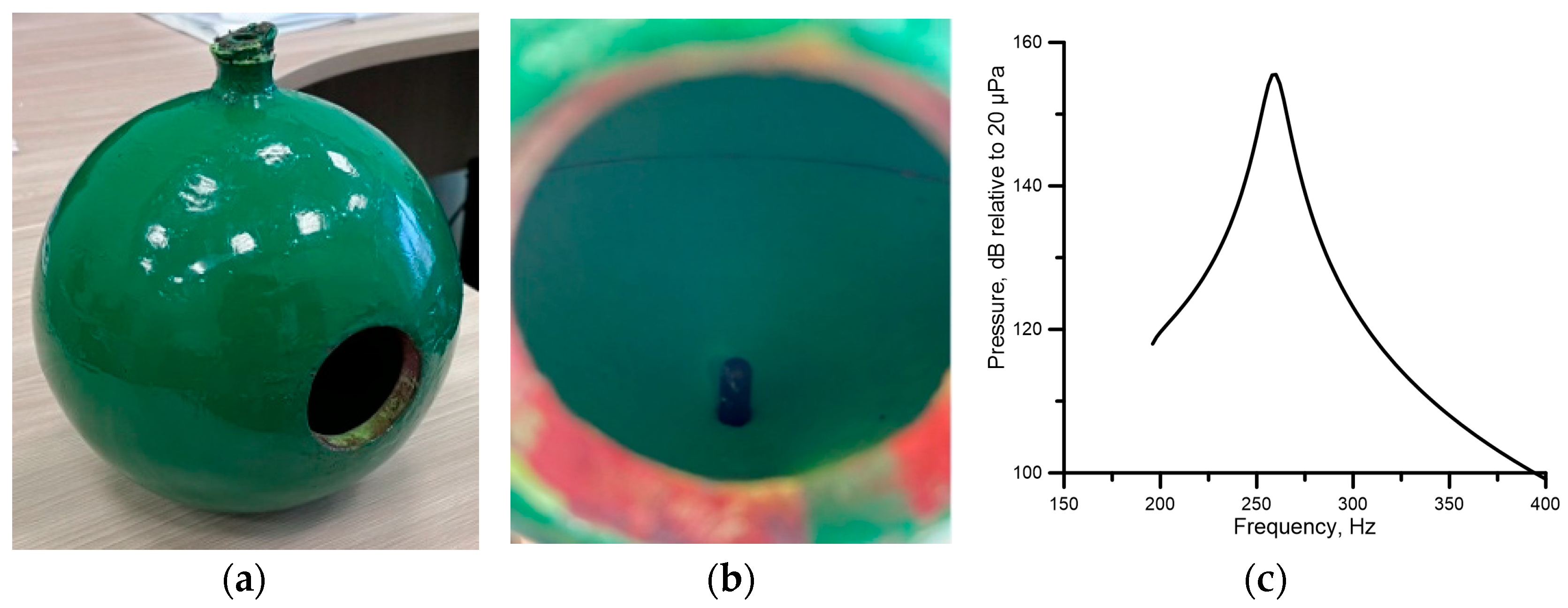
The resonance frequency response characteristic of the spherical resonator in our work was obtained numerically by using the finite-element model within original software “SATES”. The acoustic finite element model represented a spherical resonator surrounded by air volume. The walls of the resonator were modeled as a rigid body, on the outer boundary of the spherical air volume impedance elements installed, which made it possible that no reflection of the acoustic waves came back into the computational region. The excitation of the resonator was simulated by a single dipole source located at the center of the orifice and oriented along the
x axis.
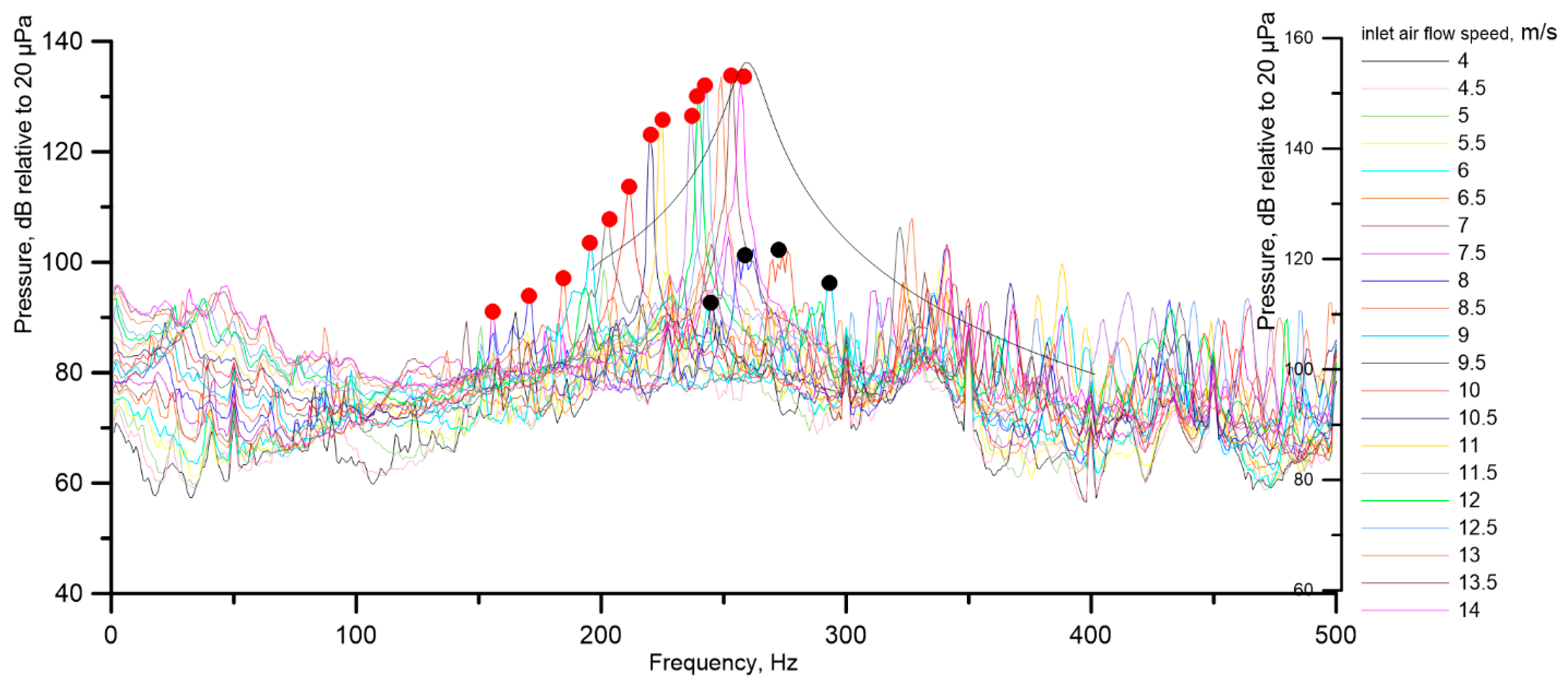
Figure 8 shows the numerical model used by the software SATES 2.0. Red lines show impedance elements. The calculation result (earlier, in
Figure 1) and the frequency response are shown together with the measurement results in
Figure 5.
3.2. Description of Procedures of Numerical Modeling of Aeroacoustics, Calculation Results, and Comparison with Experimental Data
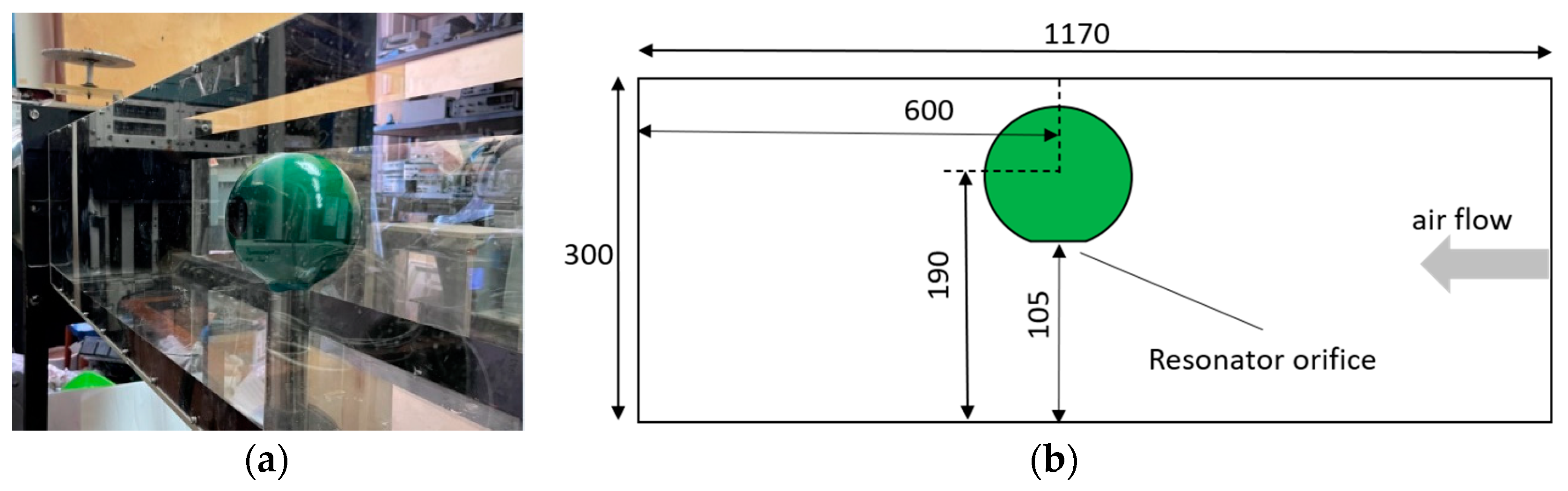
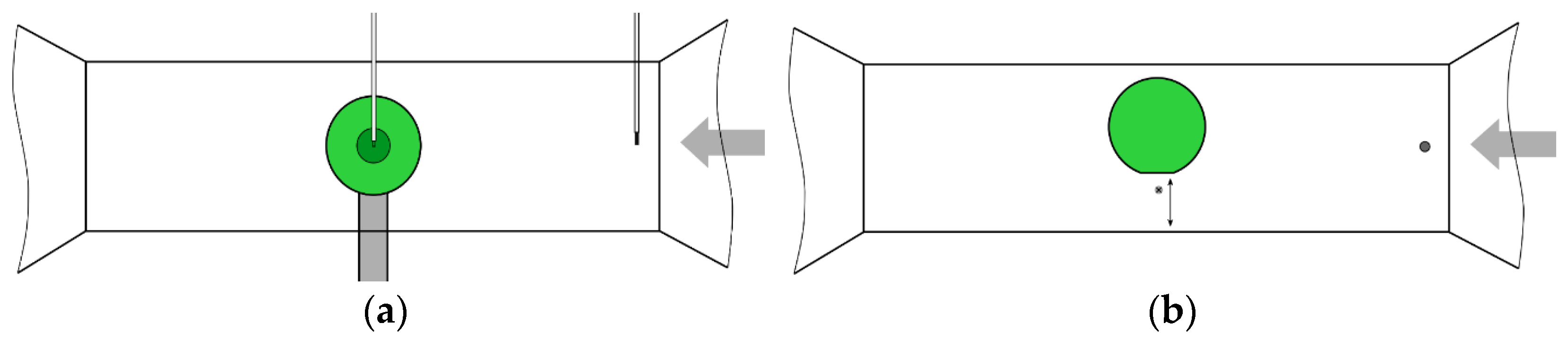
Calculations were performed for the air flow around a spherical resonator within the configuration, similar to the verification experiment on the wind tunnel described in the previous section.
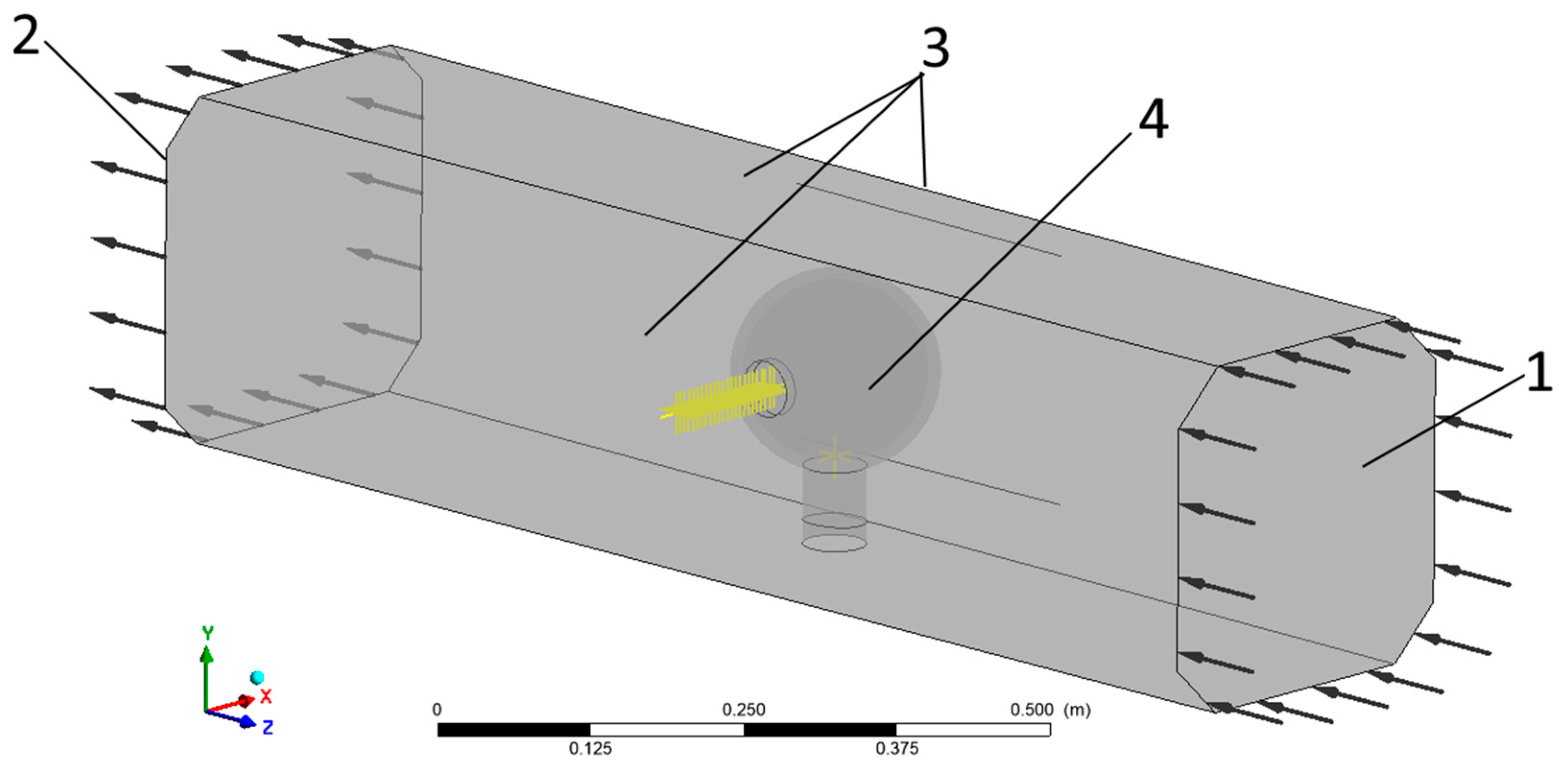
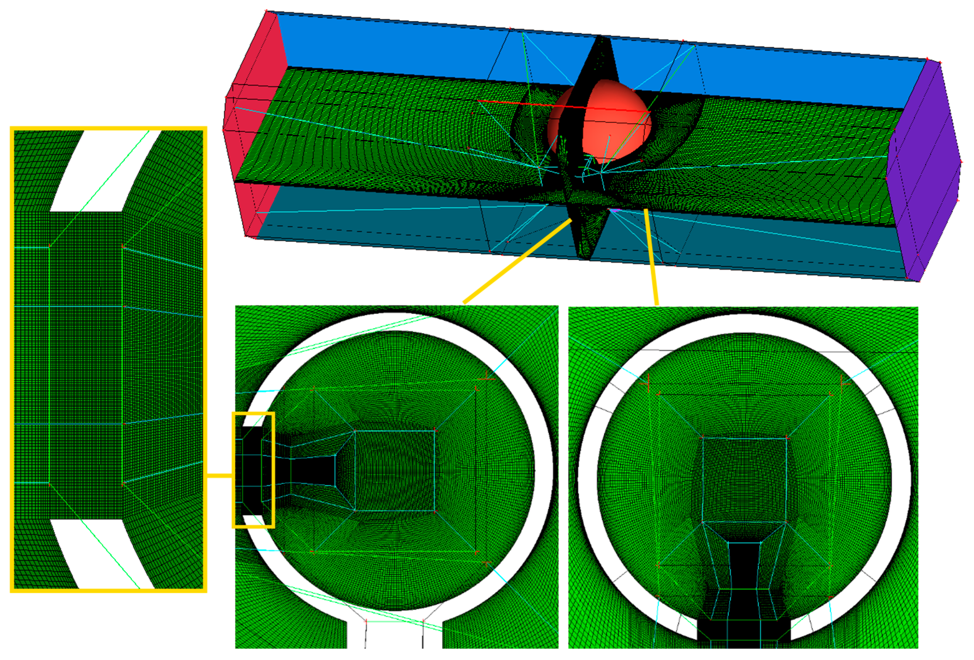
Figure 9 shows the computational domain, including the Helmholtz resonator (with geometric characteristics that fully corresponded to the laboratory experiment), placed in the working section of the wind tunnel, by analogy with the laboratory experiment. Yellow markers are control points, in which values of the three velocity components and pressure were recorded during the solution process for further processing.
The inlet airflow speed was set at the input boundary of computational domain (see the
Figure 9) 1 with a turbulence intensity of 1%. This speed was equal to that in the experiment. The average pressure excess at outlet boundary 2 was assumed to be zero, and the condition of no slip was specified on the side walls of the working section 3 and the surface of the sphere 4.
The solution of the problem In the first formulation was carried out using the simplest turbulence model from the URANS class. In the context of this turbulence model, the averaged Navier–Stokes equations for a compressible ideal gas are solved and described by the following equations (while the time averaging signs are omitted for brevity):
Here, are the Cartesian coordinates (k = 1, 2, 3); are the components of the velocity vector of the averaged flow; E and H are the specific total energy and total enthalpy of the gas; T is the temperature; R is the universal gas constant; and m is the molecular mass. The components of the molecular viscous stress tensor and the heat flux density vector due to the molecular thermal conductivity are determined, respectively, using Newton’s rheological law and Fourier’s law. The components of the Reynolds stress tensor and the Reynolds heat flux vector are determined using Mentor’s Shear Stress Transport (SST) turbulence model.
The two-parameter turbulence model SST has the following formulation:
where
F1 function is a switch between
k-ω and
k-ε turbulence models.
This model of turbulence was used due to the assumption that it is necessary to determine the narrowband component of the frequency spectrum of velocity pulsations. This peak corresponds to the frequency of vortex shedding from the leading edge of the orifice, which is synchronized with the resonance frequency of the resonator volume.
This approach demands relatively small requirements (in comparison with the scale resolving simulation approach) for the computational grid model, i.e., to resource greediness. The Menter’s SST turbulence model (SST) was used to close the system of Reynolds-averaged Navier–Stokes equations.
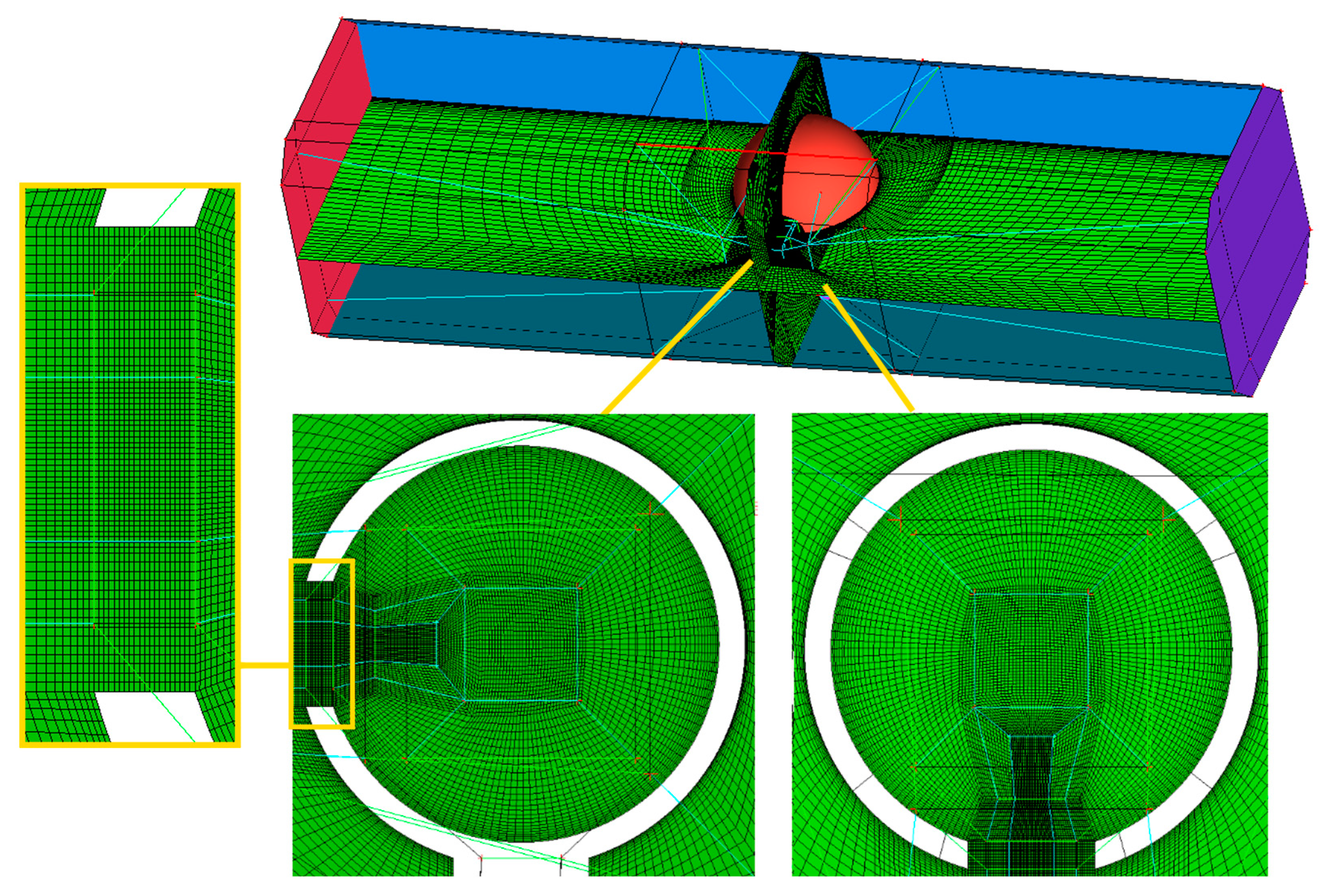
A block-structured grid model in the computational domain divided into cells consisting of hexahedral elements was used.
Figure 10 shows a general view of the grid model GM1 (1.2 million cells) with selected fragments near the resonator, developed to formulate the problem using the SST turbulence model.
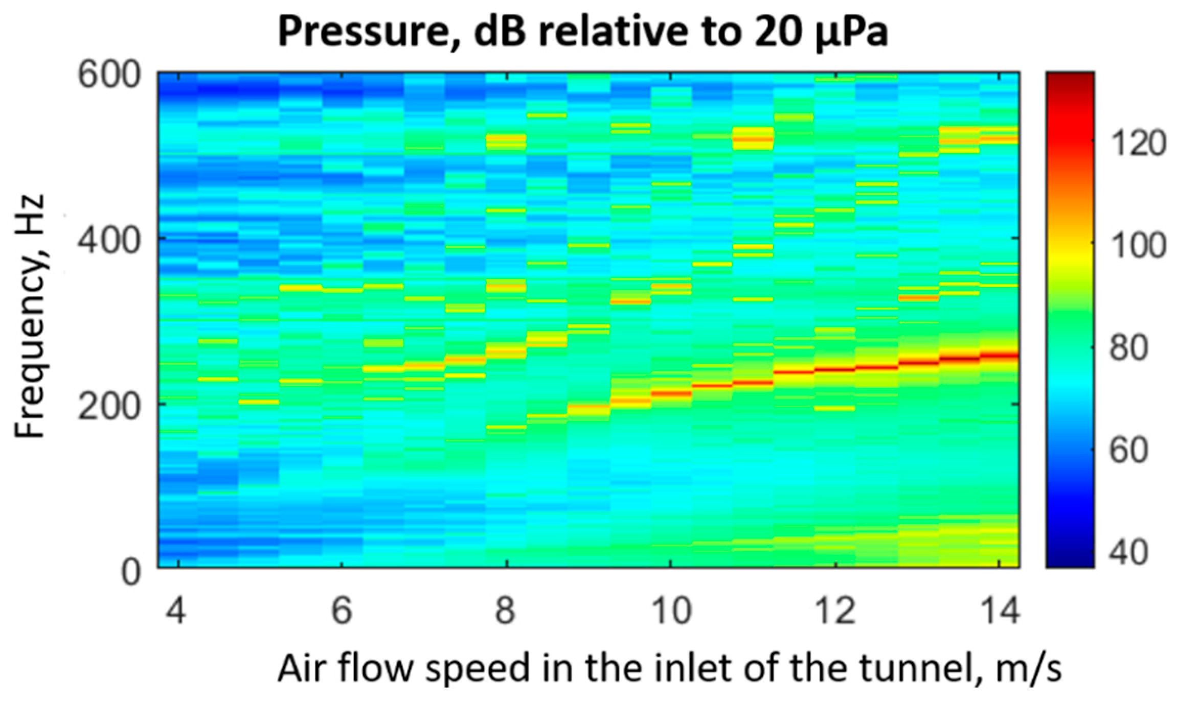
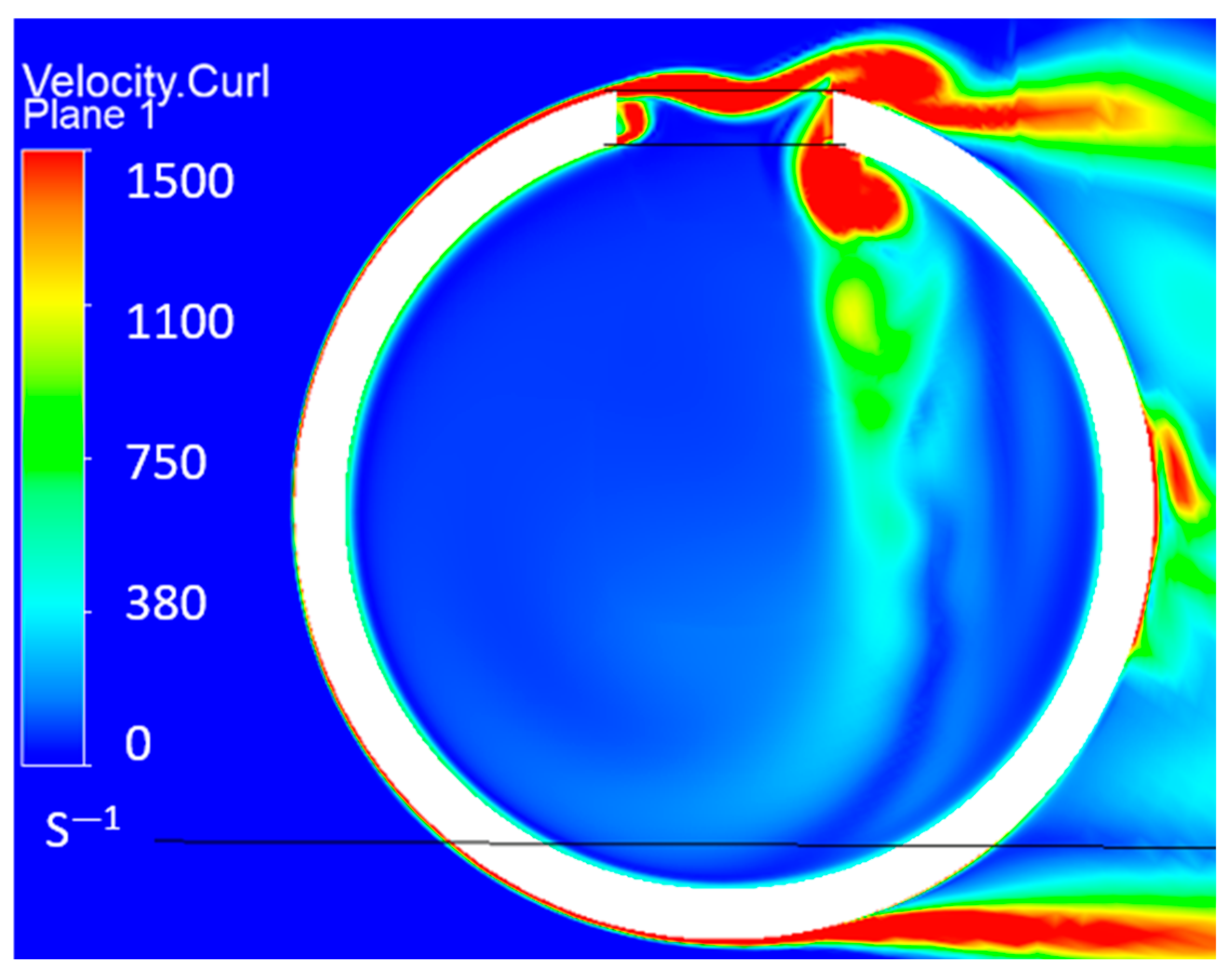
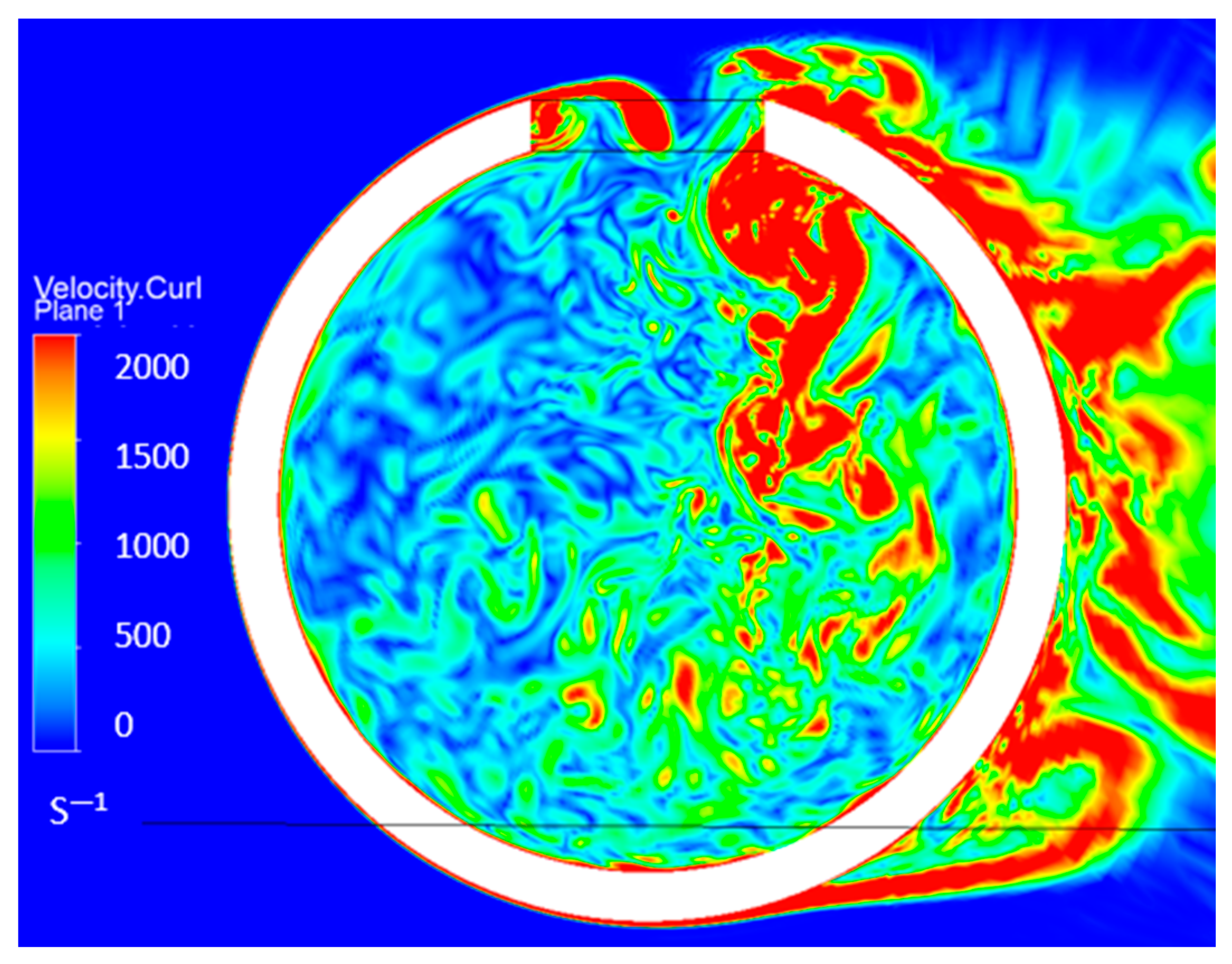
Fields of hydrodynamic characteristics (velocity, vorticity, pressure) were obtained inside the computational domain determined on the grid model GM1. The vorticity field at the cross-section plane of symmetry of the resonator at the inlet airflow speed of 14 m/s is shown in
Figure 11. It was possible to simulate the process of shedding of a vortex from the leading edge of the orifice and its transfer to the trailing edge by analogy with the works [
10,
20].
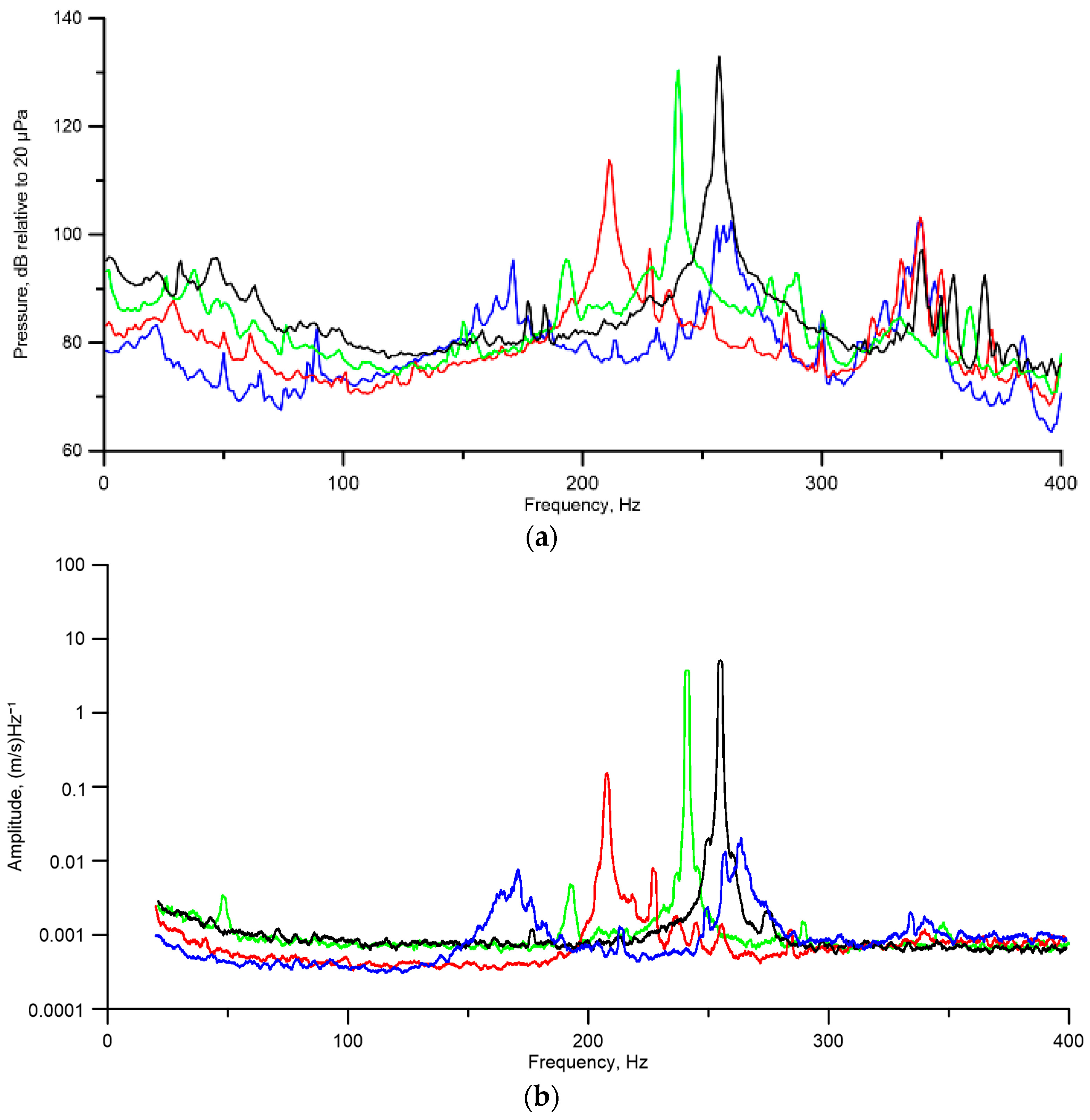
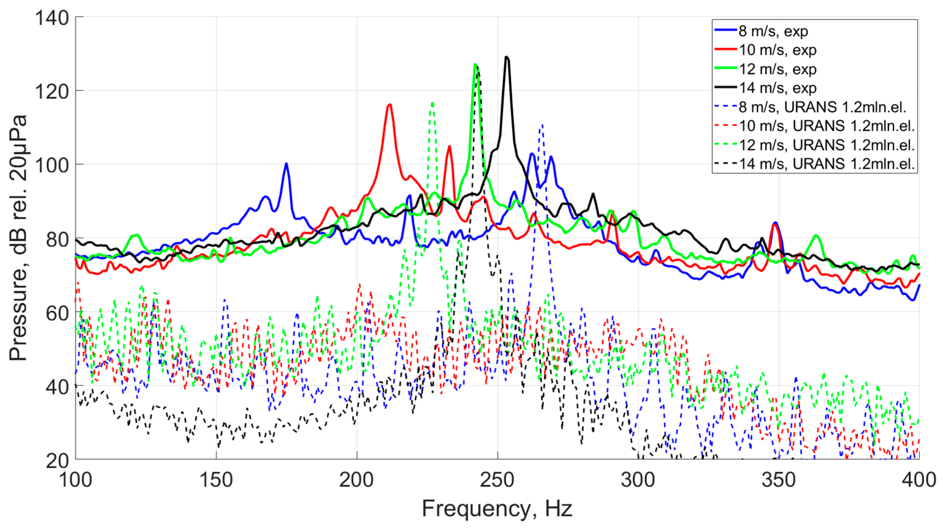
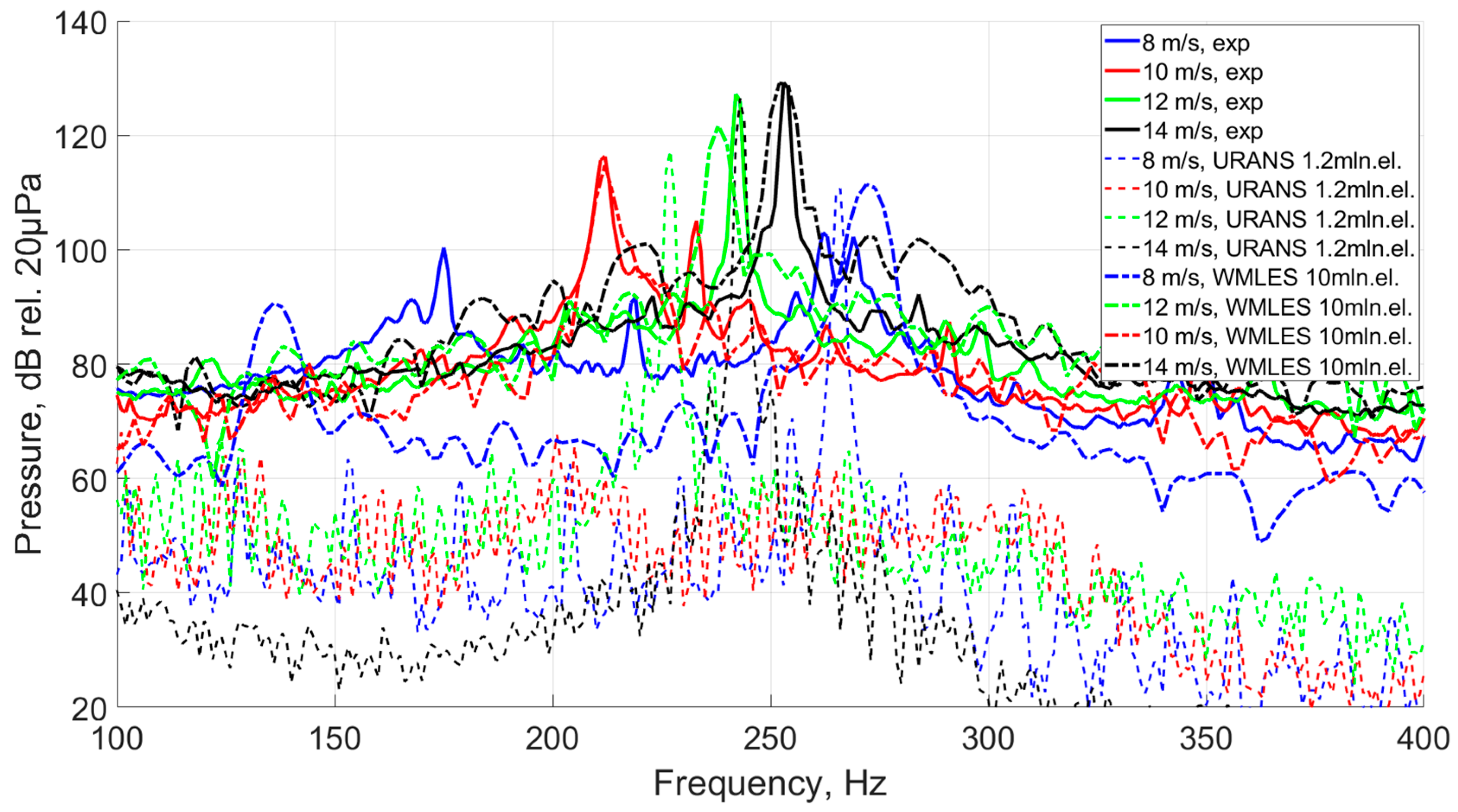
A comparison of the calculated pressure pulsation power spectra in the center of the resonator for four different flow rates (8, 10, 12, 14 m/s) for the SST model (dashed lines) with those measured experimentally in the wind tunnel (solid lines) is shown in
Figure 12.
Narrowband peaks in the spectrum corresponding to the frequencies of vortex shedding from the leading edge were well distinguished. At speeds of 12 and 14 m/s, the discrepancy between the calculation and experiment frequency for peaks was about 4–6%, and in pressure level 3–10 dB. The data are inconsistent at the 10 m/s transient regime due to the specific property of the SST turbulence model. The feature is concerned with setting the averaging period of hydrodynamic fields relative to energy-transfer vortices using the model. Here, this period is determined by the frequency of the dominated non-stationary process in the system, and since the mode of instability changes from the first to the second with approximately the same order of magnitude, there is an uncertainty in the choice of the averaging period (frequency of dominating energy-transfer vortices) at a speed of 8–10 m/s. It should be noted that the SST turbulence model does not reproduce background turbulence, and therefore the characteristics studied outside the resonant frequency cannot fundamentally coincide with experiment.
To compare with the results of SST modeling, another numerical model was used for calculations in the scale-resolving simulation (SRS) using the WMLES (Wall-Modeled Large Eddy Simulation) model based on the same SST model. The mathematical formulation of this approach differs from RANS only in the description of additional terms in the right part of the equations of motion and energy. Instead of the components of the Reynolds stress tensor and the Reynolds heat flux vector (see the Formula (2), there are spatially filtered (but unlike the RANS formulation, there are instantaneous values of the terms here) nonlinear convective terms of the Navier–Stokes equations and , where the sgs indices indicate a sub-grid scale.
In the context of this turbulence model, all the disturbances with scales that were larger than several cells of the grid model were directly resolved, and the energy of unresolved turbulence of smaller scales was compensated by sub-grid viscosity. In this case, the boundary layer was divided into two parts because of the requirement for the fineness of the grid model due to the significant decrease in the scale of energy-transfer vortices as we became closer to the streamlined wall in the boundary layer. The SRS model operates in the outer region (as in the free flow), and near the wall the SST model is activated, which compensates for the unresolved part of the boundary layer energy.
To formulate the problem using the WMLES turbulence model, the sizes of the grid elements were reduced by half compared to SST. Thus, the grid model GM2 was formed (see
Figure 13). The total number of elements in GM2 was almost 10 million.
An example of the obtained vorticity field using the WMLES model at the cross-section plane of symmetry of the resonator at the inlet airflow speed of 14 m/s is showed on
Figure 14. Comparing
Figure 11 and
Figure 14, it is clear that the vortex structure formed at the leading edge of the resonator orifice, breaking up on the lower edge, fragments up into smaller vortex structures and their intensity is greater, compared to the results with the URANS formulation.
The pressure pulsation spectra obtained in the SRS formulation (dashed lines) are presented together with the previous results for the URANS formulation in
Figure 15 for similar flow conditions. There is a good agreement between the levels and frequencies of resonances for velocities of 10, 12 and 14 m/s with experimental data. Moreover, the calculations better reproduce the background level of pulsations, in contrast to the SST turbulence model. The spectral peaks of the resonances, due to the short total time realization, have a larger width than in the experiment, which can be eliminated by the accumulation of a longer time realization during the calculation process in further investigations. For the transition regime at an inlet speed of 8 m/s, where a rivalry between the first and second modes of hydrodynamic instability occurred, the discrepancy with the experiment is significant (25% in frequency and 10 dB in level) for the first mode. For the second mode at this speed, the frequency error is only 2% if we consider it relative to the middle of the wide peak obtained from the experimental results.
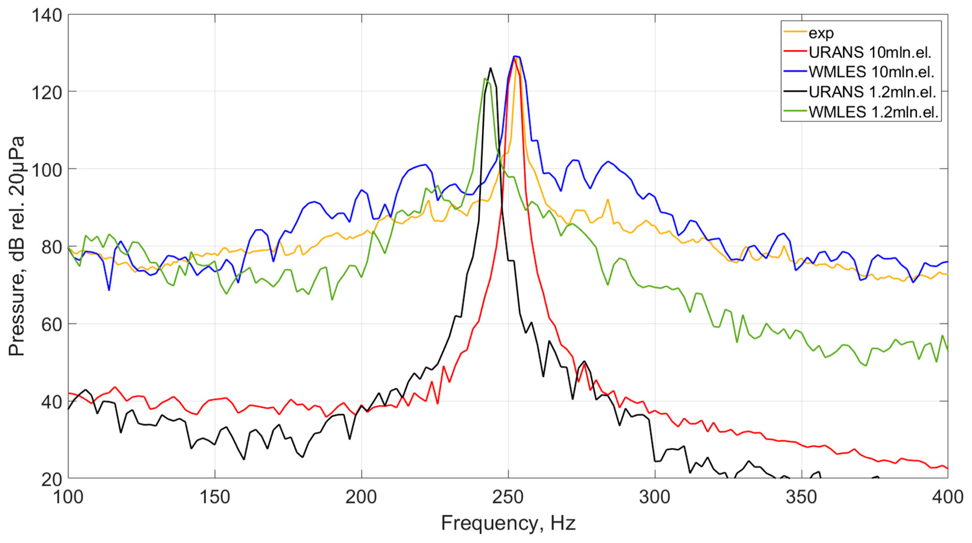
The influence of grid model parameters on the resulting hydrodynamic characteristics for the SST and WMLES turbulence models has different behavior. A refinement of the grid model in the case of the SST model (mainly in the unsteady flow region) leads to convergence on the “model” solution, determined by the settings of the turbulence model. In the WMLES model, the refinement of the grid model brings us closer to the direct solution of the Navier–Stokes equations, which describe the physical process “as it is”, in contrast to the previous one. To clarify the effect of refinement of the grid model on the hydrodynamic characteristics for this problem, the SST and WMLES turbulence models were used with both of the GM2 and GM1 grid models, respectively.
The SST turbulence model on the finer grid model GM2 allowed one to determine the pressure inside the resonator more accurately, as is shown in
Figure 16. This indicates the correct settings of the turbulence model for this class of problems (constants set by the default in software). Moreover, in terms of accuracy, they are completely close to the results obtained in the SRS formulation with the same grid model. The results of solving the problem using the WMLES turbulence model in combination with the less-fine grid model GM2 gave some unexpected results (from the first point of view). An increase in the size of the elements led to not only a decreasing amplitude of pulsations at the resonance frequency, which looked true because less energy can be resolved directly in this case, but also to a shifting of the resonance frequency. This effect may be associated with the evaluation of the boundary layer in the region above the orifice, where the flow becomes unstable. To confirm this assumption, additional research with a finer grid in the boundary layer in the area of the orifice with the same grid parameters outside the boundary layer is needed.
From the point of view of resource greediness, expressed in the number of core hours spent on obtaining a solution, both turbulence models turned out to be almost equivalent when using the same grid models. This is most likely due to the implementation of numerical schemes, as well as turbulence models in specific software.
Table 1 summarized the data on the resources spent in solving this problem, expressed in processor time—the number of cores involved in solving multiplied by the time (in hours) of the solver for all arrangements of numerical modeling. The characteristics of a high-performance computer system are two processors with 20 Intel(R) Xeon(R) Gold 6230 cores at a frequency of 2.10 GHz.
The advantage of the WMLES turbulence model compared to SST (from the point of view of the determined frequency response) is concerned with the correct estimation of background turbulence outside the narrowband resonance. This can be useful in studies where, in addition to the well-pronounced resonance frequency due to the effects of compressibility of the media inside the resonator, the system also contains structural resonances at which, under the influence of a broadband source, the level of acoustic radiation can also locally increase.


 ,
, 


