A Numerical Study on Computational Time Reversal for Structural Health Monitoring

Abstract

Structural health monitoring problems are studied numerically with the time reversal method (TR). The dynamic output of the structure is applied, time reversed, as an external loading and its propagation within the deformable medium is followed backwards in time. Unknown loading sources or damages can be discovered by means of this method, focused by the reversed signal. The method is theoretically justified by the time-reversibility of the wave equation. Damage identification problems relevant to structural health monitoring for truss and frame structures are studied here. Beam structures are used for the demonstration of the concept, by means of numerical experiments. The influence of the signal-to-noise ratio (SNR) on the results was investigated, since this quantity influences the applicability of the method in real-life cases. The method is promising, in view of the increasing availability of distributed intelligent sensors and actuators.

1. Introduction

The detection and localization of defects, based on measurements at a limited number of spatial points, falls into the category of inverse problems which are usually ill-posed and difficult to solve. Dynamical signals have the ability to detect hidden defects, and provided that measurements can be postprocessed effectively, are very useful for structural health monitoring purposes. The availability of cheap and interconnected sensors and data processing power facilitate practical applications.

Structural health monitoring (SHM) problems are based on the postprocessing of suitable measurements in order to monitor the structural health of a structure. Warning, in case of significant changes from the healthy nominal model, is the first stage of SHM. The qualification and quantification of damages and other deviation from the nominal structural model are subsequent, more delicate tasks. They belong to the class of inverse and parameter identification problems, which lead to ill-posed mathematical problems that require delicate numerical processing tools. A general solution of inverse and parameter identification problems in mechanics can be based on the comparison of predictions based on suitably parametrized models with measurements, using optimization or soft computing, as can be seen in [1,2,3,4], among others. A computational tool for solving a class of inverse wave (and/or vibration) problems is the time reversal (TR) technique originally introduced as a physical process [5]. Time reversal concepts have been raised in several scientific communities and seems to be an object of high interest for mathematicians, physicists and engineers. Time reversal is a technique that focuses waves onto a source or scatter by emitting a time-reversed analogue of the received wave field measured by an array of transducers. This refocusing is due to the reciprocity in space and reversibility in time for the wave field [6,7]. The main idea behind TR is to send the recorded signals back into the medium but reversed in time. Due to the time-reversibility of the wave equation, this process created a back propagating wave that will focus on the original source location. A defect or damaged area can be understood to act as a secondary source and therefore the principle of TR can be used to find its location.

The TR method has been used for the impact location determination in [8,9] and for both impact location and force identification in [10,11]. Lamb waves in connection with TR have been used in several works for the detection of micro-cracks in plates and composite structures [12,13,14,15,16,17,18,19,20]. Good experimental results have been reported in several publications like [11,21]. Further information can be found in the review publications [22,23,24]. The technique has possible applications in difficult nonlinear identification problems, like the breathing unilateral crack identification [25]. Furthermore, it can be used within active SHM systems, incorporating modern deep learning techniques in order to solve difficult identification problems [26].

Frame structures that are excited by some loading on respective source points called $x_s$ are considered in this paper. The response is collected on a number of points called receivers $x_r$. Each receiver is defined by a pair of its spatial location and the direction on which response is recorded and then we use time-reversal as an imaging technique in order to detect and localize the defect. Receivers collect data for selected degrees of freedom (DOFs) on some nodes, that for the used beam elements, are the axial, transverse and rotational motions. For the source localization procedure, it is necessary to reverse the responses of every receiver in time and from now on the receivers operate as actuators because they transmit the reversal responses for each receiver/stimulator and save the results on the selected point to use for imaging. These points will be referred to as the imagers $x_i$. Furthermore, we assume that we can measure or reproduce the scattered field produced by some scatterer, that is the difference between the total field recorded in the presence of the defect and the incident field which corresponds to the healthy structure. Our approach is purely computational and therefore the response recordings are being produced numerically (the so-called, pseudo-experiment). Because of reflections from the boundaries, the scattered field is complicated and might appear at multiple arrival time peaks.

Following work in the field of acoustics [27], the objective of this paper is to show that the time-reversal invariance can be exploited in the context of structural dynamics to accurately control wave propagation and to improve target detection through structures. In this work, we introduce the computational time reversal approaches for engineering structural problems focusing, but not confined, to frame structures. The investigation is purely numerical, utilizing the so-called pseudo-experiments. Nevertheless, in view of future experimental verification, the important influence of the signal-to-noise ratio was investigated for various numbers and placements of sensors.

The paper is structured as follows. The theory of time reversal refocusing from a reciprocity theorem’s perspective is presented in the next section. Section 3 presents the computational dynamics steps used for the implementation of the method, including the consideration of stochastic Gaussian noise and signal-to-error sensitivity analysis. The numerical results are presented in section four. The next session presents some investigations relevant to optimal sensor placement. The paper closes with conclusions and proposals for further research.

2. Time Reversal Approaches for Structures

Our vehicle to present and justify time reversal approaches for structures would be the elastodynamics reciprocal theorems, with a focus on frame structures. For convenience, we will set up dynamics reciprocity for the Euler–Bernoulli beam theory as well as for the axial wave propagation in a rod. Such reciprocity could be considered as an extension of the classical Betti’s theorem [28] when inertial forces are also considered. It has been shown in [29] that Betti’s theorem could be seen as a degeneration of the elastodynamics reciprocal theorem in terms of velocities.

2.1. Elastodynamic Reciprocity for Classical Beam Theory

The basic assumption of the Euler–Bernoulli theory is that a plane cross-section, perpendicular to the axis of the beam, remains plane and perpendicular to the neutral axis during bending. The differential equation of motion for a beam, considering both materials’ density and cross-section constant over the beam’s axis x is given as

$$\begin{array}{c}\hfill EI\frac{{\partial }^{4}u}{\partial x^4}+\rho A\frac{{\partial }^{2}u}{\partial t^2}=q(x,t)\end{array}$$

(1)

with the boundary conditions distinguished as the essential ones defined on $x\in {\Gamma }_u$:

$$\begin{array}{cc}\hfill & u(x,t)=\overline{u}(x,t),\hfill \end{array}$$

(2a)

$$\begin{array}{cc}\hfill & \frac{\partial u(x,t)}{\partial x}=\overline{\psi }(x,t)\hfill \end{array}$$

(2b)

and the natural ones defined on $x\in {\Gamma }_t$:

$$\begin{array}{cc}\hfill & -EI\frac{{\partial }^{2}u(x,t)}{\partial x^2}=\overline{M}(x,t),\hfill \end{array}$$

(2c)

$$\begin{array}{cc}\hfill & -EI\frac{{\partial }^{3}u(x,t)}{\partial x^3}=\overline{Q}(x,t).\hfill \end{array}$$

(2d)

with $\overline{M}$ and $\overline{Q}$ indicating the prescribed bending moment and shear force, respectively. The necessary initial condition to accompany the above system are:

$$\begin{array}{cc}\hfill & u(x,0)=u_0\left(x\right),\hfill \end{array}$$

(3)

$$\begin{array}{cc}\hfill & \frac{\partial u(x,0)}{\partial t}={\dot{u}}_0\left(x\right).\hfill \end{array}$$

(4)

We now consider a continuous function $v(x,t)$ which is assumed to be the displacement field for some other elastodynamic configuration for the same beam under loading distribution $w(x,t)$.

We recall at this point the definition of Riemann convolution. Riemann convolution of functions $f\left(t\right)$ and $g\left(t\right)$ is defined as

$$g\left(t\right)\ast h\left(t\right)=\left\{\begin{array}{cc}\underset{0}{\overset{t}{\int }}g(t-\tau )h\left(\tau \right)d\tau ,\hfill & \mathrm{for}t>0\hfill \\ 0,\hfill & \mathrm{elsewhere}.\hfill \end{array}\right.$$

(5)

Taking the Riemann convolution in time of function $v(x,t)$ with equation of motion (1) and integrating over the x-axis we obtain:

$$EI\underset{0}{\overset{L}{\int }}\frac{{\partial }^{4}u}{\partial x^4}\ast vdx+\underset{0}{\overset{L}{\int }}\rho A\frac{{\partial }^{2}u}{\partial t^2}\ast vdx=\underset{0}{\overset{L}{\int }}q(x,t)\ast vdx.$$

(6)

The first integral of (6) after sequential integration by parts can be written as

$$\begin{array}{c}\hfill EI\underset{0}{\overset{L}{\int }}\frac{{\partial }^{4}u}{\partial x^4}\ast vdx=EI\underset{0}{\overset{L}{\int }}u\ast \frac{{\partial }^{4}v}{\partial x^4}dx+EI{\left[\frac{{\partial }^{3}u}{\partial x^3}\ast v-\frac{{\partial }^{2}u}{\partial x^2}\ast \frac{\partial v}{\partial x}+\frac{\partial u}{\partial x}\ast \frac{{\partial }^{2}v}{\partial x^2}-u\ast \frac{{\partial }^{3}v}{\partial x^3}\right]}_0^L.\end{array}$$

(7)

The integral of (6) concerning inertial terms taking advantage of time convolution’s identities can be written as

$$\begin{array}{c}\hfill \rho A\underset{0}{\overset{L}{\int }}\frac{{\partial }^{2}u}{\partial t^2}\ast vdx=\rho A\underset{0}{\overset{L}{\int }}u\ast \frac{{\partial }^{2}v}{\partial t^2}dx+\rho A\underset{0}{\overset{L}{\int }}{\dot{v}}_{0}u+v_0\dot{u}-{\dot{u}}_{0}v-u_0\dot{v}dx.\end{array}$$

(8)

Substitution of (7) and (8) into (6), taking under consideration that $v(x,t)$ is the displacement field for the distributed loading $w(x,t)$ results in the reciprocal relation between states of ($u,q$) and ($v,w$), that is:

$$\begin{array}{cc}\hfill & \underset{0}{\overset{L}{\int }}w(x,t)\ast u(x,t)dx-\underset{0}{\overset{L}{\int }}q(x,t)\ast v(x,t)dx=\hfill \\ \hfill & EI{\left[\frac{{\partial }^{3}u(x,t)}{\partial x^3}\ast v(x,t)-\frac{{\partial }^{2}u(x,t)}{\partial x^2}\ast \frac{\partial v(x,t)}{\partial x}+\frac{\partial u(x,t)}{\partial x}\ast \frac{{\partial }^{2}v(x,t)}{\partial x^2}-u(x,t)\ast \frac{{\partial }^{3}v(x,t)}{\partial x^3}\right]}_0^L\hfill \\ \hfill & +\rho A\underset{0}{\overset{L}{\int }}{\dot{v}}_0\left(x\right)u(x,t)+v_0\left(x\right)\dot{u}(x,t)-{\dot{u}}_0\left(x\right)v(x,t)-u_0\left(x\right)\dot{v}(x,t)dx.\hfill \end{array}$$

(9)

As shown in what follows, the above reciprocal relation could serve as the starting point of time reversal approaches for the case of the Euler–Bernoulli beam. Furthermore, such an approach could be easily adapted in other cases of structural dynamics, e.g., axial waves, Timoshenko beam theory, or to the more general linear elastodynamic case.

2.2. Time Reversal Refocusing as Outcome of Reciprocity

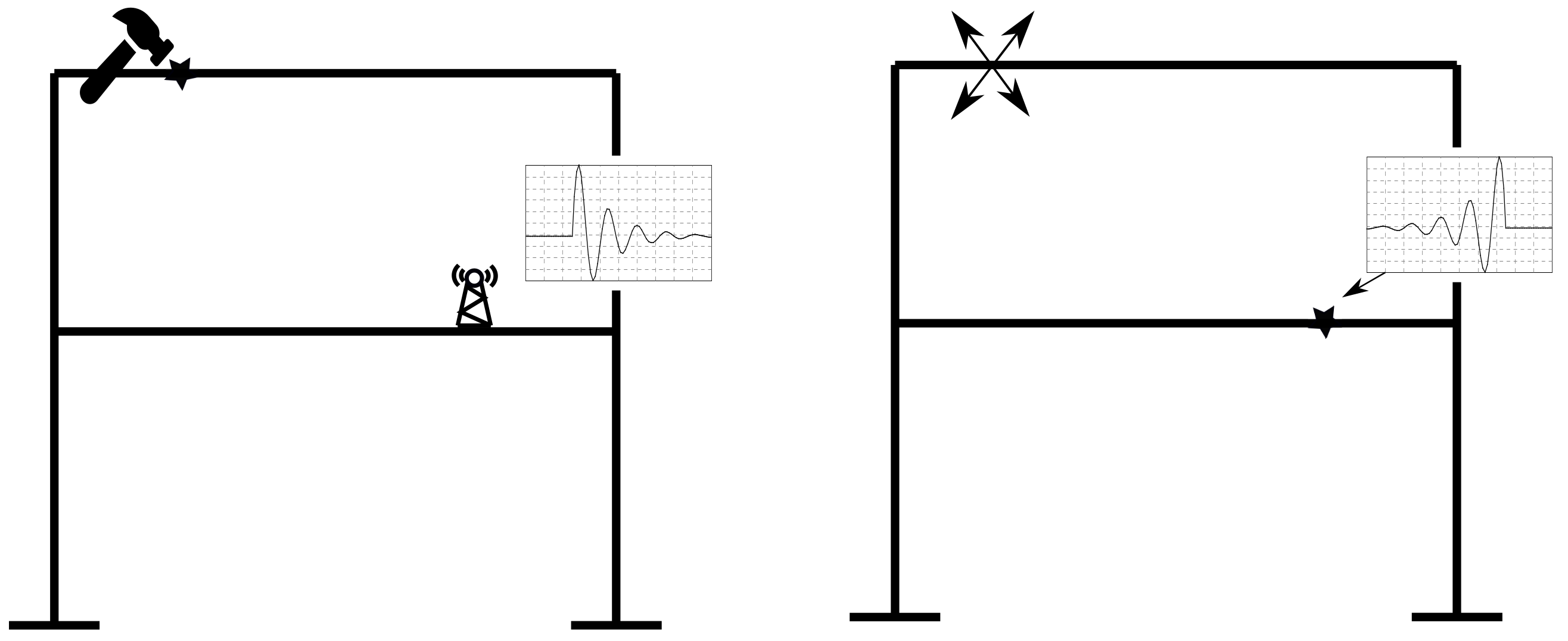
The TR is considered as a two-stage physical process. During the first step, the forward problem takes place when an initial disturbance is such that excites higher frequency motion in the structure which might be seen as axial and/or bending wave propagation phenomena. The second step is the backward one where some quantity of the forward process is reversed in time and re-emitted in the structure. It has been experimentally observed that at the end of this backward process, energy has again been localized at the area where the disturbance originally begun during the forward step [30].

Here, we make an effort to investigate this two-stage procedure through reciprocal statement of linear elastodynamics. We also discuss some different possible ways in order to fire the backward step.

2.2.1. Switching Time Reversal

We choose the ($v,w$) state to be the $\left(v(x,t),u(x,T-t)\right)$. In this case, which is sometimes called a switching time reversal approach [31], the reciprocal statement would be:

$$\begin{array}{cc}\hfill & \underset{0}{\overset{L}{\int }}u(x,t^{*})\ast u(x,t)dx-\underset{0}{\overset{L}{\int }}q(x,t)\ast v(x,t)dx=\hfill \\ \hfill & EI{\left[\frac{{\partial }^{3}u(x,t)}{\partial x^3}\ast v(x,t)-\frac{{\partial }^{2}u(x,t)}{\partial x^2}\ast \frac{\partial v(x,t)}{\partial x}+\frac{\partial u(x,t)}{\partial x}\ast \frac{{\partial }^{2}v(x,t)}{\partial x^2}-u(x,t)\ast \frac{{\partial }^{3}v(x,t)}{\partial x^3}\right]}_0^L\hfill \\ \hfill & +\rho A\underset{0}{\overset{L}{\int }}{\dot{v}}_0\left(x\right)u(x,t)+v_0\left(x\right)\dot{u}(x,t)-{\dot{u}}_0\left(x\right)v(x,t)-u_0\left(x\right)\dot{v}(x,t)dx.\hfill \end{array}$$

(10)

It can be shown that if the forward state is such that produces wave propagation motion originated from a limited range on the spatial x axis of the beam, then a wave refocusing on the same spatial range is expected to take place at the end of the reversed motion in time.

In the case of switching time reversal approaches, based on the reciprocal statement of Equation (10), we expected to observe wave refocusing on the part of the initial disturbance which produced the forward wave propagation motion. Such an approach could lead to interesting time reversal computational tools [32,33]. A usual choice of such a disturbance would be a concentrated impulsive load on point $x_s$ given by $q(x,t)=\delta (x-x_s)\delta \left(t\right)$ resulting in motion $u(x,t)$. In other words, we choose as forward state the one corresponding to the fundamental solution for specific boundary conditions. For the current theoretical approach, this is a good choice, which however could lead to numerical problems and therefore we approximate it with some smoother equivalent. Using the method of eigenmodes, the fundamental solution, also known as Green’s function, is given as:

$$\begin{array}{c}\hfill u(x,t)=\rho A\sum _{n=1}^{\infty }\frac{{\varphi }_n\left(x\right){\varphi }_n\left(x_s\right)}{M_n{\omega }_n}sin{\omega }_{n}t\end{array}$$

(11)

As regards the backward state, it is selected to be the motion $v(x,t)$ produced by a load distribution equal with the reversed in time forward displacement field, that is $w(x,t)=u(x,t^{\ast })$, where $t^{\ast }=T-t$.

After substitution into the reciprocal statement of Equation (10) and some algebraic manipulation we obtain:

$$\begin{array}{c}\hfill v(x_s,t)={\left(\rho A\right)}^2\sum _{n=1}^{\infty }\frac{{\varphi }_n^2\left(x_s\right)}{M_n{\omega }_n^2}\left(sin{\omega }_n(T-t)\ast sin{\omega }_{n}t\right)\end{array}$$

(12)

calculating the time convolution integral we may further write as

$$\begin{array}{c}\hfill v(x_s,t)=-{\left(\rho A\right)}^2\sum _{n=1}^{\infty }\frac{{\varphi }_n^2\left(x_s\right)}{M_n{\omega }_n^2}\frac{sin{\omega }_n(t+T)+sin{\omega }_n(t-T)-2{\omega }_{n}tcos{\omega }_n(t-T)}{4{\omega }_n}\end{array}$$

(13)

which having its maximum value for time $t=T$:

$$\begin{array}{c}\hfill v(x_s,T)=-{\left(\rho A\right)}^2\sum _{n=1}^{\infty }\frac{{\varphi }_n^2\left(x_s\right)}{M_n{\omega }_n^2}\frac{sin2{\omega }_{n}T-2{\omega }_{n}T}{4{\omega }_n},\end{array}$$

(14)

it indicates a refocus on $x_s$ for the time T.

2.2.2. Time Reversed Switched Boundary Conditions

Here, we choose only the boundary conditions state to be the reversed in time switched in space quantity. The swapping of boundary conditions is meant by means of energetically corresponding pairs, that is:

$$\begin{array}{cc}\hfill & v(x,t)\leftrightarrow \frac{{\partial }^{3}v(x,t)}{\partial x^3}\hfill \\ \hfill & \frac{\partial v(x,t)}{\partial x}\leftrightarrow \frac{{\partial }^{2}v(x,t)}{\partial x^2}\hfill \end{array}$$

therefore:

$$\begin{array}{cc}\hfill & \underset{0}{\overset{L}{\int }}w(x,t)\ast u(x,t)dx-\underset{0}{\overset{L}{\int }}q(x,t)\ast v(x,t)dx=\hfill \\ \hfill & EI{\left[\frac{{\partial }^{3}u(x,t)}{\partial x^3}\ast \frac{{\partial }^{3}u(x,t^{\ast })}{\partial x^3}-\frac{{\partial }^{2}u(x,t)}{\partial x^2}\ast \frac{{\partial }^{2}u(x,t^{\ast })}{\partial x^2}+\frac{\partial u(x,t)}{\partial x}\ast \frac{\partial u(x,t^{\ast })}{\partial x}-u(x,t)\ast u(x,t^{*})\right]}_0^L\hfill \\ \hfill & +\rho A\underset{0}{\overset{L}{\int }}{\dot{v}}_0\left(x\right)u(x,t)+v_0\left(x\right)\dot{u}(x,t)-{\dot{u}}_0\left(x\right)v(x,t)-u_0\left(x\right)\dot{v}(x,t)dx.\hfill \end{array}$$

(15)

The proposed procedure can be seen as a generalization of [31,34], where only free surfaces have been studied. A more specific choice of this reciprocal statement would be that of concentrated impulsive load on some point $x_s$ for the forward configuration while for the backward one to assume to be free of excitation loading. Both states are considered to be under silent initial conditions and therefore the reciprocity relation can be written as:

$$\begin{array}{cc}\hfill & v(x_s,t)=\hfill \\ \hfill & EI{\left[\frac{{\partial }^{3}u(x,t)}{\partial x^3}\ast \frac{{\partial }^{3}u(x,t^{\ast })}{\partial x^3}-\frac{{\partial }^{2}u(x,t)}{\partial x^2}\ast \frac{{\partial }^{2}u(x,t^{\ast })}{\partial x^2}+\frac{\partial u(x,t)}{\partial x}\ast \frac{\partial u(x,t^{\ast })}{\partial x}-u(x,t)\ast u(x,t^{\ast })\right]}_0^L\hfill \end{array}$$

(16)

In this case, we can not take advantage of modes’ orthogonality; however, the terms of the form of Equation (13) existing here are also dominating resulting in a maximum value of $v(x_s,t)$ at time $t=T$ with a refocusing of the wave field on the point $x_s$.

3. Computational Time Reversal for Structures

In computational TR, at least one of the two steps, that is forward or backward step, is to be done numerically using some appropriate method, e.g., finite element method (FEM) or boundary element method (BEM). Here, we use the conventional FEM, used in the majority of structural dynamics problems, realizing the switched TR described in Section 2.2.1. However, it is worth mentioning that in specific cases, it could be that BEM would be the natural choice [35] for utilizing the TR approach described in Section 2.2.2.

The methodology could be stated as described in Figure 1. We assume, in the forward step, that a source excites on some point $x_s$ the structure and that the response $u_r\left(t\right)$ is recorded on some other point $x_r$ for the time duration T. Then, in the backward step, the reversed in time response’s signal $u_r(T-t)$ is re-emitted as excitation on the $x_r$ point. In that backward step, an energy refocusing will appear on the $x_s$ point after the same duration of time T. This main application is called a source localization approach. Another application is that of damage detection which considers damage location $x_d$ as the point of a secondary source. This secondary excitation equals the signal scattered by the presence of the damage and could be given in relation to the original incident field emitted by the source at $x_r$ as

$$\begin{array}{c}\hfill u_r^d=u_r^t-u_r\end{array}$$

(17)

in other words, $u_r^t$ contains both primal and secondary source influence on response, $u_r$ only that of the original one and $u_r^d$ that of damage scattered field. Therefore, by re-emitting (in the backward step) the signal reversed in time $u_r$, one could locate the original source; by re-emitting $u_r^d$, one could locate the secondary source due to damage; and finally, by $u_r^t$ re-emission, one could locate both the original and secondary sources.

3.1. Standard Forward Step

For a time interval of interest T, the finite element model of a system of N DOFs under transient dynamic conditions will be governed by equations of motion:

$$\begin{array}{c}\hfill \mathbf{M}\ddot{\mathbf{u}}\left(t\right)+\mathbf{C}\dot{\mathbf{u}}\left(t\right)+\mathbf{K}\mathbf{u}\left(t\right)=f\left(t\right)\mathbf{f}\end{array}$$

(18)

where $\mathbf{f}$ is a load vector usually containing unit values for the components corresponding to degrees of freedom acting as probes or otherwise zeros. Furthermore, $\mathbf{K}$ is the standard stiffness matrix, $\mathbf{M}$ the mass matrix and $\mathbf{C}$ the matrix for the damping. Temporal function $f\left(t\right)$ might be given as a Ricker pulse of the form:

$$\begin{array}{c}\hfill f\left(t\right)=\left(1-2{\pi }^2{s}^2{(t-t_0)}^2\right)e^{-{\pi }^2{s}^2{(t-t_0)}^2}\end{array}$$

(19)

We assume a subset of the system’s DOFs, ${\mathbf{u}}_{\mathbf{r}}\subseteq \mathbf{u}$, where data acquisition takes place by recording the time history of response.

3.2. The Time Reversal or Backward Step

The time histories for recorded DOFs ${\mathbf{u}}_{\mathbf{r}}$ are time-reversed and retransmitted into the medium as excitation (sources).

$$\begin{array}{c}\hfill \mathbf{M}\ddot{\widehat{\mathbf{u}}}\left(t\right)+\mathbf{C}\dot{\widehat{\mathbf{u}}}\left(t\right)+\mathbf{K}\widehat{\mathbf{u}}\left(t\right)=\widehat{f}\left(t\right)\widehat{\mathbf{f}}\end{array}$$

(20)

Following previous work [33,36], our choice here is to assume $\widehat{\mathbf{f}}$ of zero values components or units when it corresponds to some ${\mathbf{u}}_{\mathbf{r}}$ component. Evolution $\widehat{f}\left(t\right)=u\left(t^{\ast }\right)$ is the reversed in time component of vector $\mathbf{u}$, actually being the solution of the forward problem of Equation (18). For the case of structural irregularities, i.e., damage localization, ${\mathbf{u}}_{\mathbf{r}}$ contains the scattered field response.

Of crucial importance is the choice of quantity to be monitored in order to observe refocusing during the backward step. Such refocusing on appropriate discrete time step [33] or time averaged [37] will indicate the spatial location of original source point of the forward step. As for monitoring quantity, we consider here the value of some DOF, its time derivative, some appropriate norm (e.g., Euclidean) or even some energetic quantity, as would be the density of elastic, kinetic or total energy.

3.3. Signal-to-Noise Ratio

One of main objectives of this work was the investigation of the signal-to-noise ratio (SNR) for various receivers’ placement scenarios. Signal-to-noise ratio is a quantity of paramount importance, defined as the value of the image at the true source location divided by the noise, defined here as the maximal value of the image outside a region around the true source location. The parametric study of SNR can give us a directive on the amount of receivers we should need for imaging. Furthermore, it has been found to be very instructive for investigating the optimal sensors’ placement together with the quantity we should monitor on each location. For that purpose, two parametric studies have been done, in one-dimensional beam and two-dimensional frame structure.

3.4. Illustrative Comparison

We present here the results for a common setup by utilizing both approaches that arise from Section 2.2.1 and Section 2.2.2. These TR approaches fulfil the partial information property [38]. We consider a simply supported beam of length L. During the forward step, excitation loading acts as a source on the $0.65$ L point in the form of a Ricker pulse of Equation (19) both in the transverse and axial direction. Our selection of the monitoring quantity is that of the total energy density.

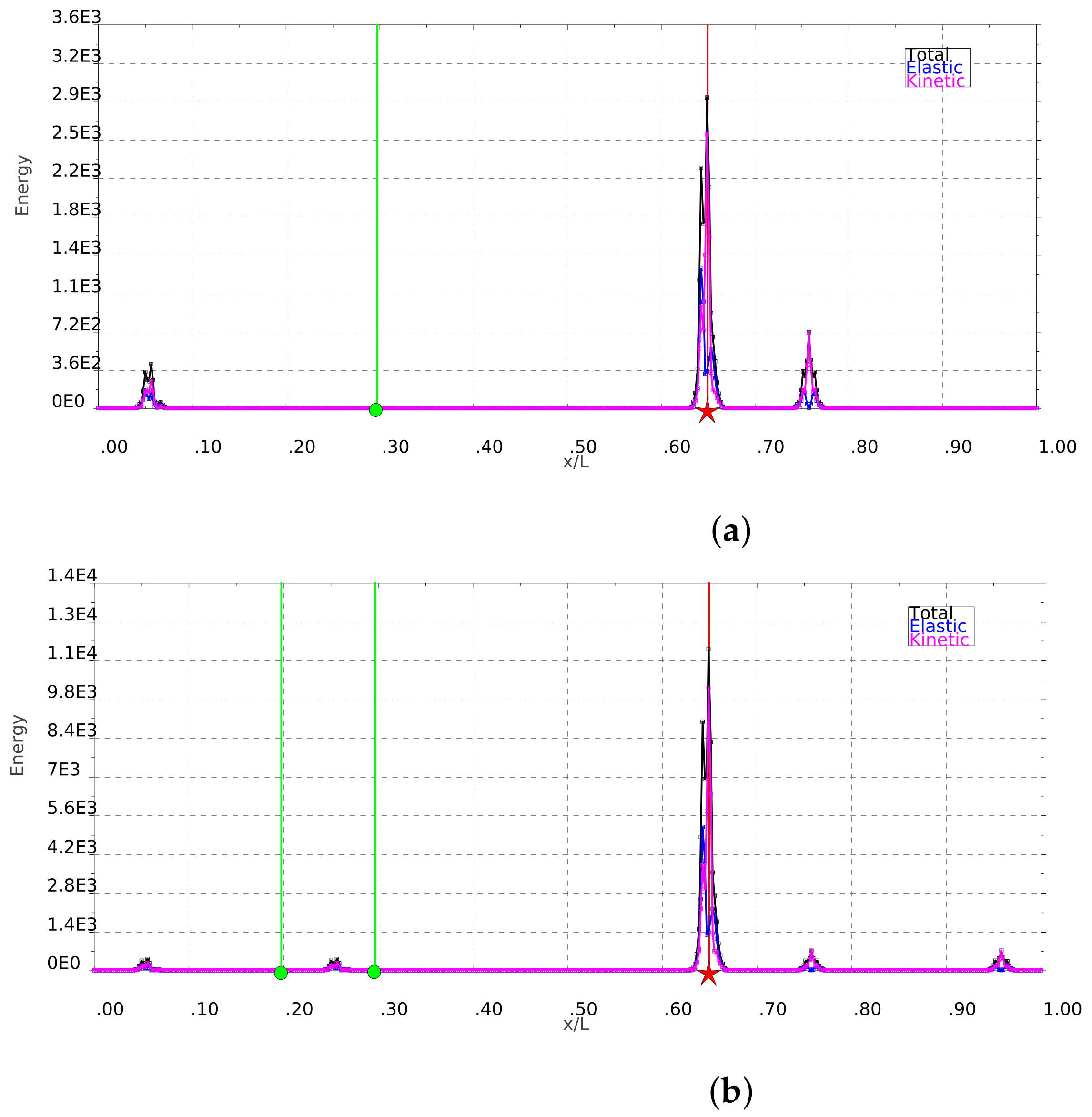
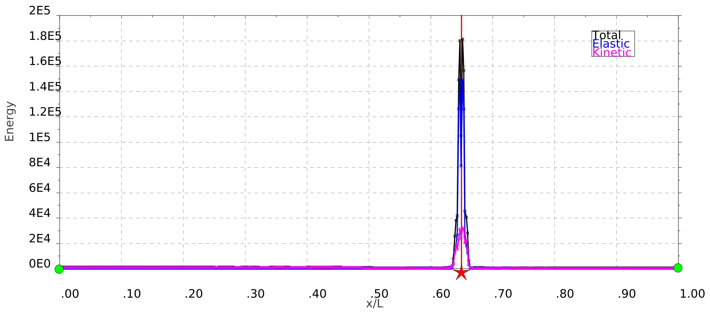
As it can be observed in plots of Figure 2 together with the original point of source at $0.65$ L, two other smaller peaks (ghosts) are present. The ratio of the peak at the original source location to the ghosts’ peaks is increased with the increasing number of receivers. The presence of ghosts is due to the bounded range of the domain and their location depends on the location of the receiver and boundary conditions. An in depth investigation has been presented in the literature [36] for the case of the acoustic field. In the current work, in the following section we present further results for the case of a beam and frame structures. Furthermore, in the plot of Figure 3, similar results for this specific example are presented for the switched boundary conditions’ time reversal, presented in Section 2.2.2, with very satisfactory results in the absence of ghosts. However, the TR of Section 2.2.1 is a better choice since it is fully adaptive with possible unlimited SNR improvement.

4. Applications with Numerical Examples

The proposed technique has been used for the study of a couple of rather academic numerical examples and their solutions have been implemented in a Java open source framework for calculations [39]. The first one is related to an one-dimensional beam. A two dimensional frame structure, which is a common structure in various applications, is studied in the second example. It should be emphasized that the present feasibility study considers academic examples including the material properties, which do not represent specific real structures or materials. In particular, a standard approach in acoustics considering unit values for both the elasticity modulus and density is followed here, resulting in unit wave propagation velocity for axial waves.

4.1. Energy Refocusing

A very interesting application of TR that could be seen as a structural active control procedure is that of energy refocusing [34]. This application switches the usual implementation of TR where the forward step is assumed to be the one realized physically as the data acquisition procedure and the backward one to be the one to be held numerically. As an energy refocusing example, the issue could be stated as: find the excitation to be imposed on a limited number of specific locations of the structure, such that the energy to be focused on some particular location of the structure in a controlled manner and in a well-approximated time. In order to succeed, the forward problem is numerically solved on a digital twin of the structure, by exciting some source location and the response on a limited number of spatial points and selected DOFs for a time duration T is collected. Afterwards, the structure is stimulated by exciting the selected DOFs on the specific locations by imposing loads as the time reversed collected response data and expected the energy to be refocused on the original source location after the passage of time equal to the original forward procedure duration T. The intelligent usage of this concept, for instance, with the help of remote sensors and actuators, will enhance the performance of structural health monitoring systems.

4.2. Source Localization

In contrast to the TR application presented in Section 4.1, here, we return to a more usual application, that of source localization. Here, we assume that the forward step might be held physically in the process of which response data is collected in a limited number of DOFs on specific spatial locations. Then, we may take advantage of these data since by numerically solving the backward step, we may redefine the original spatial location of the source.

4.2.1. One-Dimensional Beam

In this section, the 1D beam is analysed and the results of the source localization are presented. During the forward process, an excitation source located at point $x_s$ and three receivers, equidistantly distributed along the medium at $L/3,2L/3$ and at the end of the free edge, collect the data.

For the calculations of the academic example presented here, a one-dimensional beam with a length L = 30 m, mass density $\rho$ = 1 kg/m³, modulus of elasticity E = 1 Pa and Poisson’s ratio $\nu$ = 0.25. Moreover, the total experiment’s duration was T = $t_o$+$\frac{2L}{c_1}$ = 63 s, where the initial time is $t_o$ = 3 s, the number of discrete time steps is chosen as a power of two ($2^{12}$) and the mesh is the 1950 finite elements which means a distance between nodes $dx$ = 0.015 m and a time step $dt$ = 0.015 s.

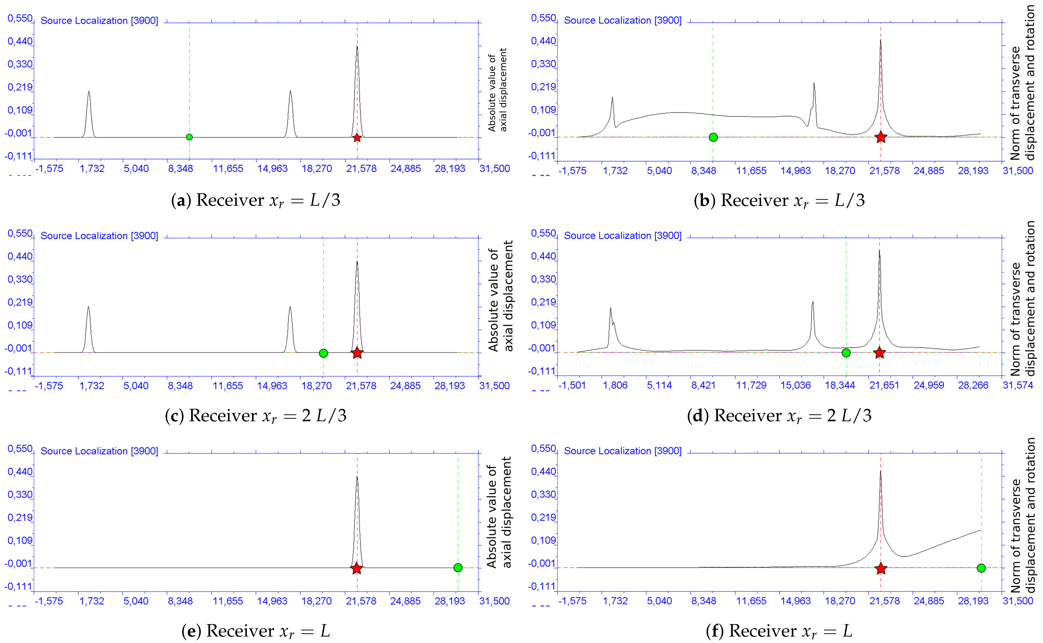
During the forward process, we assume three receivers, along the axis of the beam, collecting data for displacements and/or velocities for every DOF of nodes. The backward step problem is numerically solved again for each receiver. The receiver now acts as a source point that emits the recorded signal reversed in time as loading. Refocusing the wave at the source point $x_s$ takes place at time $T-t_0$ = 60 s. Plots of Figure 4 depict the Euclidean norm of displacements at the specific discrete time step $N_t-\frac{t_0}{dt}$ = 3900. It is important to mention that secondary peaks are presented because of the existence of the boundaries. These peaks are also responsible for the noise created because the domain is bounded and waves are reflected back. The exact location of these secondary peaks depends on the relative position of receivers. This fact acts beneficially on the SNR improvement using multiple receivers distributed on the body of some structure, as it will be shown later in a following section.

4.2.2. Two-Dimensional Frame Structure

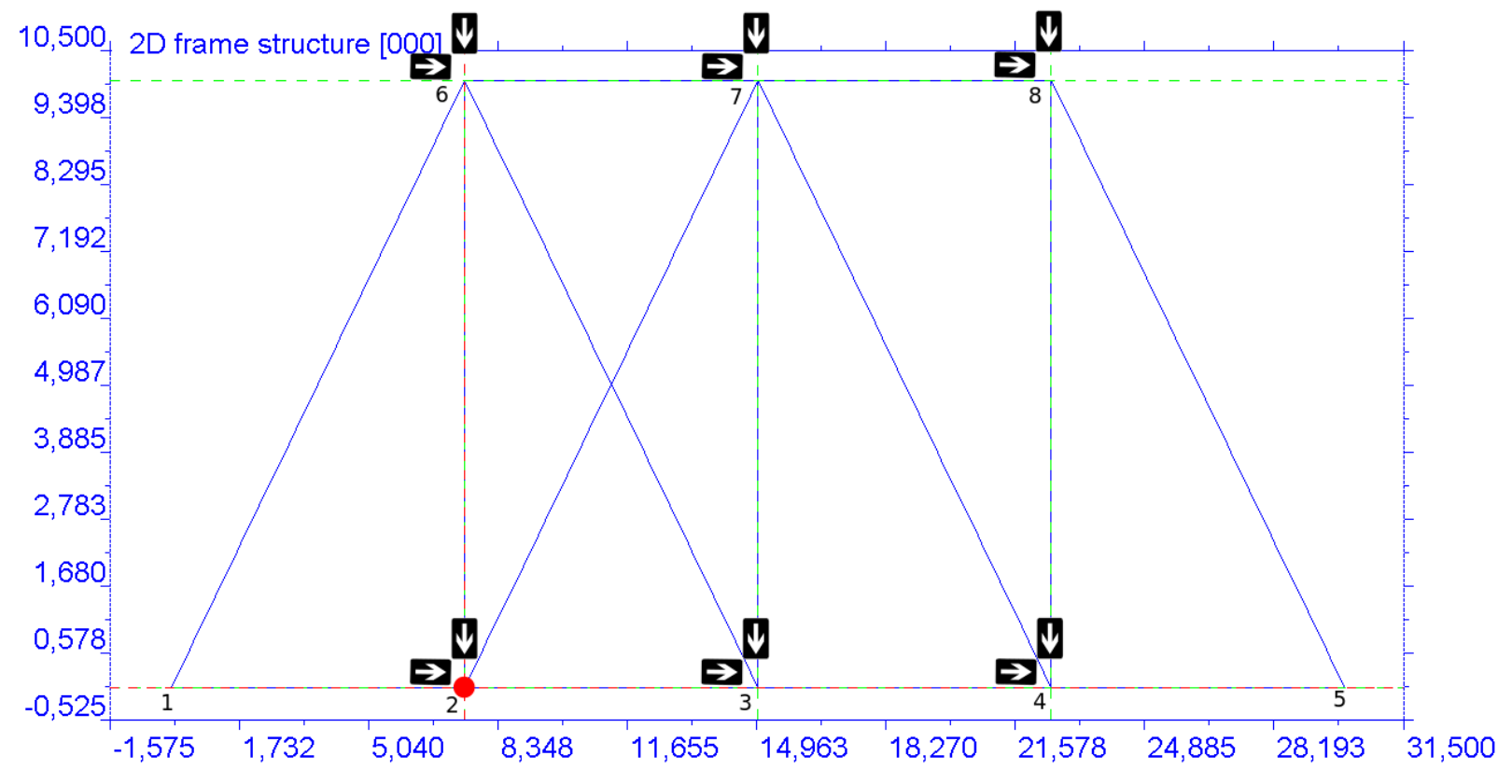
In order to demonstrate the applicability of the method to more complicated geometries, a 2D frame structure made of an assembly of beams is studied (see Figure 5). The structure is assumed to be of a total length L = 30 mm while the height is H = 10 m. The modulus of elasticity was chosen E = $1Pa$, the mass density $\rho$ = 1 kg/m³ and the Poisson’s ratio $\nu$ = 0.25. The total duration of the numerical experiment for T =$t_o$$+\frac{2L}{c_1}$ = 63 s, where the initial time is $t_o$ = 3 s when the source is imposed as a pulse, the number of discrete time steps is chosen as a power of two $2^{11}$ and the number of elements for every beam between the main nodes is 200, which means a total number of 2800 finite elements.

During the forward procedure, six receivers are used to collect the response data (displacements and velocities) for every DOF (two translational and one rotational). In Figure 5, the possible positions of sensors are indicated together with the respective recording directions for every receiver. There is one single excitation point on the node of ID = 2 at the bottom horizontal part of the assembly. The leftmost and rightmost nodes are restrained in zero horizontal and vertical displacement.

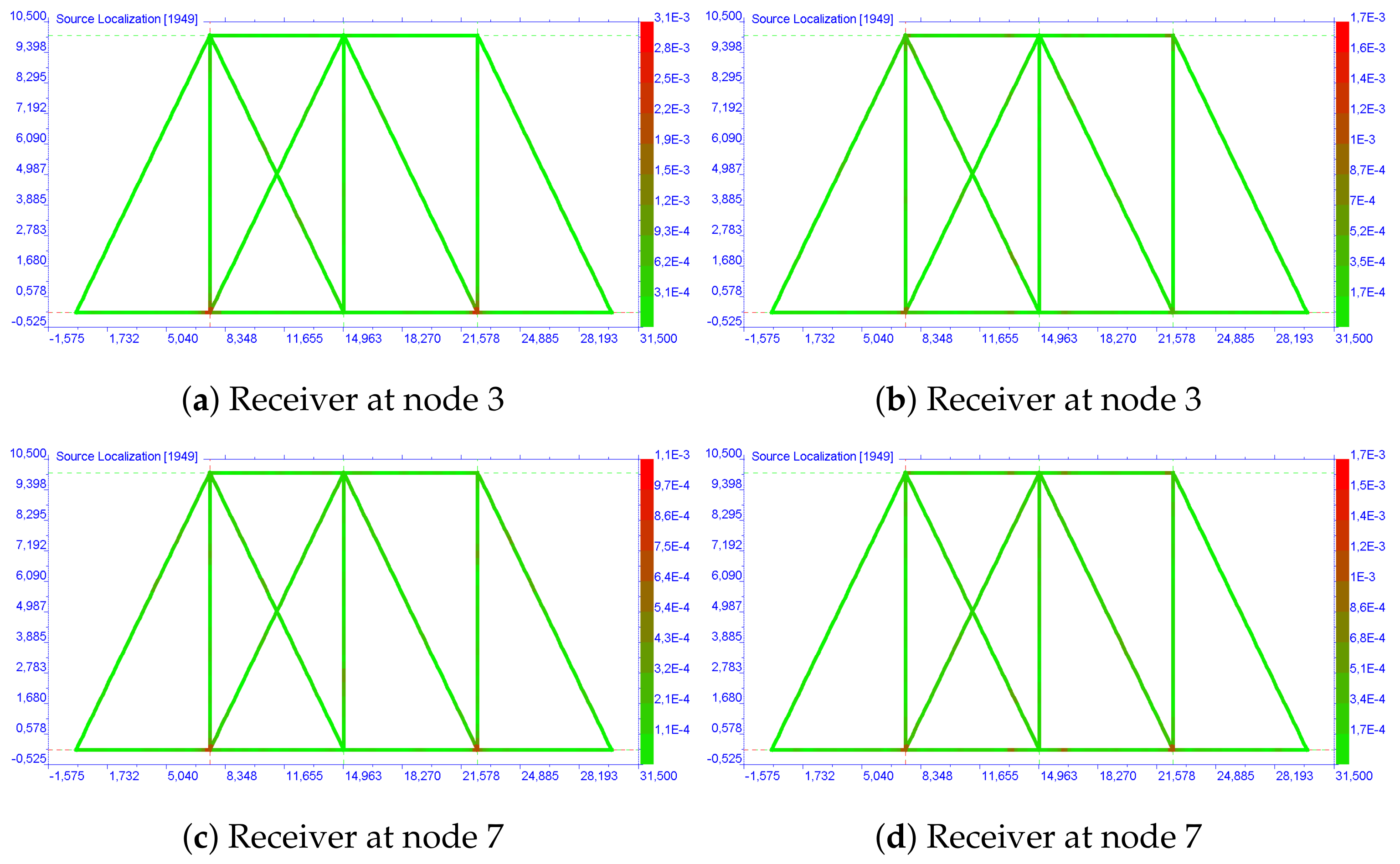
For the backward step, the time when the wave refocuses on the excitation point is T − $t_0$ = 60 s, that is the $t_r$ = 1949 discrete time step. In the plots of Figure 6, the Euclidean norm of displacements, with respective units, is shown for the $t_r$ time step. While in the plot of Figure 6b, one may observe that ghost refocused signals are not so strong, in the rest of the plots of Figure 6, there is an obvious appearance of a symmetric-like ghost on node 4 with the value of the same order. Furthermore, we considered a 10% level of Gaussian noise in the recorded signals of displacement, and observed that the location of the source can be similarly well reconstructed.

4.3. Optimal Placement of Sensors

In this section, the SNR for both the one-dimensional beam and the 2D frame structure is studied. The framework is the same for both configurations with the previously presented examples. A fixed set of possible receivers is initially assumed, each of them defined by the spatial location and the monitored DOF. The first initial receiver is chosen, to check for the SNR obtained using some specific monitored quantity. Then, the number of receivers is gradually increased, randomly chosen from the fixed set of possible ones, and the SNR is tracked. This way one is able to observe the influence of the increasing number of receivers on the SNR and to choose the optimal placement of receivers for a specific number of sensors in order to optimize the structural health monitoring system for a certain SNR measure.

4.3.1. One-Dimensional Beam

For the one-dimensional beam case, we studied sets of receivers chosen from a maximum number of 12 possible equidistant receivers. Starting from a single receiver, then the number is gradually increased by one, randomly chosen by the set from the fixed possible 12 sensors. Results for the SNR are shown in Figure 7 where it is obvious that an increasing number of receivers SNR is improved (increased). The plots indicate an almost linear relation with respect to the receivers’ number with deviations that occurred because of ghost superposition or cancellation. For the case of axial motion, the case of the left plot in Figure 7a, the factor of the linear evolution with the number of receivers is that of two as it was expected [36], while in the case of transverse and rotational motion depicted in the plot of Figure 7b, the corresponding coefficient is smaller.

4.3.2. Two-Dimensional Frame Structure

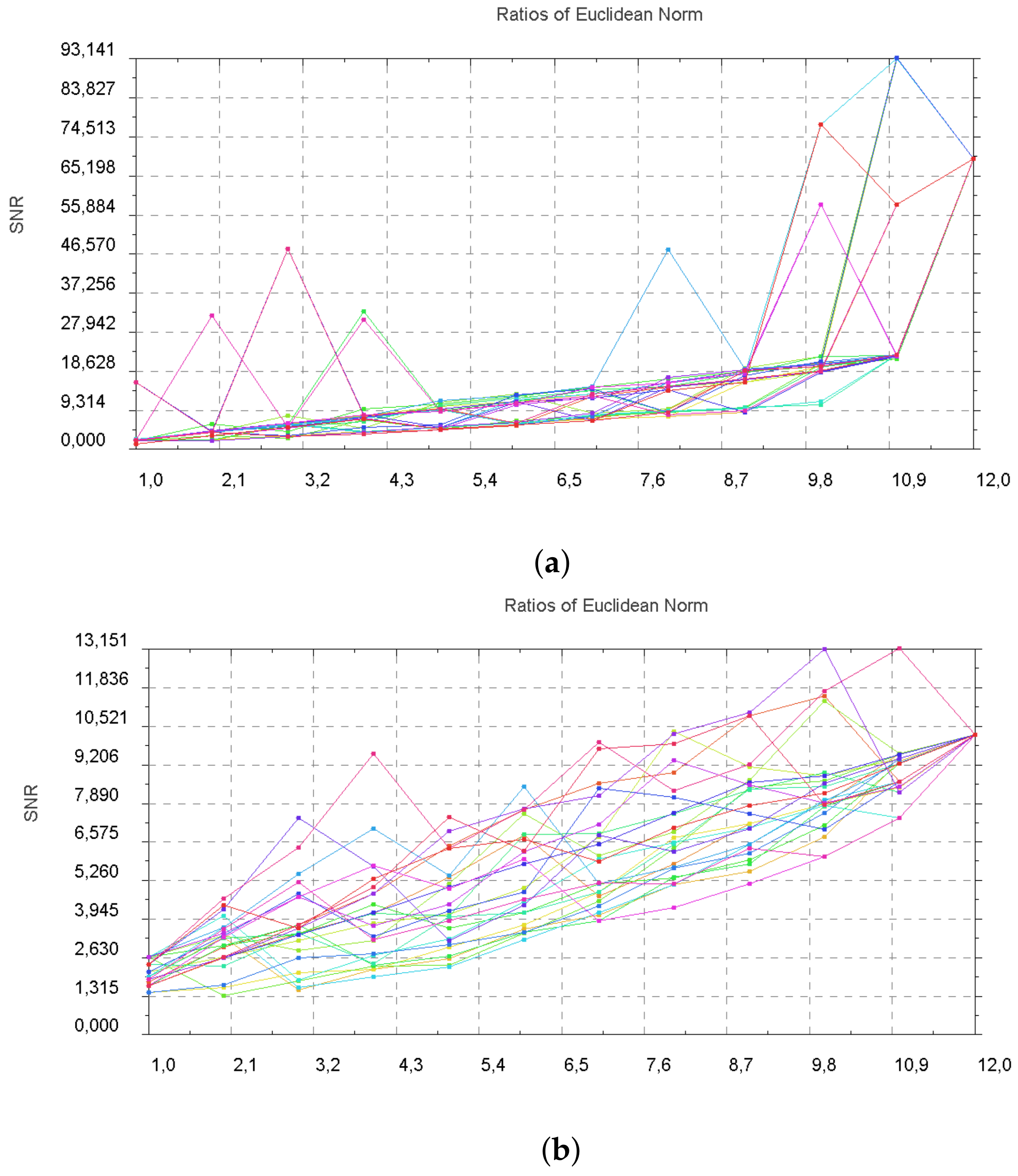
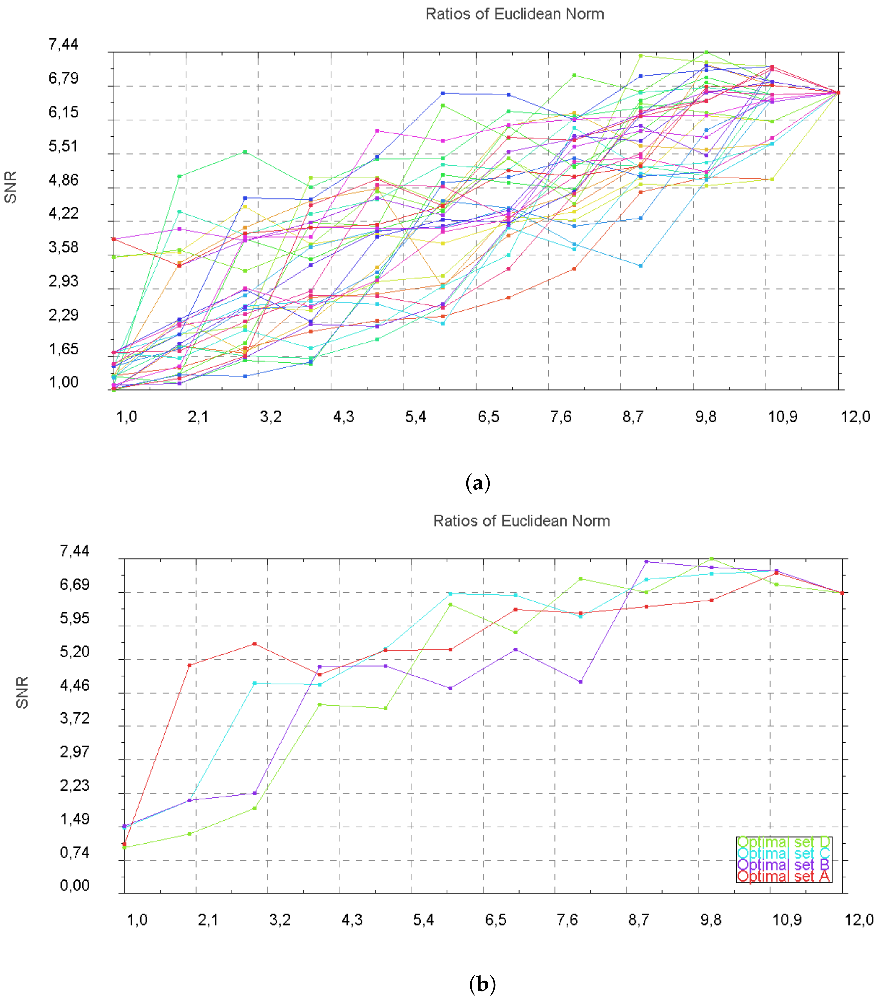
In the case of the 2D beam assembly, the 12 possible positions and monitored DOFs are shown in Figure 5. The main aim of this investigation was to define the optimal set of receivers from the available fixed number of 12 existing sensors. Figure 8a shows the SNR for 31 random receiver sets. SNR is defined as the ratio of the max peak value at the source point and the next max peak value, less than the global maximum one. In order to determine the optimal solution for a specific number of receivers, the higher SNR is chosen from Figure 8a at the abscissa corresponding to that number of receivers. In

Table 1. Optimal receiver set.

	Original Signals					Noise Considered
# Recs/Opt.set	$\mathbf{A}$	$\mathbf{B}$	$\mathbf{C}$	$\mathbf{D}$	$\mathbf{B}$	$\mathbf{A}$	$\mathbf{B}$	$\mathbf{C}$	$\mathbf{D}$	$\mathbf{D}$
2	$y_3,y_2$					$y_8,y_2$
4	$y_3,y_2$	$y_8,x_8$				$x_8,y_6$	$y_8,y_2$
6	$x_8,y_4$	$y_3,y_2$	$x_6,x_2$			$y_6,x_8$	$x_2,x_7$	$y_2,y_8$
8	$x_3,y_4$	$x_6,y_8$	$x_4,y_2$	$y_6,x_2$		$x_3,y_4$	$y_7,x_2$	$y_8,y_2$	$x_8,y_6$
10	$y_3,y_2$	$y_8,x_8$	$x_7,y_6$	$x_4,x_2$	$y_7,x_6$	$x_3,y_4$	$y_7,x_2$	$y_8,y_2$	$x_8,y_6$	$x_6,y_3$

(original signals), one may observe that for 4 ($y_3,y_2,y_8,x_8$) and 10 ($y_3,y_2,y_8,x_8,x_7,y_6,x_4,x_2,y_7,x_6$) receivers, the optimal solution belongs to the same receiver set (see Figure 8b, optimal set B). Moreover, the receiver sets for two, six and eight receivers are different, as shown in Figure 8b as the optimal sets A, C and D, respectively.

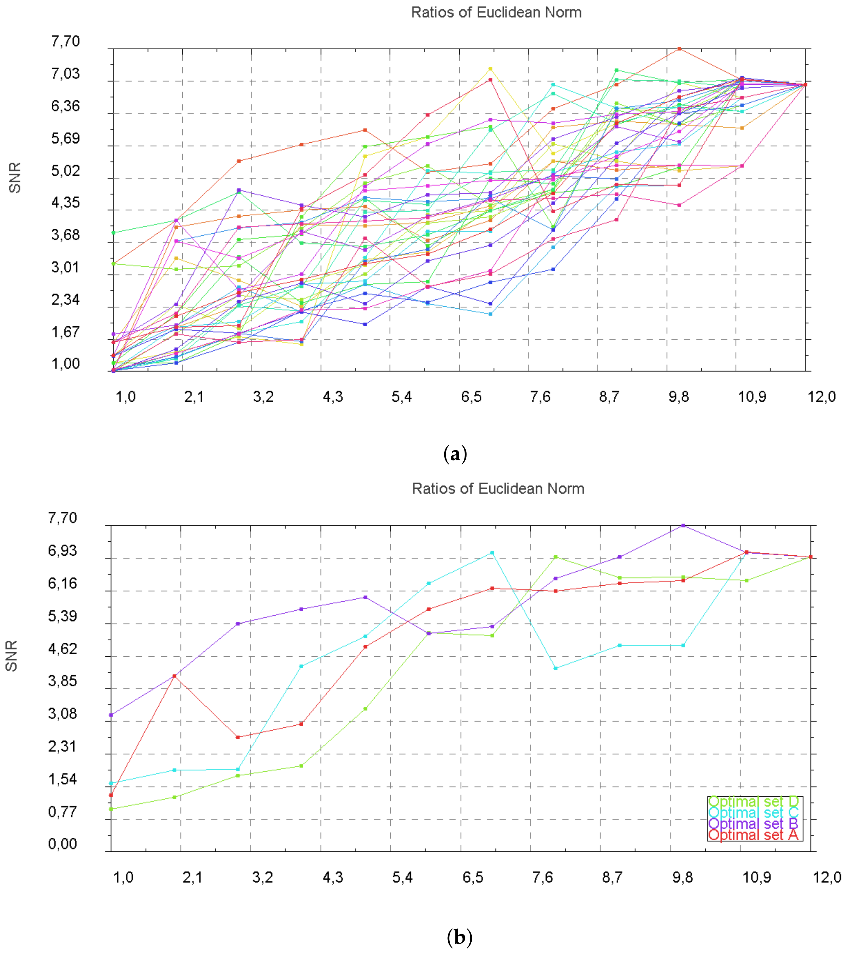
Considering Gaussian noise, optimal receiver sets for various numbers of sensors differ from each other, except for the scenarios with 8 and 10 receivers. In Figure 9a, the SNR is plotted after randomly placing 31 receiver sets. Specifically, in Table 1 (noise considered), the optimal receiver sets for various numbers of sensors are shown. In Figure 9b, the SNR evolution with consecutive placement of receivers for these optimal sets is depicted.

4.4. Damage Identification

4.4.1. One-Dimensional Beam

In this section, a small damaged area is assumed on the beam, from $x_1$ = $0.1795$L to $x_1$ = $0.18$L where the modulus of elasticity $E_{sc}$ = $0.2$ for the material and the cross-section $A_{sc}$ = $0.5$ are reduced. The corresponding reduced wave speed on that altered area is $c_{sc,1}$ = $0.2$ m/s. For that controlled numerical experiment, it is possible to estimate or even with accuracy, calculate the time needed for the incident field to reach the scatterer. The source pulse is emitted at $0.75$ L and the first damaged boundary is at $0.18$ L, the distance between these nodes is $0.57$ L = $17.1$ m. The wave speed for axial waves is $c_1$ = 1 m/s, therefore a time t = $17.1$ s. The time $t_{sc}^a$ that the damaged area acts as a source (scattered field) because of the damage corresponds to the time when the axial wave, originally created at time $t_0$ because of the primal source, approaches the damaged area. Therefore, the corresponding refocusing time during the backward step is $T-(t_{sc}^a+t_0)$, where T is the total duration of forward process. Similarly, the refocusing time for transverse waves is $T-(t_{sc}^b+t_0)$, with $t^b$ the time needed for bending waves initiated from the source to approach the damaged area. The plots of Figure 10 illustrate refocusing cases considering different receivers as well as distinguishing the case when axial or bending waves are examined. As it can be observed, the identification and location of the damage on the beam for almost any selection of receiver and wave monitoring (DOF type) is possible. The exception seems to be the case of Figure 10f, which is intentionally presented here, in order to mention the reason that is the limited duration time of the experiment. Bending waves initiated from the secondary source at the damage area do not have the necessary time to approach the rightmost receiver, also keeping in mind the initial time $t_0$ and the time $t_{sc}^b$ needed for the primal wave to approach the damage area and fire the secondary wave emission.

4.4.2. Two-Dimensional Frame Structure

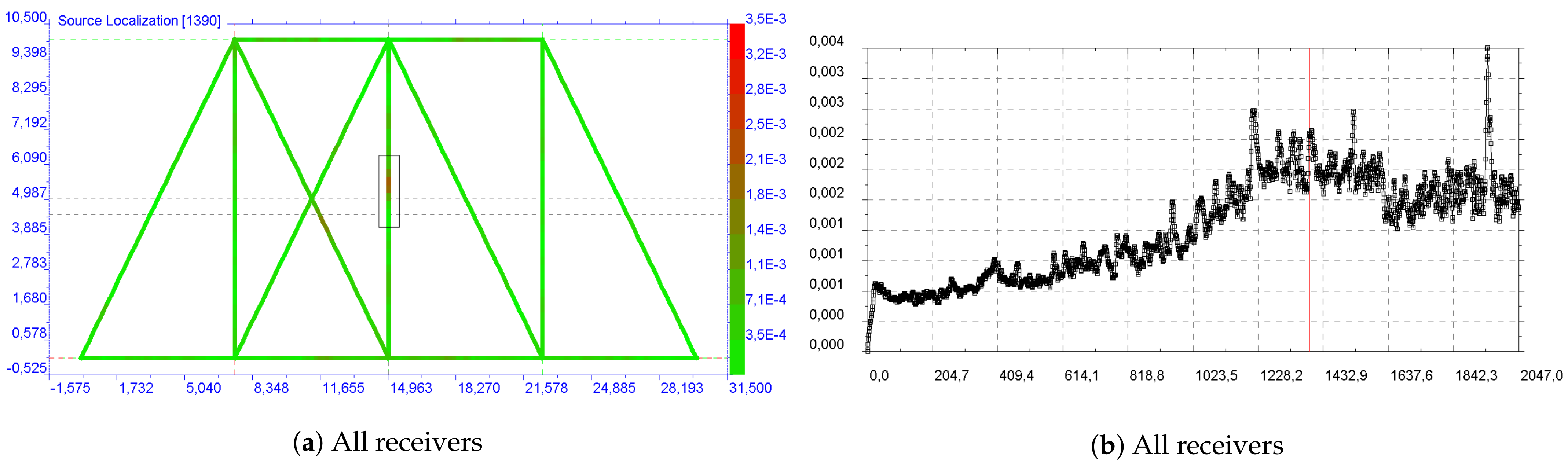
Some preliminary results from an ongoing study are presented for the case of some scatter, i.e., damage, in a two-dimensional frame. To be more specific, damage is assumed to be located at some small area ranging 10 nodes (nine finite elements), located from $(15.0,4.5)$ to $(15.0,5.0)$ (see Figure 5). Moreover, the mechanical features of this area is the material’s modulus of elasticity $E_{sc}$ = $\frac{E}{5}$ = $0.2$ and the cross-section $A_{sc}$ = $\frac{A}{2}$ = $0.5$. These values result an important reduction in wave velocities within the damaged area. The time for which the wave reaches the damaged area is estimated to be between 655 and 670 time steps. As a result, because of time reversibility, the expected discrete refocusing time range turns out from the subtraction of $N_t$ = $2^{11}$ resulting a time step range between 1378 and 1393. In Figure 11 (left) it can be observed that in the discrete imaging time step 1373, there is a bright red colour near the scattered area. In Figure 11 (right), the evolution in time of the maximum value of the monitored variable is plotted, which may serve as an indicator for defining the appropriate time step for the reconstruction of refocusing. It was mentioned here that one should further critically consider both the selection of the most appropriate monitored variable (displacement, velocity, energy based, etc.) as well as the most proper tracker of that imaging variable’s norm evolution in time (maximum value of Euclidean norm, Shannon entropy, etc.).

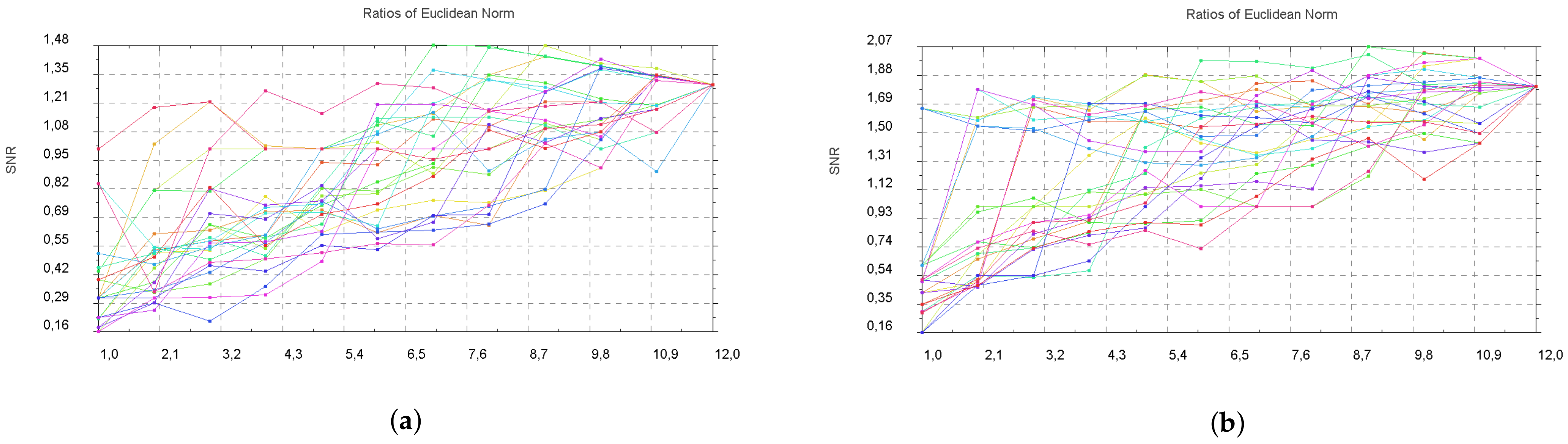
Figure 12 presents the SNR for 25 random receiver sets. It is worth mentioning that SNR has an almost linear attitude both for displacements or velocities as monitored variables. However, there is a considerable focused signal in the damage area when more than eight or nine receivers are used. As a result, here the ratio is always calculated using the value of the monitored variable in the damage area divided by the maximal value outside this area. Figure 12 (right) indicates that nine receivers are required in order to identify the defect. For this reason, if less than nine receivers are used, the SNR is lower than 1.

4.5. Imaging in Frequency Domain

Imaging techniques traditionally take place in the frequency domain. By this, one avoids the need to establish the appropriate time step of a refocusing snapshot. The imaging functional for our case is given as [33]:

$$I_m=\frac{1}{2\pi }\sum _{\omega }\sum _{r=1}^{N_r}\overline{{\widehat{h}}_{rs}\left(\omega \right){\widehat{f}}_s\left(\omega \right)}{\widehat{h}}_{rm}\left(\omega \right)=\frac{1}{2\pi }\sum _{\omega }\sum _{r=1}^{N_r}\overline{{\widehat{u}}_r\left(\omega \right)}{\widehat{h}}_{rm}\left(\omega \right)$$

(21)

which associates a value at the $m^{\mathrm{th}}$ DOF by back propagating the recordings (data) reversed in time, $\overline{{\widehat{u}}_r\left(\omega \right)}$, using all receivers and all available frequencies. For problems of damage localization in the frequency domain, the scattered field at the receivers are considered and the imaging functional is defined as (mention here that a typo originally existed in the respective equation of chapter [33] has been corrected here in Equation (22)):

$$I_m=\sum _{\omega }\sum _{r=1}^{N_r}\overline{{\widehat{u}}_{rs}^{\mathrm{sc}}\left(\omega \right)}{\widehat{h}}_{rm}\left(\omega \right){\widehat{h}}_{ms}\left(\omega \right),$$

(22)

where ${\widehat{u}}_{rs}^{\mathrm{sc}}\left(\omega \right)$ is the scattered field recorded at rth DOF due to an excitation at the $s^{\mathrm{th}}$ DOF.

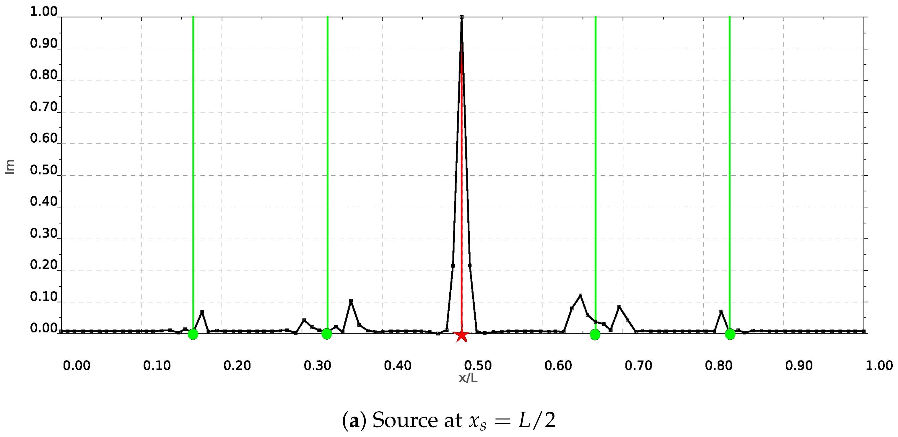
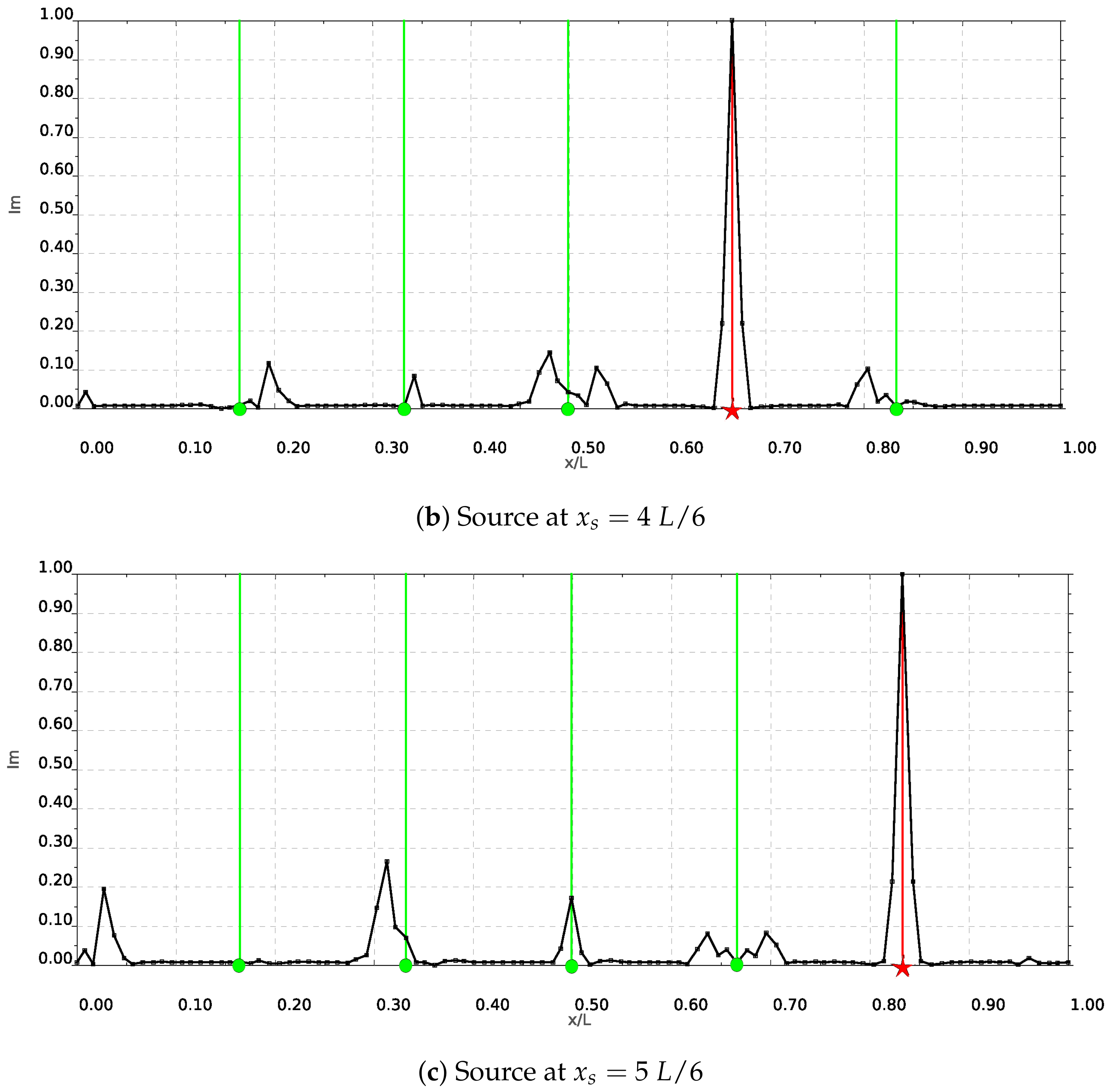
A numerical example based on the same setup as that of Section 3.4 is presented for the general case of source localization based on Equation (21). To the best of the authors’ knowledge, such an implementation for the case of beam bending has not been published in the literature to date. Similar implementation was first presented in [40] for the case of an 1D acoustic field or for the axial deformation of a rod. It has been assumed that there exist five equidistant stations on the beam that may operate as the source and/or receiver points to emit signals in the form of Ricker pulses and/or record the response data of beams’ transverse displacements. The experiment has been conducted numerically, using 480 nodes with a respective number of finite elements. For the spatial locations where values for imaging are to be defined, 103 points have been considered including the two boundaries. The results for imaging where source localization is performed using Equation (21) are depicted in plots of Figure 13 for several source locations, each time using the same number of receivers.

5. Conclusions

The time reversal method has been used for the study of structural health monitoring problems with beam and frame structures. The method is based on solid theoretical investigations in the area of wave propagation in continuous media and must be specialized for classes of structures. Beams and two-dimensional frames are studied here, since these are the most common elements in structural analysis. Future investigations may consider three-dimensional frame structures and plates or shells.

TR is based on the time reversibility of the wave equation. In theory, if all output signals can be measured and fed, after reversion, onto the structure, the resulting wave will refocus on loading sources or damages and other defects. In practice, the measurement and utilization of all output signals is impossible due to technological and resource limitations. Therefore, the practical question arises where to put measurement devices, how many of them and which DOFs one should capture. These questions must be replied for every specific class of structures, like trusses, frames, plates etc. This justifies the numerical investigation reported in this paper. On top of that, the structure can not be isolated from the environment and parasitic reflections from boundaries or structural elements away from the area of investigation appear. These parasitic parts of data are characterized as noise. The influence of the signal to noise ratio on the effectiveness of the method was the second task of our investigation.

The numerical experiments reported here have demonstrated that the source and damage identification is possible based on TR technique. The investigation has been based on unit values of elasticity and cross-section constants. The application of real data is straightforward.

The applicability of the method to a specific structure and task requires the careful consideration of several parameters indicated in the present study, such as the number and placement of the sensors and the quantities to be measured and used. Furthermore, a BEM time reversal implementation utilizing time reversed boundary conditions, which may be of interest for certain applications, is under consideration. For practical applications, signal and measurement errors as well as the existence of stochastically distributed material parameters, must be investigated. Furthermore, an experimental verification is planned. All these aspects are left for future research and development work.

References

- Stavroulakis, G.E. Inverse and Crac Identification Problems in Engineering Mechanics; Springer Science & Business Media: Berlin/Heidelberg, Germany, 2000. [Google Scholar]
- Mróz, Z.; Stavroulakis, G.E. (Eds.) Parameter Identification of Materials and Structures; Springer Science & Business Media: Berlin/Heidelberg, Germany, 2007; Volume 469. [Google Scholar]
- Psychas, I.D.; Schauer, M.; Böhrnsen, J.U.; Marinaki, M.; Marinakis, Y.; Langer, S.C.; Stavroulakis, G.E. Detection of defective pile geometries using a coupled FEM/SBFEM approach and an ant colony classification algorithm. Acta Mech. 2016, 227, 1279–1291. [Google Scholar] [CrossRef]
- Protopapadakis, E.; Schauer, M.; Pierri, E.; Doulamis, A.D.; Stavroulakis, G.E.; Böhrnsen, J.U.; Langer, S. A genetically optimized neural classifier applied to numerical pile integrity tests considering concrete piles. Comput. Struct. 2016, 162, 68–79. [Google Scholar] [CrossRef]
- Prada, C.; Wu, F.; Fink, M. The iterative time reversal mirror: A solution to self-focusing in the pulse echo mode. J. Acoust. Soc. Am. 1991, 90, 1119–1129. [Google Scholar] [CrossRef]
- Bardos, C. The Time reversal method according to Mathias Fink. In Inverse Problems, Boundary Control, Integral Geometry and Related Topics; Ugra Research Institute of Information Technologies: Khanty-Mansiysk, Russia, 2005. [Google Scholar]
- Antes, H. Anwendungen der Methode der Randelemente in der Elastodynamik und der Fluiddynamik; B.G. Teubner: Stuttgart, Germany, 1988. [Google Scholar]
- Ciampa, F.; Meo, M. Impact detection in anisotropic materials using a time reversal approach. Struct. Heal. Monit. 2012, 11, 43–49. [Google Scholar] [CrossRef] [Green Version]
- Qiu, L.; Yuan, S.; Zhang, X.; Wang, Y. A time reversal focusing based impact imaging method and its evaluation on complex composite structures. Smart Mater. Struct. 2011, 20, 105014. [Google Scholar] [CrossRef]
- Chen, C.; Yuan, F. Impact source identification in finite isotropic plates using a time-reversal method: Theoretical study. Smart Mater. Struct. 2010, 19, 105028. [Google Scholar] [CrossRef]
- Chen, C.; Li, Y.; Yuan, F.G. Impact source identification in finite isotropic plates using a time-reversal method: Experimental study. Smart Mater. Struct. 2012, 21, 105025. [Google Scholar] [CrossRef]
- Park, H.W.; Kim, S.B.; Sohn, H. Understanding a time reversal process in Lamb wave propagation. Wave Motion 2009, 46, 451–467. [Google Scholar] [CrossRef]
- Cai, J.; Shi, L.; Yuan, S.; Shao, Z. High spatial resolution imaging for structural health monitoring based on virtual time reversal. Smart Mater. Struct. 2011, 20, 055018. [Google Scholar] [CrossRef]
- Jun, Y.; Lee, U. Computer–aided hybrid time reversal process for structural health monitoring. J. Mech. Sci. Tech. 2012, 26, 52–61. [Google Scholar] [CrossRef]
- Hosseini, S.; Duczek, S.; Gabbert, U. Damage localization in plates using mode conversion characteristics of ultrasonic guided waves. J. Nondestruct. Eval. 2014, 33, 152–165. [Google Scholar] [CrossRef]
- Zeng, L.; Lin, J.; Huang, L. A Modified Lamb Wave Time-Reversal Method for Health Monitoring of Composite Structures. Sensors 2017, 17, 955. [Google Scholar] [CrossRef] [Green Version]
- Huang, L.; Zeng, L.; Lin, J.; Luo, Z. An improved time reversal method for diagnostics of composite plates using Lamb waves. Compos. Struct. 2018, 190, 10–19. [Google Scholar] [CrossRef]
- Mori, N.; Biwa, S.; Kusaka, T. Damage localization method for plates based on the time reversal of the mode–converted Lamb waves. Ultrasonics 2019, 91, 19–29. [Google Scholar] [CrossRef]
- Wang, J.; Shen, Y. An enhanced Lamb wave virtual time reversal technique for damage detection with transducer transfer function compensation. Smart Mater. Struct. 2019, 28, 085017. [Google Scholar] [CrossRef]
- Liu, Y.; He, A.; Liu, J.; Mao, Y.; Liu, X. Location of micro-cracks in plates using time reversed nonlinear Lamb waves. Chin. Phys. B 2020, 29, 054301. [Google Scholar] [CrossRef]
- Poddar, B.; Kumar, A.; Mitra, M.; Mujumdar, P.M. Time reversibility of a Lamb wave for damage detection in a metallic plate. Smart Mater. Struct. 2021, 20, 025001. [Google Scholar] [CrossRef]
- Ambrozinski, L.; Stepinski, T.; Packo, P.; Uhl, T. Self-focusing Lamb waves based on the decomposition of the time-reversal operator using time-frequency representation. Mech. Syst. Signal Process. 2012, 27, 337–349. [Google Scholar] [CrossRef]
- Givoli, D. Time reversal as a computational tool in acoustics and elastodynamics. J. Comput. Acoust. 2014, 22, 1430001. [Google Scholar] [CrossRef]
- Giurgiutiu, V. Structural Health Monitoring with Piezoelectric Wafer Active Sensors; Elsevier: Oxford, UK, 2014. [Google Scholar]
- Blanloeuil, P.; Rose, L.; Guinto, J.; Veidt, M.; Wang, C. Closed crack imaging using time reversal method based on fundamental and second harmonic scattering. Wave Motion 2016, 66, 156–176. [Google Scholar] [CrossRef] [Green Version]
- Zargar, S.; Yuan, F.G. Impact diagnosis in stiffened structural panels using a deep learning approach. Struct. Health Monit. 2020, 1–11. [Google Scholar] [CrossRef]
- Fink, M.; Prada, C. Acoustic time-reversal mirrors. Inverse Probl. 2001, 17, R1–R38. [Google Scholar] [CrossRef] [Green Version]
- Dominguez, J. Boundary Elements in Dynamics; Computational Engineering, Computational Mechanics Publications: Southampton, UK, 1993. [Google Scholar]
- Panagiotopoulos, C.G.; Manolis, G. Velocity-based reciprocal theorems in elastodynamics and BIEM implementation issues. Arch. Appl. Mech. 2010, 80, 1429–1447. [Google Scholar] [CrossRef]
- Derode, A.; Roux, P.; Fink, M. Robust acoustic time reversal with high-order multiple scattering. Phys. Rev. Lett. 1995, 75, 4206. [Google Scholar] [CrossRef]
- Goh, H.; Koo, S.; Kallivokas, L.F. Resolution improving filter for time-reversal (TR) with a switching TR mirror in a halfspace. J. Acoust. Soc. Am. 2019, 145, 2328–2336. [Google Scholar] [CrossRef]
- Derveaux, G.; Papanicolaou, G.; Tsogka, C. Time reversal imaging for sensor networks with optimal compensation in time. J. Acoust. Soc. Am. 2007, 121, 2071–2085. [Google Scholar] [CrossRef]
- Panagiotopoulos, C.; Petromichelakis, Y.; Tsogka, C. Time reversal and imaging for structures. In Dynamic Response of Infrastructure to Environmentally Induced Loads; Springer: Berlin/Heidelberg, Germany, 2017; pp. 159–182. [Google Scholar]
- Koo, S. Subsurface Elastic Wave Energy Focusing Based on a Time Reversal Concept. Ph.D. Thesis, University of Texas at Ausitn, Austin, TX, USA, 2017. [Google Scholar]
- Croaker, P.; Mimani, A.; Doolan, C.; Kessissoglou, N. A computational flow-induced noise and time-reversal technique for analysing aeroacoustic sources. J. Acoust. Soc. Am. 2018, 143, 2301–2312. [Google Scholar] [CrossRef]
- Petromichelakis, I.; Tsogka, C.; Panagiotopoulos, C. Signal-to-Noise Ratio analysis for time-reversal based imaging techniques in bounded domains. Wave Motion 2018, 79, 23–43. [Google Scholar] [CrossRef]
- Koo, S.; Karve, P.M.; Kallivokas, L.F. A comparison of time-reversal and inverse-source methods for the optimal delivery of wave energy to subsurface targets. Wave Motion 2016, 67, 121–140. [Google Scholar] [CrossRef]
- Givoli, D.; Turkel, E. Time reversal with partial information for wave refocusing and scatterer identification. Comput. Methods Appl. Mech. Eng. 2012, 213, 223–242. [Google Scholar] [CrossRef]
- Symplegma. Available online: http://symplegma.org (accessed on 30 November 2020).
- Panagiotopoulos, C.G.; Petromichelakis, Y.; Tsogka, C. Damage detection in solids through imaging based on recorded elastodynamic response. In Proceedings of the 11th Hellenic Society for Theoretical and Applied Mechanics (HSTAM) International Congress, Athens, Greece, 27–30 May 2016. [Google Scholar]
- Panagiotopoulos, C.; Mavrikis, M.; Stavroulakis, G. Computational study of imaging tecniques on elastic wave reversibitlity in beams. In Proceedings of the 12th Hellenic Society for Theoretical and Applied Mechanics (HSTAM) International Congress, Thessaloniki, Greece, 22–25 September 2019. [Google Scholar]
Figure 1.
A schematic representation of the two distinct steps of time reversal: the forward (left); and backward-one (right).
Figure 2.
Spatial distribution of energies densities (J/m) from the backward step of switching time reversal (Section 2.2.1) at the time step corresponding to the original source excitation. Plot (a) is by considering a receiver at about 0.2 L while plot (b) corresponds to similar results adding another receiver at the location about 0.3 L.
Figure 3.
Spatial distribution of energy densities (J/m) from the backward step of time reversal at the time step corresponding to original source excitation. Here, the time reversal (TR) approach is for the full boundary conditions switch described in Section 2.2.2.
Figure 4.
Imaging using the absolute value of the axial (left column) and the norm of the transverse and rotational (right column) displacement (m) degrees of freedom (DOFs); the green line (with a dot on the horizontal axis) is the location of the receiver while red line (with an asterisk) is the location (m) of the source.
Figure 5.
Geometry of 2D frame structure, axes in meters (m). The bright red point is the location of the source, arrow icons show the direction of each receiver while the numbers give the ID of main nodes.
Figure 6.
Imaging using the norm for axial (left column) and transverse (right column) displacement (m) DOFs; the green line is the location of receiver while red line is the location of the source.
Figure 7.
Signal-to-noise ratio (SNR) for various sets of receivers (a) using recordings of axial motion and (b) using recordings of transverse and rotational motion. The number of receivers is indicated on the horizontal axis.
Figure 8.
(a) SNR plot for 31 random receiver sets; and (b) optimal receiver sets. A is for 2, B is for 4 and 10 receivers; C is for 6 receivers; while D is for 8 receivers. On the horizontal axis, the number of receivers is indicated.
Figure 9.
(a) SNR plot for 31 random receiver sets considering noisy data; and (b) optimal receiver sets. A is for 2; B for 4; C for 6; and D for 8 and 10 receivers, respectively. On the horizontal axis, the number of receivers is indicated.
Figure 10.
Refocusing for damage detection using the displacements (m), the absolute value of axial response in the left column and the norm for the transverse and rotational DOFs in the right column of the scattered field. The green line is the location of the receiver while the red line is that of the source and the grey line indicates the damage.
Figure 11.
Imaging (a) using the total number of possible receivers and choosing as the imaging variable the norm of displacements (m); the intersection of the two horizontal and one vertical grey line show the location of scattered field. (b) plot, evolution in time (s) of the maximum value of the norm of displacements (m).
Figure 12.
SNR for various sets of receivers using the norm of displacements (a) and velocities (b). On the horizontal axis, the number of receivers is indicated.
Figure 13.
Imaging performed using Equation (21) for several source locations (red vertical line), each time using the same number of receivers (green vertical lines).