


Operational, Economic, and Environmental Assessment of an Agricultural Robot in Seeding and Weeding Operations


Abstract
:1. Introduction
2. Materials and Methods
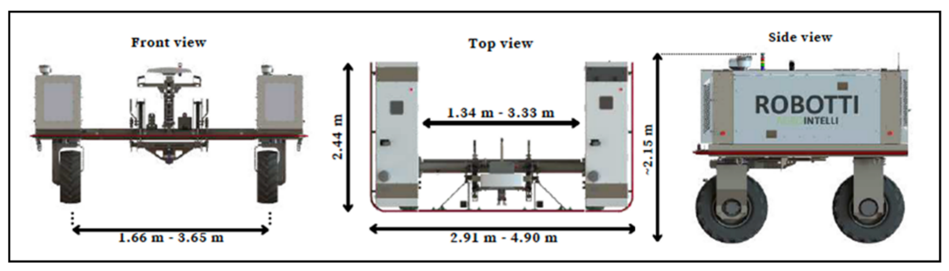
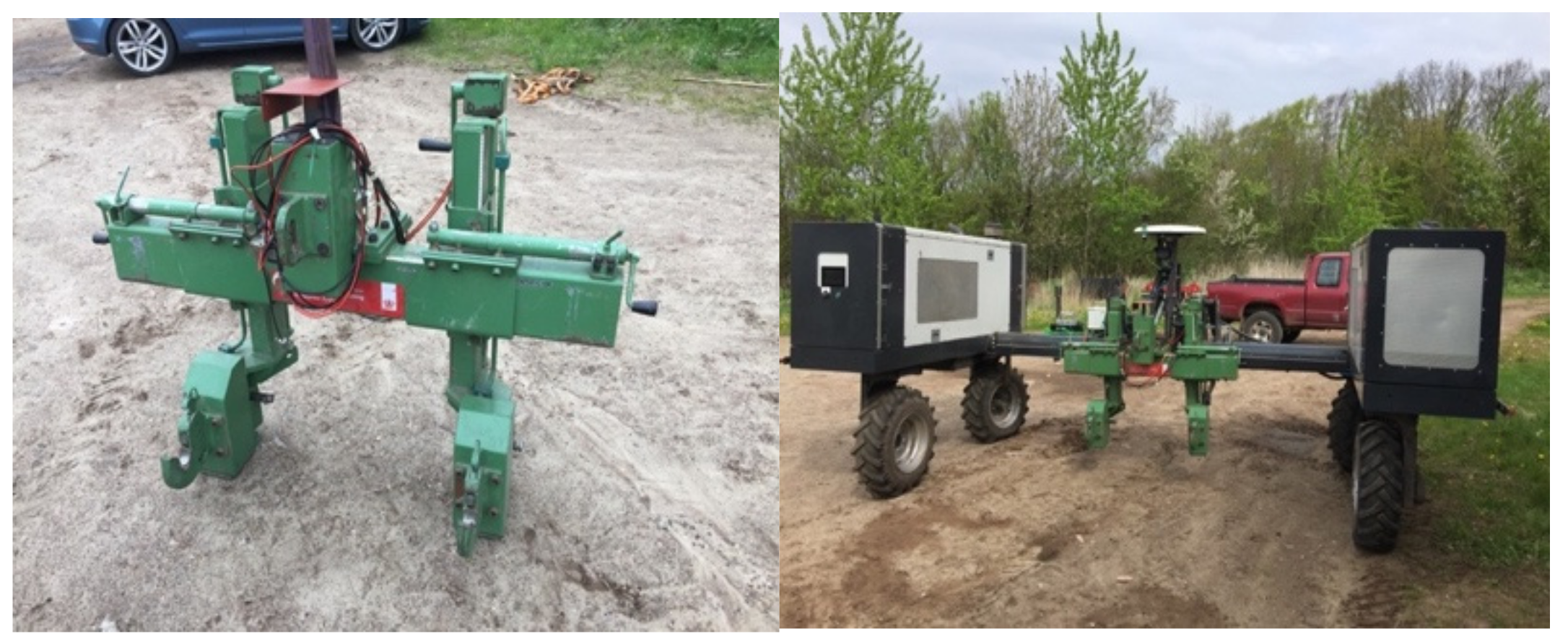
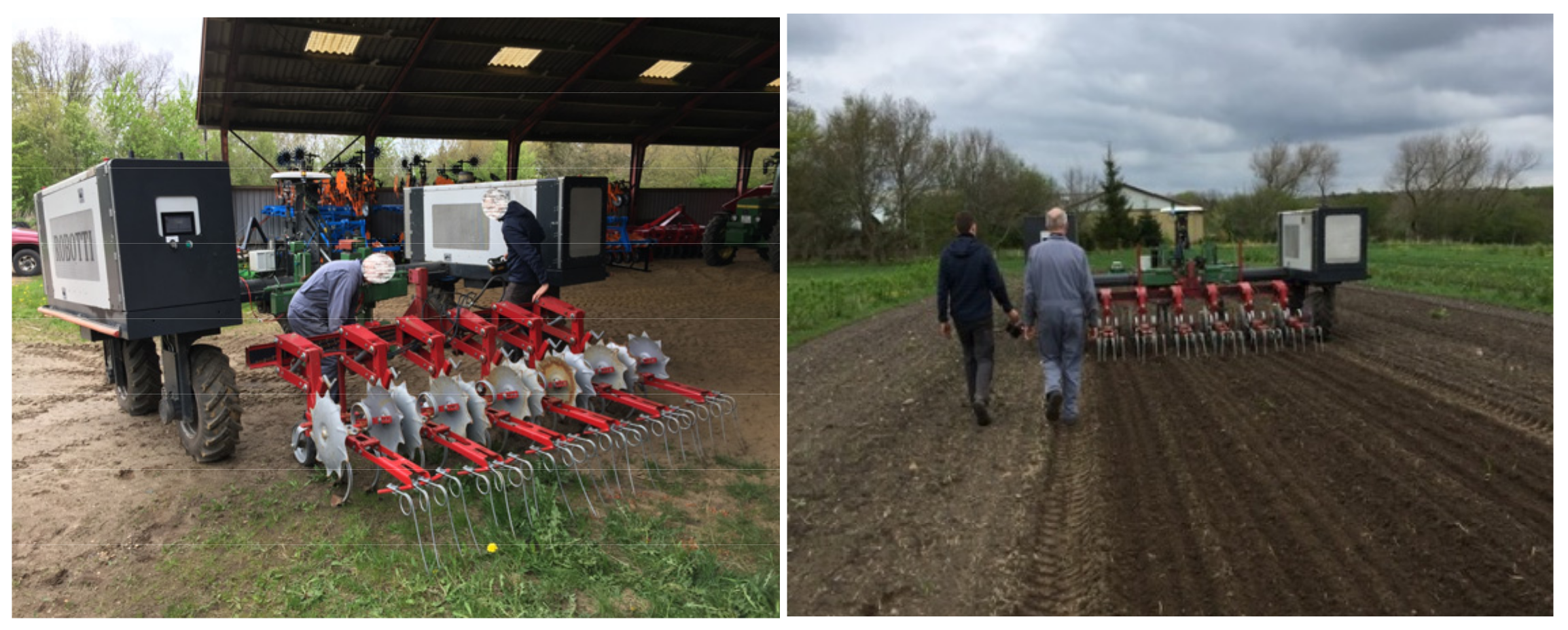
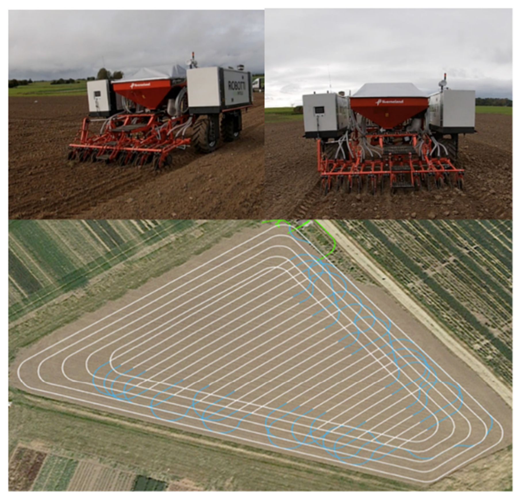
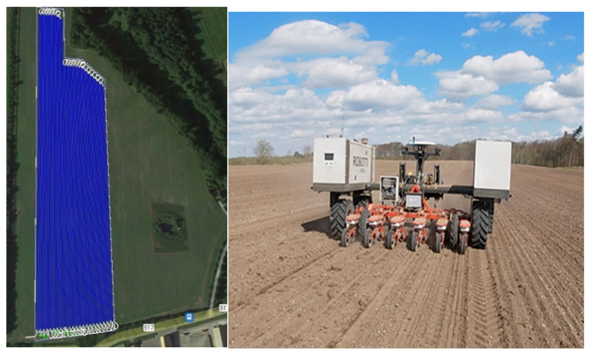
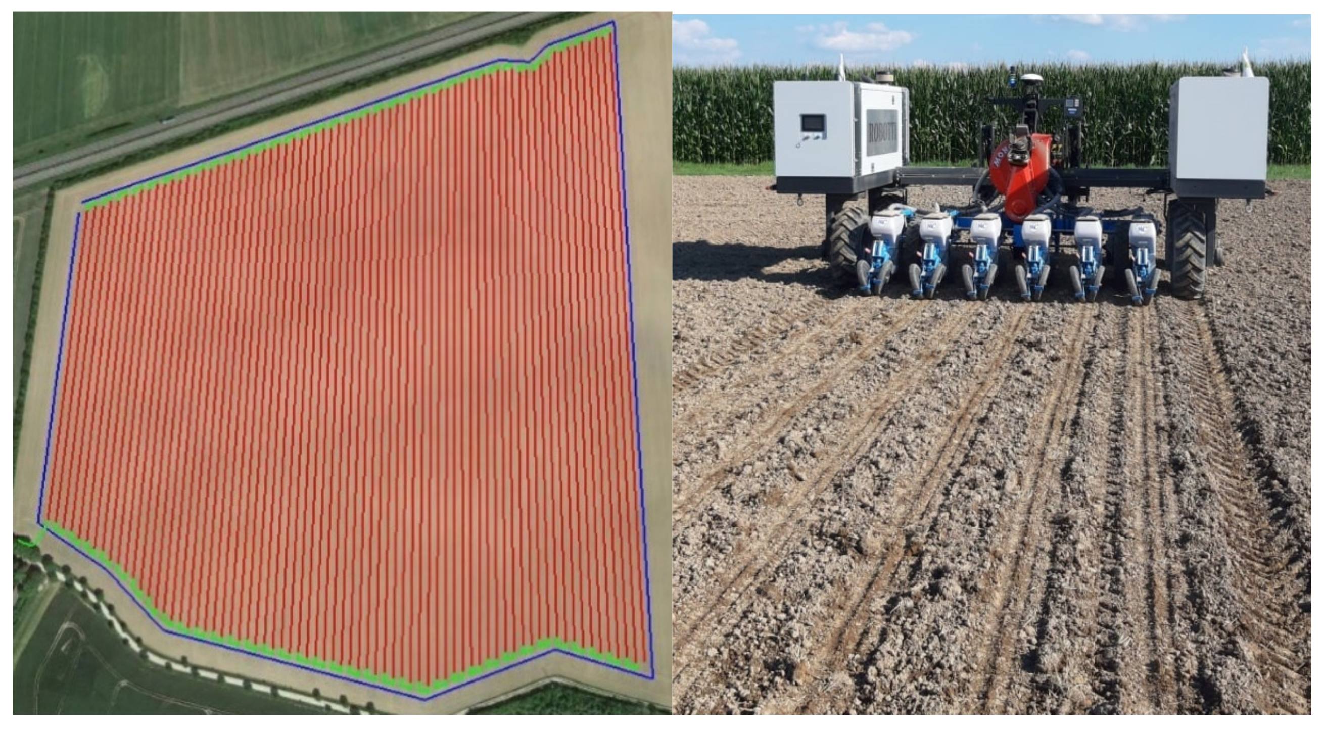
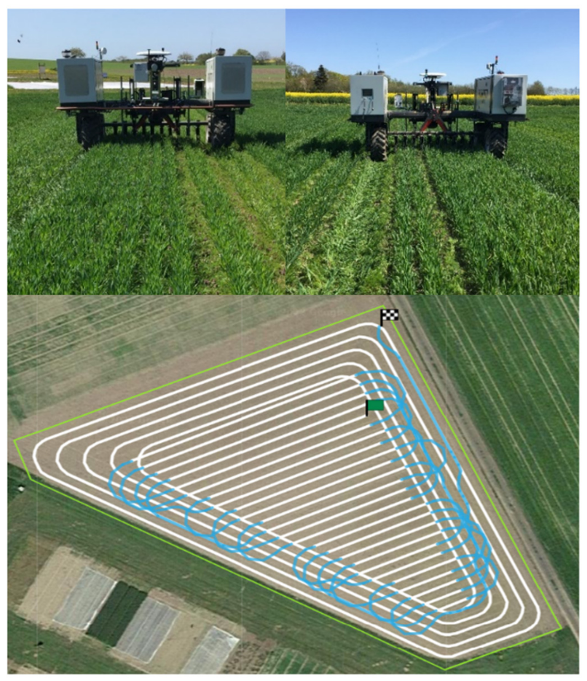
2.1. The Robot
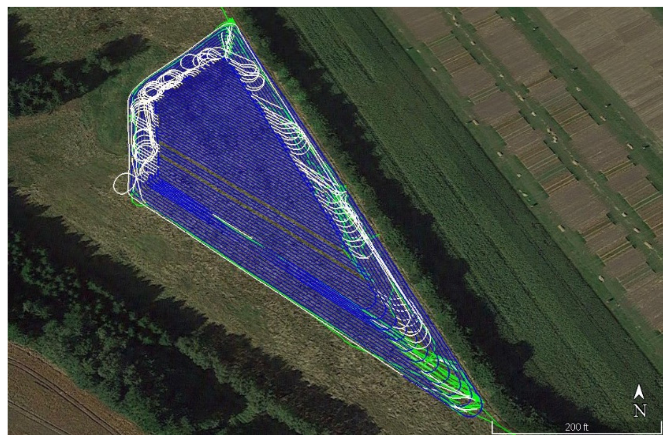
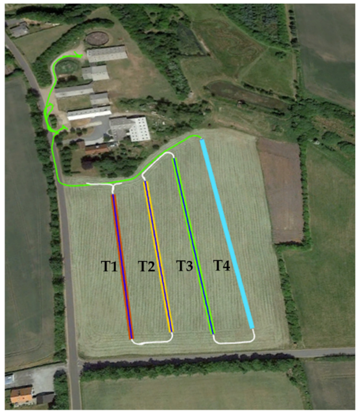
2.2. Monitoring, Measuring, and Analyzing of Robot’s In-Field Operations
2.3. Operational Factors
2.3.1. Field Efficiency
2.3.2. Effective Field Capacity
2.3.3. Theoretical Field Capacity
2.4. Economic Factors
2.4.1. Ownership Costs
2.4.2. Operational Costs
2.5. Environmental Factors (CO2 Emission)
2.6. Comparing the Performance Parameters of a Robotic System with Conventional Agricultural Machinery
2.6.1. Comparing the Draft Force Required to Pull an Implementation
2.6.2. Case Study Description
3. Results and Discussion
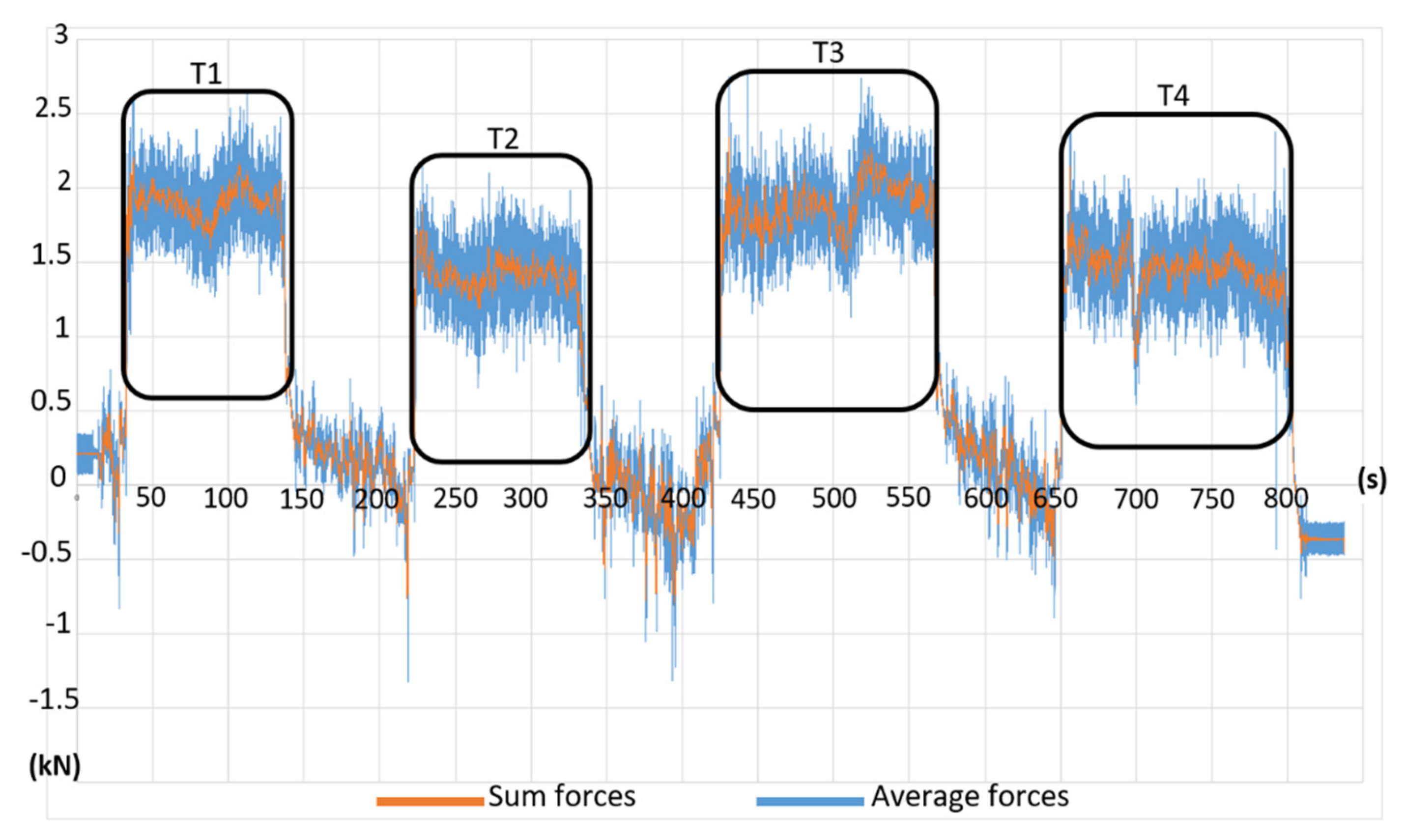
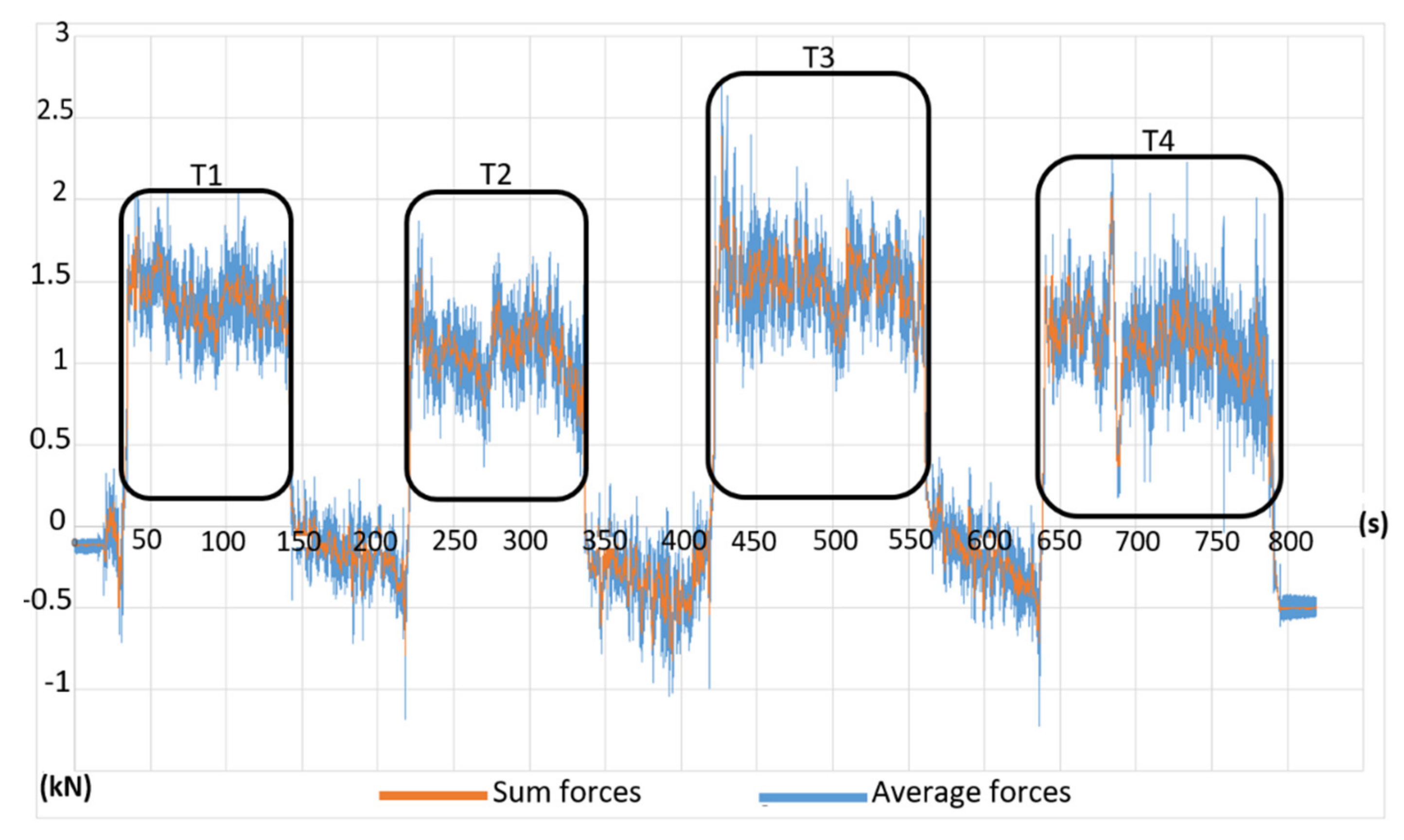
3.1. The Result of Draft Force Test
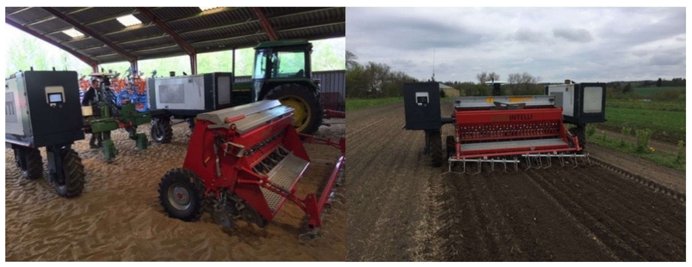
3.2. Seeding Operation
3.3. Weeding Operation
4. Conclusions
Author Contributions
Funding
Conflicts of Interest
References
- Moysiadis, V.; Tsolakis, N.; Katikaridis, D.; Sørensen, C.; Pearson, S.; Bochtis, D. Mobile robotics in agricultural operations: A narrative review on planning aspects. Appl. Sci. 2020, 10, 3453. [Google Scholar] [CrossRef]
- Marinoudi, V.; Sørensen, C.; Pearson, S.; Bochtis, D. Robotics and labour in agriculture. A context consideration. Biosyst. Eng. 2019, 184, 111–121. [Google Scholar] [CrossRef]
- Lampridi, M.; Kateris, D.; Vasileiadis, G.; Marinoudi, V.; Pearson, S.; Sørensen, C. A case-based economic assessment of robotics employment in precision arable farming. Agronomy 2019, 9, 175. [Google Scholar] [CrossRef]
- Saidani, M.; Pan, E.; Kim, H.; Greenlee, A.; Wattonville, J.; Yannou, B.; Leroy, Y.; Cluzel, F. Assessing the environmental and economic sustainability of autonomous systems: A case study in the agricultural industry. Procedia CIRP 2020, 90, 209–214, ISSN 2212-8271. [Google Scholar] [CrossRef]
- Duckett, T.; Pearson, S.; Blackmore, S.; Grieve, B. Agricultural Robotics: The Future of Robotic Agriculture. UK-RAS White Papers; UK-RAS: Leeds, UK, 2018; ISSN 2398-4414. [Google Scholar] [CrossRef]
- Goense, D. The economics of autonomous vehicles. In Proceedings of the VDI-MEG Conference on Agricultural Engineering, VDI-Tatung Landtechnic, Hannover, Germany, 7–8 November 2003. [Google Scholar]
- Have, H. Effects of automation on sizes and costs of tractor and machinery. In Proceedings of the European Society of Agricultural Engineers, Paper 285, Leuven, Belgium, 12–16 September 2004. [Google Scholar]
- Sørensen, C.G.; Madsen, N.A.; Jacobsen, B.H. Organic farming scenarios: Operational analysis and costs of implementing innovative technologies. Biosyst. Eng. 2005, 91, 127–137. [Google Scholar] [CrossRef]
- Pedersen, S.M.; Fountas, S.; Sørensen, C.G.; Van Evert, F.K.; Blackmore, B.S. Robotic seeding: Economic perspectives. In Precision Agriculture: Technology and Economic Perspectives. Progress in Precision Agriculture; Pedersen, S., Lind, K., Eds.; Springer: Cham, Switzerland, 2017. [Google Scholar] [CrossRef]
- Shaheb, M.R.; Venkatesh, R.; Shearer, S.A. A review on the effect of soil compaction and its management for sustainable crop production. J. Biosyst. Eng. 2021, 46, 417–439. [Google Scholar] [CrossRef]
- Pedersen, S.M.; Fountas, S.; Have, H.; Blackmore, B.S. Agricultural Robots—System Analysis and economic feasibility. Precis. Agric. 2006, 7, 295–308. [Google Scholar] [CrossRef]
- Robotic Solutions for Sustainable Farming. Available online: https://dahliarobotics.com (accessed on 23 January 2023).
- Powerful, Energy-Efficient and Autonomous. Available online: https://farming-revolution.com (accessed on 23 January 2023).
- Product. Available online: https://farmdroid.dk/en/product (accessed on 23 January 2023).
- Autonomous Oz Weeding Robot. Available online: https://www.naio-technologies.com/en/oz (accessed on 23 January 2023).
- Robotti 150D, Agrointelli. Available online: https://agrointelli.com/robotti/150D/ (accessed on 14 December 2022).
- Bhimanpallewar, R.; Narasingarao, M. AgriRobot: Implementation and evaluation of an automatic robot for seeding and fertilizer microdosing in precision agriculture. Int. J. Agric. Resour. Gov. Ecol. 2020, 16, 33. [Google Scholar] [CrossRef]
- Naik, N.S.; Shete, V.V.; Danve, S.R. Precision agriculture robot for seeding function. In Proceedings of the International Conference on Inventive Computation Technologies (ICICT), Coimbatore, India, 26–27 August 2016; p. 13. [Google Scholar] [CrossRef]
- Sunitha, K.A.; Suraj, G.S.G.S.; Sowrya, C.H.P.N.; Sriram, G.A.; Shreyas, D.; Srinivas, T. Agricultural robot designed for seeding mechanism. In IOP Conference Series: Materials Science and Engineering; IOP Publishing: Bristol, UK, 2017; Volume 197. [Google Scholar]
- Gonzalez-de-Soto, M.; Emmi, L.; Perez-Ruiz, M.; Aguera, J.; Gonzalez-de-Santos, P. Autonomous systems for precise spraying: Evaluation of a robotized patch sprayer. Biosyst. Eng. 2016, 146, 165–182. [Google Scholar] [CrossRef]
- Berenstein, R.; Edan, Y. Human-robot collaborative site-specific sprayer. J. Field Robot. 2017, 34, 1519–1530. [Google Scholar] [CrossRef]
- Oduma, O.; Oluka, S.; Nwakuba, N.; Ntunde, D. Agricultural field machinery selection and utilization for improved farm operations in South-East Nigeria: A review. Poljopr. Teh. 2019, 44, 44–58. [Google Scholar] [CrossRef]
- Pflueger, B. How to Calculate Machinery Ownership and Operating Costs. SDSU Extension Circulars 2015. Paper 485. Available online: http://openprairie.sdstate.edu/extension_circ/485 (accessed on 30 January 2023).
- Edwards, W. Estimating Farm Machinery Costs: Ag Decision Maker, Lowa State University Extension and Outreach. Available online: https://www.extension.iastate.edu/agdm/crops/html/a3-29.html (accessed on 31 October 2022).
- American Society of Agricultural and Biological Engineers (ASABE). Agricultural Machinery Management—ASAE EP496.3 FEB2006 (R2015); ASABE: St. Joseph, MI, USA, 2006. [Google Scholar]
- Tihanov, G.; Ivanov, N. Fuel consumption of a machine-tractor unit in direct sowing of wheat. Agric. Sci. Technol. 2021, 13, 40–42. [Google Scholar] [CrossRef]
- Hunt, D.; Wilson, D. Farm Power and Machinery Management, 11th ed.; Waveland Press: Long Grove, IL, USA, 2015; (ED-TECH). [Google Scholar]
- NTTL. Nebraska Tractor Test 2085 for John Deere 7250R.Lincoln, NE: Nebraska Tractor Test Laboratory 2014. Available online: http://tractortestlab.unl.edu (accessed on 30 January 2023).
- ANSI ASABE D497-4-2003 Scribd. Available online: https://www.scribd.com/document/345945527/ANSI-ASABE-D497-4-2003 (accessed on 1 November 2022).
- Manzone, M.; Calvo, A. Energy and CO2 analysis of poplar and maize crops for biomass production in north Italy. Renew Energy 2016, 86, 675–681. [Google Scholar] [CrossRef]
- Soane, B.D.; Ball, B.C.; Arvidsson, J.; Basch, G.; Moreno, F.; Roger-Estrade, J. No-till in northern, western and south-western Europe: A review of problems and opportunities for crop production and the environment. Soil Tillage Res. 2012, 118, 66–87. [Google Scholar] [CrossRef]
- Filipovic, D.; Kosutic, S.; Gospodaric, Z.; Zimmer, R.; Banaj, D. The possibilities of fuel savings and the reduction of CO2 emissions in the soil tillage in Croatia. Agric. Ecosyst. Environ. 2006, 115, 290–294. [Google Scholar] [CrossRef]
- American Society of Agricultural and Biological Engineers (ASABE). Agricultural Machinery Management Data—ASAE D497.5 FEB2006; ASABE: St. Joseph, MI, USA, 2006. [Google Scholar]
- Augustin, K.; Kuhwald, M.; Brunotte, J.; Duttmann, R. Wheel load and wheel pass frequency as indicators for soil compaction risk: A four-year analysis of traffic intensity at Field Scale. Geosciences 2020, 10, 292. [Google Scholar] [CrossRef]
- Pulido-Moncada, M.; Munkholm, L.J.; Schjønning, P. Wheel load, repeated wheeling, and traction effects on subsoil compaction in Northern Europe. Soil Tillage Res. 2019, 186, 300–309. [Google Scholar] [CrossRef]
- Redhead, F.; Snow, S.; Vyas, D.; Bawden, O.; Russell, R.; Perez, T.; Brereton, M. Bringing the Farmer Perspective to Agricultural Robots. In Proceedings of the 33rd Annual ACM Conference Extended Abstracts on Human Factors in Computing Systems 2015, Seoul, Republic of Korea, 18–23 April 2015; ACM: New York, NY, USA, 2015; pp. 1067–1072. [Google Scholar] [CrossRef]
- Rotz, S.; Gravely, E.; Mosby, I.; Duncan, E.; Finnis, E.; Horgan, M.; LeBlanc, J.; Martin, R.; Neufeld, H.T.; Nixon, A.; et al. Automated pastures and the digital divide: How agricultural technologies are shaping labour and rural communities. J. Rural. Stud. 2019, 68, 112–122. [Google Scholar] [CrossRef]
- Spykman, O.; Gabriel, A.; Ptacek, M.; Gandorfer, M. Farmers’ perspectives on field crop robots—Evidence from Bavaria, Germany. Comput. Electron. Agric. 2021, 186, 106176. [Google Scholar] [CrossRef]


| Machine | Field Efficiency | Field Speed | Estimated Life | Total Life R&M Cost | Repair Factors | |||
|---|---|---|---|---|---|---|---|---|
| Range % | Typical % | Range (km/h) | Typical (km/h) | H | % of List Price | RF1 | RF2 | |
| Grain drill | 55–80 | 70 | 6.5–11.0 | 8.0 | 1500 | 75 | 0.32 | 2.1 |
| Tractors (4-wheel drive & crawler) | 16,000 | 80 | 0.003 | 2.0 | ||||
| Average Fuel Consumption (John Deere 7250 R) | |||
|---|---|---|---|
| Working width sowing machine (m) | 3 | 4 | 6 |
| Power demand (kW) | 90 | 105 | 155 |
| Mode | Consumption (L/h) | ||
| Working mode (sowing) | 13.82 | 15.64 | 23.08 |
| Transportation mode | 9.61 | 11.21 | 16.55 |
| Static mode | 4.30 | 4.30 | 4.30 |
| Implement | Width | Machine Parameters | Soil Parameters | Range ±% | ||||
|---|---|---|---|---|---|---|---|---|
| A | B | C | F1 | F2 | F3 | |||
| Major Tillage Tools | ||||||||
| Rod Weeder | m | 210 | 10.7 | 0.0 | 1.0 | 0.85 | 0.65 | 25 |
| Minor Tillage Tools | ||||||||
| Grain Drill | rows | 720 | 0.0 | 0.0 | 1.0 | 0.92 | 0.79 | 35 |
| Robot-Working Width 3 [m] | Tractor-Working Width 3 [m] | Tractor-Working Width 4 [m] | Tractor-Working Width 6 [m] | ||
|---|---|---|---|---|---|
| Ownership costs parameters | Purchase price (EUR) | 144,500 | 269,200 | 273,200 | 280,700 |
| Salvage value (EUR) | 14,450 | 26,920 | 27,320 | 28,070 | |
| Economical life (years) | 10 | 15 | 15 | 15 | |
| Average interest rate (%) | 9 | 9 | 9 | 9 | |
| Depreciation (EUR/year) | 13,005 | 16,152 | 16,392 | 16,842 | |
| Interest (EUR/year) | 5852 | 10,903 | 11,065 | 11,368 | |
| Insurance and Taxes (EUR/year) | 1445 | 2692 | 2732 | 2807 | |
| Housing (EUR/year) | 1445 | 2692 | 2732 | 2807 | |
| Ownership costs (EUR/year) | 21,747 | 32,439 | 32,921 | 33,824 | |
| Economical life (h) | 6000 | 16,000 | 16,000 | 16,000 | |
| Ownership costs (EUR/h) | 3.62 | 2.03 | 2.06 | 2.11 | |
| Robot-Working Width 2.4 [m] | Tractor-Working Width 2.4 [m] | Tractor-Working Width 4 [m] | Tractor-Working Width 6 [m] | ||
|---|---|---|---|---|---|
| Ownership costs parameters | Purchase price (EUR) | 144,200 | 268,900 | 275,700 | 284,600 |
| Salvage value (EUR) | 14,420 | 26,890 | 27,570 | 28,460 | |
| Economical life (years) | 10 | 15 | 15 | 15 | |
| Average interest rate (%) | 9 | 9 | 9 | 9 | |
| Depreciation (EUR/year) | 12,978 | 16,134 | 16,542 | 17,076 | |
| Interest (EUR/year) | 5840 | 10,890 | 11,166 | 11,526 | |
| Insurance & Taxes (EUR/year) | 1442 | 2689 | 2757 | 2846 | |
| Housing (EUR/year) | 1442 | 2689 | 2757 | 2846 | |
| Ownership costs (EUR/year) | 21,702 | 32,402 | 33,222 | 34,294 | |
| Economical life (h) | 6000 | 16,000 | 16,000 | 16,000 | |
| Ownership costs (EUR/h) | 3.62 | 2.03 | 2.08 | 2.14 | |
| Calculation of Required Energy for Pulling the Seeder | |||||
|---|---|---|---|---|---|
| Seeding/T1 | Seeding/T2 | Seeding/T3 | Seeding/T4 | Average | |
| The average horizontal force (kN) | 1.85 | 1.39 | 1.87 | 1.44 | 1.64 |
| Travel time (s) | 109 | 114 | 143 | 150 | 129 |
| Traveled distance (track length) (m) | 131 | 141 | 170 | 189 | 157.75 |
| kW h | 0.067 | 0.055 | 0.088 | 0.076 | 0.072 |
| kW h/ha | 1.70 | 1.30 | 1.73 | 1.33 | 1.52 |
| Calculation of Required Energy for Pulling the Weeder | |||||
|---|---|---|---|---|---|
| Weeder/T1 | Weeder/T2 | Weeder/T3 | Weeder/T4 | Average | |
| The average horizontal force (kN) | 1.38 | 1.07 | 1.50 | 1.12 | 1.27 |
| Travel time (s) | 106 | 115 | 139 | 148 | 127 |
| Traveled distance (track length) (m) | 131 | 141 | 170 | 189 | 157.75 |
| kW h | 0.050 | 0.042 | 0.071 | 0.059 | 0.056 |
| kW h/ha | 1.28 | 0.99 | 1.39 | 1.04 | 1.18 |
| Robot-Working Width 3 [m] | Tractor-Working Width 3 [m] | Tractor-Working Width 4 [m] | Tractor-Working Width 6 [m] | |
|---|---|---|---|---|
| Field working time [min] | 36 | 15.4 | 11.8 | 8 |
| Non-working time [min] | 31 | 13.7 | 10.6 | 7.12 |
| Static time [min] | 0 | 0.95 | 0.34 | 0.34 |
| Total time [min] | 67 | 30.05 | 22.74 | 15.46 |
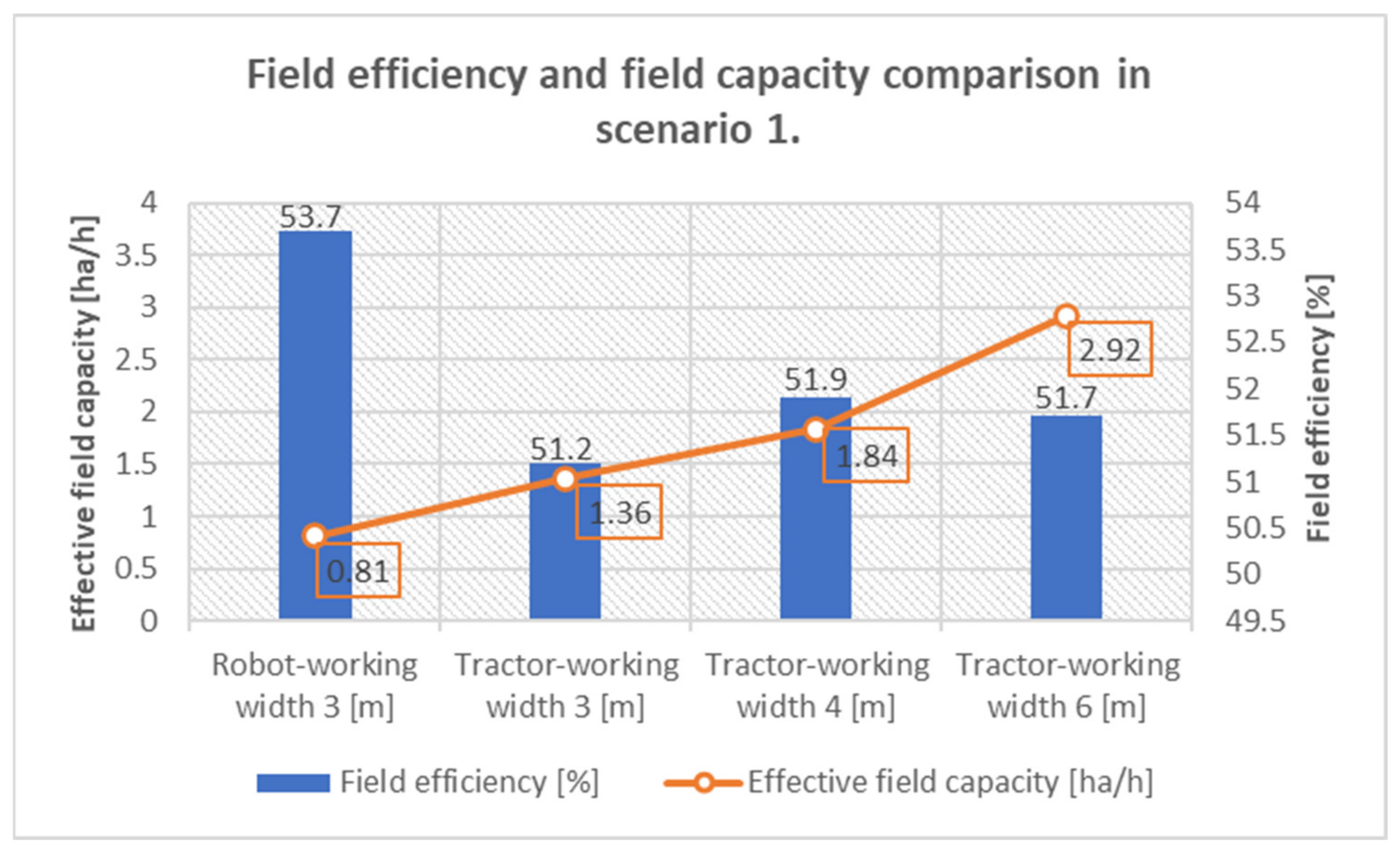
| Field efficiency [%] | 53.7 | 51.2 | 51.9 | 51.7 |
| Effective field capacity [ha/h] | 0.81 | 1.36 | 1.84 | 2.92 |
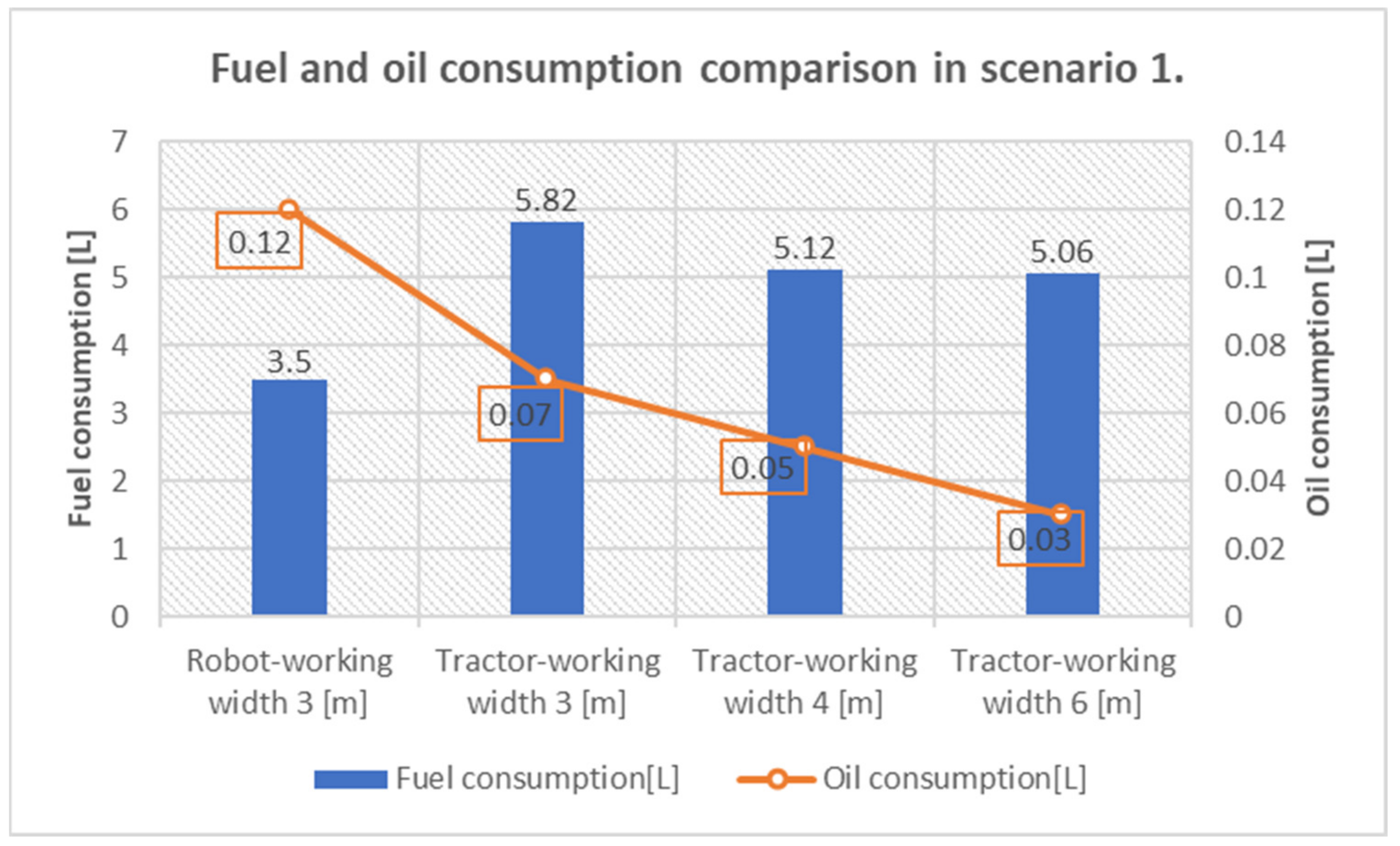
| Fuel consumption [L] | 3.5 | 5.82 | 5.12 | 5.06 |
| Oil consumption [L] | 0.12 | 0.07 | 0.05 | 0.03 |
| Energy cost [EUR] | 7 | 11.64 | 10.24 | 10.12 |
| Lubrication cost [EUR] | 0.04 | 0.02 | 0.015 | 0.01 |
| Labour cost [EUR] | 16.53 | 14.82 | 11.22 | 7.63 |
| Repair and Maintenance [EUR] | 13.1 | 6.76 | 5.2 | 3.62 |
| Operational costs [EUR] | 36.67 | 33.24 | 26.68 | 21.38 |
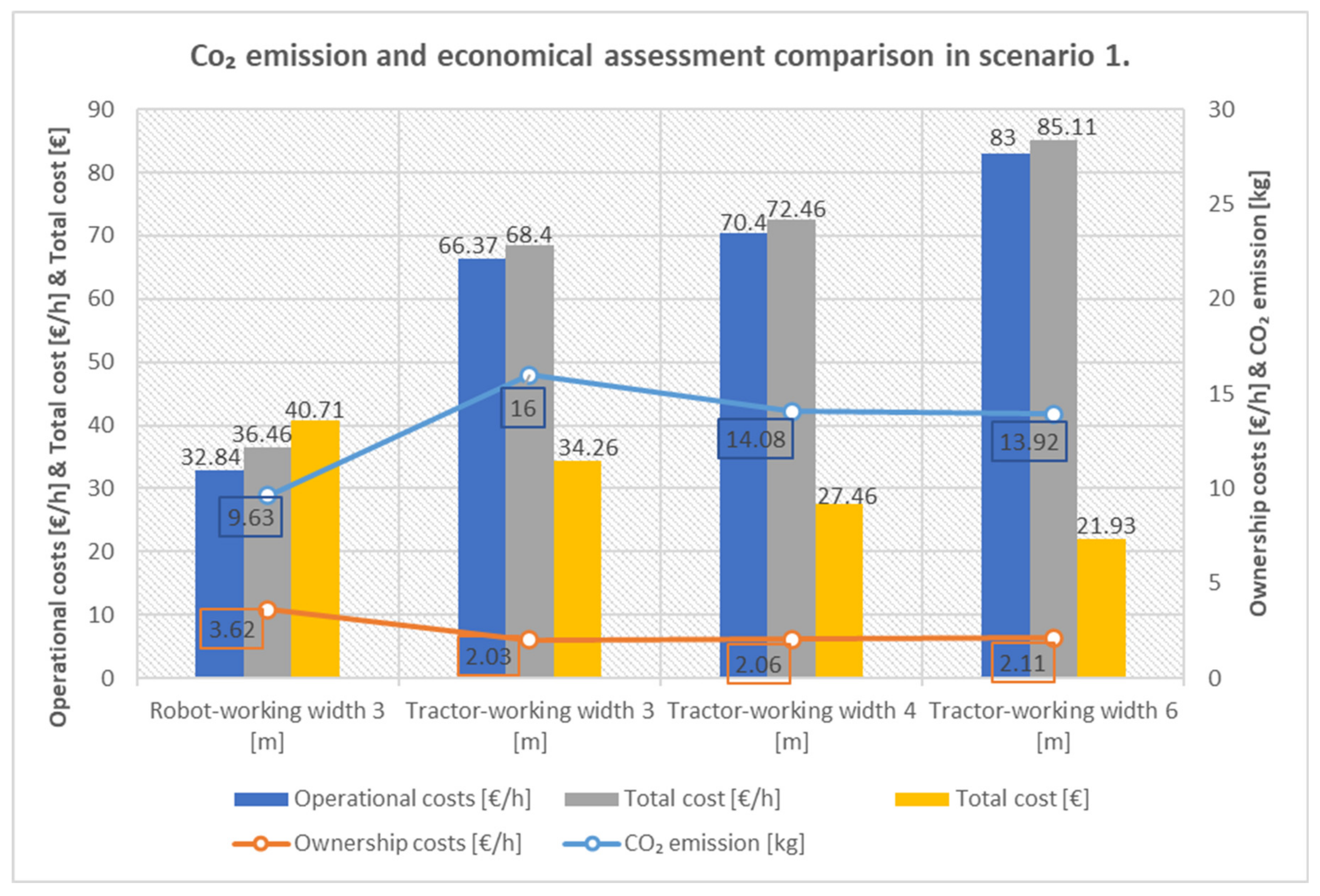
| Operational costs [EUR/h] | 32.84 | 66.37 | 70.4 | 83 |
| Ownership costs [EUR/h] | 3.62 | 2.03 | 2.06 | 2.11 |
| Total cost per hour [EUR/h] | 36.46 | 68.4 | 72.46 | 85.11 |
| Total cost [EUR] | 40.71 | 34.26 | 27.46 | 21.93 |
| CO2 emission [kg] | 9.63 | 16 | 14.08 | 13.92 |
| Robot-Working Width 3 [m] | Tractor-Working Width 3 [m] | Tractor-Working Width 4 [m] | Tractor-Working Width 6 [m] | |
|---|---|---|---|---|
| Field working time [min] | 167 | 167.2 | 126.1 | 83.6 |
| Non-working time [min] | 70 | 80.3 | 68.9 | 43.9 |
| Static time [min] | 9 | 12.75 | 4.5 | 4.5 |
| Total time [min] | 246 | 260.25 | 199.5 | 132 |
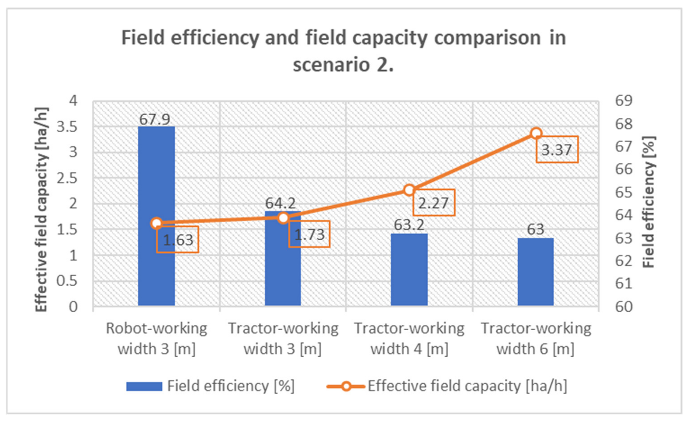
| Field efficiency [%] | 67.9 | 64.2 | 63.2 | 63 |
| Effective field capacity [ha/h] | 1.63 | 1.73 | 2.27 | 3.37 |
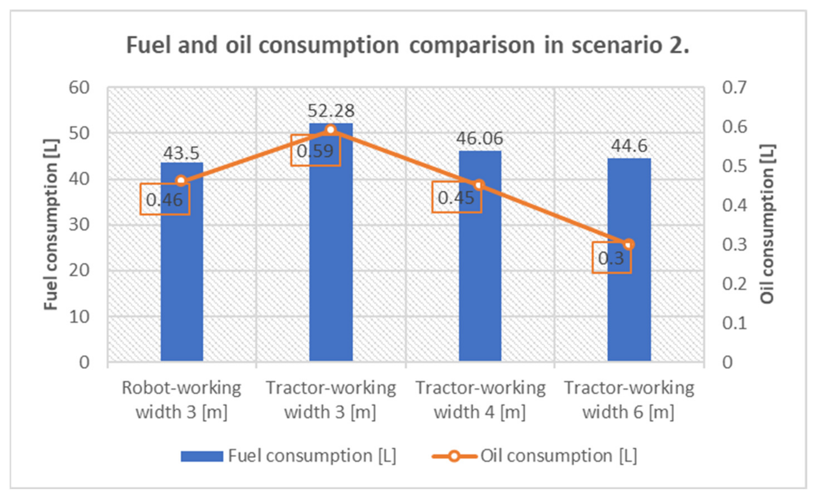
| Fuel consumption [L] | 43.5 | 52.28 | 46.06 | 44.6 |
| Oil consumption [L] | 0.46 | 0.59 | 0.45 | 0.3 |
| Energy cost [EUR] | 87 | 104.56 | 92.12 | 89.2 |
| Lubrication cost [EUR] | 0.138 | 0.177 | 0.135 | 0.09 |
| Labour cost [EUR] | 60.68 | 128.4 | 98.42 | 65.12 |
| Repair and Maintenance [EUR] | 47.97 | 58.56 | 45.55 | 30.89 |
| Operational costs [EUR] | 195.79 | 291.7 | 236.23 | 185.3 |
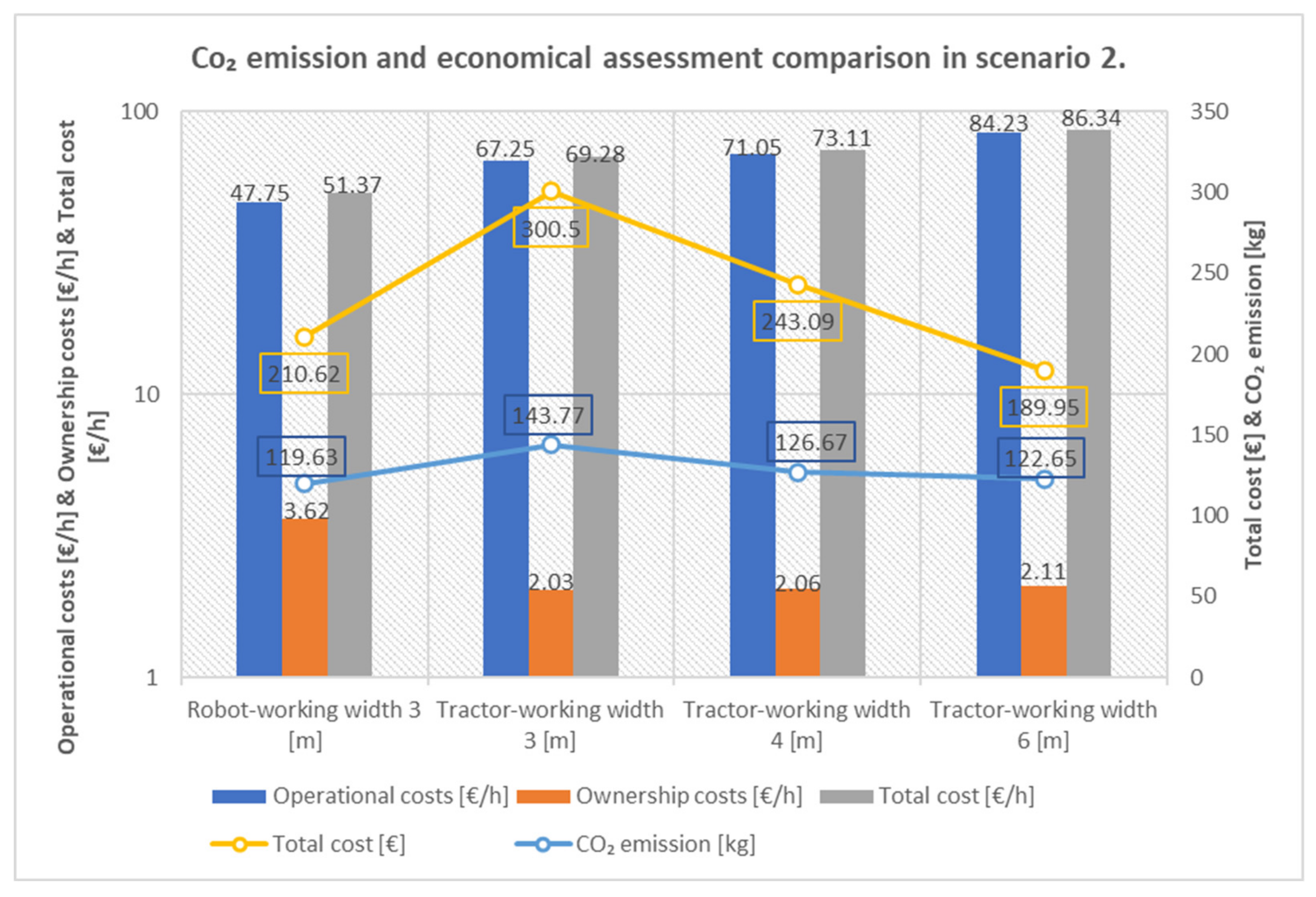
| Operational costs [EUR/h] | 47.75 | 67.25 | 71.05 | 84.23 |
| Ownership costs [EUR/h] | 3.62 | 2.03 | 2.06 | 2.11 |
| Total cost per hour [EUR/h] | 51.37 | 69.28 | 73.11 | 86.34 |
| Total cost [EUR] | 210.62 | 300.5 | 243.09 | 189.95 |
| CO2 emission [kg] | 119.63 | 143.77 | 126.67 | 122.65 |
| Robot-Working Width 3 [m] | Tractor-Working Width 3 [m] | Tractor-Working Width 4 [m] | Tractor-Working Width 6 [m] | |
|---|---|---|---|---|
| Field working time [min] | 514.1 | 479.5 | 399.3 | 267.4 |
| Non-working time [min] | 89.7 | 117.4 | 101 | 69 |
| Static time [min] | 118.2 | 96.1 | 70.4 | 42 |
| Total time [min] | 722 | 693 | 571 | 378 |
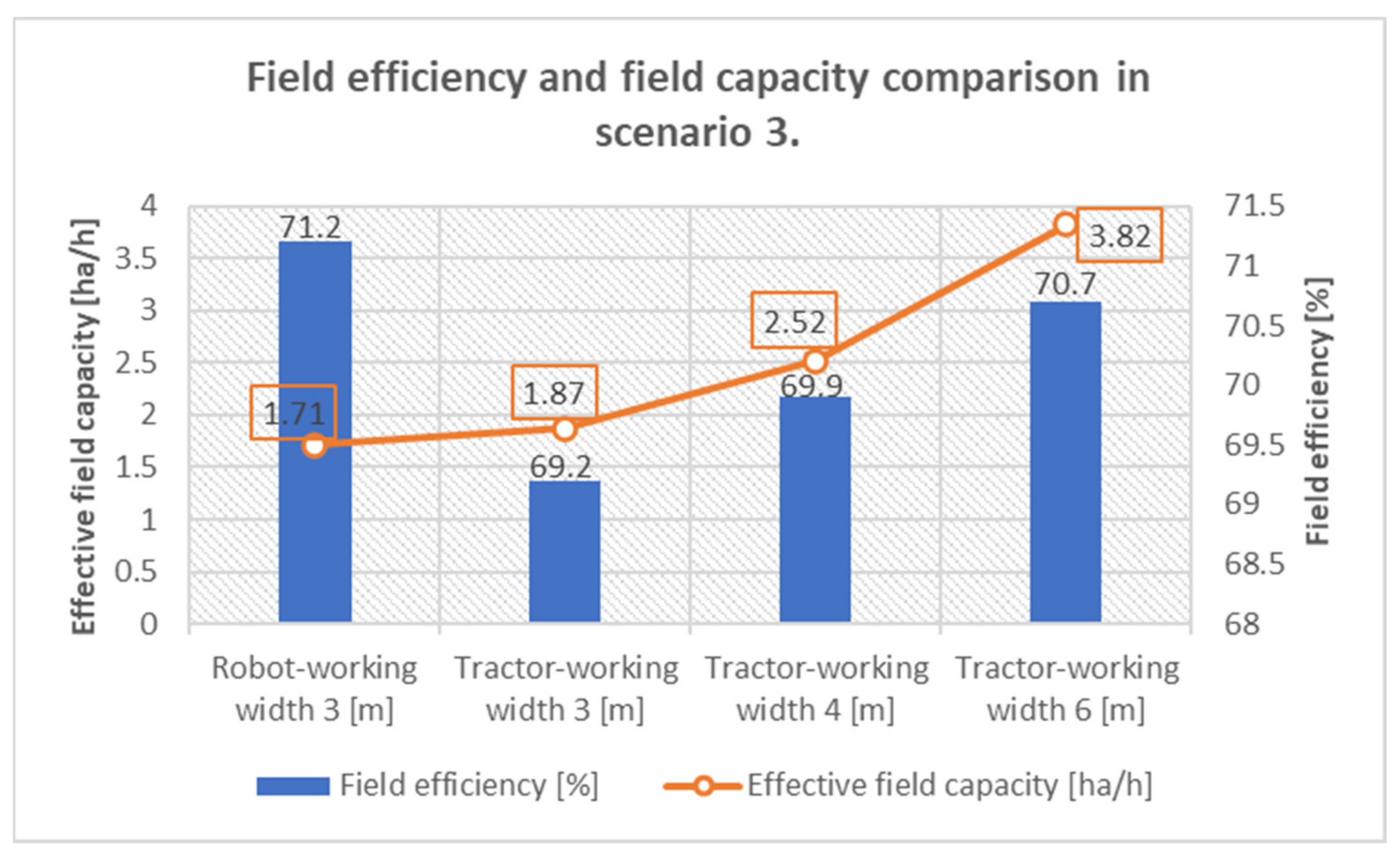
| Field efficiency [%] | 71.2 | 69.2 | 69.9 | 70.7 |
| Effective field capacity [ha/h] | 1.71 | 1.87 | 2.52 | 3.82 |
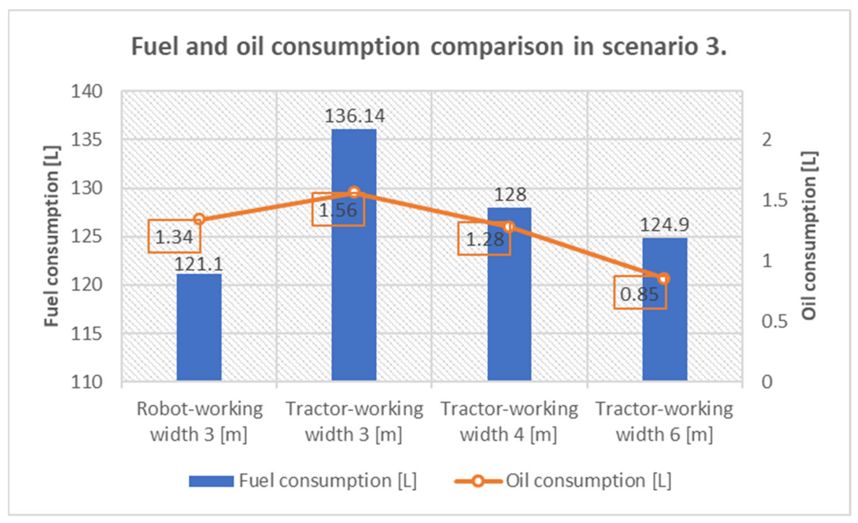
| Fuel consumption [L] | 121.1 | 136.14 | 128 | 124.9 |
| Oil consumption [L] | 1.34 | 1.56 | 1.28 | 0.85 |
| Energy cost [EUR] | 242.2 | 272.28 | 256 | 249.8 |
| Lubrication cost [EUR] | 0.4 | 0.47 | 0.38 | 0.255 |
| Labour cost [EUR] | 178.1 | 341.9 | 281.7 | 186.48 |
| Repair and Maintenance [EUR] | 140.79 | 155.93 | 130.38 | 88.45 |
| Operational costs [EUR] | 561.5 | 770.6 | 668.5 | 525 |
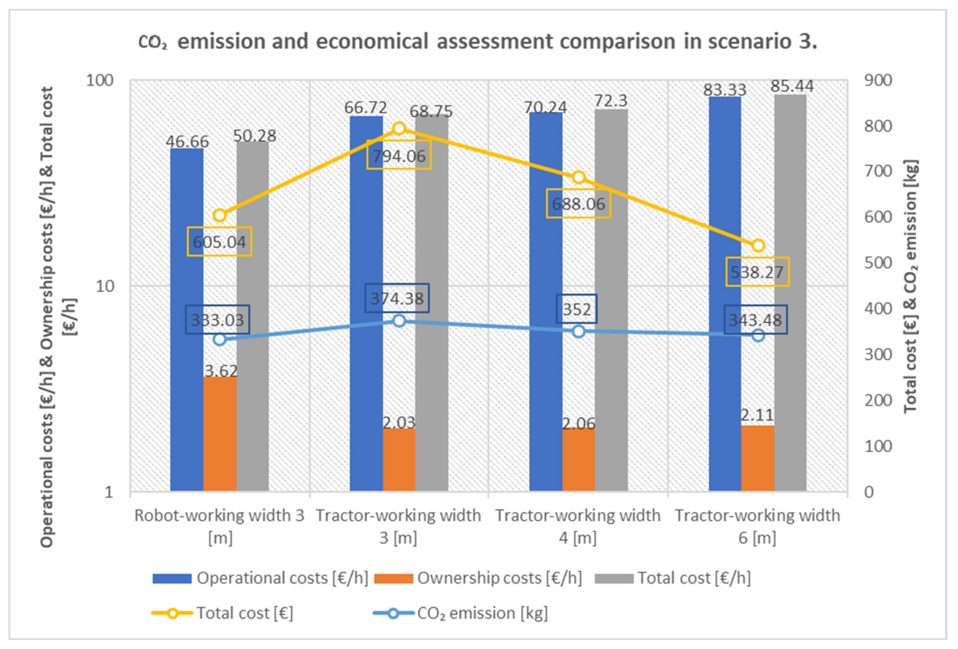
| Operational costs [EUR/h] | 46.66 | 66.72 | 70.24 | 83.33 |
| Ownership costs [EUR/h] | 3.62 | 2.03 | 2.06 | 2.11 |
| Total cost per hour [EUR/h] | 50.28 | 68.75 | 72.3 | 85.44 |
| Total cost [EUR] | 605.04 | 794.06 | 688.06 | 538.27 |
| CO2 emission [kg] | 333.03 | 374.38 | 352 | 343.48 |
| Robot-Working Width 2.4 [m] | Tractor-Working Width 2.4 [m] | Tractor-Working Width 4 [m] | Tractor-Working Width 6 [m] | |
|---|---|---|---|---|
| Field working time [min] | 43.23 | 26.5 | 14.8 | 9.98 |
| Non-working time [min] | 31.32 | 14.3 | 9.2 | 4.6 |
| Static time [min] | 1 | 6 | 4.65 | 4.65 |
| Total time [min] | 75.55 | 46.8 | 28.65 | 19.23 |
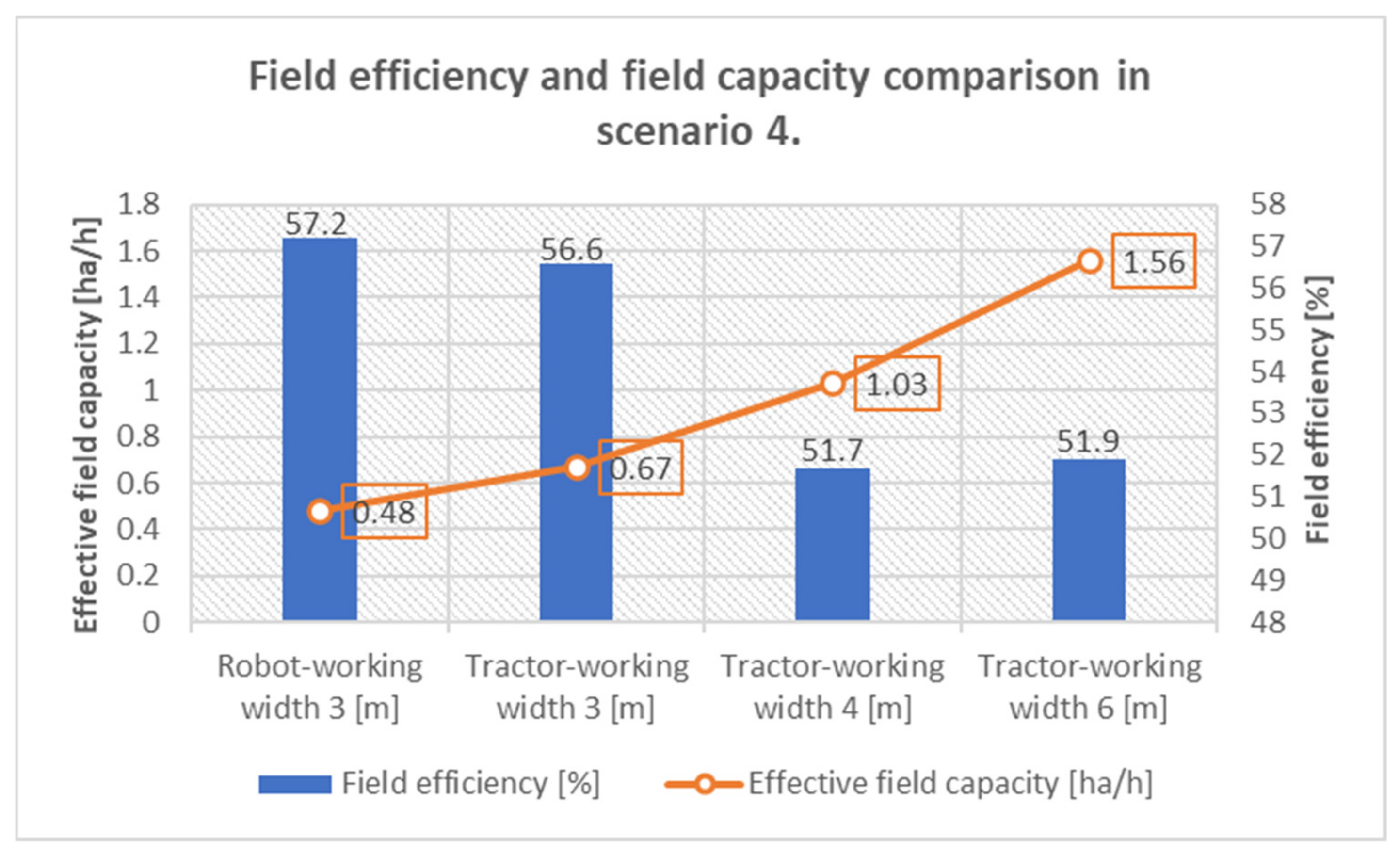
| Field efficiency [%] | 57.2 | 56.6 | 51.7 | 51.9 |
| Effective field capacity [ha/h] | 0.48 | 0.67 | 1.03 | 1.56 |
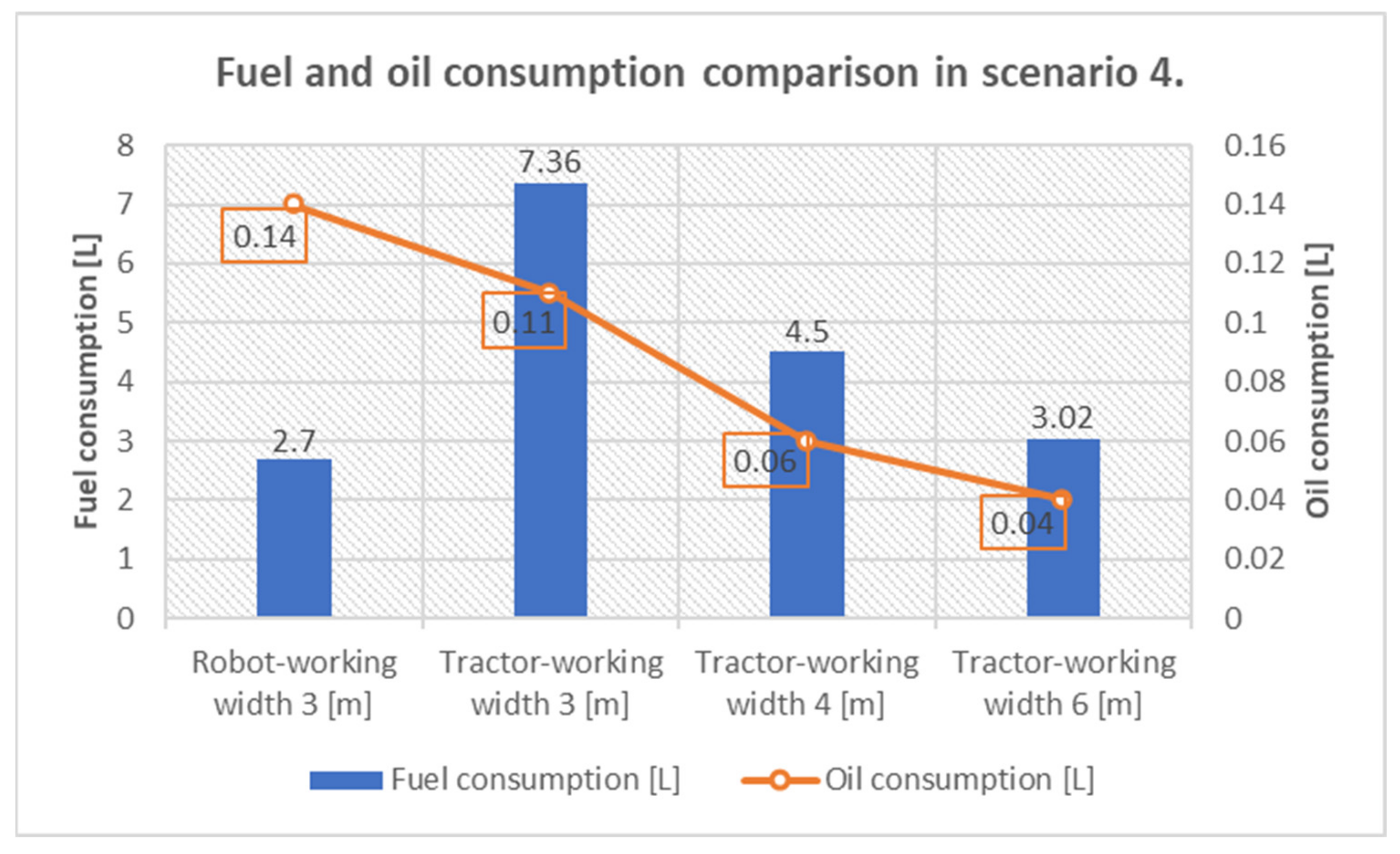
| Fuel consumption [L] | 2.7 | 7.36 | 4.5 | 3.02 |
| Oil consumption [L] | 0.14 | 0.11 | 0.06 | 0.04 |
| Energy cost [EUR] | 5.4 | 14.72 | 9 | 6.04 |
| Lubrication cost [EUR] | 0.04 | 0.03 | 0.02 | 0.01 |
| Labour cost [EUR] | 18.64 | 23.1 | 14.13 | 9.5 |
| Repair and Maintenance [EUR] | 14.73 | 10.5 | 6.6 | 4.6 |
| Operational costs [EUR] | 38.81 | 48.35 | 29.75 | 20.15 |
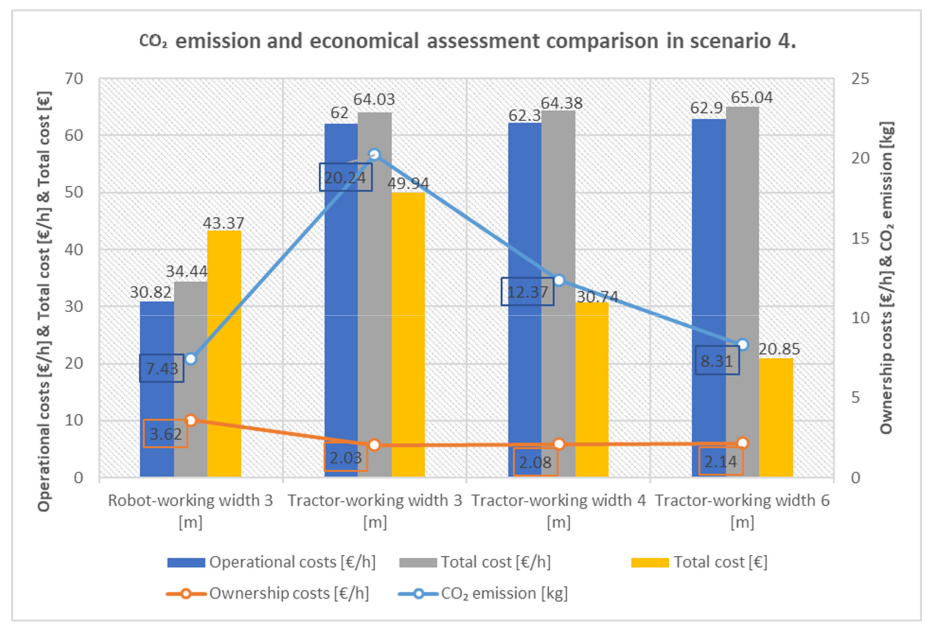
| Operational costs [EUR/h] | 30.82 | 62 | 62.3 | 62.9 |
| Ownership costs [EUR/h] | 3.62 | 2.03 | 2.08 | 2.14 |
| Total cost per hour [EUR/h] | 34.44 | 64.03 | 64.38 | 65.04 |
| Total cost [EUR] | 43.37 | 49.94 | 30.74 | 20.85 |
| CO2 emission [kg] | 7.43 | 20.24 | 12.37 | 8.31 |
| Robot-Working Width 3 [m] | Tractor-Working Width 3 [m] | Tractor-Working Width 4 [m] | Tractor-Working Width 6 [m] | |
|---|---|---|---|---|
| Field working time [min] | 514.1 | 479.5 | 399.3 | 267.4 |
| Non-working time [min] | 89.7 | 117.4 | 101 | 69 |
| Static time [min] | 118.2 | 96.1 | 70.4 | 42 |
| Idle time [min] | - | 40 | 40 | 40 |
| Total time [min] | 722 | 733 | 611 | 418 |
| Field efficiency [%] | 71.2 | 65.4 | 65.3 | 64 |
| Effective field capacity [ha/h] | 1.71 | 1.77 | 2.35 | 3.46 |
| Fuel consumption [L] | 121.1 | 136.14 | 128 | 124.9 |
| Oil consumption [L] | 1.34 | 1.56 | 1.28 | 0.85 |
| Energy cost [EUR] | 242.2 | 272.28 | 256 | 249.8 |
| Lubrication cost [EUR] | 0.4 | 0.47 | 0.38 | 0.255 |
| Labour cost [EUR] | 178.1 | 349.4 | 291.2 | 199.25 |
| Repair and Maintenance EUR] | 140.79 | 164.93 | 139.5 | 97.8 |
| Operational costs [EUR] | 561.5 | 787.1 | 687.1 | 547.11 |
| Operational costs [EUR/h] | 46.66 | 64.43 | 67.47 | 78.53 |
| Ownership costs [EUR/h] | 3.62 | 2.03 | 2.06 | 2.11 |
| Total cost per hour [EUR/h] | 50.28 | 66.46 | 69.53 | 80.64 |
| Total cost [EUR] | 604.2 | 811.92 | 708.05 | 561.8 |
| CO2 emission [kg] | 333.03 | 374.38 | 352 | 343.48 |
| Seeding Operation | ||||
|---|---|---|---|---|
| Tractor (3 m) | Tractor (4 m) | Tractor (6 m) | ||
| Ownership costs parameters | Purchase price (EUR) | 114,500 | 118,500 | 126,000 |
| Salvage value (EUR) | 11,450 | 11,850 | 12,600 | |
| Economical life (years) | 15 | 15 | 15 | |
| Average interest rate (%) | 9 | 9 | 9 | |
| Depreciation (EUR/year) | 6870 | 7110 | 7560 | |
| Interest (EUR/year) | 4637 | 4799 | 5103 | |
| Insurance & Taxes (EUR/year) | 1145 | 1185 | 1260 | |
| Housing (EUR/year) | 1145 | 1185 | 1260 | |
| Ownership costs (EUR/year) | 13,797 | 14,279 | 15,183 | |
| Economical life (h) | 16,000 | 16,000 | 16,000 | |
| Ownership costs (€/h) | 0.86 | 0.89 | 0.95 | |
| Weeding operation | ||||
| Tractor (2.4 m) | Tractor (4 m) | Tractor (6 m) | ||
| Ownership costs Parameters | Purchase price (EUR) | 114,200 | 121,000 | 129,900 |
| Salvage value (EUR) | 11,420 | 12,100 | 12,990 | |
| Economical life (years) | 15 | 15 | 15 | |
| Average interest rate (%) | 9 | 9 | 9 | |
| Depreciation (EUR/year) | 6852 | 7260 | 7794 | |
| Interest (EUR/year) | 4625 | 4900 | 5261 | |
| Insurance & Taxes (EUR/year) | 1142 | 1210 | 1299 | |
| Housing (EUR/year) | 1142 | 1210 | 1299 | |
| Ownership costs (EUR/year) | 13,761 | 14,580 | 15,653 | |
| Economical life (h) | 16,000 | 16,000 | 16,000 | |
| Ownership costs (EUR/h) | 0.86 | 0.91 | 0.98 | |
Disclaimer/Publisher’s Note: The statements, opinions and data contained in all publications are solely those of the individual author(s) and contributor(s) and not of MDPI and/or the editor(s). MDPI and/or the editor(s) disclaim responsibility for any injury to people or property resulting from any ideas, methods, instructions or products referred to in the content. |
© 2023 by the authors. Licensee MDPI, Basel, Switzerland. This article is an open access article distributed under the terms and conditions of the Creative Commons Attribution (CC BY) license (https://creativecommons.org/licenses/by/4.0/).
Share and Cite
Vahdanjoo, M.; Gislum, R.; Sørensen, C.A.G. Operational, Economic, and Environmental Assessment of an Agricultural Robot in Seeding and Weeding Operations. AgriEngineering 2023, 5, 299-324. https://0-doi-org.brum.beds.ac.uk/10.3390/agriengineering5010020
Vahdanjoo M, Gislum R, Sørensen CAG. Operational, Economic, and Environmental Assessment of an Agricultural Robot in Seeding and Weeding Operations. AgriEngineering. 2023; 5(1):299-324. https://0-doi-org.brum.beds.ac.uk/10.3390/agriengineering5010020
Chicago/Turabian StyleVahdanjoo, Mahdi, René Gislum, and Claus Aage Grøn Sørensen. 2023. "Operational, Economic, and Environmental Assessment of an Agricultural Robot in Seeding and Weeding Operations" AgriEngineering 5, no. 1: 299-324. https://0-doi-org.brum.beds.ac.uk/10.3390/agriengineering5010020