Article

Evaluation of Body Surface Temperature in Pigs Using Geostatistics

by
Maria de Fátima Araújo Alves
*,
Héliton Pandorfi
,
Abelardo Antônio de Assunção Montenegro
,
Rodes Angelo Batista da Silva
,
Nicoly Farias Gomes
,
Taize Calvacante Santana
,
Gledson Luiz Pontes de Almeida
,
Gabriel Thales Barboza Marinho
,
Marcos Vinícius da Silva
* and
Weslley Amaro da Silva
Department of Agricultural Engineering, Federal Rural University of Pernambuco, Recife 52171-900, Brazil
*
Authors to whom correspondence should be addressed.
Submission received: 31 March 2023 / Revised: 7 June 2023 / Accepted: 13 June 2023 / Published: 19 June 2023

Abstract

:
This paper explores the potential of infrared thermography and geostatistics in animal production and presents the results of the application of the combination of these techniques, contributing significantly to efforts to obtain animals’ responses to the environments in which they are located and thereby ensuring improvements in productivity and animal welfare. The objective was to verify the variability in surface temperature in pigs submitted to different climate control systems using geostatistics. Three growing animals per stall were selected. Dry bulb temperature (Tbd, °C), relative humidity (RH, %) and thermal images were recorded at 08:00 and 12:00 h. To analyze the data, semivariograms were made, the theoretical model was validated and kriging maps were constructed. The mean temperature of the pigs in the pen with adiabatic evaporative cooling (AEC) ranged from 32.40 to 36.25 °C; for the pigs in the forced ventilation (FV) pen, the range of variation was from 32.51 to 36.81 °C. In the control group (Con), with natural ventilation, the average temperature was 37.51 to 38.45 °C. The geostatistical analysis provided a mathematical model capable of illustrating the variation in temperature in the caudal–dorsal regions of the pigs according to the environments to which the animals were subjected.

1. Introduction

The consumption of animal protein has increased considerably, according to a survey conducted by the Brazilian Association of Animal Protein [1], and, worldwide, Brazil is the fourth-largest consumer [2]. Among the main demands of consumers is a guarantee of the welfare of confined animals, thus requiring the application of ethical actions in the systems that are assigned to animal production [3]. As for the meaning of animal welfare, the Terrestrial Animal Health Code [4] defined it as the physical and mental state of the animal in relation to the conditions in which it lives and dies. Ref. [4] reported five conditions that animals need to experience under human management: the absence of hunger, malnutrition and thirst; freedom from fear and anguish; the absence of heat stress or physical discomfort; freedom from pain, injury and disease; and freedom to express normal patterns of behavior.
Thus, due to the increase in pig production, the comfort and well-being of pigs have been undergoing changes, either due to reductions in space, the impairment of movement or changes in social interactions, all of which contribute to the occurrence of problems related to thermal comfort and consequently to productivity, thus requiring that breeders show greater dedication to ensuring favorable animal production systems [5].
Ref. [6] points out that one of the ways to quantify animal welfare, from a thermal point of view, is by the evaluation of climatic variables. The climatic variables that most affect pig production are air temperature, relative humidity, radiation and wind speed [7,8]. High temperatures cause heat stress in animals and result in negative impacts that affect their physiological reactions as well as their behavior and the amount of food that they ingest [9].
According to [10], air quality control in pig facilities is also important because it improves productivity levels and decreases damage to the health of pigs. Ref. [11] illustrates the negative impacts on animal production by citing those pigs that have difficulty dissipating heat in hot environments and in conditions of high humidity; these factors limit evaporative losses through animal respiration, which decreases the appetite of the animals.
Several studies have been developed in order to describe the ideal production environment in terms of thermal comfort for animals, highlighting the study of the temperature and humidity index (THI) researched by [12], the black globe temperature and humidity index (BGTHI) developed by [13], the radiant heat load (RHL) recommended by [14] and the enthalpy (h) defined by [8,15].
The thermal condition of housing is an important determining factor for good pig productivity. A low capacity for heat regulation in pig housing ends up causing heat loss in a more critical way, as when there is a drop in temperature the pigs strive to increase their heat production. This happens through the thermogenesis of muscle tremors, which is associated with social and individual thermoregulatory attitudes; thus, it can be verified through their posture whether animals are comfortable or uncomfortable in their current environment [16].
Ref. [17] states that the best way to evaluate confined animal production environments is through non-invasive, innovative methods. According to [18], an innovative, non-invasive technique that was disclosed in a Brazil–Italy workshop is the use of infrared thermography. This technique has great potential for analyzing animal thermal comfort in production environments and works by mapping an animal or a part of its body and distinguishing areas of different temperatures through the artificial visualization of light within the infrared spectrum [18]. Ref. [19] reported that this is a non-invasive technique by means of which you can measure the animal’s body surface temperature without needing to have contact with the animal. Ref. [20] used infrared thermography to assess the stress condition of pigs. According to [21], infrared thermography has become one of the most popular technologies in the area of animal production and has been used in several studies because it is a non-invasive technique. It involves extracting temperature information through the energy emitted by the animal’s body surface and transforms it into a thermal image, and it has been evaluated as a highly effective and safe technique. Ref. [22] reports that infrared thermography has been used in both human and veterinary medicine with precision and practicality, since it can be used for the prevention, diagnosis and prognosis of diseases.
The results of infrared thermography can be interpreted by geostatistics, which, according to [23], is a statistical tool that assumes that the probability of variation of the sampled attributes, separated by the same distance, is equal, assuming stationarity within the range of spatial continuity. Ref. [24] stated that geostatistics is one of the procedures for analyzing space–time data that takes into account the existing interactions between spatial and temporal components, allowing interpolations in time and space. Among the advantages of using geostatistics, according to [25], is the fact that it is a tool that can use as much information as is available with respect to the variable of interest—which is difficult to collect—to estimate its values in non-sampled locations through the generation of a continuous surface of estimated points.
Ref. [26] used geostatistical analysis to evaluate the temporal dependence of the variables analyzed in the work and to determine the parameters of the theoretical models that best fitted the experimental semivariograms. Ref. [27] points out that such a tool is able to express the spatial variability within animal housing facilities by showing the distributions of environmental variables.
Such tools are of great importance in pig farming, since they allow the monitoring of animals without the need for direct contact with them, avoiding stress and contributing to thermal comfort, for the evaluation of their health and well-being, as well as to assess the quality of the environment in which they are being raised. Through thermal imaging, it is possible to visualize the body temperature distribution of animals, and valuable information can be obtained regarding thermal comfort and disease prevention. Geostatistics, on the other hand, can indicate the spatial variability of the surface temperature of animals and can also be used to evaluate the effectiveness of management practices and sanitary control measures, allowing the identification of areas that require further attention and monitoring. The application of thermal images and geostatistics in animal production has become increasingly relevant and promising, especially with regard to the evaluation of animal welfare and the identification of areas with higher productive potential. Thus, this study is important because it explores the potential of these techniques and presents the results of the application of the combination of these techniques, contributing significantly to efforts to obtain responses from animals in the environments in which they are located, thereby ensuring improvements in productivity and animal welfare.
Much research has been developed using thermal imaging of various parts of animals’ bodies; for example, the authors of [28] recorded the surface temperatures of lactating sows with thermal imaging. The authors of [29] collected the temperatures of the backs, eyes, vulvas and ears of 18 pigs using infrared thermography to predict rectal temperature (°C). In [30], the authors used infrared thermography to record the temperatures of the ear and back regions of pigs. However, research on the variation in the dorsal–caudal region in pigs exposed to environments with different grading systems using infrared thermography is scarce.
This work aims to verify the temperature variation in the dorsal–caudal region of pigs submitted to different acclimatization systems using thermal images and geostatistics.

2. Materials and Methods

2.1. Experiment Location

The research data were collected at the Bioterium of the Experimental pigs Facility on the campus of the Federal Rural University of Pernambuco in the municipality of Serra Talhada—the domain of the members of the university’s Ambience Research Group. The municipality of Serra Talhada is located in a region of arid climatic conditions which has an average altitude of 492 m and coordinates of latitude and longitude of 07°59′31″ S and 38°17′54″ W. According to the Köppen classification, the climate is BSwh (hot and dry) [31] and presents an average annual temperature of 24.8 °C and relative humidity near 62.5% [32].

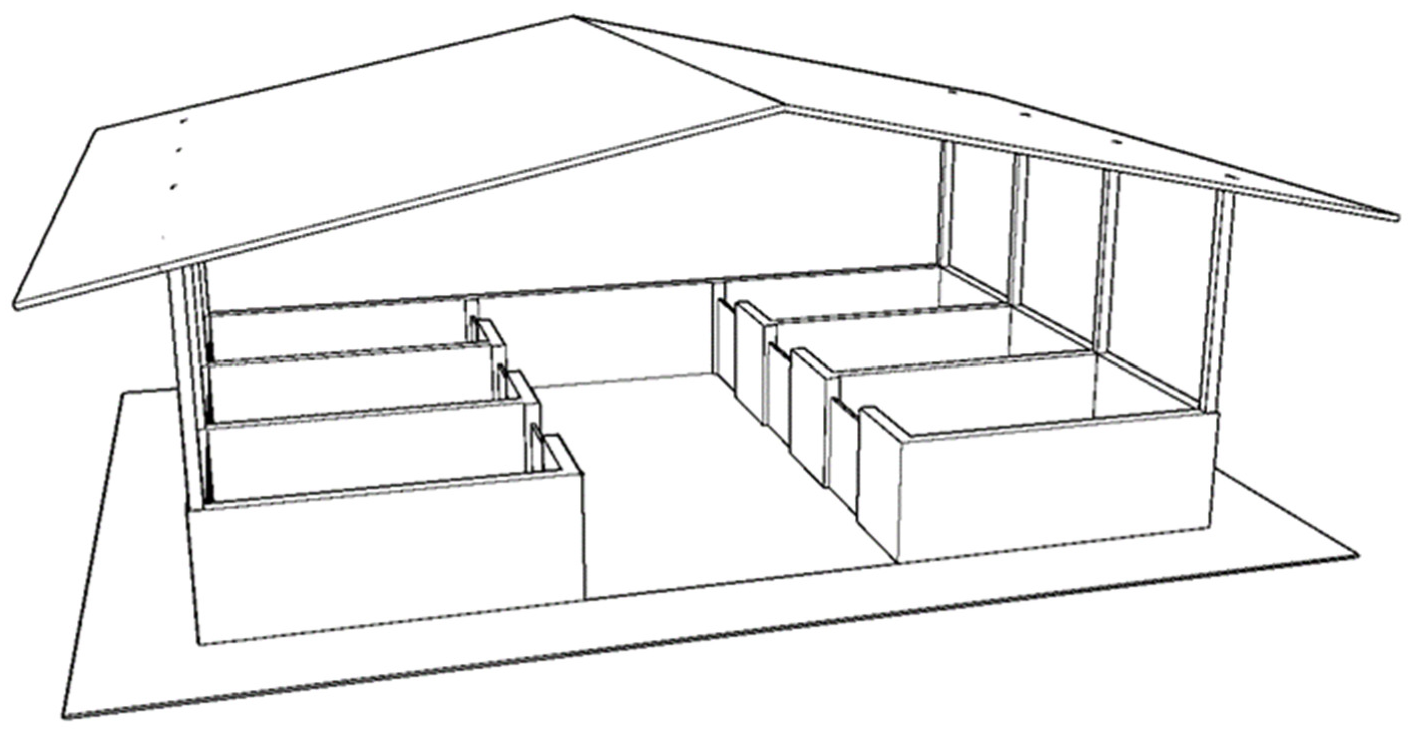
2.2. Animal Facilities

Data collection was performed from 1 August to 30 December 2018 and lasted 92 days. The experiment was approved by the CEUA/UFRPE (Ethics Committee on Animal Use) under protocol no. 23082.021090/2016-81.
The animal housing used in this study was built along the longitudinal axis in the east–west direction; the roof was covered with ceramic tiles, the walls were built of masonry, and the floor was made of concrete and had an area of 6 m2. All stalls were equipped with feeders and drinking fountains installed 30 cm from the floor. The animals received water and balanced feed appropriate to their life stages. Figure 1 illustrates the arrangement of the stalls.
Three stalls were used, one for each treatment. Different acclimatization systems were installed in the three experimental pens: three stalls were fitted with an acclimatizer to study the effect of adiabatic evaporative cooling (AEC) on the animals; three stalls were fitted with an axial fan to study the effects of forced ventilation (FV) on the animals; and the last three stalls had no acclimatization system. The animals were analyzed under natural ventilation (Con). The air conditioners used in the stalls had an average flow rate of 3 L.h−1, with independent motors and a propeller rotation of 1750 RPM, with a central disk of 3450 RPM. The flow rate of the fans was 1200 m3 h−1, at 1780 RPM, and the propeller diameter was 11″. The climate control systems were randomly distributed in the pens to reduce the influence of external factors.
We used 9 animals that were available in the university’s experimental vivarium for research, which were distributed in threes in each bay. The animals were ¾ Duroc, ¼ Pietrain commercial strains in the growth phase. The growth phase comprises the physiological phase of the animal after weaning (about 21 to 28 days), and the animal remains in this phase from 63 to 110 days of life. The average weight of the pigs was approximately 35 kg, and the ages ranged from 28 to 110 days. In terms of feeding, the pigs received a balanced and controlled diet. They were fed a combination of commercially available pig feed consisting of grains, protein sources, vitamins and minerals. The feed was carefully formulated to meet the nutritional requirements of the pigs at their respective ages and weights. Water was available throughout the experiment to ensure adequate hydration.

2.3. Meteorological Variables of the Environment

The meteorological variables collected were dry bulb temperature (Tbd; °C), relative humidity (RH, %), black globe temperature (Tgb; °C) and wind speed (Ws, m.s−1). Tbd, RH and Tgb were recorded using a HOBO® datalogger model U12-012 (Onset Computer Corporation Bourne, USA, MA,) at 08:00 and 12:00 h. The instrument was installed according to the recommendations of [33], in which it is recommended that the equipment should preferably be installed in the central region of the shed. The instrument was installed according to the recommendations of [33], in which it is recommended that the equipment should preferably be installed in the central region of the shed. The Ws (m s−1) was collected using a digital thermo-anemometer, model TAFR-180, with a scale of 0.1 to 20.0 m s−1 and a resolution of 0.1 m s−1, at 1.50 m from the ground. The measurement times were selected based on [34], the authors of which took into consideration a time with a lower temperature and a time with a higher temperature. These variables were collected inside the stalls by means of a datalogger and outside by means of a meteorological shelter, both at 1.50 m height, and were used to verify the variations between treatments. The thermal characterization of the stalls was determined through a reclassification of the BGTHI for pigs, considering the minimum optimal temperature value (15 °C), the upper critical temperature (27 °C), the average values of the thermoneutral zone for the finishing phase (15 to 18 °C) mentioned by the authors of [35] in their reference study and the relative air humidity value range of 50 to 70% cited in [36] as a basis for the reclassification of the BGTHI. These temperature and humidity values were used to estimate the dew-point temperature (DPT, °C) using the Magnus–Tetens [37] equation (Equation (1)). Subsequently, the BGTHI was estimated using the equation given in [38], which was developed for cattle.
DPT = (c × γ × (Tbd, RH))/(b − γ(Tbd, RH))
where DPT is the dew-point temperature, γ(Tbd, RH) is the intermediate result, Tbd is the temperature, RH is the relative humidity, b is a constant with a value of 238.88 and c is a constant with a value of 17.368.

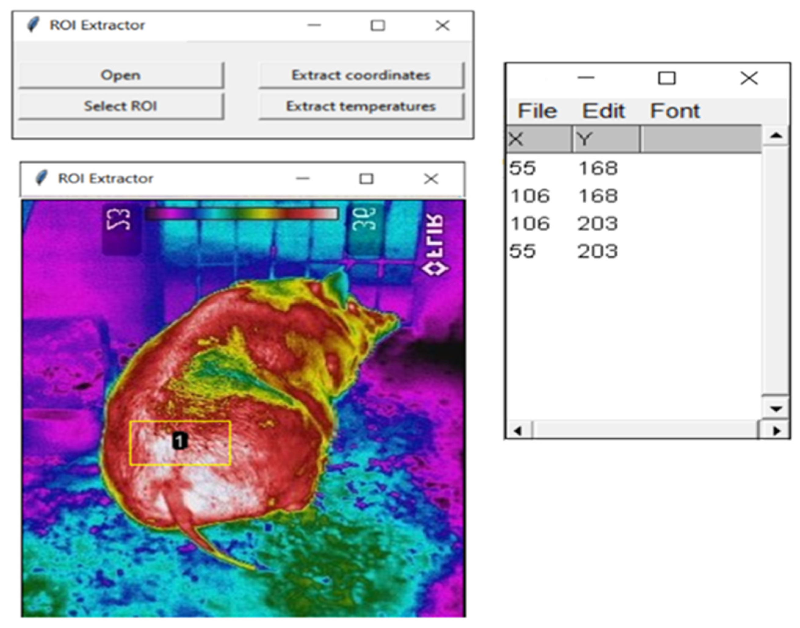
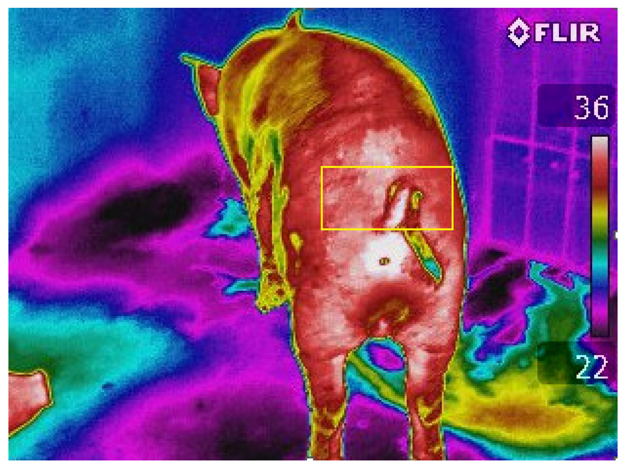
2.4. Physiological Variables of the Animals

To evaluate the effects of the different acclimatization systems on the animals’ thermal comfort, the following physiological variables were collected from the animals: rectal temperature (RT), respiratory rate (RR) and surface skin temperature (SST), at 08:00 and 12:00 h, once a week, throughout the experimental period. The RR was measured by counting the movement of the flank in 1 (one) minute, using a stopwatch, and then calculating the number of movements per minute. The animals’ body temperature was checked by means of thermal images obtained with a Flir i60 thermal imager. For thermal image registration, the camera angle was standardized, and the distance between the equipment and the animal was maintained at 1 m, as in [39,40]. The camera emissivity was set to 0.98, which is suitable for biological tissues [41], for image correction using Flir software, version 1.9.
The region selected in the animals was the dorsal–caudal region. This region in pigs was also studied by the authors of [42], who evaluated the temperatures of various body regions. Ref. [5] evaluated the welfare and surface temperatures of piglets submitted to different heating systems. Ref. [20] analyzed heat-stress indicators by means of eye temperature. Ref. [43] analyzed the influence of the environment on sow reproduction. Ref. [34] studied the body surface temperature of heifers using thermal imaging.
The extraction step for the coordinates of the selected region was performed with a software system developed in Python language with an interface using the Tkinter library. This step is of great importance for geostatistical analysis because when working with pixel-by-pixel temperatures it is necessary to know the location of each temperature value in the image.
When using the Flir software to perform image information extraction, one notices that it only extracts the temperature values as a whole or from a certain area within the image. This prompted the development of the software.
The routine used for the development consisted of importing and loading the image on the screen and opening a square, where it was moved to the desired region, considering the movement of the mouse over the image, selecting the ROI (lateral array) and displaying the coordinates of the selected window. The window was then closed and the program finished (Figure 2).
The software for extraction of the region of interest in the images was developed in Python language, using the Tkinter library to develop the interface and Opencv for analysis. Initially, by means of the “Open” button, the image is loaded from the user’s computer, which allows for its visualization—a feature developed by the function cv2.imread from the Opencv library.
After loading the image, multiple regions of interest can be selected using the “Select ROI” button, which uses the select ROIs function. Using this function in OpenCV, you can manually select precisely the areas of interest, which allows you to perform many tasks for that specific area of the image. It also makes it possible to use the specific area as input for another task, such as drawing a tracing figure (rectangle) using the coordinates or cutting the image with precision and freedom.

2.5. Statistics

The animal surface temperature data were submitted to exploratory and geostatistical analysis. The exploratory analysis included descriptive statistics and normality analysis, both performed in Excel 2016 software. The parameters determined were the mean, median, mode, standard deviation (SD), variance, coefficient of variation (CV), kurtosis, asymmetry, minimum value, maximum value and the point count. The coefficient of variation was classified according to the proposal of [44], ranging from low (CV < 12%) to medium (12% > CV < 24%) to high (CV > 24%). To study normality, the Kolmogorov–Smirnov test was used, with α = 0.05.
Geostatistics was applied according to the methodology proposed in [45] to characterize the temperature variation in the dorsal–caudal regions of the 3 animals in each of the 3 treatments at 8:00 a.m. and 12:00 p.m. We used GS+ software, version 7.0 [46] to generate the graphs.
Once the semivariograms were elaborated, the models that best fitted the data were verified. The models tested were the spherical, exponential and Gaussian models, which, according to [47], were the most relevant. To select the model that best fitted the data, the R2 value and the degree of spatial dependence (DSD) were determined through the relationship C/(C0 + C1), following the criteria recommended by [48], which classified DSD as strong spatial dependence (DSD < 25%), moderate dependence (25 ≤ DSD < 75%) and weak dependence (DSD ≥ 75%). The fitted semivariograms were selected and validated using the cross-validation criterion proposed by [49], in which it was observed whether the means and standard deviations of the errors between the observed and estimated data were close to 0 and 1, respectively—a step considered to be of great importance [50].
With the parameters of the semivariogram models selected, kriging maps were made using Surfer 13 software [51].

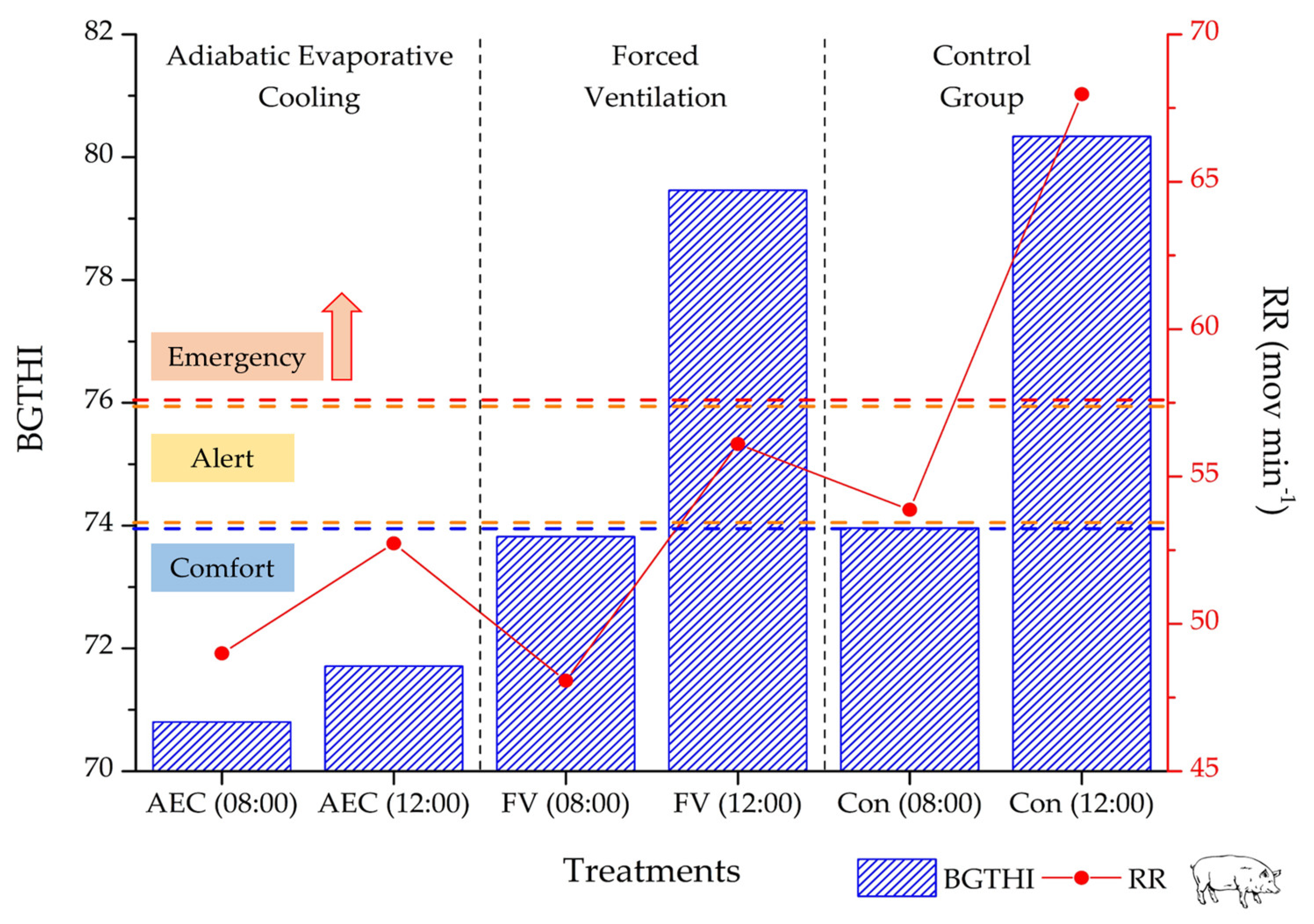
3. Results and Discussion

The characterization of the pens regarding thermal comfort at 08:00 and 12:00 h was evaluated through the classification of BGTHI for pigs developed in this study. The thermal comfort characterization of the stalls at 8 and 12 h was evaluated through the classification of the BGTHI for pigs developed in this study. The classification is presented in Table 1.
The reclassification of BGTHI for pigs took into account critical air temperature and humidity values for pigs. The threshold for the cold-stress class was the minimum optimal temperature, the threshold for the comfort class was the average of the thermoneutral zone for pigs, and the thresholds for the alert and emergency phases were based on the fragmentation of the upper critical temperature. The humidity range varied from 50 to 70%.
The BGTHI values were presented as comfortable in the pens with AEC at 8 and 12 h, ranging from 71.24 to 71.02. However, in the pens with FV, the BGTHI was evaluated as comfortable at 08:00 h, with a value of 73.69, but with stress the BGTHI reached 80.24 at 12:00 h. In the pens with Tbd, the condition was also evaluated as emergency at both time points, with a range of 73.63 to 81.43. These results were similar to those found according to the classification of [52] regarding the black globe temperature and humidity index (BGTHI) for the same facilities. The following Figure 3 presents the classification results.
As observed, the effect of high temperatures in the facilities influenced the respiratory rate of the pigs, indicating possible heat stress. In the FV and Con treatments, as the BGTHI increased, the respiratory rate of the animals also increased.
The results for Tbd and RH as functions of the environments of the treatments, of the external environment and of the times are shown in Table 2.
The ambient air temperatures and humidities in the stalls with AEC, FV and Tbd treatments at 08:00 a.m. were within the limits considered optimal for pigs in the growing phase, according to the recommendations of [52], which considered a temperature range of 20 to 27.3 °C to be comfortable for pigs in the growth phase and a temperature above 27 °C to be critical, from which it can be inferred that the animals were subjected to periods of heat stress at 12:00 p.m. However, the microclimate in the AEC treatment was already under the influence of the climate control equipment in the first hour. The microclimate of the stall with AEC had a lower value of 1.9 °C at 08:00 a.m., while in the other stalls there were no significant differences at this time. This fact shows the attenuation caused by the air conditioner, while in the stall with the fan it was not possible to detect a greater variation. However, the temperatures in this room were low due to the low solar radiation at this time.
Observing the environments, after 4 h of operation of the climatization systems, it was possible to notice, in relation to the control experiment, that the air conditioner reduced the temperature by up to 3.59 °C, while the fan operation decreased it by only 0.26 °C—a fact found by the authors of [53], who studied thermal comfort in the same facilities and found that the fan had low efficiency with respect to reducing the Tbd.
It can be seen that, in relation to the external environment, the acclimatization provided a high reduction in the Tbd in the hottest hours of the day compared with the non-acclimatized and non-shaded environment, which is favorable when dealing with pigs, which are homeothermic animals. This is explained by the characteristics of the climatizer that uses water evaporation to cool the air that circulates around the animals and reduces the temperature of the environment, providing greater thermal comfort for the pigs. According to [34], animals submitted to environments with temperatures outside the thermal comfort zone demand more energy for the maintenance of body temperature, which can affect the performance and, in more severe cases, cause the death of the animals.

Statistical Analysis

The descriptive statistics for the animals’ skin surface temperatures extracted from the thermal images and the KS test analysis are presented in Table 3 as a function of the treatments and their respective times.
The means and medians for each of the animals analyzed showed close values, which shows that the data were close to a normal distribution. Similar results were found in [6]. The coefficient of variation (CV) in statistical analyses serves as a first indicator of whether or not data heterogeneity exists. Considering the research of [44], the dorsal–caudal surface temperatures of the pigs in the three treatments showed low variability (CV < 12%), and the mean was representative. Most animals presented kurtosis and asymmetry values close to 0, except for the temperature collected at 12:00 p.m. in the AEC treatment, with values of 5.7 and −2.16, respectively. However, the Kolmogorov–Smirnov test results were not significant for all the animals analyzed.
It was observed that the animals in the stall with AEC had the lowest mean temperatures in the dorsal–caudal region (32.40 and 36.25 °C) when compared with the animals submitted to the FV treatment, which had values of 32.51, 32.59 and 36.81, and those under the Con treatment, which had values of 37.15, 37.53 and 38.45 °C, reflecting the importance of the acclimatization with AEC during the hours of 08 a.m. and 12 p.m. These results were close to those obtained by the authors of [42], who analyzed the temperatures of various body regions of pigs and found an average temperature for the caudal–dorsal region of 34.6 °C. For [54], in housing conditions within the thermoneutral zone, the skin temperature (SST) of pigs should be close to 34 ± 1 °C. Thus, the use of descriptive statistics was able to distinguish the animals submitted to the different acclimatization systems. Ref. [5] found the SSTs of pigs in concrete facilities to be similar to those recorded in this research, ranging from 39 to 41 °C. In the findings of [55], it was mentioned that body surface temperatures in the lumbar and dorsal regions have a high correlation with RT, which is considered the most suitable for evaluating temperatures in animals. Ref. [20] cited dorsal temperature as an indicator for describing the environment the animal is inhabiting.
Table 4 illustrates a proposed model fitted to the experimental data; the nugget effect, the sill, the range, the degree of spatial dependence (DSD) and the R2 value for each of the animals were analyzed.
The Gaussian model was the theoretical model with the best fit to the temperature data for the dorsal–caudal regions of the animals in all climatization systems. Such a model was validated by presenting the means between the actual values and those estimated by the model closer to zero and the standard deviation of one. According to [56], the validation of semivariograms is performed using the residuals, which is the way to check the assumptions of the model used in kriging, making the comparison between the actual values and the kriged ones, where such residuals show the performance of the model. The Gaussian model was also observed in the results of [34]—a study on the variability of body SST in cows—and in [57]—a study on the variability of udder temperature in cows.
For all the treatments analyzed, no pure nugget effect was detected, showing that there was a correlation between the different types of climatization and the SSTs of the animals; however, the results showed the low precision of the sampled grid [48]. In the AEC treatment, the nugget effect ranged from 0.51 to 0.12; in FV, the range was 0.20 to 0.03; and in Con, it was 0.01 to 0.001.
The sill indicates the point from which the samples become independent because of the distance separating them. In the facilities with AEC, the sill varied from 4.60 to 0.50. In the facilities with FV, it ranged from 0.66 to 0.10, and in the facilities with Tbd treatment, the sill ranged from 0.03 to 0.14. Similar plateau values were found in [56], which revealed that the lower the sill value, the more similar the neighboring values are.
The range indicates the distance (the region on the surface of the pig) over which the sample points (temperatures) are more similar to each other and could be used for estimating values with closer spacings than those separated by larger distances. In the AEC, the largest value was 22.60 mm at 12:00 p.m., and the smallest value was 05.10 mm at 08:00 a.m. The average value was 13.8 mm. In the FV treatment, the range was 27.20 to 43.20 mm at 08:00 a.m. and 12:00 p.m., and the average value was 35.2 mm. The Con treatment was similar to the FV treatment, with a greater range of 28.80 (08:00 a.m.) to 54.20 mm (12:00 p.m.) and an average value of 41.50 mm. The highest ranges obtained were for the Con treatment, followed by the FV treatment, and the lowest range was found for the AEC treatment.
According to the classification proposed in [48], the dorsal–caudal surface temperatures fell into the moderate-to-strong class of spatial dependence in all proposed models. This result was also found by the authors of [34], who, when studying temperature variability in cows, detected that the model with the best theoretical fit was the Gaussian model with a strong degree of spatial dependence.
The spatial variations of the temperatures analyzed in the dorsal–caudal region (Figure 4) of the animals are illustrated in Figure 5, Figure 6 and Figure 7.
These figures show the kriging maps, which are widely used in geostatistics to estimate unknown values at unsampled locations based on collected samples. In the context of the surface temperature of animals, kriging maps can be applied to estimate the spatial distribution of surface temperatures over the skin. The values estimated by kriging were similar to those found through the measurements of the authors of [39], obtained using infrared thermography in pigs, who found values ranging from 32 to 34 °C, similar to the values recorded for the animals in the AEC and FV treatments at 08:00 h in the morning. The authors of [39] also found temperature values in the caudal–dorsal region ranging from 35.8 to 37.7 °C, which were similar to the values found in this study for the animals at 12:00 h, validating the results of the kriging.
The elaborated kriging maps show the temperature distributions in the dorsal–caudal regions of the animals. Along the X- and Y-axes are the coordinates of the dorsal–caudal regions studied in millimeters. The isolines represent the estimated temperature values. These values varied from 28 to 36°C. The elaborated kriging maps showed the temperature distributions in the dorsal–caudal regions of the animals. In [24], the kriging maps also presented the distribution of air temperature values in the state of Minas Gerais. In this way, it was possible to visualize the highest temperature values in the hottest hours of the analyzed period (redder colors) in all treatments, showing the relationship between the animal’s skin temperature values and the environment.
Therefore, it can be seen that the highest temperatures found were for the animals in the stall with the Con treatment (natural acclimatization), followed by the animals in the stall with the FV treatment and, lastly, the animals in the stall with the AEC treatment. The animal housing for the Con treatment, by absorbing solar radiation in its structure, heats the microclimate, and as this, in turn, is not being influenced by air conditioning equipment capable of attenuating the temperature, it ends up heating the animal’s skin, thus increasing the temperature in the caudal–dorsal region. What happened in the FV treatment is explained by the inefficiency of the ventilator in controlling the temperature, while in the stall with AEC, the animals remained at temperatures considered optimal throughout the analyzed period, justifying the importance of acclimatization for the production environment.
In general, it was possible to visualize the information on the spatial dependence of the semivariograms expressed in the kriging maps. Such information reflects the variability in animal surface skin temperatures related to climate systems and is useful for identifying whether housings require more or less care.
Regarding the rectal temperatures of the animals subjected to AEC, the average data showed values of 38.3 °C and 38.8 °C for the animals at 08:00 and 12:00 h, respectively. The animals in the FV treatment had values of 38.5 °C and 38.7 °C at 08:00 and 12:00 h, while the animals in the control group had average values of 38.7 °C and 39.7 °C. As for the average respiratory rate, the animals in the AEC treatment had values of 49 and 52.73 breaths per minute, those in the FV treatment had values of 48.7 and 56.10 breaths per minute, and those in the Con treatment had values of 53.87 and 67.97 breaths per minute. These results indicate that the animals under the effect of the air conditioner showed lower physiological values compared to the other animals, with lower respiratory rates.

4. Conclusions

The results show that thermal imaging and geostatistical analysis are able to provide valuable information about the thermal behavior of pigs and the characteristics of their environments. Furthermore, a combination of these tools contributes to the implementation of appropriate management measures and the improvement of animal welfare. The geostatistical analysis provided a mathematical model capable of illustrating the variation in temperature in the caudal–dorsal regions of the pigs according to the environments to which the animals were subjected, showing the potential of these tools for monitoring the body temperature of pigs in different environments and combining this data with information on spatial variability transmitted by geostatistical analysis.
The work highlights the importance of using thermal imaging and geostatistics in animal production, highlighting their potential to provide accurate and auxiliary information on animal performance and welfare, as well as to assist in decision making regarding production management. The use of these tools can contribute significantly to the promotion of more sustainable and efficient practices in animal production, benefiting both producers and consumers.

Author Contributions

Conceptualization, M.d.F.A.A. and H.P.; methodology, A.A.d.A.M.; software, R.A.B.d.S.; validation, N.F.G., T.C.S. and G.L.P.d.A.; formal analysis, G.T.B.M.; investigation, M.V.d.S.; resources, W.A.d.S.; data curation, M.V.d.S.; writing—original draft preparation, T.C.S.; writing—review and editing, T.C.S.; visualization, H.P.; supervision, M.V.d.S.; project administration, M.d.F.A.A.; funding acquisition, T.C.S. All authors have read and agreed to the published version of the manuscript.

Funding

This research received no external funding.

Institutional Review Board Statement

The research was approved by the CEUA/UFRPE (Animal Ethics Committee) under protocol number 23082.021090/2016-81, date of license issuance: 5 December 2016.

Informed Consent Statement

Not applicable.

Data Availability Statement

Not applicable.

Acknowledgments

The authors wish to acknowledge the Programa de Pós-Graduação em Engenharia Agrícola (PGEA) and the Grupo de Pesquisa em Ambiência (GPESA) of the Universidade Federal Rural de Pernambuco (UFRPE) for the necessary support for the development of this study. The authors would also like to acknowledge the Coordenação para o Aperfeiçoamento do Pessoal do Ensino Superior (CAPES—Financial Code 001) and the Fundação de Apoio à Investigação do Estado de Pernambuco (FACEPE) for the provision of research scholarships.

Conflicts of Interest

The authors declare no conflict of interest.

References

  1. ABPA. Relatório Anual 2021. Available online: https://abpa-br.org/quem-somos/abpa-relatorio-anual/ (accessed on 24 March 2021).
  2. Embrapa Embrapa Suínos e Aves. Available online: https://www.embrapa.br/suinos-e-aves/cias/estatisticas (accessed on 1 March 2022).
  3. Galvão, A.T.; da Silva, A.d.S.L.; Pires, A.P.P.; de Morais, Á.F.F.; Mendonça Neto, J.S.N.; de Azevedo, H.H.F. Bem-Estar Animal na Suinocultura: Revisão. Pubvet 2019, 13, 148. [Google Scholar] [CrossRef]
  4. OIE. Terrestrial Animal Health Code. Available online: https://www.oie.int/en/standard-setting/terrestrial-code/access-online (accessed on 6 March 2021).
  5. Damasceno, F.A.; Magela Soares, C.; Eduardo, C.; Oliveira, A.; Freire, L.; Damasceno, B.; Ferreira, P.; Ferraz, P. Evaluation of Behavior in Piglets Using Digital Image Processing. Energ. Agric. 2019, 34, 217–229. [Google Scholar] [CrossRef]
  6. Medeiros, B.B.; Moura, D.J.D.; Massari, J.M.; Curi, T.M.D.C.; Maia, A.P.D.A. Uso da Geoestatística na Avaliação de Variáveis Ambientais em Galpão de Suínos Criados Em Sistema” Wean to Finish” Na Fase de Terminação. Eng. Agríc. 2014, 34, 800–811. [Google Scholar] [CrossRef] [Green Version]
  7. Soares, E.A.; Leal, A.F.; Malheiros Filho, J.R.; Camerini, N.L.; Nascimento, J.W.B.; Dermeval, A.F. Zoneamento Bioclimático Para Produção de Suínos na Maternidade no Município de Areia—PB. Available online: https://www.confea.org.br/sites/default/files/uploads-imce/Contecc2019/Agronomia/DIAGNOSTICO%20BIOCLIMATICO%20PARA%20PRODU%C3%87%C3%83O%20DE%20SUINOS%20NO%20MUNICIPIO%20DE%20AREIA-PB.pdf (accessed on 29 March 2023).
  8. Borges, P.H.M.; de Mendoza, Z.M.S.H.; Morais, P.H.M.; dos Santos, R.L. Artificial Neural Networks for Predicting Animal Thermal Comfort. Eng. Agríc. 2018, 38, 844–856. [Google Scholar] [CrossRef] [Green Version]
  9. dos Santos, T.C.; Carvalho, C.D.C.S.; da Silva, G.C.; Diniz, T.A.; Soares, T.E.; Moreira, S.d.J.M.; Cecon, P.R. Influência do Ambiente Térmico no Comportamento e Desempenho Zootécnico de Suínos. Rev. Ciênc. Agroveter. 2018, 17, 241–253. [Google Scholar] [CrossRef]
  10. Pandorfi, H.; Almeida, G.L.P.; Guiselini, C. Zootecnia de Precisão: Princípios Básicos e Atualidades na Suinocultura. Rev. Bras. Saúde Produção Anim. 2012, 13, 558–568. [Google Scholar] [CrossRef]
  11. Pandorfi, H.; Da Silva, I.J.O.; Piedade, S.M.S. Conforto Térmico para Matrizes Suínas em Fase de Gestação, Alojadas em Baias Individuais e Coletivas. Rev. Bras. Eng. Agríc. Ambient. 2008, 12, 326–332. [Google Scholar] [CrossRef]
  12. Thom, E.C. The Discomfort Index. Weatherwise 1959, 12, 57–61. [Google Scholar] [CrossRef]
  13. Buffington, D.E.; Collazo-Arocho, A.; Canton, G.H.; Pitt, D.; Thatcher, W.W.; Collier, R.J. Black Globe-Humidity Index (BGHI) as Comfort Equation for Dairy Cows. Trans. ASAE 1981, 24, 711–714. [Google Scholar] [CrossRef]
  14. Esmay, M.L. Principles of Animal Environment, 2nd ed.; American Society of Agricultural Engineers: St. Joseph, MI, USA, 1982. [Google Scholar]
  15. Albright, L.D. Environment Control for Animals and Plants; American Society of Agricultural Engineers: St. Joseph, MI, USA, 1990; Volume 4. [Google Scholar]
  16. Nasirahmadi, A.; Hensel, O.; Edwards, S.A.; Sturm, B. A New Approach for Categorizing Pig Lying Behaviour Based on a Delaunay Triangulation Method. Animal 2017, 11, 131–139. [Google Scholar] [CrossRef] [Green Version]
  17. Castro, J.D.O.; Campos, A.T.; Ferreira, R.A.; Júnior, T.Y.; Tadeu, H.C. Uso de Ardósia na Construção de Celas de Maternidade: I—Efeito Sobre o Ambiente e Comportamento de Suínos. Eng. Agríc. 2011, 31, 458–467. [Google Scholar] [CrossRef]
  18. Villa, F.; Nivaldo, A.; Junior, K.; De Oliveira, C.C. Aplicações Da Termografia Por Infravermelho (TIV) Na Bovinocultura de Corte; Repositorio de Información Tecnológica de Embrapa: Brasília, Brazil, 2020. [Google Scholar]
  19. Warriss, P.D.; Pope, S.J.; Brown, S.N.; Wilkins, L.J.; Knowles, T.G. Estimating the Body Temperature of Groups of Pigs by Thermal Imaging. Vet. Rec. 2006, 158, 331–334. [Google Scholar] [CrossRef] [PubMed]
  20. Pulido-Rodríguez, L.F.; Titto, E.A.L.; Henrique, F.L.; Longo, L.S.; Hooper, H.B.; Pereira, T.L.; Pereira, A.M.F.; Titto, C.G. Infrared Thermography of the Ocular Surface as Stress Indicator for Piglets Postweaning. Pesqui. Vet. Bras. 2017, 37, 453–458. [Google Scholar] [CrossRef] [Green Version]
  21. Vieira, F.M.; Gouveia, A.B.V.S.; de Paulo, L.M.; Sampaio, S.A.; Borges, K.F.; da Silva, N.F.; dos Santos, F.R.; Minafra, C.S. Termografia infravermelha na avicultura. Veter. Zootec. 2022, 29, 1–21. [Google Scholar] [CrossRef]
  22. da Silva, T.C.S.; Mariz, T.M.d.A.; Escodro, P.B. Use of Thermography in Clinical and Sports Evaluations of Equine Animals: A Review. Res. Soc. Dev. 2022, 11, e13911530532. [Google Scholar] [CrossRef]
  23. Cardoso, L.A.S.; Farias, P.R.d.S.; Soares, J.A.C. Geoestatística Aplicada à Fitossanidade: Estado da Arte e Perspectivas Futuras para o Estado do Pará, Brasil. Available online: https://www.journalijdr.com/geoestat%C3%ADstica-aplicada-%C3%A0-fitossanidade-estado-da-arte-e-perspectivas-futuras-para-o-estado-do-par%C3%A1 (accessed on 29 March 2023).
  24. Viana, R.S.M.; dos Santos, G.R.; Moreira, D.S.; Louzada, J.M.; Rosa, L.M.F. O Uso da Geoestatística Espaço-Temporal na Predição da Temperatura Máxima do Ar. Rev. Bras. Geogr. Fís. 2019, 12, 96–111. [Google Scholar] [CrossRef]
  25. Marques, S.d.F.; Pitombo, C.S. Intersecting Geostatistics with Transport Demand Modeling: A Bibliographic Survey. Rev. Bras. Cartogr. 2020, 72, 1004–1027. [Google Scholar] [CrossRef]
  26. Da Silva, H.M.; Sarnighausen, V.C.R. Análise Geoestatística de Séries Temporais de Temperatura do Ar, Evapotranspiração de Referência e Precipitação Pluvial. Rev. Ibero-Am. Ciênc. Ambient. 2021, 12, 710–717. [Google Scholar] [CrossRef]
  27. Silva Neto, S.P.; Silva, R.G.; Santos, A.C.; Gama, F.R.; Guerra, M.S.S.; Brito, M.J.D. Padrões Espaciais de Deposição de Fezes por Bovinos de Corte Em Áreas de Pastagem. Rev. Bras. Saúde Produção Anim. 2011, 12, 538–550. [Google Scholar]
  28. Nääs, I.D.A.; Garcia, R.G.; Graciano, D.E.; De Santana, M.R.; Caldara, F.R.; Dourados, G. Temperatura Superficial de Porcas em Lactação Submetidas ao Resfriamento Adiabático. Encicl. Biosf. 2013, 9, 2006–2013. [Google Scholar]
  29. Jia, G.; Li, W.; Meng, J.; Tan, H.; Feng, Y. Non-Contact Evaluation of Pigs’ Body Temperature Incorporating Environmental Factors. Sensors 2020, 20, 4282. [Google Scholar] [CrossRef] [PubMed]
  30. Basak, J.K.; Okyere, F.G.; Arulmozhi, E.; Park, J.; Khan, F.; Kim, H.T. Artificial Neural Networks and Multiple Linear Regression as Potential Methods for Modelling Body Surface Temperature of Pig. J. Appl. Anim. Res. 2020, 48, 207–219. [Google Scholar] [CrossRef]
  31. Bezerra, A.C.; da Silva, J.L.B.; Silva, D.A.d.O.; Batista, P.H.D.; Pinheiro, L.d.C.; Lopes, P.M.O.; Albuquerque, G.B. Monitoramento Espaço-Temporal da Detecção de Mudanças em Vegetação de Caatinga por Sensoriamento Remoto no Semiárido Brasileiro. Rev. Bras. Geogr. Fís. 2020, 13, 286–301. [Google Scholar] [CrossRef]
  32. Jardim, A.M.d.R.F.; de Queiroz, M.G.; Júnior, G.D.N.A.; da Silva, M.J.; da Silva, T.G.F. Estudos Climáticos Do Número de Dias de Precipitação Pluvial para o Município de Serra Talhada-PE. Rev. Eng. Agric.—REVENG 2019, 27, 330–337. [Google Scholar] [CrossRef]
  33. Barbosa Filho, J.A.D.; Silva, I.J.O.; Silva, M.A.N.; Silva, C.J.M. Avaliação Dos Comportamentos de Aves Poedeiras Utilizando Seqüência de Imagens. Eng. Agríc. 2007, 27, 93–99. [Google Scholar] [CrossRef] [Green Version]
  34. Batista, P.H.D.; de Almeida, G.L.P.; Pandorfi, H.; da Silva, M.V.; da Silva, R.A.B.; da Silva, J.L.B.; Santana, T.C.; Rodrigues, J.A.d.M. Thermal Images to Predict the Thermal Comfort Index for Girolando Heifers in the Brazilian Semiarid Region. Livest. Sci. 2021, 251, 104667. [Google Scholar] [CrossRef]
  35. Baêta, F.C.; Souza, S.C. Ambiência Em Edificações Rurais—Conforto Animal; UFV: Abbotsford, BC, Canada, 1997; Volume 246. [Google Scholar]
  36. Campos, J.A.; Tinôco, I.d.F.F.; Baêta, F.d.C.; Cecon, P.R.; Mauri, A.L. Air Quality, Thermal Environment and Performance of Pigs Raised in Nurseries with Different Dimensions. Agric. Eng. 2009, 29, 339–347. [Google Scholar] [CrossRef] [Green Version]
  37. Lawrence, M.G. The Relationship between Relative Humidity and the Dewpoint Temperature in Moist Air: A Simple Conversion and Applications. Bull. Am. Meteorol. Soc. 2005, 86, 225–233. [Google Scholar] [CrossRef]
  38. Teixeira, D.L.; Boyle, L.A.; Enríquez-Hidalgo, D. Skin Temperature of Slaughter Pigs With Tail Lesions. Front. Vet. Sci. 2020, 7, 198. [Google Scholar] [CrossRef]
  39. Moreira, V.E.; Veroneze, R.; Teixeira, A.D.R.; Campos, L.D.; Lino, L.F.L.; Santos, G.A.; Silva, B.A.N.; Campos, P.H.R.F. Effects of Ambient Temperature on the Performance and Thermoregulatory Responses of Commercial and Crossbred (Brazilian Piau Purebred Sires × Commercial Dams) Growing-Finishing Pigs. Animals 2021, 11, 3303. [Google Scholar] [CrossRef]
  40. Mostaço, G.M.; Miranda, K.O.D.S.; da S Condotta, I.C.F.; Salgado, D.D. alessandro Determination of Piglets’ Rectal Temperature and Respiratory Rate through Skin Surface Temperature under Climatic Chamber Conditions. Eng. Agric. 2015, 35, 979–989. [Google Scholar] [CrossRef] [Green Version]
  41. Rauber, S.M. Termografia Infravermelho na Avaliação de Estratégias de Alimentação de Precisão Para Suínos; LUME: Porto Alegre, Brazil, 2016. [Google Scholar]
  42. Nääs, I.d.A. A Iinfluência do Meio Ambiente na Reprodução. In Proceedings of the Simpósio Internacional de Suinocultura, São Paulo, Brazil, 9–12 July 2000. [Google Scholar]
  43. Warrick, A.W.; Nielsen, D.R. Spatial Variability of Soil Physic Properties in the Field. N. Y. Acad. 1980, 655–675. [Google Scholar] [CrossRef] [Green Version]
  44. Vieira, S.R. Geoestatística em Estudos de Variabilidade Espacial do Solo. Tópicos Ciência Solo. Viçosa Soc. Bras. Ciência Solo 2000, 1, 1–54. [Google Scholar]
  45. Gamma Design Software GS+—Geostatistics for the Environmental Sciences; Gamma Design Software: Plainwell, MI, USA, 2012; Available online: http://www.gammadesign.com/ (accessed on 16 October 2022).
  46. Obroślak, R.; Dorozhynskyy, O. Selection of a Semivariogram Model in the Study of Spatial Distribution of Soil Moisture. J. Water Land Dev. 2017, 35, 161–166. [Google Scholar] [CrossRef] [Green Version]
  47. Cambardella, C.A.; Moorman, T.B.; Novak, J.M.; Parkin, T.B.; Karlen, D.L.; Turco, R.F.; Konopka, A.E. Field-Scale Variability of Soil Properties in Central Iowa Soils. Soil Sci. Soc. Am. J. 1994, 58, 1501–1511. [Google Scholar] [CrossRef]
  48. Vauclin, M.; Vieira, S.R.; Vachaud, G.; Nielsen, D.R. The Use of Cokriging with Limited Field Soil Observations. Soil Sci. Soc. Am. J. 1983, 47, 175–184. [Google Scholar] [CrossRef]
  49. Santarosa, L.V.; Manzione, R.L. Soil Variables as Auxiliary Information in Spatial Prediction of Shallow Water Table Levels for Estimating Recovered Water Volume. RBRH 2018, 23, e24. [Google Scholar] [CrossRef] [Green Version]
  50. Golden Software. Golden Software Surfer for Windows: Realese 7.0, Contouring and 3D Surface Mapping for Scientist’s Engineers User’s Guide; Golden Software: Golden, CO, USA, 2016. [Google Scholar]
  51. Rinaldo, D.; Le Dividich, J.; Noblet, J. Adverse Effects of Tropical Climate on Voluntary Feed Intake and Performance of Growing Pigs. Livest. Prod. Sci. 2000, 66, 223–234. [Google Scholar] [CrossRef]
  52. Gomes, N.F.; Barnabe, J.M.C.; Silva, W.A.; Pandorfi, H.; Guiselini, C.; Almeida, G.L.P. Acondicionamento Térmico para Suínos na Fase de Crescimento no Semiárido Pernambucano. In Proceedings of the Simpósio Internacional de Ambiência e Engenharia na Produção Animal; Simpósio Internacional de Ambiência e Engenharia na Produção Animal, Lavras, Brazil, 5–7 June 2019. [Google Scholar]
  53. Malmkvist, J.; Pedersen, L.J.; Kammersgaard, T.S.; Jørgensen, E. Influence of Thermal Environment on Sows around Farrowing and during the Lactation Period. J. Anim. Sci. 2012, 90, 3186–3199. [Google Scholar] [CrossRef]
  54. Magano, D.A.; Machado, M.R.R.; Jerónimo, J.A.; Guedes, J.V.C.; Doberstein, A.P.S. Modelagem Geostatistica Aplicada a Distribuição Espacial de Lagartas Presentes na Cultura da Soja. Braz. J. Anim. Environ. Res. 2023, 6, 20–29. [Google Scholar] [CrossRef]
  55. da Silva, R.Â.B.; Pandorfi, H.; de Almeida, G.L.P.; de Assunção Montenegro, A.A.; da Silva, M.V. Spatial Dependence of Udder Surface Temperature Variation in Dairy Cows with Healthy Status and Mastitis. Rev. Bras. Saude Prod. Anim. 2019, 20. [Google Scholar] [CrossRef]
  56. de Carvalho, J.R.P.; Assad, E.D.; Evangelista, S.R.M.; Pinto, H.D.S. Estimation of Dry Spells in Three Brazilian Regions—Analysis of Extremes. Atmos. Res. 2013, 132–133, 12–21. [Google Scholar] [CrossRef]
  57. Ricci, G.D.; da Silva-Miranda, K.O.; Titto, C.G. Infrared Thermography as a Non-Invasive Method for the Evaluation of Heat Stress in Pigs Kept in Pens Free of Cages in the Maternity. Comput. Electron. Agric. 2019, 157, 403–409. [Google Scholar] [CrossRef]
Figure 1. Structure of the animal facilities used in this study. Source: The authors.
Agriengineering 05 00069 g001
Figure 2. Interface developed for extracting the coordinates from the thermal image. Note: The number 1 represents a point sampled in the caudal dorsal region.
Agriengineering 05 00069 g002
Figure 3. Classification of BGTHI in animal premises.
Agriengineering 05 00069 g003
Figure 4. Dorsal–caudal region studied.
Agriengineering 05 00069 g004
Figure 5. Kriging maps of the dorsal–caudal region for the AEC treatment at 8:00 a.m. and 12:00 p.m.
Agriengineering 05 00069 g005
Figure 6. Kriging maps of the dorsal–caudal region for the FV treatment at 08:00 a.m. and 12:00 p.m.
Agriengineering 05 00069 g006
Figure 7. Kriging maps of the dorsal–caudal region for the T treatment at 08:00 a.m. and 12:00 p.m.
Agriengineering 05 00069 g007
Table 1. BGTHI reclassification for pigs.
ClassInterval
Cold stressBGTHI ≤ 67
Comfort68 < BGTHI ≤ 74
Alert74 < BGTHI ≤ 76
EmergencyBGTHI > 76
Table 2. Temperatures and humidities of the air inside the pens and in the external environment.
TimeAECFVTbdExternal Environment
Tbd °CRH%Tbd °CRH%Tbd °CRH%Tbd °CRH%
08:00 a.m.22.9670.724.8767.9324.6372.524.4465.25
12:00 p.m.29.4690.532.7942.0633.0547.2933.3139.07
Table 3. Descriptive statistics for dorsal–caudal surface temperatures of the pig.
TreatmentTimeMeanMedianSDCVKustosisAsymmetryKS
AEC08:00 a.m.32.4032.62.216.81−1.34−0.200.36
AEC12:00 p.m.36.2536.440.732.005.7−2.160.30
FV08:00 a.m.32.5132.891.033.17−1.34−0.410.28
FV12:00 p.m.36.8136.800.170.480.800.320.40
Con08:00 a.m.37.5337.570.250.68−0.79−0.080.24
Con12:00 p.m.38.4538.530.280.730.42−1.030.29
Table 4. Semivariogram parameters.
TreatmentsTimeModelsNugettSillRangeDSDR2
AEC08:00 a.m.Gaussian0.5104.60005.10087.8000.810
AEC12:00 p.m.Gaussian0.1200.50022.60075.5000.930
FV08:00 a.m.Gaussian0.2001.66027.45098.8000.980
FV12:00 p.m.Gaussian0.0300.10043.20099.2300.990
Con08:00 a.m.Gaussian0.0100.03028.80071.6000.970
Con12:00 p.m.Gaussian0.0030.14054.20097.7400.990
Disclaimer/Publisher’s Note: The statements, opinions and data contained in all publications are solely those of the individual author(s) and contributor(s) and not of MDPI and/or the editor(s). MDPI and/or the editor(s) disclaim responsibility for any injury to people or property resulting from any ideas, methods, instructions or products referred to in the content.

