Article

Delineating Management Zones with Different Yield Potentials in Soybean–Corn and Soybean–Cotton Production Systems

by
Eduardo Antonio Speranza
1,*,
João de Mendonça Naime
2,
Carlos Manoel Pedro Vaz
2,
Júlio Cezar Franchini dos Santos
3,
Ricardo Yassushi Inamasu
2,
Ivani de Oliveira Negrão Lopes
3,
Leonardo Ribeiro Queirós
1,
Ladislau Marcelino Rabelo
2,
Lucio André de Castro Jorge
2,
Sergio das Chagas
4,
Mathias Xavier Schelp
5 and
Leonardo Vecchi
5
1
Brazilian Agricultural Research Corporation, Embrapa Digital Agriculture, Campinas 13083-886, SP, Brazil
2
Brazilian Agricultural Research Corporation, Embrapa Instrumentation, São Carlos 13560-970, SP, Brazil
3
Brazilian Agricultural Research Corporation, Embrapa Soybean, Londrina 86085-981, PR, Brazil
4
Amaggi Group, Sapezal 78365-000, MT, Brazil
5
Robert Bosch Limitada, Campinas 13012-970, SP, Brazil
*
Author to whom correspondence should be addressed.
Submission received: 14 June 2023 / Revised: 19 August 2023 / Accepted: 24 August 2023 / Published: 31 August 2023
(This article belongs to the Special Issue Big Data Analytics in Agriculture)

Abstract

:
The delineation of management zones is one of the ways to enable the spatially differentiated management of plots using precision agriculture tools. Over the years, the spatial variability of data collected from soil and plant sampling started to be replaced by data collected by proximal and orbital sensors. As a result, the variety and volume of data have increased considerably, making it necessary to use advanced computational tools, such as machine learning, for data analysis and decision-making support. This paper presents a methodology used to establish management zones (MZ) in precision agriculture by analyzing data obtained from soil sampling, proximal sensors and orbital sensors, in experiments carried out in four plots featuring soybean–cotton and soybean–corn crops, in Mato Grosso and Paraná states, Brazil. Four procedures were evaluated, using different input data sets for the MZ delineation: (I) soil attributes, including clay content, apparent electrical conductivity or fertility, along with elevation, yield maps and vegetation indices (VIs) captured during the peak crop biomass period; (II) soil attributes in conjunction with VIs demonstrating strong correlations; (III) solely VIs exhibiting robust correlation with soil attributes and yield; (IV) VIs selected via random forests to identify the importance of the variable for estimating yield. The results showed that the VIs derived from satellite images could effectively replace other types of data. For plots where the natural spatial variability can be easily identified, all procedures favor obtaining MZ maps that allow reductions of 40% to 70% in yield variance, justifying their use. On the other hand, in plots with low natural spatial variability and that do not have reliable yield maps, different data sets used as input do not help in obtaining feasible MZ maps. For areas where anthropogenic activities with spatially differentiated treatment are already present, the exclusive use of VIs for the delineation of MZs must be carried out with reservations.

Graphical Abstract

1. Introduction

The natural spatial variability of soil and crop attributes within an agricultural plot can be identified from data collected by different types of sensing, which include proximal, orbital, invasive or non-invasive methods. Several studies in the literature indicate that maps of attributes associated with soil genesis, such as texture and electrical conductivity; indicators plant growth and development, such as vegetation indices extracted from images; and yield maps themselves are the main sources of information for identifying this variability [1,2,3]. Nonetheless, caution must be exercised when using data collected during periods marked by spatially differentiated interventions within the field. This is because this type of data may no longer reflect the natural variability of the crop.
By analyzing individual factors, we can create maps for specific interventions at varying rates in the field. Yield maps can then be generated to determine NPK (nitrogen, phosphorus and potassium) application for the next season based on plant export rates [4]. Soil texture and electrical conductivity maps can aid in planting operations by providing insight into the appropriate seed populations for different areas [5]. Additionally, maps based on vegetation indices (VI) have been used as inputs for the development of models for estimating yield in crops such as corn [6] and sugarcane [7].
The concept of management zones (MZs) has emerged as a means to identify the various factors that can limit crop yield in an integrated manner. MZs are subdivisions of a plot into smaller areas, enabling the recognition of distinct regions with varying yield potentials, often requiring tailored treatments [8]. The primary definitions of MZs in the literature suggest that, once defined, these subdivisions should remain consistent over time and, as such, must be delineated using data that reflect the crop’s natural spatial variability [9]. Therefore, they become highly specialized sub-plots that enable the farmers to make goal-oriented decisions.
Despite MZ maps being a simplified approach for spatially differentiated plot management, their acquisition is not straightforward. Usually, the farmer does not have a precise and time-stable delineation. Thus, attributes that can indicate the natural spatial variability of the crop, such as those already mentioned, are of great importance in this process. The MZ delineation process requires the use of more complex methodologies than those used to create application maps. In this case, we should consider multivariate analysis tools that allow us to identify a data-driven natural spatial variability of the crop. In this context, unsupervised machine learning algorithms, such as clustering, have been widely used [8].
Although the clustering process is pivotal in delineating MZs, it requires pre-processing the data intended for cluster identification, which will ultimately contribute to the creation of potential MZs. In addition to employing conventional statistical tools, such as histogram analysis to detect and exclude anomalous values, it is necessary to ensure that the attributes are available in the same spatial grid. To standardize the grid, spatial interpolation algorithms like the inverse distance weighted (IDW) and the kriging geostatistical algorithm are typically used. The work of Santos and Saraiva [10] established a reference model for the process of MZ delineation, which comprises five key steps. The first step is data collection, which requires defining data type and determining appropriate sampling methods and strategies. The second step involves data filtering, during which samples with positioning errors or spurious values should be excluded. The third step is the data selection, which consists of grid standardization, normalizing attributes and removing redundant ones. Next, data clustering analysis using appropriate algorithms is performed. Finally, the last step is evaluating the maps using statistical tools to help the user to choose the best map that meets their expectations regarding operating procedures.
Considering the process reported above, Reyes et al. [11] delineated management zones for a corn experimental plot combining soil fertility, texture and electrical conductivity attributes, in addition to VIs collected in three different periods of the crop cycle. The results obtained showed the need to subdivide a plot with considerable spatial variability and the impacts that this subdivision can cause in increasing crop yield. Similarly, Ali et al. [3] included in this set of attributes average yield values obtained over seven years in a cereal crop. The results showed that the merging soil data, vegetation indices and yield resulted in two management zones (with high and low yield) having a high correlation with the attributes used to obtain them. Georgi et al. [12] developed a methodology based only on remote sensing data for the delineation of management zones when field data are not available. The proposed method offers a quick result, particularly if yield maps are not available. Therefore, some limitations were observed, such as the need to exclude images due to clouds in critical periods of the crop. The exclusive use of VIs for delineating management zones can also be observed in more recent works. Leo et al. [13] used NDVI data from the RapidEye satellite to delineate MZs for a model that simulates obtaining the best nitrogen application rates for cotton plots. The results showed that, although the obtained MZs are consistent with the NDVI, soil variability within the zones is still high. Maia et al. [14] evaluated the ability of the Vis’ NDVI and EVI2 to delineate MZs in sugarcane crops, regarding different phenological stages of the crop. As a result, the authors identified that EVI2 values from sugarcane aged from 180 to 240 days in the rainy season are the most appropriate attributes for delineating MZs in sugarcane. Finally, with a focus on the analysis of clustering algorithms, Gavioli et al. [8] performed experiments in three areas of soybean production using 17 different algorithms. Although some algorithms performed better than others considering statistical tests, the results did not indicate that these could be considered optimal for any culture or dataset used as input.
This paper presents a data-driven methodology for delineating MZs with varying yield potentials in the soybean–corn and soybean–cotton farm production. The methodology was applied to three plots with soybean and cotton crops, and one plot with soybean and corn crops. In contrast to the existing literature, this study conducted experiments in plots with diverse crop rotations during both winter and summer seasons. In addition, different combinations of vegetation indices were used exclusively, collectively and in substitution for soil and crop attributes collected in the field. The results indicate that most of the scenarios studied showed significant reduction in the yield variance when the MZs are considered, in comparison with the yield variance observed for the whole plot (without considering the MZs subdivision). For these scenarios, the application of inputs with specific rates for each MZ can be recommended to improve the management of inputs, providing greater profit to the farmer at the end of the cycle.

2. Materials and Methods

This section describes the experimental plots, types of collected data and computational and statistical tools used in this experiment.

2.1. Experimental Plots

The experiments to validate the proposed methodology in this paper were carried out in four agricultural plots situated in different regions. The first two plots (A and B), consist of production areas totaling 202 and 267 hectares, respectively, and are used for the cultivation of annual crops. Specifically, soybeans are grown as the first crop during the summer, followed by cotton as the second crop during the winter. These plots are located at the Tucunaré Farm, in Sapezal, Mato Grosso, Brazil, with central geographic coordinates of 12°59′22″ S (latitude) and 58°45′51″ W (longitude). Plot C, located at the Tanguro Farm, in Querência, Mato Grosso, Brazil, with central geographic coordinates of 12°34′12″ S (latitude) and 52°12′48″ W (longitude), has a plot of 156 hectares and shares the same configuration of annual crops and growing seasons as plots A and B. Lastly, plot D spans an area of 195 hectares and is used for the cultivation of annual crops, namely soybeans during the summer and corn during the winter. It is situated at Cachoeira Farm, in Arapongas, Parana, Brazil, with central geographic coordinates of 23°25′12″ S (latitude) and 51°25′31″ (longitude). Figure 1 shows a general location map of the experimental plots, and Figure 2 shows terrestrial images of two of the experimental plots used in this work, considering the phenological stages of flower buds (cotton) and bolting (corn).

2.2. Data Sets

Soil parameter datasets, elevation and historical yield attributes were acquired for all plots, using both proximal sensing and soil sampling. Table 1 describes some information about these attributes.
The attributes displayed in Table 1 were collected by sensors or processes performed directly in the field by each farm technical team. To achieve the number of samples per hectare, mean and standard deviation described in Table 1, the data underwent filtering processes to eliminate outliers, based on individual histogram analyses. Afterward, the spatial grids of all attributes were standardized to match the Sentinel-2 satellite grid (10 m/pixel). Images were collected using this grid to generate vegetation indices, which were also used as attributes and are described in Section 2.2. To standardize the grid, a kriging algorithm was used in attributes with few sampling densities, but with spatial dependence, while attributes with high sample density were standardized using the inverse distance weighting (IDW) method. For plots A, B and D, with the aim of mitigating distinct climatic events that may occur throughout the crop cycles, average yield maps were obtained regarding the two crops cultivated in each plot. The individual yield maps have the same measurement unit (ton/ha), but with different orders of magnitude regarding the different cultures. In this way, the individual yield maps were all standardized with values in (–1, 1) interval before obtaining the average yield maps. Thereby, for each plot, a single attribute of average yield was used, except for field C, which had only a cotton yield map in 2022.

2.3. Vegetation Indices Data Sets

The enhanced vegetation index (EVI) [15] and the normalized difference vegetation index (NDVI) [16] are widely used in the literature to identify the spatial variability of agricultural areas [17]. In a preliminary work regarding VI time series, we identified that for soybean–cotton production systems, the EVI obtained in the peak period of crop biomass can better display the spatial variability of the plot in comparison with the commonly used NDVI. On the other hand, for soybean–corn production systems, the NDVI proved to be more suitable, especially when consolidated maps are obtained separately for the summer and winter periods. Therefore, for plots A and B, the VI attributes were average maps of EVI collected from Sentinel-2 for four different dates, corresponding to the vegetative peak of each cotton or soybean cycle where yield maps were available. For plot C, an EVI map obtained in a specific biomass peak date was used, as there was only one yield map available for it. For plot D, we used average maps of the NDVI (37 images in the period of December 2018 to February 2022) separately for the winter and summer periods. Following the same strategy that was conducted for the yield maps, for A, B and D plots, the consolidation of VIs into average maps was an attempt to reduce the effects caused by climatic differences between crop cycles. In this case, because the indices already have normalized values and are in the same order of magnitude in all cases, standardization was not necessary to obtain the average yield maps. These average maps were obtained from the Google Earth Engine (GEE) platform.
We also acquired consolidated images from the GEE platform for the period of 2018 to 2022 for the four plots, which included 12 vegetation indices (VIs) commonly used in the literature. These indices can indicate soil and crop variations considering parameters such as water availability, senescence, chlorophyll content and biomass, among others. For this operation, we developed a GEE script in JavaScript language for the GEE Code Editor. This script was designed to handle the large Sentinel-2 satellite database, selecting only images that are free of clouds and shadows and are contained within the studied plots. Regarding the abovementioned period, were obtained 111, 111, 140 and 80 cloud-free images for plots A, B, C and D, respectively. From all images, the 12 desired VIs are calculated, and the script generated four new times series (one for each plot) of 12 band-images containing the values for each VI in each band. Finally, the script obtained the max value at each pixel for each band (or VI) and constructed a consolidated image for each plot. Table 2 displays the acquired indices, along with their corresponding formula, for Sentinel-2 and the main reference in the literature.
Consolidated images of each plot, which contains the 12 VIs described in Table 2, were used in various ways according to the proposed procedure. In one of these procedures, VIs with the highest linear correlation (R) average with the other 11 VIs (Table 3) were used to replace crop-related attributes, such as average yield and average VI obtained individually at the peak of the evaluated seasons (EVI or NDVI).

2.4. Delineation of Management Zones

Once the attributes are defined for each experimental area, the next step is to select an unsupervised machine learning algorithm that can suggest the subdivision of each studied plot into MZ, based on the extracted knowledge from the data. According to the literature, k-means and its variations [7] are widely recognized as the most commonly used algorithm for this task. However, some features of these algorithms, such as the need for a pre-defined number of MZs to be acquired and the random allocation of initial centroids, may lead to undesirable and constrained results. Considering these concerns, the X-means algorithm [27], a hierarchical variant of k-means, was selected for this application. Unlike traditional k-means clustering, X-means allows for optional parameters to be specified, such as a minimum and a maximum value for the desired number of clusters (or MZs). As a result, X-means can estimate the optimal number of clusters for the dataset, based on statistical criteria.

2.5. Yield Variance Reduction

Historical maps of yield variability are essential for managing crops regarding the spatial variation, especially when no variable rate interventions have been implemented [28]. Therefore, delineating MZ maps is only meaningful if they can reduce yield variance. In this paper, the effectiveness of the MZ maps is evaluated by the percentage of variance reduction (VR), given in Equation (1), applied on the historical yield data [29]:
V R = 1 i = 1 c W i × V m z i V f i e l d × 100
where c represents the number of MZs, Wi represents the proportion of the area of i-th MZ area in relation to the total area, Vmzi represents the variance of data in the i-th MZ, and Vfield represents the variance of data in the entire area of the plot. When considering the average yield of a plot and its subdivision into MZ, this index shows the percentage reduction yield variance achieved by using MZ, as compared to treating the entire plot as a single zone.
Due to the subjectivity involved in defining what minimum value of VR would be acceptable for the farmer to consider the division of a plot into MZs, this measure was used only with the objective of making comparisons of the potential of the attributes used in different procedures and in different plots for the delineation of MZs.

2.6. Attribute Selection Procedures for MZ Delineation

Four procedures related to the selection of attributes for the delineation of MZs are proposed and evaluated. The availability of certain attributes in certain plots provided the selection of different attributes for different plots even regarding the same procedure. In procedure 1, this includes soil attributes—clay content maps obtained by soil sampling (0–20 cm depth) for plots A, B and C, potassium rate in the soil for plot C, and apparent soil electrical conductivity (ECa) map for plot D; historical yield maps obtained by yield monitor mounted in the harvesters; and mean VI map generated from individual peak vegetative maps corresponding to the crop cycles of the provided yield maps (EVI for plots A, B and C and NDVI for plot D). In procedure 2, soil attributes are kept and, for each plot, two to four VIs having the highest linear correlation (R) with other VIs were selected, according to Table 3. In procedure 3, VIs are selected from the consolidated images described in Section 2.3 that achieved the highest linear correlation (R) with each attribute selected in procedure 1. Finally, in procedure 4, VIs are selected by %IncMSE and IncNodePurity, which are importance measures provided in the outputs of the random forest algorithm [30]. In this case, a standard model containing 501 trees (to avoid draws) and a subdivision of the dataset into 70% for training and 30% for testing was used for the four experimental plots. Pearson’s correlation (R) was used for all linear correlation evaluations.

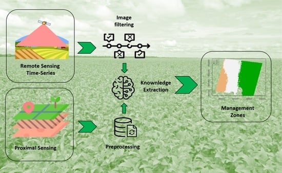
2.7. Methodology Summary

Figure 3 shows a flowchart with the steps for executing the MZ delineation regarding the four different procedures performed in each experimental plot. Attributes collected in the field (Field Attributes DS) are in vector format, while attributes related to VI (VI attributes DS) are in raster format and obtained directly from GEE platform. The VI attributes are then converted to vector format, and the field attributes are standardized to the spatial grid of them (in this case, 10 m/pixel). With all attributes standardized and in vector format, linear correlations (R) are performed between field attributes and VIs, and between the VIs themselves, to meet the requirements of the four procedures described in item 2.6. Then, the delineation of potential MZs is performed separately regarding the four subsets of attributes. Finally, for each obtained MZ map, VR is calculated regarding the historical yield of the plot. With the exception of obtaining the time series of the VIs (performed on the GEE platform), the other steps are performed by scripts developed in R language.

3. Results

This section presents the results for the proposed four procedures using different datasets to generate potential MZ maps by X-means clustering analysis, as described in Section 2. Different soil attributes (clay content, ECa and potassium) were used for each plot according to their availability as provided by the farm technical team.

3.1. Procedure 1: MZs Using Field Data and Peak-Biomass VIs

Table 4 shows the results obtained by the X-means clustering algorithm using field data and VI means in the crop’s peak biomass phase of each season.
In plots A and B, the application of identical input attributes resulted in the generation of MZ maps with differing numbers of MZs (three for A and two for B) and elevated VR values. In the case of plot C, characterized by low natural variability, particularly in terms of clay content, a soil chemical attribute was incorporated into the analysis. This addition aimed to introduce an anthropic chemical variability parameter, resulting in a significantly reduced yield VR. In plot D, which exhibits the greatest slope variability among the four plots, elevation and ECa attributes demonstrated their capacity to replace the role of the attribute clay content, yielding a relatively favorable yield VR.

3.2. Procedure 2: MZs Using Well-Correlated VIs and Soil Attributes

Table 5 shows the results obtained by the X-means clustering algorithm using the soil plot attributes and VIs that are well correlated with each other, obtained from the consolidated image for each plot.
Applying this procedure, the use of VIs along with clay content resulted in minimal changes both visually and in yield VR aspects within the MZ maps of plot A. In contrast, plot B exhibited a map divided into four MZs. One of these zones maintained the characterization of a low-average-yield area, while the other three were significantly influenced by clay content variations in a region marked by low yield variability. For plot C, even with the omission of the soil potassium map, the incorporation of VIs (EVI, SAVI, CIG and TVI) highlighted an MZ potentially associated with potassium deficiency (MZ1), resulting in an augmented yield VR compared to procedure 1. Meanwhile, for plot D, the exclusion of the average yield map introduced adjustments in MZ2, expanding its boundary towards the more productive region and increasing yield VR when contrasted with the previous procedure.

3.3. Procedure 3: MZs Using VIs Replacing Field Data

Table 6 presents the results obtained from the X-means clustering algorithm, where each attribute gathered in the field was substituted with the corresponding VI possessing the highest linear correlation (R) with it. In some cases, the same VI exhibited a higher R value in correlation with multiple attributes. Consequently, the VI was incorporated only once as an input attribute for the clustering analysis.
In plots A and B, two distinct MZs were defined, delineating regions with yields both below and above the average, yielding VR values around 40%. Plot C exhibited a pattern similar to the previous procedure, yielding a comparable VR, but with the addition of one more MZ. Clustering analysis was not performed in plot D, because the VIs presented very low linear correlation (below 0.3) with respect to all field attributes available.

3.4. Procedure 4: MZs Using VIs Selected by Variable Importance Model

Table 7 shows the results obtained by the X-means clustering algorithm using VIs that were considered paramount to estimate the yield for each plot, according to statistical measures provided by random forest models. In this case, only VIs with very high %IncMSE and IncNodePurity were selected for each plot.
In this case, plot A was divided into four MZs, one of which distinctly represents the contour lines resulting from anthropic activities performed by agricultural machinery. Nonetheless, the yield VR remained notably high (close to 50%). In plot B, the MZ outcome consistently delineated two highly distinct zones, signifying a substantial advancement over the prior procedure. These distinct zones align remarkably well with the corresponding yield map. Plot C showed a satisfactory level of consistency, with two MZs exhibiting enhanced spatial distinction. However, the yield VR within these MZs remained quite low, measuring less than 1%. In contrast, in plot D, the exclusive use of VIs to delineate MZs significantly decreased the yield VR (here and in the previous procedure) in comparison with procedures 1 and 2. For a comprehensive overview, Table 8 presents the average values of the normalized yield map for each MZ configuration.
Negative values displayed in Table 7 mean yields below the entire plot average value and positive above.

4. Discussion

The results obtained through the application of various procedures aimed at delineating MZs, involving diverse attribute sets for each plot (encompassing soil parameters, topographic data, yield maps and vegetation indices), have yielded distinct insights into the spatial variability of each plot. For both plots A and B, a degree of stability is evident despite inherent variability. This stability is facilitated by the quality of the yield maps, which enable the clear identification of contiguous regions displaying varying yields across their respective areas. Notably, both plots exhibited a significant influence of clay content when utilizing procedures 1 and 2. Introducing procedure 3, which exclusively employs VIs as input attributes, yielded well-delineated MZ maps characterized by high yield VR values. The exception was procedure 4, which provided an MZ map representing anthropic actions—a common outcome when utilizing VIs. In this instance, consolidating a single image from a 4-year time series contributes to this feature, although the exclusion of pixels assigned to it could notably enhance yield VR. Upon examining the average normalized yield for each MZ in plots A and B (Table 8), substantial differences were evident across all procedures. Average yield values ranged from 20% below to 10% above the overall plot’s average yield.
The results from plot C across all evaluated procedures indicate that the MZ maps have minimal impact on reducing yield variance. This suggests that none of these procedures should be adopted. Although soil texture data was unavailable for this plot, on-site visual inspections revealed limited variation in soil color and elevation, signifying low natural spatial variability. The low yield VR values could also result from the utilization of a single, low-quality yield map. Plots spanning 200 ha or more are typically harvested using multiple harvesters, and variations in sensor calibration can introduce noise and inaccuracies in yield maps. Hence, meticulous calibration of all yield sensors becomes essential. As a result, the combination of plot C’s low spatial variability and the noisy yield map likely contributed to the low yield VR values and the minimized normalized average yield values across all MZs and evaluated procedures (ranging from −7% to +2%, as shown in Table 8). In plots like this, other factors must be investigated, such as soil fertility parameters or pest infestation problems that might be causing low yields in specific plot regions. In plot C’s particular case, a soil potassium deficiency in its central area was identified though soil fertility analysis in grip. The MZ map generated using the soil potassium map as an input attribute (Table 1) highlights this issue. Calculating MZ yield VR by incorporating the soil potassium map instead of the yield map (procedure 1), increased VR to 67% (data not shown).
Finally, for plot D, the incorporation of consolidated VIs significantly reduced yield VR in procedures 2, 3 and 4. Unlike the others, plot D possesses substantial topographical variability and is located in a region with notably distinct climate in comparison to plots A, B and C. Additionally, this plot has been utilized over the years by the farmer for experimenting with various soybean and corn cultivars in small sections. As a result, these procedures appear to hinder the establishment of consolidated VIs over extended periods. Therefore, the use of average VIs per season, like the NDVI values during winter and summer (as employed in procedure 1), appears more fitting for this plot. This observation is further supported by the variations in MZ normalized yields detailed in Table 8. In procedure 1, where field data and VIs were solely utilized for the specific season under study, the yield differences between the two MZs amounted to 40% (20% above average for MZ1 and 20% below average for MZ2). As VI data consolidated over an extended period were employed, the separation level between the MZs diminished, resulting in a mere 11% difference between them in procedure 4. Additionally, the utilization of different cultivars for the same crop, as reported for plot D, can also exert an influence on the results.

5. Conclusions

This paper presented the results of a study that utilized a management zones (MZs) methodology for soybean–corn and soybean–cotton production systems to delineate zones based on different types of soil and crop attributes. Specifically, we examined the use of vegetation indices (VIs) as a substitute for field attributes, as they are easier to collect. Leveraging the efficiency of the Google Earth Engine (GEE) platform, we harnessed its capabilities to source and consolidate large-scale VI data.
While field data remain crucial for accurate MZ delineation, our findings and ensuing discussion highlight that proficient MZ maps can indeed be generated solely by relying on vegetation indices. Nevertheless, possessing prior knowledge of field experiments is imperative, as it directly influences the stability of VIs across the entire time series. In this context, we filtered the time series of area-specific images based solely on the presence or absence of clouds. Notably, this methodology does not require a balanced count per season due to the higher cloud incidence in summer compared to winter. Consequently, a greater number of images depicting cotton (plots A, B and C), and corn (plot D) cultivation were available compared to soybean. Another relevant issue is effectiveness of the VIs used, which are better suited for representing crop variability than soil variability.
Upon analyzing the results across all four plots, it becomes evident that VIs can effectively function as exclusive input attributes for MZ delineation in scenarios lacking significant variations in soil texture and external factors that may introduce crop variability, such as interventions involving variable rates. For upcoming works, meticulous attention should be given to the methodology used for filtering time series images. This is crucial to ensure a balanced distribution of images for each crop. Furthermore, a priority should be placed on exploring VIs that better capture soil variability, serving as substitutes for attributes like soil electrical conductivity and clay content. This endeavor involves identifying temporal windows during which the soil is exposed to enhance the efficacy of filtering time series of images.
Another aspect that requires attention is the stability of MZs once they are defined. In scenarios where MZ maps guide interventions involving variable rates, adhering to the established limits is a common practice. Thus, vegetation index maps at future dates might exhibit anthropic variability, potentially making their use impractical when adjustments to MZ delineation are needed. In such cases, alternatives like proximal sensing to assess soil and crop variability should be considered.

Author Contributions

Conceptualization, E.A.S., J.d.M.N., R.Y.I., C.M.P.V., J.C.F.d.S., I.d.O.N.L., L.A.d.C.J., L.R.Q. and L.M.R.; methodology, E.A.S., I.d.O.N.L., C.M.P.V. and J.C.F.d.S.; software, E.A.S. and L.R.Q.; validation, J.C.F.d.S. and S.d.C.; formal analysis, E.A.S., C.M.P.V., I.d.O.N.L. and J.C.F.d.S.; investigation, E.A.S., C.M.P.V., I.d.O.N.L. and L.R.Q.; resources, J.d.M.N. and R.Y.I.; data curation, E.A.S. and L.R.Q.; writing—original draft preparation, E.A.S.; writing—review and editing, E.A.S., I.d.O.N.L., J.d.M.N., C.M.P.V., J.C.F.d.S., M.X.S. and L.V.; visualization, E.A.S., J.d.M.N. and I.d.O.N.L.; supervision, E.A.S., J.d.M.N. and I.d.O.N.L.; project administration, J.d.M.N.; funding acquisition, J.d.M.N., R.Y.I. All authors have read and agreed to the published version of the manuscript.

Funding

This research was funded by the project Embrapa-Bosch-FAI, SEG: 10.22.00.001.00.00.

Data Availability Statement

To verify the possibility of using the data and scripts used in this paper, please contact the corresponding author.

Acknowledgments

The authors would like to thank the Amaggi Group and Integrada Cooperativa Agroindustrial for providing datasets for experimental soybean, corn and cotton plots.

Conflicts of Interest

The authors declare no conflict of interest.

References

  1. Moral, F.J.; Terrón, J.M.; Da Silva, J.M. Delineation of management zones using mobile measurements of soil apparent electrical conductivity and multivariate geostatistical techniques. Soil Tillage Res. 2010, 106, 335–343. [Google Scholar] [CrossRef]
  2. Damian, J.M.; Pias, O.H.D.C.; Cherubin, M.R.; Fonseca, A.Z.D.; Fornari, E.Z.; Santi, A.L. Applying the NDVI from satellite images in delimiting management zones for annual crops. Sci. Agric. 2019, 77, e20180055. [Google Scholar] [CrossRef]
  3. Ali, A.; Rondelli, V.; Martelli, R.; Falsone, G.; Lupia, F.; Barbanti, L. Management zones delineation through clustering techniques based on soils traits, NDVI data, and multiple year crop yields. Agriculture 2022, 12, 231. [Google Scholar] [CrossRef]
  4. Adiele, J.G.; Schut, A.G.; Van Den Beuken, R.P.M.; Ezui, K.S.; Pypers, P.; Ano, A.O.; Giller, K.E. Towards closing cassava yield gap in West Africa: Agronomic efficiency and storage root yield responses to NPK fertilizers. Field Crops Res. 2020, 253, 107820. [Google Scholar] [CrossRef]
  5. Moura, S.S.; Franca, L.T.; Pereira, V.S.; Teodoro, P.E.; Baio, F.H. Seeding rate in soybean according to the soil apparent electrical conductivity. An. Acad. Bras. Ciências 2020, 92, 107820. [Google Scholar] [CrossRef]
  6. García-Martínez, H.; Flores-Magdaleno, H.; Ascencio-Hernández, R.; Khalil-Gardezi, A.; Tijerina-Chávez, L.; Mancilla-Villa, O.R.; Vázquez-Peña, M.A. Corn grain yield estimation from vegetation indices, canopy cover, plant density, and a neural network using multispectral and RGB images acquired with unmanned aerial vehicles. Agriculture 2020, 10, 277. [Google Scholar] [CrossRef]
  7. Vasconcelos, J.C.S.; Speranza, E.A.; Antunes, J.F.G.; Barbosa, L.A.F.; Christofoletti, D.; Severino, F.J.; de Almeida Cançado, G.M. Development and Validation of a Model Based on Vegetation Indices for the Prediction of Sugarcane Yield. AgriEngineering 2023, 5, 698–719. [Google Scholar] [CrossRef]
  8. Gavioli, A.; de Souza, E.G.; Bazzi, C.L.; Schenatto, K.; Betzek, N.M. Identification of management zones in precision agriculture: An evaluation of alternative cluster analysis methods. Biosyst. Eng. 2019, 181, 86–102. [Google Scholar] [CrossRef]
  9. Bottega, E.L.; de Queiroz, D.M.; de Assis de Carvalho Pinto, F.; de Souza, C.M.A.; Valente, D.S.M. Precision agriculture applied to soybean: Part I-Delineation of management zones. Aust. J. Crop Sci. 2017, 11, 573–579. [Google Scholar] [CrossRef]
  10. Santos, R.T.; Saraiva, A.M. A reference process for management zones delineation in precision agriculture. IEEE Lat. Am. Trans. 2015, 13, 727–738. [Google Scholar] [CrossRef]
  11. Reyes, J.; Wendroth, O.; Matocha, C.; Zhu, J. Delineating site-specific management zones and evaluating soil water temporal dynamics in a farmer’s field in Kentucky. Vadose Zone J. 2019, 18, 1–19. [Google Scholar] [CrossRef]
  12. Georgi, C.; Spengler, D.; Itzerott, S.; Kleinschmit, B. Automatic delineation algorithm for site-specific management zones based on satellite remote sensing data. Precis. Agric. 2018, 19, 684–707. [Google Scholar] [CrossRef]
  13. Leo, S.; Migliorati, M.A.; Nguyen, T.H.; Grace, P.R. Combining remote sensing-derived management zones and an auto-aclibrated crop simulation model to determine optimal nitrogen fertilizer rates. Agric. Syst. 2023, 205, 103559. [Google Scholar] [CrossRef]
  14. Maia, F.C.O.; Bufon, V.B.; Leão, T.P. Vegetation indices as a Tool for Mapping Sugarcane Managemenz Zones. Precis. Agric. 2023, 24, 213–234. [Google Scholar] [CrossRef]
  15. Huete, A.; Didan, K.; Miura, T.; Rodriguez, E.P.; Gao, X.; Ferreira, L.G. Overview of the radiometric and biophysical performance of the MODIS vegetation indices. Remote Sens. Environ. 2002, 83, 195–213. [Google Scholar] [CrossRef]
  16. Rouse, J.W.; Haas, R.H.; Schell, J.A.; Deering, D.W. Monitoring vegetation systems in the Great Plains with ERTS. NASA Spec. Publ. 1974, 351, 309. [Google Scholar]
  17. Rahul, T.; Kumar, N.A.; Biswaranjan, D.; Mohammad, S.; Banwari, L.; Priyanka, G.; Kumar, S.A. Assessing soil spatial variability and delineating site-specific management zones for a coastal saline land in eastern India. Arch. Agron. Soil Sci. 2019, 65, 1775–1787. [Google Scholar] [CrossRef]
  18. Pearson, R.L.; Miller, L.D. Remote mapping of standing crop biomass for estimation of the productivity of the shortgrass prairie. Remote Sens. Environ. 1972, VIII, 1355. [Google Scholar]
  19. Merzlyak, M.N.; Gitelson, A.A.; Chivkunova, O.B.; Rakitin, V.Y. Non-destructive optical detection of pigment changes during leaf senescence and fruit ripening. Physiol. Plant. 1999, 106, 135–141. [Google Scholar] [CrossRef]
  20. Gitelson, A.A.; Kaufman, Y.J.; Merzlyak, M.N. Use of a green channel in remote sensing of global vegetation from EOS-MODIS. Remote Sens. Environ. 1996, 58, 289–298. [Google Scholar] [CrossRef]
  21. Broge, N.H.; Leblanc, E. Comparing prediction power and stability of broadband and hyperspectral vegetation indices for estimation of green leaf area index and canopy chlorophyll density. Remote Sens. Environ. 2001, 76, 156–172. [Google Scholar] [CrossRef]
  22. Vincini, M.; Frazzi, E.R.M.E.S.; D’Alessio, P.A.O.L.O. A broad-band leaf chlorophyll vegetation index at the canopy scale. Precis. Agric. 2008, 9, 303–319. [Google Scholar] [CrossRef]
  23. Gitelson, A.A.; Gritz, Y.; Merzlyak, M.N. Relationships between leaf chlorophyll content and spectral reflectance and algorithms for non-destructive chlorophyll assessment in higher plant leaves. J. Plant Physiol. 2003, 160, 271–282. [Google Scholar] [CrossRef]
  24. Jordan, C.F. Derivation of leaf-area index from quality of light on the forest floor. Ecology 1969, 50, 663–666. [Google Scholar] [CrossRef]
  25. Gitelson, A.; Merzlyak, M.N. Spectral reflectance changes associated with autumn senescence of Aesculus hippocastanum L. and Acer platanoides L. leaves. Spectral features and relation to chlorophyll estimation. J. Plant Physiol. 1994, 143, 286–292. [Google Scholar] [CrossRef]
  26. Huete, A.R. A soil-adjusted vegetation index (SAVI). Remote Sens. Environ. 1988, 25, 295–309. [Google Scholar] [CrossRef]
  27. Pelleg, D.; Moore, A.W. X-means: Extending k-means with efficient estimation of the number of clusters. ICML 2000, 1, 727–734. [Google Scholar]
  28. Maldaner, L.F.; de Paula Corrêdo, L.; Canata, T.F.; Molin, J.P. Predicting the sugarcane yield in real-time by harvester engine parameters and machine learning approaches. Comput. Electron. Agric. 2021, 181, 105945. [Google Scholar] [CrossRef]
  29. Dobermann, A.; Ping, J.L.; Adamchuk, V.I.; Simbahan, G.C.; Ferguson, R.B. Classification of crop yield variability in irrigated production fields. Agron. J. 2003, 95, 1105–1120. [Google Scholar] [CrossRef]
  30. Breiman, L. Random forests. Mach. Learn. 2001, 45, 5–32. [Google Scholar] [CrossRef]
Figure 1. Location map of the experimental plots.
Agriengineering 05 00092 g001
Figure 2. Images of experimental plots used in this work, considering the phenological stages of flower buds for cotton (a) and bolting for corn (b).
Agriengineering 05 00092 g002
Figure 3. Steps related to data collection and dataset generation (DS), data cleaning, standardization of spatial grids, MZ delineation and identification of VR for each MZ map presented for each experimental plot.
Agriengineering 05 00092 g003
Table 1. Attributes collected with proximal sensing and soil sampling for plots A, B, C and D.
Plot A
AttributeSource *Samples/haSpatial Int. **Mean ***SD ****
Clay (%)Soil Sampling1 Kriging47.618.7
Elevation (m)Harvest GPS785 IDW555.59.6
Cotton Yield-2019 (ton/ha) Harvest Monitor785IDW3.940.80
Cotton Yield-2020 (ton/ha)Harvest Monitor595IDW4.230.70
Soybean Yield-2021 (ton/ha)Harvest Monitor20IDW3.760.32
Soybean Yield-2022 (ton/ha)Harvest Monitor28IDW0.970.25
Plot B
AttributeSource *Samples/haSpatial Int. **Mean ***SD ****
Clay (%)Soil Sampling1 Kriging39.511.9
Elevation (m)Harvest GPS762 IDW558.96.9
Cotton Yield-2019 (ton/ha) Harvest Monitor762IDW4.620.91
Cotton Yield-2020 (ton/ha)Harvest Monitor714IDW5.511.57
Soybean Yield-2021(ton/ha)Harvest Monitor14IDW3.380.79
Soybean Yield-2022 (ton/ha)Harvest Monitor34IDW3.051.12
Plot C
AttributeSource *Samples/haSpatial Int. **Mean ***SD ****
Clay (%)Soil Sampling5Kriging45.91.30
Potassium (x)Soil Sampling5Kriging0.140.03
Cotton Yield-2022 (ton/ha)Harvest Monitor530IDW6.981.91
Plot D
AttributeSource *Samples/haSpatial Int. **Mean ***SD ****
ECa (0–50 cm)SoilXplorer Sensor326Kriging61.59.49
Soybean Yield (2022) (ton/ha)Harvest Monitor1265Kriging4.00.43
Corn Yield (2022) (ton/ha)Harvest Monitor1265Kriging7.61.15
Elevation (m)GPS Combine Harvest Monitor1265Kriging63216
* Source: source sensor or process used for data acquisition. ** Spatial Int.: interpolation algorithm used to standardize the spatial grid of the attribute (IDW: inverse distance weighting). *** Mean: mean of the attribute after spatial interpolation. **** SD: standard deviation of the attribute after spatial interpolation.
Table 2. VIs collected from GEE.
AcronymNameFormula *Reference
NDVINormalized Difference
Vegetation Index
(NIR − R)/(NIR+R)[16]
RVIRatio Vegetation IndexNIR/R[18]
PSRIPlant Senescence Reflectance Index(R − G)/RE[19]
GNDVIGreen Normalized
Difference Vegetation
Index
(NIR − G)/(NIR+G)[20]
TVITriangular Vegetation Index0.5 × (120 × (NIR − G) − 200 × (R − G))[21]
CVIChlorophyll Vegetation Index(NIR × R)/(G2)[22]
CIGChlorophyll Index—Green(NIR/G) − 1[23]
CIREChlorophyll Index—Red Edge(NIR/RE) − 1[23]
DVIDifference Vegetation
Index
NIR-RE[24]
NDRENormalized Difference Red Edge Index(NIR-RE)/(NIR+RE)[25]
EVIEnhanced Vegetation
Index
2.5 × (NIR − R)/(NIR+6 × R − 7.5 × B+1)[15]
SAVISoil-Adjusted Vegetation Index(NIR − R)/(NIR+R+0.428) × (1.428)[26]
* Formula acronyms: NIR (near infrared band); R (red band); RE (red edge band); G (green band); B (blue band).
Table 3. Linear correlation (R) average of a specific VI with the other VIs from the consolidated image of each experimental plot.
VIPlot APlot BPlot CPlot D
NDVI0.5530.5850.4510.469
RVI0.5260.1490.4250.346
PSRI0.2940.1960.4380.030
GNDVI0.6400.6160.5180.418
TVI0.6590.6410.5330.527
CVI0.6590.641−0.1250.527
CIG0.6600.6370.5330.528
CIRE0.3020.2250.3130.231
DVI0.3020.2550.3130.231
NDRE0.3180.3530.0300.053
EVI0.6680.6440.5210.525
SAVI0.5870.6110.5340.485
Table 4. MZs obtained from clustering analysis using field data and VI means in the crop’s peak-biomass phase (procedure 1). The X-axes and Y-axes of each map display, respectively, longitude and latitude coordinates in meters, considering specific reference systems for each plot (UTM Zone 21S for plots A and B, UTM Zone 22S for plots C and D).
PlotAttributesMZ Map* Av. Yield MapVR (%)
AClay
* Av. Yield
* Av. EVI
Agriengineering 05 00092 i001Agriengineering 05 00092 i00270.1
BClay
* Av. Yield
* Av. EVI
Agriengineering 05 00092 i003Agriengineering 05 00092 i00461.5
CClay
Potassium
*Av. Yield
EVI
Agriengineering 05 00092 i005Agriengineering 05 00092 i0060.1
DECa
Elevation
*Av. Yield
NDVI-Winter
NDVI-Summer
Agriengineering 05 00092 i007Agriengineering 05 00092 i00835.2
* Av. = Average.
Table 5. MZs obtained from clustering using soil field attributes and well-correlated VIs that are well correlated with each other (procedure 2). The X-axes and Y-axes of each map display, respectively, longitude and latitude coordinates in meters, considering specific reference systems for each plot (UTM Zone 21S for plots A and B, UTM Zone 22S for plots C and D).
PlotAttributesMZ Map* Av. Yield MapVR (%)
AClay
EVI
CVI
Agriengineering 05 00092 i009Agriengineering 05 00092 i01064.0
BClay
EVI
CVI
Agriengineering 05 00092 i011Agriengineering 05 00092 i01250.7
CClay
EVI
SAVI
CIG
TVI
Agriengineering 05 00092 i013Agriengineering 05 00092 i0141.3
DECa
CVI
EVI
CIG
TVI
Agriengineering 05 00092 i015Agriengineering 05 00092 i01615.4
* Av. = Average.
Table 6. MZs obtained using VIs replacing field data in input dataset (procedure 3). The X-axes and Y-axes of each map display, respectively, longitude and latitude coordinates in meters, considering specific reference systems for each plot (UTM Zone 21S for plots A and B, UTM Zone 22S for plot C).
PlotAttributesMZ Map* Av. Yield MapVR (%)
AGNDVIAgriengineering 05 00092 i017Agriengineering 05 00092 i01840.3
BGNDVI
CIG
Agriengineering 05 00092 i019Agriengineering 05 00092 i02041.6
CTVI
EVI
SAVI
CIG
Agriengineering 05 00092 i021Agriengineering 05 00092 i0221.3
* Av. = Average.
Table 7. MZs using VIs selected by variable importance model (procedure 4). The X-axes and Y-axes of each map display, respectively, longitude and latitude coordinates in meters, considering specific reference systems for each plot (UTM Zone 21S for plots A and B, UTM Zone 22S for plots C and D).
PlotAttributesMZ Map* Av. Yield MapVR (%)
ASAVI
PSRI
NDRE
GNDVI
Agriengineering 05 00092 i023Agriengineering 05 00092 i02447.9
BPSRI
NDRE
GNDVI
Agriengineering 05 00092 i025Agriengineering 05 00092 i02642.3
CPSRI
GNDVI
SAVI
Agriengineering 05 00092 i027Agriengineering 05 00092 i0280.84
DPSRI
SAVI
Agriengineering 05 00092 i029Agriengineering 05 00092 i0304.0
* Av. = Average.
Table 8. Average normalized crop yield values (normalized between −1 and 1) for each MZ delineated by the four dataset input procedures.
Plot APlot BPlot CPlot D
ProcedureMZ1MZ2MZ3MZ4MZ1MZ2MZ3MZ4MZ1MZ2MZ3MZ4MZ1MZ2
10−0.20.1-−0.20.0--−0.0080.003--0.2−0.2
20−0.20.1-0.0−0.20.10.00.020.0−0.04 0.2−01
3−0.20--0.0−0.2--0.00.01−0.02−0.07--
4−0.1−0.20.00.10.0−0.2--0.0−0.03--0.05−0.06
Disclaimer/Publisher’s Note: The statements, opinions and data contained in all publications are solely those of the individual author(s) and contributor(s) and not of MDPI and/or the editor(s). MDPI and/or the editor(s) disclaim responsibility for any injury to people or property resulting from any ideas, methods, instructions or products referred to in the content.

