Photodetector Spectral Response Estimation Using Black Body Radiation


1
MBDA Italia S.p.A. Via Monte Flavio, 45-00131 Roma, Italy
2
University of Cassino and Southerm Lazio, Via G. Di Biasio, 43 Cassino (FR), Italy
*
Author to whom correspondence should be addressed.
Physics 2019, 1(3), 360-374; https://0-doi-org.brum.beds.ac.uk/10.3390/physics1030026
Submission received: 3 July 2019
/
Revised: 5 November 2019
/
Accepted: 6 November 2019
/
Published: 19 November 2019
(This article belongs to the Section Applied Physics)
Abstract
:We propose a method for the estimation of the spectral response of a photodetector, using only the variation of the temperature of a black body source without the need of an expensive monochromator or a circular filter. The proposed method is suitable especially for infrared detectors in which the cut-off wavelength and the responsivity vs. wavelength is not exactly known. The method provides a rough estimation of the spectral response solving a Fredholm integral equation of the first kind. The precision of this technique depends on the temperatures at which the detector output is measured. Some examples are given for illustration.
1. Introduction
Infrared photodetectors are currently used in many applications; in civil and military applications [1], in particular for surveillance [2,3], target detection and tracking for missile systems and night vision in battlefields [4]. Other applications concern satellite imaging and astronomical observations. One of the most promising fields of application is the passive detection of infrared radiation coming from objects in a given field of view. In order to design an infrared passive system it is mandatory to know the parameters characterizing the detector [5]. For the staring detectors the noise-equivalent temperature difference (NETD) is very important because it gives information about the sensitivity of the 2D array. Another important parameter is the responsivity. Responsivity can be defined as the ratio between the electrical signal of the detector and the incident optical power. The black body responsivity is defined as the ratio of the signal (voltage or current) and the total power emitted by a black body [6]:
where V is the output voltage of the detector, is the Stefan-Boltzmann constant and T is the absolute temperature (in K).
Unfortunately, in the case of real detectors, only a little amount of this power is ‘seen’ by the detector and in particular in the case of photonic detectors, only the power between zero wavelength and cut-off wavelength creates electron–hole pairs. So the real responsivity [6] is the ratio between the electrical signal and the power, which can also be expressed:
where is the wavelength in m, represents the Planck radiation law:
and is the spectral response of the detector [6]. Here and are Kirchoff constants. When the detector is made using a single element semiconductor like silicon or germanium, the cut-off wavelength and the spectral are known with a little error [7]. Moreover, in the case of two element alloys like the cut-off wavelength can be considered known and so the . The case of , for example, is quite different because the cut-off wavelength and the spectral response function could be unknown if we do not know the molar ratio of and . Taking into account this problem, it is very important to measure or to estimate the spectral response function [2]. The best method is to use a monochromator [8,9] in order to measure it exactly, but this is a very expensive device that may not be always available in the laboratory. For a rough estimate of this quantity we propose a method based only on the variation of the temperature of a calibrated black body.
2. The Method
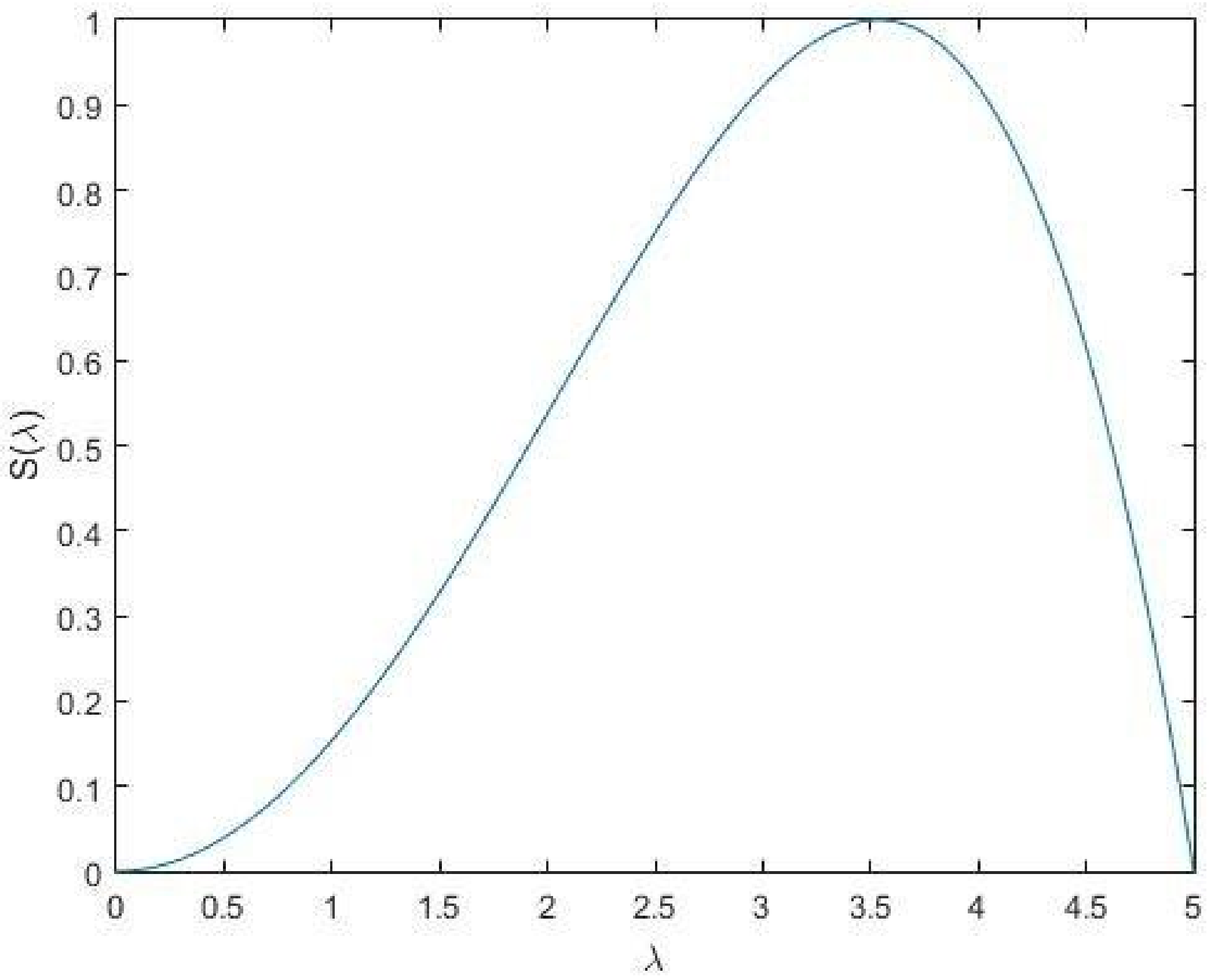
The study should be conducted considering the black body as a radiating source. The black-body radiation power is given by Equation (3) where the Kirchoff constants are = 37,418 and = 14,388. The radial spectral density curve, calculated, for example, at 500 K, is reported in Figure 1. Integrating the Planck function between and , it is possible to calculate the incident power on a photodetector as:
where r is the radius of the black-body aperture in m, is the radius of the receiver’s optical aperture in m, L is the distance between the black body and the photodetector in cm, is computed from the Stefan-Boltzman equation:
Given the incident optical power with the photodetector it is possible to compute the black-body responsivity as the ratio between the photodetector output voltage (or current) and the optical incident power [10,11,12]:
Equation (6) does not take into account the spectral response of the photodetector that increases until the cut-off frequency, where it falls to zero. In order to know the exact amount of optical power seen by the detector it is very important to know the spectral response of the detector. In general, this function can be obtained using optical devices like filters or monochromators [13]. The peak responsivity, , which is a function of the spectral response of the photodetector, is:
where is the integral of Equation (2). From Equation (2) it is possible to compute the photodetector peak responsivity taking into account the function . For this purpose, considering the expression:
and defining as:
the photodetector output voltage is proportional to the function by the constant . Observing Equation (2), one notes that the upper integration limit coincides with the sensor’s cut-off wavelength as soon as there is no response above the cut-off frequency. So, the expression for can be written as:
The equation is tied to the temperature [11] so that, in general, there will be an integral function for each temperature :
3. Generality of the Problem
Starting from the Fredholm integral of the first kind [14], it is necessary to find out a method for estimation of the unknown function :
The generic function can be expressed as a series of functions [14] where are the basis functions:
The integral will be:
Now it is possible to use the matrix formalism in order to obtain:
where:
So, in a compact representation, the vector is the product of the matrix and the coefficient vector a:
Once all the coefficients have been computed, it is possible to reconstruct the unknown function . The robustness of the estimation method against the measurement error is discussed in Appendix A.
4. Estimation with Basis Function
In this paper, some basis functions have been identified for the approximation of the spectral response of photodetectors.
- Laguerre polynomials. The polynomials are defined as [14]:In this case one gets:The integral expression for the computation of the matrix elements reads:
- Hermite polynomials. These polynomials are defined as [14]:The integral expression for the computation of the matrix elements is:
- Sinc function. This function is defined as [14]:The resolution of the Fredholm equation requires some manipulations with the function. In a finite interval it can be considered a basis function,where:and h is the sample step. Then, the function, integrated in order to calculate the elements of the matrix , is:Considering the function , from its symmetry, the sum runs from to N:
5. Results
The analysis was carried out using Matlab®. The first step was to simulate a photodetector output voltage measurement using a known spectral response. This allows us to have a vector of elements that is just the output voltage to the photodetector. The function that best approximates the normalized spectral response of a photonic detector (, [18,19]) operating in the first atmospheric window is [20]:
The performance of this function is shown in Figure 2. The analysis was carried out in the band [0–5] m. From the figure we notice that at the extremes of the band the spectral response is canceled. Moreover, if when using this function for a higher wavelength it has negative values, there are at that time no problems because it is only used in the right band. Subsequently, we move to the calculation of the spectral response using the tension vector found by the previous simulation; this type of approach is permitted, as the actual voltage measurements are known. For the calculation of S, we proceeded in the way discussed in Section 3 by evaluating the performance of the basis functions. Basically speaking we have a vector of tensions varying the black-body temperature, a metric obtained by Equation (16) and an unknown vector of coefficients of the series in Equation (14) in which now .
5.1. Power Series Approximation
In this case we have selected a power series for the basic function. The procedure described in Section 2 allows us to evaluate the performance in terms of system error. The error was calculated computing the difference between the desired function and the reconstructed function. Other factors to be considered are the inversion of the matrix J and the number of points to be used in the reconstruction. The analyses were conducted at T = [500–700] K, = [0–5] m, L = 10 cm, = 0.01 cm, r = 0.1 cm, V/W. The parameter that was varied was the number of points N, for values up to . One can rebuild the spectral response function S very accurately, but with an increase in the number of points, Matlab® does not guarantee with enough precision with the inverse matrix computation. In the case of , we can see how the function is estimated. Looking at Figure 3 the curves are superimposed in the seven points where the function is estimated with the power series. It is possible to estimate the function with a maximum error of , the error is calculated with the difference between the known function and the reconstructed one with the basic function. Because of the mathematical features of the power series, as soon as the number of points increase, the basis function cannot be used to accurately describe the unknown response function. Moreover, one faces difficulties with the inverse matrix of J as its determinant is of the order of . Obviously, the error increases proportionally to the number of points. For example, in the case of there is a difference between the reconstructed and the known function of , which is very high considering that the maximum of the function is 1 (Figure 3).
5.2. Laguerre Polynomials Approximation
In this case the basis functions are Laguerre polynomials. From Equation (21) one can see that even in this case it is possible to face difficulties similar to those seen with the power series approximation. The simulation parameters were the same as before and we assessed how far we could increase the degree of the Laguerre polynomial. From the analyses carried out in such conditions, we can push the order of polynomials up to with an error of (Figure 4). Moving to it is no longer possible to reconstruct the function, and the inversion of matrix J is not accurate.
5.3. Hermite Polynomials Approximation
In this case the number of points is taken even smaller in order not to face difficulties with the reconstruction and with the inversion of the matrix. In fact a number of points less than were used. Let us analyse the case of . The ideal curve and the real curve are superimposed, so the reconstruction was done correctly, considering also that the error is . By raising the number of points and then the degree of polynomials, we have a good reconstruction of the function, but one faces difficulties with the inverse of the J matrix for (Figure 5).
5.4. Approximation with Sinc Functions
For the estimation of the spectral response with the Sinc function, we need to make additional considerations since the basis function of Equation (27) seen in the previous section gets difficulties at the extremes of the range. At the m the logarithm tends to minus infinity and therefore this limits the approach. Therefore, we restricted the band considering a lower wavelength of 1 m. As far as the upper peak is concerned, in the cut-off frequency analysis we have the deletion of the denominator of the fraction in the logarithm Equation (4) and therefore not a suitable value for the analysis. To this purpose, we shifted a small amount with respect to the cut-off frequency in order to avoid the zero in the denominator of the logarithm. In the case of Sinc, we have seen that the sum of the spectral response reconstruction goes from to N, so the analysis is made on points. Let us evaluate the case with (Figure 6). It can be noted that the function is reconstructed fairly faithfully up to the cut-off frequency where we find a deviation between the reconstructed and ideal spectral response. In this case, however, the inversion of matrix J is not accurate. We propose the analysis with where we have a corrected inverse matrix but loose the maximum of the function (Figure 6).
6. Conclusions
The proposed method is useful whenever the spectral responsive function of a detector is unknown. We proposed several basis functions to solve the Fredholm integral equation obtained varying the black-body temperature. With this method we can get a rough approximation of the spectral response and so of the cut-off wavelength. The roughness of the spectral response estimation depends on the number of measurements carried out. We applied this method using a simulated but realistic spectral response and we showed that it is one that can rebuild the function with a good level of approximation using only five or six measurements. It is worth noticing that the requirement time of the measurements process is of about 20–30 min overall.
7. Patents
EU Patent EP2947435(A1): Method for Estimating the Spectral Response of An Infrared Photodetector
US Patent US20150330837: Method for Estimating the Spectral Response of An Infrared Photodetector
IT Patent 0001423853: Metodo per la stima della risposta spettrale di un fotorilevatore ad infrarossi
Author Contributions
Conceptualization and formal analysis, R.M.L. and M.R.; software and writing—original draft, A.D.P.
Funding
This research received no external funding.
Conflicts of Interest
The authors declare no conflict of interest.
Abbreviations
The following abbreviations are used in this manuscript:
| NETD | Noise equivalent temperature difference |
Appendix A. Measurement Error Analysis
The method for estimating the spectral response of electro-optical sensors is robust compared to measurement errors. The errors can be both related to the accuracy of the tools used for voltage reading and the error on measuring the temperature of the black body. The errors related to the diameter of the opening of the black body and the diameter of the optics turn out to be negligible. The analysis of the errors introduced is reported below, and performed as follows.
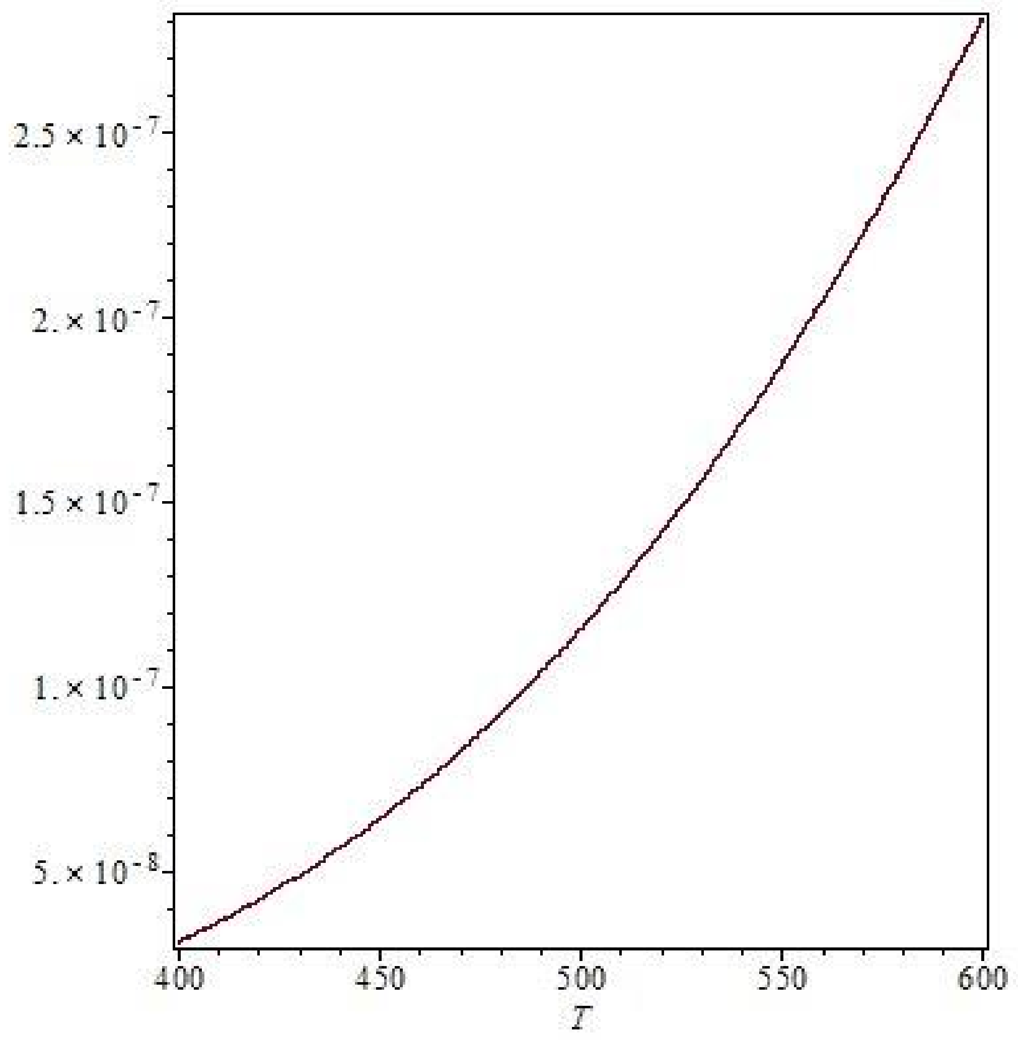
- Addressing the integral (Equation (2)) one can analyze the variation with respect to the temperature of the black body:considering a black body temperature of between 400 and 600 K; the derivative of the previous one is less than 1. It follows that using a perfectly calibrated black body, the error in the measurement of the temperature does not affect the integral (Figure A1).Figure A1. at according to the temperature of black-body.
![Physics 01 00026 g0a1]()
- With regard to the error introduced in the voltage, one can write the equation (Equation (18)) in which the vector is given by the voltage measurements V:We assume that:The a coefficients can be written as:Resolving Equation (A4) with respect to one obtains:Then a small variation of V results in a small variation of a.

In what follows, the spectral response function is reconstructed by adding to the voltage a error of with respect to the nominal value of the measured voltage (Equation (A2)), V. This takes into account the measurement error that can be committed in the acquisition of the sensor output. The analysis is carried out for the same cases as discussed in Section 5.
Appendix A.1. Power Series Approximation
In the case of power series approximation with , the function is reconstructed in the same way as without error (Figure A2), and the difference between the reconstructed spectral response with the measurements without error (V) and the reconstruction made with the measurements containing the error () is reported in Figure A3.
Figure A2.
Reconstruction of the spectral response function with power series compared to the voltage error case.
Figure A2.
Reconstruction of the spectral response function with power series compared to the voltage error case.

Figure A3.
The difference between the spectral response with error in the voltage and without it using the power series approximation.
Figure A3.
The difference between the spectral response with error in the voltage and without it using the power series approximation.

Appendix A.2. Laguerre Polynomials Approximation
In the estimation of the spectral response with the Laguerre polynomials (), the function is reconstructed similarly to as the no-error reconstruction (Figure A4), and the difference between the reconstructed spectral response with the measurements without error (V) and the reconstruction made with the measurements containing the error () is reported in Figure A5.
Figure A4.
Reconstruction of the spectral response function with Laguerre polynomials compared to the voltage error case.
Figure A4.
Reconstruction of the spectral response function with Laguerre polynomials compared to the voltage error case.

Figure A5.
The difference between the spectral response with error in the voltage and without it using Laguerre polynomials.
Figure A5.
The difference between the spectral response with error in the voltage and without it using Laguerre polynomials.

Appendix A.3. Hermite Polynomials Approximation
The estimation of spectral response with the Hermite polynomials () reconstructed in the same way as in the case without error is shown in Figure A6, and the difference in the estimate between the case with a error in the voltage and the ideal case without error is represented in Figure A7.
Figure A6.
Reconstruction of the spectral response function with Hermite polynomials compared to the voltage error case.
Figure A6.
Reconstruction of the spectral response function with Hermite polynomials compared to the voltage error case.

Figure A7.
The difference between the spectral response with error in the voltage and without it using Hermite polynomials.
Figure A7.
The difference between the spectral response with error in the voltage and without it using Hermite polynomials.

Appendix A.4. Approximation with Sinc Functions
The estimation of spectral response with the Sinc functions () was reconstructed in the same way as the case without error (Figure A8), and the difference in the estimate between the case with a error on the voltage and the ideal case without error is represented in Figure A9.
Figure A8.
Reconstruction of the spectral response function with Sinc functions compared to the voltage error case.
Figure A8.
Reconstruction of the spectral response function with Sinc functions compared to the voltage error case.

Figure A9.
The difference between the spectral response with error on the voltage and without it using Sinc function approximation.
Figure A9.
The difference between the spectral response with error on the voltage and without it using Sinc function approximation.

References
- Jha, A.R. Infrared Tecnology: Applications to Electro-Optics, Photonics Devices and Sensors; John Wiley & Sons, Inc.: Hoboken, NJ, USA, 2008. [Google Scholar]
- Vincent, J.D.; Hodges, S.E.; Vampola, J.; Stegall, M.; Pierce, G. Fundamentals of Infrared and Visible Detector Operation and Testing; John Wiley & Sons, Inc.: Hoboken, NJ, USA, 2015. [Google Scholar]
- Vollemer, M.; Mollmann, K.P. Infrared Thermal Imaging: Fundamentals, Reserarch and Applications; WILEY-VCH Verlag GmbH & Co. KGaA: Weinheim, Germany, 2018. [Google Scholar]
- Richard, D.H., Jr. Infrared System Engineering; John Wiley & Sons: Hoboken, NJ, USA, 2006. [Google Scholar]
- Keyes, R.J. (Ed.) Optical and Infrared Detectors; Springer: Berlin/Heidelberg, Germany, 1980. [Google Scholar]
- Miller, J.L.; Friedman, E. Photonics Rules of Thumb: Optics, Electro-Optics, Fiber Optics, and Lasers; McGraw-Hill: New York, NY, USA, 2004. [Google Scholar]
- Ahmed, S. Physics and Engineering of Radiation Detection; Elsevier: Amsterdam, The Netherlands, 2014. [Google Scholar]
- Riazimehr, S.; Bablich, A.; Schneider, D.; Kataria, S.; Passi, V.; Yim, C.; Duesberg, G.S.; Lemme, M.C. Spectral sensitivity of graphene/silicon heterojunction photodetectors. Solid-State Electron. 2016, 115, 207–212. [Google Scholar] [CrossRef]
- Faria, L.A.; Nohra, L.F.M.; Gomes, N.A.S.; Alves, F.D.P. A high-performance test-bed dedicated for responsivity measurements of infrared photodetectors in a wide band of low temperatures. Int. J. Optoelectron. Eng. 2012, 2, 12–17. [Google Scholar] [CrossRef] [Green Version]
- Willardson, R.K.; Beer, A.C. (Eds.) Semiconductors and Semimetals, Volume 12: Infrared Detectors II; Academic Press: Cambridge, MA, USA, 1977. [Google Scholar]
- Lloyd, J.M. Thermal Imaging Systems; Springer: New York, NY, USA, 1975. [Google Scholar]
- Kingston, R.H. Detection of Optical and Infrared Radiation; Springer: Berlin/Heidelberg, Germany, 1978. [Google Scholar]
- Arrasmith, W.W. System Engineering and Analysis of Electro-Optical and Infrared Systems; CRC Press: Boca Raton, FL, USA, 2015. [Google Scholar]
- Polyanin, A.D.; Manzhirov, A.V. Handbook of Integral Equations; Chapman and Hall/CRC: Boca Raton, FL, USA, 2008. [Google Scholar]
- Wolfe, W.L. Infrared Design Examples; SPIE Press: Bellingham, WA, USA, 1999. [Google Scholar]
- Wolfe, W.L. Introduction to Infrared System Design; SPIE Press: Bellingham, WA, USA, 1996. [Google Scholar]
- Willers, C.J. Electro-Optical System Analysis and Design: A Radiometry Perspective; SPIE Press: Bellingham, WA, USA, 2013. [Google Scholar]
- Willardson, R.K.; Beer, A.C. (Eds.) Semiconductors and Semimetals, Volume 5: Infrared Detectors; Academic Press: Cambridge, MA, USA, 1970. [Google Scholar]
- Kinch, M.A. Fundamentals of Infrared Detector Materials; SPIE Press: Bellingham, WA, USA, 2007. [Google Scholar]
- Saxena, P.K. Infrared Photodetectors: Some Techiniques for Modeling and Simulation; LAP Lambert Academic Publishing: Saarbruecken, Germany, 2018. [Google Scholar]
Figure 1.
Energy density curve for T = 500 K.

Figure 2.
Theoretical spectral response used for simulations.

Figure 3.
Spectral response function reconstruction with power series.

Figure 4.
Spectral response function reconstruction with Laguerre polynomials.

Figure 5.
Spectral response function reconstruction with Hermite polynomials.

Figure 6.
Spectral response function reconstruction with “Sinc” functions.

© 2019 by the authors. Licensee MDPI, Basel, Switzerland. This article is an open access article distributed under the terms and conditions of the Creative Commons Attribution (CC BY) license (http://creativecommons.org/licenses/by/4.0/).
Share and Cite
MDPI and ACS Style
Liberati, R.M.; Del Paggio, A.; Rossi, M. Photodetector Spectral Response Estimation Using Black Body Radiation. Physics 2019, 1, 360-374. https://0-doi-org.brum.beds.ac.uk/10.3390/physics1030026
AMA Style
Liberati RM, Del Paggio A, Rossi M. Photodetector Spectral Response Estimation Using Black Body Radiation. Physics. 2019; 1(3):360-374. https://0-doi-org.brum.beds.ac.uk/10.3390/physics1030026
Chicago/Turabian StyleLiberati, Riccardo Maria, Alessio Del Paggio, and Massimiliano Rossi. 2019. "Photodetector Spectral Response Estimation Using Black Body Radiation" Physics 1, no. 3: 360-374. https://0-doi-org.brum.beds.ac.uk/10.3390/physics1030026