Article

A Full-Fledged Analytical Solution to the Quantum Harmonic Oscillator for Undergraduate Students of Science and Engineering

by
Arturo Rodríguez-Gómez
1,* and
Ana Laura Pérez-Martínez
2
1
Instituto de Física, Universidad Nacional Autónoma de México, Ciudad de México 04510, Mexico
2
Facultad de Ingeniería, DCB, Universidad Nacional Autónoma de México, Ciudad de México 04510, Mexico
*
Author to whom correspondence should be addressed.
Submission received: 11 September 2020 / Revised: 2 October 2020 / Accepted: 2 October 2020 / Published: 17 October 2020
(This article belongs to the Section Physics Education)

Abstract

:
The quantum harmonic oscillator is a fundamental piece of physics. In this paper, we present a self-contained full-fledged analytical solution to the quantum harmonic oscillator. To this end, we use an eight-step procedure that only uses standard mathematical tools available in natural science, technology, engineering and mathematics disciplines. This solution is accessible not only for physics students but also for undergraduate engineering and chemistry students. We provide interactive web-based graphs for the reader to observe the shape of the wave functions for an electron and a proton when both are subject to the same potential. Each of the eight steps in our solution procedure is treated as a separate problem in order to allow the reader to quickly consult any step without the need to review the entire article.

1. Introduction

Currently, most of the materials science graduate programs offered at various universities worldwide have a strong multi- and interdisciplinary character [1,2]. Therefore, graduates who aspire to join these programs must possess competent knowledge in mathematics, engineering, physics, and chemistry. To achieve this goal, some universities offer short preparatory courses, which allow applicants to overcome possible deficiencies inherent to their respective undergraduate curricula. In this sense, students who enroll in physics courses generally have academic backgrounds in engineering or chemistry. Such students and their teachers are the principal motivation for this work.
The quantum harmonic oscillator (QHO) is a fundamental piece of physics. Many subjects converge in the study of the QHO, among which modern physics [3,4,5,6], quantum chemistry [7], condensed matter [8], structure of matter [9], and quantum mechanics [10,11,12,13] stand out. Understanding the QHO solution provides the student with powerful tools to tackle more complex problems related to quantum physics. Furthermore, the QHO can model and explain practical phenomena, including infrared and Raman spectroscopies [14], blackbody radiation [15], stereomutation in chiral molecules [16], and entropy calculations of single molecules [17].
However, the first-time student looking for reliable sources to study the QHO on his own may be overwhelmed by the ubiquity of the topic and the great diversity in which it is addressed. The most popular books in modern physics only present the QHO wave functions without discussing its origin [3,4]. They also present disclaimers such as “the mathematical techniques involved in solving this type of differential equation are standard in mathematical physics but unfamiliar to most students at this level” [5] and “the mathematical technique for solving this equation is beyond the level of this text” [6]. On the other hand, when the student consults books on quantum mechanics [10,11,12,13,18], the balance tips to the other extreme. In those sources, one will find unfamiliar concepts that would take time to learn and apply, such as Dirac’s notation [10], or the algebraic solution method that makes use of annihilation and creation operators [11,12,13].
Although to a lesser extent, it is also possible to find introductory books on quantum physics. That bibliography presents the analytical solution of the QHO, with an approach that attempts to reconcile the prevailing scarcity in modern physics books with the “mathematical sophistication” of quantum mechanics books [18,19,20]. However, in our understanding, those books do not ultimately achieve the said goal; first, because they are intended for physics students who naturally have solid foundations in mathematics. Additionally, none of those references offer detailed explanations of the different stages that integrate the whole solution. According to our experience, those missing explanations are of great value for inexperienced students in short courses.
In this paper, we present a full-fledged analytical solution to the QHO using an eight-step solution procedure. We built this strategy over ten years of experience teaching short courses in quantum physics and structure of matter to students with backgrounds in chemistry and engineering. Our procedure is self-contained and implicitly includes detailed explanations to questions that recurrently appear during our courses. We only use standard mathematical tools available in natural science, technology, engineering and mathematics disciplines generally from the second college year. We believe this document can help the beginning reader to understand, enjoy, and take advantage of other smart and elegant ways to approach the QHO problem [21,22,23,24,25,26]. This methodology could also be useful for the first-year physics student taking introductory subjects in quantum physics or modern physics.

2. Discussion

Heretofore, the beginning physics student should have worked with potentials that are constant and discontinuous position functions. By studying the quantum harmonic oscillator (QHO), we will take a step towards to a more realistic scenario. For this case, V( x ) will be a continuous position function of the type V x = α   x 2 . The QHO can be used to describe almost any system in which a certain entity makes small vibrations with respect to an equilibrium point.
In Figure 1a, we show a one-dimensional potential that is described with a solid line. This potential has a minimum point, for which it is possible to approximate a parabolic function V( x ) represented by the dashed line.
If we set the origins of the position and energy axes to coincide at the minimum of the “realistic” potential, then we can plot our parabolic approximation, as illustrated in Figure 1b. Equation (1),
V x = C 2 x 2 ,
describes this parabola, and we will discuss the precise origin of this expression in the first section of our solution procedure
The potential of Equation (1) is a quadratic function of the type y x = a x 2 + b x + c . When the constants b and c are zero, then the parabola vertex is at the origin. Meanwhile, the constant a narrows the parabola as the value increases; in this case, constant a = C 2 .
A particle under the influence of Equation (1) potential experiences a linear restoring force equal to that observed in Hooke’s law:
F x = d V x d x = C x ,
where C can be interpreted as the spring force constant.
Before entering the solution procedure for the QHO, it is interesting and imperative to review the classical results for a particle under the influence of a restoring force. If we call the restoring force F s , then we will have the following:
F s = C x     F s = m a x     C x = m a x     a x = C m x     d 2 x d t 2 = a x     d 2 x d t 2 = C m x .
We can introduce ω 2 = C m , and then
d 2 x d t 2 = ω 2 x .
The latter is a homogeneous differential equation with constant coefficients, whose solution is of the type
x t = A cos ω t + ϕ ,
where ω is the angular frequency, and thus the frequency ν is ν = ω 2 π .
Then, when the particle moves a distance A from its equilibrium point, it will oscillate in simple harmonic motion with a frequency equal to
ν = 1 2 π C m ,
where C is the restoring force constant and m is the particle’s mass.
We should also recall that, according to classical mechanics, the particle’s total energy E, which is the sum of the kinetic (K.E.) and potential (P.E.) energies, is proportional to A 2 , and therefore E is allowed to take any value. Let us verify this through the following expressions:
K . E . = 1 2 m v 2 , x t = A cos ω t + ϕ     v t = d   x t d t = ω A sin ω t + ϕ , K . E . = 1 2 m ω 2 A 2 sin 2 ω t + ϕ     due   ω 2 = C m , K . E . = 1 2 C A 2 sin 2 ω t + ϕ , P . E . = 1 2 C x 2     1 2 C A 2 cos 2 ω t + ϕ , E = K . E . +   P . E . = 1 2 C A 2 sin 2 ω t + ϕ + cos 2 ω t + ϕ .
By using the trigonometric identity sin 2 ω t + ϕ + cos 2 ω t + ϕ = 1 , we have
E = 1 2 C A 2 .
Thus, it is clear, from a classical point of view, that a particle with simple harmonic motion can take any energy value.
On the other hand, quantum mechanics predicts that a particle bound to a certain region of finite size will have a set of discrete energy values, as in the case of a potential well. We will establish that these discrete energy predictions also appear on the quantum harmonic oscillator.
To obtain a full-fledged analytical solution for the QHO, we propose a methodology divided into eight segments. We present each section as an independent problem, very simple to solve, and explained in detail. The mathematical tools to follow the problem’s solution are available to any engineering or science student. The sum of these eight small problems constitutes the analytical solution for QHO. These sections are as follows:
  • Determination of the quadratic potential V x ;
  • Use of V x potential in the time-independent Schrödinger equation to obtain a dimensionless differential equation;
  • Manipulation of the dimensionless differential equation to determine its solution’s form at infinity;
  • Determination of the recursion relation that allows us to obtain complete solutions for the dimensionless differential equation;
  • Comparing successive power coefficients for the functions H u and e u 2 and to determine the quantization condition;
  • Writing the odd and even solutions using Hermite polynomials and writing the formulas for the energy eigenvalues;
  • Obtaining non-normalized eigenfunctions;
  • Normalization of the eigenfunctions and graph for levels 0, 1, 2, and 10.

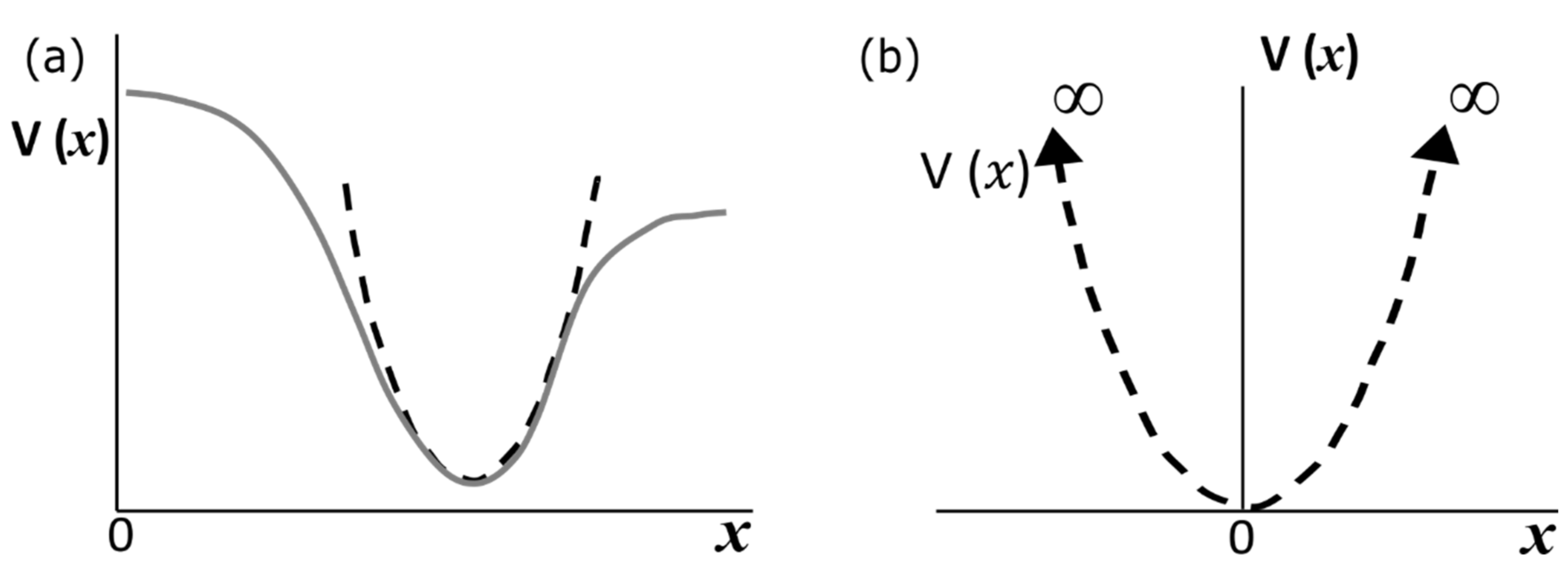
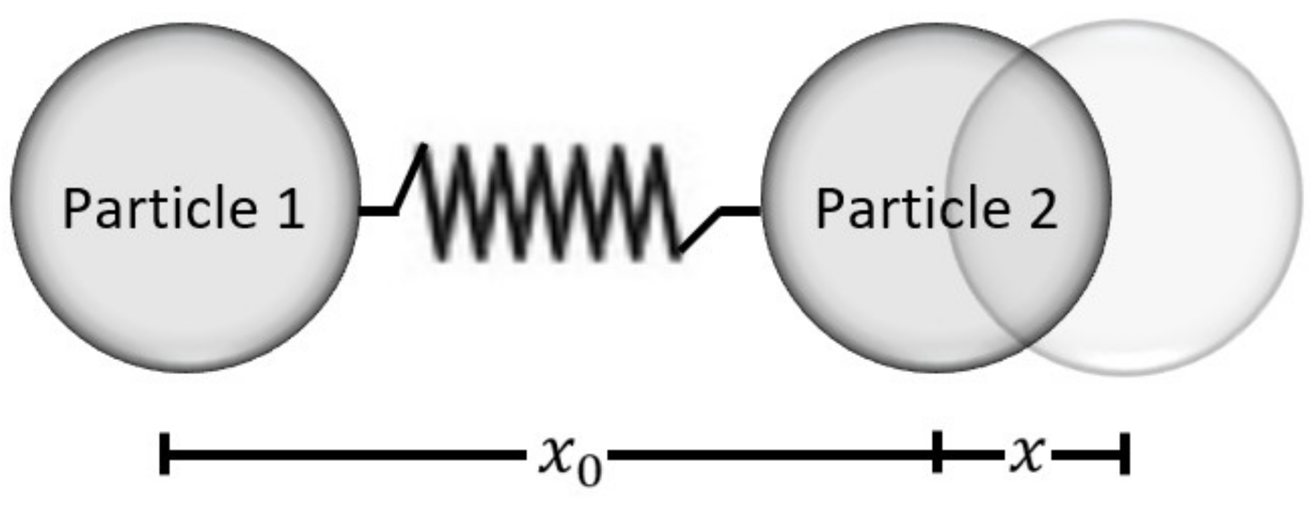
2.1. Determination of the Quadratic Potential V x

Consider the pair of particles of Figure 2. They have a simple harmonic oscillator behavior; i.e., the force between them depends on a displacing distance x that is counted from an equilibrium position x 0 .
In this case, we can express the potential function as a Taylor series. The definition for the Taylor series centered at the point a is
f x = n = 0 f n a n ! x a n .
We calculate some terms:
f x = f a 0 ! x a 0 + f a 1 ! x a 1 + f a 2 ! x a 2 +
We want our function to be centered on the equilibrium point x 0 ; therefore, a = x 0 :
f x = f x 0 0 ! x x 0 0 + f x 0 1 ! x x 0 1 + f x 0 2 ! x x 0 2 +
For the first term, we have f x 0 = const = V 0 . Meanwhile, for the second term, we have f x 0 1 ! = const = V 1 , and the third term can be expressed as f x 0 2 ! = 1 2 const = 1 2 V 2 .
Consequently, we can write our potential function as follows:
V x =   V 0 + V 1 x x 0 + 1 2 V 2 x x 0 2 +
We only keep the first three terms of the series because the value x x 0 is small for small displacements from the equilibrium position x 0 .
With the previous function in mind, one can see that at x = x 0 , we have a minimum, and in consequence, d V x d x = 0 . For the above to be true, it requires that V 1 = 0 . Additionally, we can redefine the zero-potential energy at V 0 = 0 (Figure 1b). Then, one can immediately identify that the last remaining term of the potential function V x is
1 2 V 2 x 2 .
This is the origin of the quadratic potential V x that appears in most modern and introductory quantum physics books. We only need to replace the constant V 2 with the constant C to obtain Equation (1) that we presented previously,
V x = C 2 x 2 .

2.2. Use of V x Potential in the Time-Independent Schrödinger Equation to Obtain a Dimensionless Differential Equation

Recall that the time-independent Schrödinger equation is [3].
2 2 m d 2 ψ x d x 2 + V x ψ x = E   ψ x .
Substituting the potential of Equation (1) into the time-independent Schrödinger equation, we have
2 2 m d 2 ψ d x 2 + C 2 x 2 ψ = E   ψ .
On the other hand, Equation (2) defines the classical oscillation frequency υ in terms of the force constant C and the particle’s mass m. Using that expression, we can obtain the value of C in terms of υ ,   π , and m,
ν = 1 2 π C m     ν 2 = 1 4 π 2 C m     C = ν 2 4 π 2 m .
We introduce constant C into Equation (3) to obtain,
2 2 m d 2 ψ d x 2 + ν 2 4 π 2 m 2 x 2 ψ = E   ψ     2 2 m d 2 ψ d x 2 + 2 m π 2 ν 2 x 2 ψ = E   ψ .
We rearrange the last expression as follows:
2 2 m d 2 ψ d x 2 = E   ψ 2 m π 2 ν 2 x 2 ψ     2 2 m d 2 ψ d x 2 =   ψ E 2 m π 2 ν 2 x 2     d 2 ψ d x 2 =   2 m 2 ψ E 2 m π 2 ν 2 x 2     d 2 ψ d x 2 + 2 m E 2 2 m π ν 2 x 2 ψ = 0 .
We defining α and β values as
α = 2 m π ν       and   β = 2 m E 2 .
We can write the equation as follows:
d 2 ψ d x 2 + 2 m E 2 2 m π ν 2 x 2 ψ = 0 ,
d 2 ψ d x 2 + β α 2 x 2 ψ = 0 .
Let us pause briefly to identify the units of the α and β values. To this end, remember that
E = m a s s l e n g t h 2 t i m e 2 = M L 2 T 2 ;   = m a s s l e n g t h 2 t i m e = M L 2 T ;   ν = 1 t i m e = 1 T .
Hence for α and β , we have that
α = M 1 T M L 2 T = M T M L 2 T = M T M T L 2 = L 2   and   β = M M L 2 T 2 M L 2 T 2 = M 2 L 2 T 2 M 2 L 4 T 2 = M 2 L 2 T 2 M 2 L 4 T 2 = L 2 .
In other words, Equation (5) is not yet a dimensionless equation. To make the equation dimensionless, let us propose a variable change. Due to the units of α, a good proposal for the new variable is u = α   x .
Since α = 2 m π ν and ν = 1 2 π C m , then α =   2 π m ν 1 2 . By carrying out the corresponding algebra we have
α = 2 π m 1 2 π C m 1 2     α = m 1 2 C m 1 4 = m 1 2 1 2 C 1 4 m 1 4     α = m 1 4 C 1 4 1 2     α = C m 1 4 1 2 .
Consequently, we can also write u in the following way:
u = α   x = C m 1 4 1 2 x .
Equation (5) is a differential equation where the unknown is the function ψ x . We are proposing a variable change from x to u ; as a result, ψ x will become ψ u . Since Equation (5) contains a second derivative of the ψ x function, we need to calculate the corresponding second derivative of ψ u function. We must use the well-known chain rule whenever we make a variable change in a differentiable function. Let us use a very simple example to remember Leibniz’s notation for the chain rule.
d d x sin x 2 , u = x 2 , d f d x = d f d u d u d x ; d d u sin u d d x x 2 = cos u 2 x = 2 x cos x 2 .
Next, we will use the chain rule to get the first and second derivatives of the ψ(u) function:
d ψ x d x = d ψ u d u d u d x } We can, and we must derive this term with respect to x .
Since ψ x is the unknown of Equation (5).
d ψ u d u should remain expressed as a derivative
d u d x = d d x α   x = α .
Therefore,
d ψ x d x = d ψ u d u d u d x = α d ψ u d u .
For the second derivative case, the chain rule includes a product rule, and it is expressed as follows:
d 2 ψ x d x 2 = d 2 ψ u d u 2 d u d x 2 + d ψ u d u d 2 u d x 2 = α d 2 ψ u d u 2 .
Now, we substitute our previous results into Equation (5) to get a new equation in the variable u:
α d 2 ψ u d u 2 + β α u 2 ψ u = 0 .
Dividing this last equation by α, we get:
d 2 ψ u d u 2 + β α u 2 ψ u = 0 .
The reader can quickly identify that Equation (7) is actually a dimensionless equation because
α = β = L 2   u = α   x = 1 L L = dimensionless α β = L 2 L 2 .

2.3. Manipulation of the Dimensionless Differential Equation to Determine Its Solution’s Form at Infinity

As previously mentioned, Equation (7) is a differential equation where the unknown is the ψ u function. In this section, we should start the procedures to find solutions to Equation (7), i.e., the ψ u function.
It is imperative to keep in mind that ψ u must retain the properties of valid wave functions. That is, ψ u and ψ u must be single-valued functions (each value in its domain corresponds to a unique value in its range). They must also be continuous and finite for every value of u from to .
At this point, the requirement that we should be most attentive is that ψ u remains finite for very large values of u , that is, when u     . In this regard, it is possible to identify that β α is nothing more than a dimensionless quantity that tells us the particle total energy. We can verify this by evaluating this ratio:
β α = 2 m E 2 2 m π ν = E π ν = E π ω 2 π = 2 E ω .
For a finite particle’s energy, the β α value appearing in Equation (7) is negligible compared to the quantity u 2 when u     . Therefore, for huge values of u , it is acceptable to transform Equation (7) into Equation (8) as follows:
d 2 ψ u d u 2 + β α u 2 ψ u = 0 .
For very high values of u , the ratio β α is negligible compared with u 2 , and therefore
d 2 ψ u d u 2 u 2 ψ u = 0     d 2 ψ u d u 2 = u 2 ψ u , d 2 ψ u d u 2 = u 2 ψ   for   u     .
Equation (8) is a special function called the Weber equation or “parabolic cylinder function”. Weber equation has the following canonical form:
d 2 f d x 2 + a x 2 + b x + c f = 0 .
For the particular case of Equation (8), we can see that a = 1 , while b and c are equal to zero.
d 2 ψ d u 2 + 1 u 2 + 0 u + 0 ψ = 0 ,
  d 2 ψ u d u 2 = u 2 ψ .
As we have repeated throughout this work, the unknown of a differential equation is a function, ψ u , in our case. What does Equation (8) tells us? The second derivative of function ψ u will be equal to that same function multiplied by u 2 .
What function supports being derived while remaining the same function? This, of course, is the exponential function. Thus, a clever first proposal for ψ u is e u .
If we propose ψ u = e u , then d ψ d u = d 2 ψ d u 2 = e u .
We discard e u because its derivatives do not give us the term u 2 that we expect to appear on the right-hand side of the equation. When changing the argument of the exponential function and using the chain rule, we observe the following:
ψ u = e u 2     z = u 2 ,   d ψ d u = d ψ d z d z d u     d ψ d u = e u 2 2 u .
Hence, if ψ u = e u 2 , then d ψ d u = e u 2   2 u and d 2 ψ d u 2 = 2 e u 2 u + 4 e u 2 u 2 .
With that behavior in mind, we can glimpse what the argument of the exponential function that satisfies Equation (8) will be. Let us verify what happens when we use u 2 2 as argument of the exponential function. If we propose ψ u = e u 2 2 , we will have the following:
ψ u = e u 2 2     d ψ d u = u e u 2 2     d 2 ψ d u 2 = u 2 e u 2 2 e u 2 2 .
This proposal leads us to
d 2 ψ d u 2 = u 2 ψ ψ     d 2 ψ d u 2 = u 2 1 ψ .
Notice that, for very large values of u , Equation (9) transforms itself into Equation (8); therefore, ψ u = e u 2 2 is a valid solution. Of course, this is only an asymptotic solution; however, our purpose was to emphasize that, by using our intuition, we can identify the form of the function ψ u that satisfies Equation (8). Consequently, we can write our function ψ u in the following manner:
ψ u = A e u 2 2 for   u     .

2.4. Determination of the Recursion Relation that Allows Us to Obtain Complete Solutions for the Dimensionless Differential Equation

Equation (10) gives us solutions for Equation (8). However, we must keep in mind that Equation (8) is just a particularization of the Equation (7) for very high values of u .
Therefore, if we want a complete solution that can satisfy the dimensionless Equation (7), we must add to the solution of Equation (10) a new function responsible for describing the behavior of ψ u for small values of u .
The proposal will be to write the function ψ u as a product of the function presented in Equation (10) and a “new” function that we do not yet know, H u , as follows:
ψ u = A e u 2 2 H u .
In Equation (11), we have a function multiplication because, in quantum mechanics, a composite system is defined by the tensorial product of its wave functions. This multiplicative character is due to the fact that the wave functions do not represent the particles’ properties, but rather the probability amplitudes of said properties. Therefore, an appropriate way to propose a complete solution composed of two functions is not by adding them, but by multiplying them.
We must emphasize that we do not know the function H u , but what we can be sure of is that when u     , H u will vary very slowly. That is, at infinity, the behavior of Equation (11) will be dominated by the function A e u 2 2 , whereas, for low values of u , the behavior of the function ψ u will be dominated by H u .
Since Equation (11) pretends to be the function that satisfies the differential Equation (7), we will insert Equation (11) into Equation (7). With this strategy, we will transform Equation (7), whose unknown is ψ u , into a new differential equation whose unknown is H u . To carry out this procedure, we need to obtain the second derivative of Equation (11).
As Equation (11) is a multiplication of functions, it is worth recalling the product rule:
d d x f · g = d f d x · g + f · d g d x .
Therefore, the first derivative of ψ u will be as follows:
ψ u = A e u 2 2 H u , d ψ d u = A u e u 2 2 H + A e u 2 2 d H d u .
d ψ d u = A e u 2 2 H u + A e u 2 2 d H d u term term
For the second derivative, we have to identify that the first term of d ψ d u is a multiplication of three functions: A e u 2 2   H u . With the above in mind, we perform the second derivative term by term using the product rule.
term term d 2 ψ d u = A u e u 2 2 H u + H + d H d u u A e u 2 2 A u e u 2 2 d H d u + A e u 2 2 d 2 H d u 2
d 2 ψ d u = A e u 2 2 H + A u 2 e u 2 2 H A u e u 2 2 d H d u A u e u 2 2 d H d u + A e u 2 2 d 2 H d u 2 .
Factoring the term A e u 2 2 , we have
d 2 ψ d u = A e u 2 2 H + u 2 H 2 u d H d u + d 2 H d u 2 .
We insert the values of ψ and d 2 ψ d u into Equation (7):
A e u 2 2 H + u 2 H 2 u d H d u + d 2 H d u 2   +   β α u 2 A e u 2 2 H = 0 . d 2 ψ d u ψ u
Expanding the last equation, we have
A e u 2 2 H + u 2 H 2 u d H d u + d 2 H d u 2 + β α A e u 2 2 H A u 2 e u 2 2 H = 0 .
Dividing both sides of the equation by A e u 2 2 , we are left with
H + u 2 H 2 u d H d u + d 2 H d u 2 + β α H u 2 H = 0 , H 2 u d H d u + d 2 H d u 2 + β α H = 0 .
Rearranging the previous equation, we can write it in the form of a Hermite equation.
d 2 H d u 2 2 u d H d u + β α 1 H = 0 .
With the latter procedure, we have achieved our objective. We transform Equation (7) with unknown ψ u into Equation (12) with unknown H u .
Equation (12) is a special function called Hermite equation. Hermite equation can be solved using the power series technique, which is one the most general techniques for obtaining analytical solutions to a differential equation.
To use the power series solution technique, we must start by assuming that the solution of the equation, i.e., H u , can be written as a power series in the independent variable.
Therefore, we will assume that H u is a polynomial with the following form:
H u = = 0 a u a 0 u 0 + a 1 u 1 + a 2 u 2 + a 3 u 3 + .
In Equation (12), we see not only the function H , but also its first and second derivatives d H d u and d 2 H d u 2 . We must calculate these derivatives from Equation (13). Moreover, in Equation (12), the first derivative d H d u is multiplied by the term 2 u . Considering this pair of observations, we have to complete two tasks: (1) calculate the second derivative d 2 H d u 2 and express it as a sum from = 0 to = ; (2) calculate the first derivative d H d u , multiply it by 2 u , and express the result as a sum from = 0 to = , such as with H u and d 2 H d u 2 .
H u = = 0 a u ;   2 u d H d u = = 0   ? ; d 2 H d u 2 = = 0 ?  
Tasks 1 and 2 consist of finding the series’ elements for 2 u d H d u and d 2 H d u 2 indicated in the previous expression with the question mark. These elements must be composed of a coefficient (whatever it is) that multiplies the variable u . By doing this, we will enable variable u to be present in the three terms H u , 2 u d H d u , and d 2 H d u 2 . Consequently, we will be able to factor u when we evaluate the terms H u , 2 u d H d u , and d 2 H d u 2 into Equation (12).
  • Task 1.
For d 2 H d u 2 , we start from the term a + 2 u + 2 . This is because the derivation rules tell us that we must subtract one unit from the superscript and lower it, multiplying the existing coefficient. Therefore, the first two derivatives of the starting term are as follows:
  • We start from a + 2 u + 2 ;
  • The first derivative is + 2 a + 2 u + 1 ;
  • The second derivative is + 1 + 2 a + 2 u .
Thus, we have completed our task for d 2 H d u 2 :
d 2 H d u 2 =   ?   = + 1 + 2 a + 2 u .
  • Task 2.
In the case of 2 u d H d u , we must start with the term a u : and complete the following:
  • We start from a u ;
  • The first derivative is a u 1 ;
  • We multiply the first derivative by 2 u : 2 u a u 1 = 2 a u .
With the above, we have managed to express the elements of the series for H u , 2 u d H d u , and d 2 H d u 2 as a coefficient that multiplies u as follows:
d 2 H d u 2 = = 0 + 2 + 1 a + 2 u , 2 u d H d u = = 0 2 a u , β α 1 H =   = 0 β α 1 a u .
Substituting these power series into the Hermite Equation (12), we have
= 0 + 2 + 1 a + 2 2 a + β α 1 a u = 0 ,
which is nothing other than the differential Equation (12) expressed with the function H u and its derivatives in a power series fashion.
For equality to be true, the equation must be valid for all values of u . In other words, the validity of the previous equation does not depend on the value of u , and thus
+ 2 + 1 a + 2 2 a + β α 1 a = 0 .
Factoring a ,
+ 2 + 1 a + 2 + β α 2 1 a = 0 .
Expressing a + 2 in terms of a we have
+ 2 + 1 a + 2 = 2 + 1 β α a , a + 2 = 2 + 1 β α + 2 + 1 a .
Equation (14) is known as the recursion relation that allows us to determine the coefficients of the function H u .

2.5. Comparing Successive Power Coefficients for the Functions H u and e u 2 2 and to Determine the Quantization Condition

It can be identified that recursion relation of Equation (14) is fed by two initial conditions: a 0 and a 1 . If we give a 0 , the recursion relation gives us a 2 , a 4 , a 6 , . If we give a 1 , recursion relation returns us a 3 , a 5 , a 7 , . This is precisely as it should be since the differential Equation (12) contains a double derivative; in consequence, two arbitrary constants must appear in its general solution when integrated.
a 0 is obtained by specifying the value of the function evaluated at zero, H 0 = a 0 , and generates the even solution a 0 + a 2 u 2 + a 4 u 4 + . a 1 is obtained from specifying the value of the first derivative evaluated at zero, H 0 = a 1 , and generates the odd solution a 1 u + a 3 u 3 + a 5 u 5 + .
We know that H u is a power series, but does this series converge, or should it be truncated at some point? To answer that question, we will compare the behavior of H u with that of e u 2 .
Remember that Equation (11) is the proposed solution for the dimensionless Equation (7). Equation (11) is ψ u = A e u 2 2 H u ; since H u multiplies A e u 2 2 , we know that the function will go infinity if H u grows faster than A e u 2 2 decreases. In other words, if H u were equal to e u 2 , then the function ψ u would tend towards when u     ; if that were the case, the solution would not be an acceptable wave function. That is why we propose e u 2 to compare with H u .
For that comparison, let us start by writing the recursion relation of Equation (14).
a + 2 = 2 + 1 β α + 2 + 1 a .
Writing the ratio a + 2 a , we have
a + 2 a = 2 + 1 β α + 2 + 1 .
What happens to the ratio a + 2 a when the index is very large?
Physics 02 00031 i001
Therefore, when is substantially big, the ratio of two successive coefficients for the function H u is 2 .
Let us do the same for the function e u 2 . For this purpose, we need to express e u 2 as a power series, so we will use the definition of a Taylor series centered on a.
f x = n = 0 f n a n ! x a n .
The Taylor series of e x centered at zero is
e x = 1 + 1 1 ! x + 1 2 ! x 2 + 1 3 ! x 3 + 1 4 ! x 4 + ; e x = n = 0 x n n !   ;   x ,     .
To obtain the series of e u 2 , we can use the series of e x as a base, making the following substitution: x = u 2 . Wherever we find an x , we will replace it with a u 2 , respecting the external exponent:
f u = e u 2 = 1 + u 2 + 1 2 ! u 2 2 + 1 3 ! u 2 3 + 1 4 ! u 2 4 , f u = e u 2 = 1 + u 2 + 1 2 ! u 4 + 1 3 ! u 6 + 1 4 ! u 8 + .
Now, we should compare the last expression with the following series:
f u = C 0 + C 2 u 2 + C 4 u 4 + C 6 u 6 + C 8 u 8 + .
We can readily identify that the constants multiplying the independent variable u in the series expansion of e u 2 can be expressed as
C l = 1 l / 2 ! .
Therefore,
C l + 2 = 1 l + 2 2 ! =   1 l / 2 + 1 ! .
Accordingly, the ratio of the two successive coefficients for the function e u 2 is
C l + 2 C l = 1 l / 2 + 1 ! 1 l / 2 ! .
For the denominator of the constant C l + 2 , we should recall the following identity for factorial numbers:
x ! = x · x 1 !
If we make a substitution where x = 2 + 1 ,
2 + 1 ! = 2 + 1 2 + 1 1 ! = 2 + 1 2 !
Thus, we can write the ratio of the two successive coefficients of e u 2 as follows:
C l + 2 C l = 1 2 + 1 2 ! 1 2 ! = 1 2 + 1 1 2 = 2 .
Then, for very high values, the successive power ratios for H u and e u 2 functions coincide. Thence, we can assert that if we use an infinite number of terms for the H u function, then the solution of Equation (11) would not be an acceptable wave function, because ψ u     when u .
The above should not perturb us. We should only consider certain restrictions that allow us to truncate H u . Recall that the term β α = 2 E ω is the so-called particle’s dimensionless energy; this energy cannot be infinite.
Because energy β α cannot be infinite, then the H u series can be truncated if we force the energy β α to take specific values that equal 2 + 1 . By doing that, we will zero the numerator of the recursion relation, and thus we will truncate the H u series:
β α = 2 + 1 ,
where
= 1 ,   3 ,   5 ,   7 ,   for   a 0 = 0 , = 0 ,   2 ,   4 ,   6 ,   for   a 1 = 0 .
The equation above is called the quantization condition for the QHO, and we can write it in a more familiar way if we substitute for n ,
β α = 2 n + 1 .

2.6. Writing the Odd and Even Solutions Using Hermite Polynomials and Writing the Formulas for the Energy Eigenvalues

From the previous quantization condition, we must identify that it is not sufficient for β α to have a finite value with arbitrary energy. Any random finite energy does not bring the recursion relation numerator to zero; then, the H u series are not truncated.
How many values of β α cause the H u series to end? The answer is infinite, but quantized. In other words, for n = 0, there is a value of β α that truncates the series, another for n = 1, one more for n = 2, and so on. As long as the H u series ends, we will have normalizable and, therefore, valid eigenfunctions.
The functions H n u are polynomials of order n and are called Hermite polynomials. The recursion relation of Equation (14) allows us to successively calculate the coefficients a 2 ,   a 4 ,   a 6 , in terms of a 0 ; this is known as the even solution. Meanwhile, the coefficients a 3 ,   a 5 ,   a 7 , are expressed in terms of a 1 and constitute the odd solution.
Thence, it is possible to express the general solution in two independent series written in the following way:
H u   = a 0 1 + a 2 a 0 u 2 + a 4 a 2 a 2 a 0 u 4 + a 6 a 4 a 2 a 4 a 2 a 0 u 6 + + a 1 u + a 3 a 1 u 3 + a 5 a 3 a 3 a 1 u 5 + a 7 a 5 a 3 a 5 a 3 a 1 u 7 + . even   solution odd   solution
The series will truncate with an exponent equal to the number n of the quantization condition; that is,
H u = a n u n + a n 2 u n 2 + a n 4 u n 4 +
For example, for n = 4, we will have an even solution and a polynomial H n u of the type
H 4 u = a 4 u 4 + a 2 u 2 + a 0 .
For one with n = 5, it would be
H 5 u = a 5 u 5 + a 3 u 3 + a 1 u .
To conclude this section, remember that the quantization condition is β / α = 2 n + 1 , but in turn β / α is the so-called dimensionless energy defined as
β α = 2 E ω .
By substituting this last value into the quantization condition, we can easily obtain the formulas for the quantum oscillator’s energy eigenvalues.
2 E ω = 2 n + 1     2 E = 2 n + 1 ω , E = 2 n + 1 ω 2     E = n + 1 2 ω , E = n + 1 2 h 2 π 2 π ν     E = n + 1 2 h ν .

2.7. Obtaining Non-Normalized Eigenfunctions

Now, we will calculate the first five eigenfunctions of the QHO. We will describe the procedure in detail for each of them.
For n = 0 :
(a)
Evaluate n = 0 in the dimensionless energy quantization condition to obtain the numerical value of β α ,
β α = 2 n + 1 β α = 2 0 + 1   β α = 1 n = 0
(b)
Evaluate the numerical value of β α in the recursion relation to obtain the Hermite coefficients corresponding to n = 0 ,
a + 2 = 2 + 1 β α + 2 + 1 a a 0 + 2 = 2 0 + 1 1 0 + 2 0 + 1 a 0 a 2 = 0 2 a 0 ;
For n = 0 , we only have a 0 , which is an initial constant.
(c)
Evaluate, in Equation (15), the coefficients obtained from the recursion relation to get the Hermite polynomial corresponding to n = 0 , H 0 u ,
H 0 u = a 0 1 ;
(d)
Write the complete eigenfunction by multiplying H 0 u and A e u 2 2 ,
ψ 0 u = A 0 e u 2 2 ;
(e)
Express the eigenfunction ψ 0 u as ψ 0 x by changing the variable u back to x ,
u = α   x , ψ 0 x = A 0 e α x 2 2 .
For the following eigenfunctions, we will use the same five steps that we used for n = 0. For that reason, we will only refer to them as (a), (b), (c), (d), and (e).
For n = 1 :
(a)
β α = 3 ,
(b)
a + 2 = 2 + 1 β α + 2 + 1 a     a 1 + 2 = 2 1 + 1 3 1 + 2 1 + 1 a 1     a 3 = 0 6 a 1 ;
For n = 1 , we only have a 1 , which is an initial constant,
(c)
H 1 u = a 1 u ,
(d)
ψ 1 u = A 1 u e u 2 2 ,
(e)
u = α   x     ψ 1 x = A 1 α   x e α x 2 2 .
For n = 2 :
(a)
β α = 5 ,
(b)
a + 2 = 2 + 1 β α + 2 + 1 a     a 2 + 2 = 2 2 + 1 5 2 + 2 2 + 1 a 2     a 4 = 0 12 a 2 = 0 ;
a 4 turns out to be zero. However, a 2 will not, and we can express it in terms of a 0 ,
a 0 + 2 = 2 0 + 1 5 0 + 2 0 + 1 a 0     a 2 = 4 2 a 0     a 2 = 2 a 0 ;
a 0 is an initial constant,
(c)
H 2 u = a 0 1 + a 2 a 0 u 2 = a 0 1 + 2 a 0 a 0 u 2 ;
H 2 u = a 0 1 2 u 2 ,
(d)
ψ 2 u = A 0 1 2 u 2 e u 2 2 ,
(e)
u = α   x     ψ 2 x = A 0 1 2 α x 2 e α x 2 2 .
For n = 3 :
(a)
β α = 7 ,
(b)
a + 2 = 2 + 1 β α + 2 + 1 a     a 3 + 2 = 2 3 + 1 7 3 + 2 3 + 1 a 3     a 5 = 0 20 a 3 = 0 ;
a 5 turns out to be zero. However, a 3 will not, and we can express it in terms of a 1 ,
a 1 + 2 = 2 1 + 1 7 1 + 2 1 + 1 a 1     a 3 = 2 3 a 1 ;
a 1 is an initial constant,
(c)
H 3 u = a 1 u + a 3 a 1 u 3 = a 1 u + 2 3 a 1 a 1 u 3 ;
H 3 u = a 1 u 2 3 u 3 ,
(d)
ψ 3 u = A 1 u 2 3 u 3 e u 2 2 ;
To remove the fraction that multiplies u 3 , we multiply by 3 and charge the “discrepancies” to the constant A 1 ,
ψ 3 u = A 1 3 u 2 u 3 e u 2 2 ,
(e)
u = α   x     ψ 3 x = A 1 3 α   x 2 α   x 3 e α x 2 2 ;
ψ 3 x = A 1 α   x 3 2 α   x 2 e α x 2 2 .
For n = 4 :
(a)
β α = 9 ,
(b)
Since we are working with n = 4 , we know a 6 will be zero. However, a 4 and a 2 will not, and we can express them in terms of a 0 ,
a 2 + 2 = 2 2 + 1 9 2 + 2 2 + 1 a 2     a 4 = 4 12 a 2 = 1 3 a 2 ; a 0 + 2 = 2 0 + 1 9 0 + 2 0 + 1 a 0     a 2 = 8 2 a 0 = 4 a 0 ;
a 0 → initial constant;
a 2 = 4 a 0 ; a 4 = 1 3 a 2 = 1 3 4 a 0 = 4 3 a 0 ,
(c)
H 4 u = a 0 1 + a 2 a 0 u 2 + a 4 a 2 a 2 a 0 u 4 = a 0 1 + 4 a 0 a 0 u 2 + 4 3 a 0 4 a 0 4 a 0 a 0 u 4 ;
H 4 u = a 0 1 4 u 2 + 4 3 u 4 ,
(d)
ψ 4 u = A 0 1 4 u 2 + 4 3 u 4 e u 2 2 ;
To remove the fraction that multiplies u 4 , we multiply by 3 and charge the “discrepancies” to the constant A 0 ,
ψ 4 u = A 0 3 12 u 2 + 4 u 4 e u 2 2 ,
(e)
u = α   x     ψ 4 x = A 0 3 12 α   x 2 + 4 α   x 4 e α x 2 2 ;
ψ 4 x = A 0 3 12 α   x 2 + 4 α   2 x 4 e α x 2 2 ;
ψ 4 x = A 0 3 + 4 α   x 2 3 + α   x 2 e α x 2 2 .

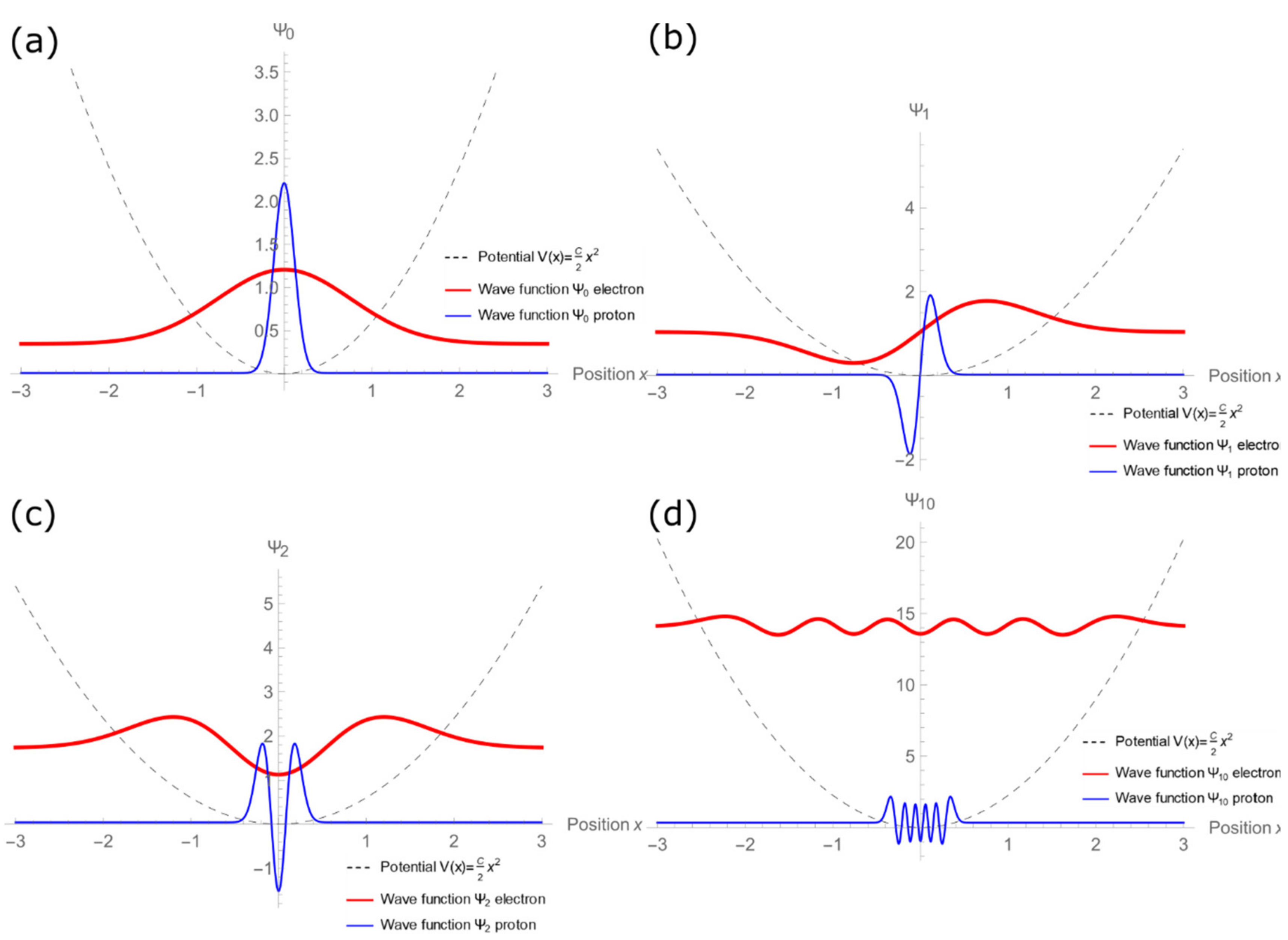
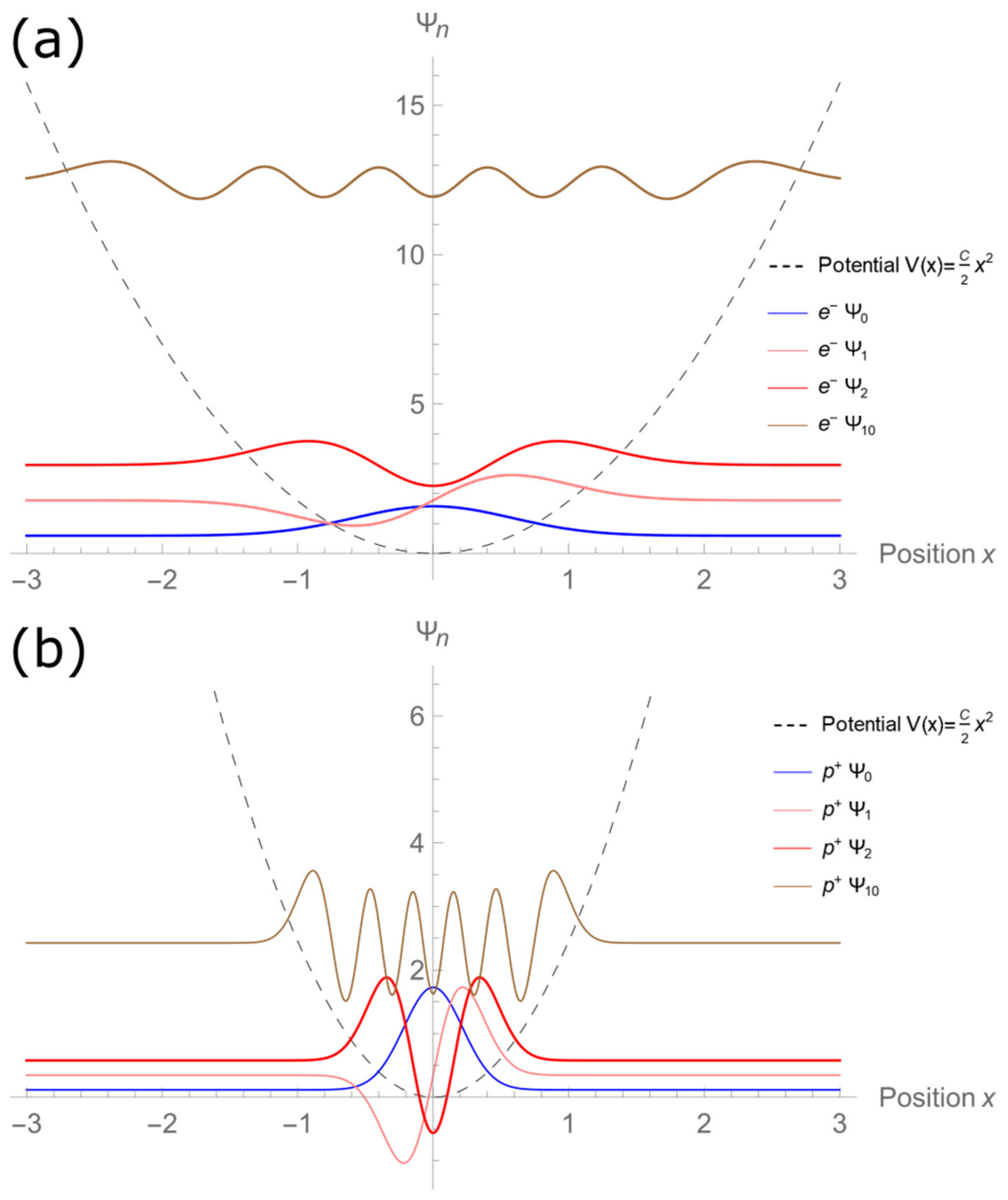
2.8. Normalization of the Eigenfunctions and Graph for Levels 0, 1, 2, and 10

In the previous eigenfunctions, the constant A 0 appears for the even solutions, and A 1 appears for the odd solutions. In this section, we will determine those constants by normalization. Normalization is defined as Ψ * x , t Ψ x , t   d x = 1 .
For time-independent potentials, we can express the wave function as Ψ x , t = ψ x e i ω t .
Its probability density is as follows: Ψ * x , t Ψ x , t = ψ 2 x ( e i ω t e + i ω t ) = ψ 2 x .
Consequently, the normalization for our wave functions will be ψ 2 x   d x = 1 .
In this case, we are dealing with time-independent Schrödinger wave functions. However, this methodology is equally valid for the normalization of time-dependent Schrödinger wave functions. The interested reader can consult the proof in Appendix D, which is based on the discussions presented in [27].
For n = 0 :
(a)
Square the function ψ 0 x : A 0 e α x 2 2 A 0 e α x 2 2 = A 0 2 e α x 2     ψ 0 2 x = A 0 2 e α x 2 ,
(b)
Integrate ψ 0 2 x from to : A 0 2 e α x 2 d x ,
This integral cannot be solved by analytical methods in variable x. However, in Appendix A, we present a detailed procedure of its analytical solution in polar coordinates. We give the result below:
A 0 2 e α x 2 d x = A 0 2 π α 1 2 ,
(c)
Determine the constant A 0 by equating the result of the previous integral to 1:
A 0 2 π α 1 2 = 1 A 0 2 = 1 π α 1 2 = α 1 2 π 1 2 A 0 = π α 1 4 ,
(d)
Write the wave function by inserting A 0 constant value into ψ 0 x :
ψ 0 x = A 0 e α x 2 2 w h e r e A 0 = α π 1 4 ψ 0 x = α π 1 4 e α x 2 2 .
For n = 1 :
(a)
Square the function ψ 1 x : ψ 1 x = A 1 α   x e α x 2 2     ψ 1 2 x = A 1 2 α   x 2 e α x 2 ,
(b)
Integrate ψ 1 2 x from to : A 1 2 α   x 2 e α x 2 d x     A 1 2 α x 2 e α x 2 d x ,
To solve this integral, it is necessary to use the function’s Γ definition. We describe in detail this procedure in Appendix B. We present the result below:
A 1 2 α x 2 e α x 2 d x = A 1 2 π 2 α ,
(c)
Determine the constant A 1 by equating the result of the previous integral to 1:
A 1 2 π 2 α = 1 A 1 2 = 2 α π A 1 = 2   α π 1 4 ,
(d)
Write the wave function by inserting A 1 constant value into ψ 1 x :
ψ 1 x = A 1 α   x e α x 2 2 ψ 1 x = 2 α π 1 4 α   x e α x 2 2 ; ψ 1 x = α π 1 4 2 α   x   e α x 2 2 .
For n = 2 :
(a)
Square the function ψ 2 x :
ψ 2 x = A 0 1 2 α   x 2 e α x 2 2 ; ψ 2 2 x = A 0 2 1 2 α   x 2 2 e α x 2 ,
(b)
Integrate ψ 2 2 x from to :
A 0 2 1 2 α   x 2 2 e α x 2 d x = 2 π α 1 2 A 0 2 ;
The function Γ is also involved in the solution of the latter integral. At this point, the student knows that one can rely on the mathematical formula book that is cited Appendix B [28] or on some mathematical software such as Wolfram Mathematica [29] to solve this kind of integral,
(c)
Determine the constant A 0 by equating the result of the previous integral to 1:
2 π α 1 2 A 0 2 = 1 A 0 2 = 1 2 α π 1 2 A 0 = 1 2 α π 1 4 ,
(d)
Write the wave function by inserting A 0 constant value into ψ 2 x :
ψ 2 x = A 0 1 2 α   x 2 e α x 2 2 ψ 2 x = 1 2 α π 1 4 1 2 α   x 2 e α x 2 2 ; ψ 2 x = α π 1 4 1 2 2 α   x 2 e α x 2 2 .
Before proceeding to the graphing of wave functions ψ 0 x , ψ 1 x , and ψ 2 x , let us discuss a particularity of normalized ψ 2 x wave function. In much of the available literature, the reader may find that ψ 2 x is written as follows:
ψ 2 x = α π 1 4 1 2 2 α x 2 1 e α x 2 2 .
The only difference between the two representations is the sign of the Hermite polynomial of order 2, 1 2 α x 2 = 2 α x 2 1 .
This is not an error that could have propagated through our procedure until our wave function ψ 2 x . Actually, the negative sign is related to the fact that in an “unaware” way, we select a 0 to be equal to one. We must not confuse the normalization constant A 0 with the coefficient a 0 of the Hermite polynomials.
In this regard, the physicists’ community has adopted a convention where the constants a 0 or a 1 are selected in such a way that allows the highest order power, in each Hermite polynomial, to appear positive.
For the case of our wave function ψ 2 x , it is only necessary to make a 0 = 1 . Following this convention and using the recursion relation of Equation (14) and the H u solutions of Equation (15), we present below the first 11 Hermite polynomials usable in the QHO.
H 0 u = 1 , H 1 u = u , H 2 u = 2 u 2 1 , H 3 u = 2 u 3 3 u , H 4 u = 4 u 4 12 u 2 + 3 , H 5 u = 4 u 5 20 u 3 + 15 u , H 6 u = 8 u 6 60 u 4 + 90 u 2 15 , H 7 u = 8 u 7 84 u 5 + 210 u 3 105 u , H 8 u = 8 u 8 112 u 6 + 420 u 4 420 u 2 + 105 , H 9 u = 16 u 9 288 u 7 + 1512 u 5 2520 u 3 + 945 u , H 10 u = 32 u 10 720 u 8 + 5040 u 6 12,600 u 4 + 9450 u 2 945 .
Therefore, our wave function for level n = 2 is as follows:
ψ 2 x = α π 1 4 1 2 2 α x 2 1 e α x 2 2 .
Furthermore, with the polynomials we have presented, it is relatively easy to obtain other wave functions. Let us do it for n = 10.
For n = 10 :
(a)
Write the general solution: ψ n u = A e u 2 2 H n u ,
(b)
In the last equation, insert H 10 u polynomial to get ψ 10 u :
ψ 10 u = A 0 32 u 10 720 u 8 + 5040 u 6 12,600 u 4 + 9450 u 2 945 e u 2 2 ,
(c)
Make the appropriate change of variable from u back to x :
u = α   x ; ψ 10 x = A 0 ( 32 α   x 10 720 α   x 8 + 5040 α   x 6 12,600 α   x 4 + 9450 α   x 2 945 ) e α x 2 2 ; ψ 10 x = A 0 32 α 5 x 10 720 α 4 x 8 + 5040 α 3 x 6 12,600 α 2 x 4 + 9450 α x 2 945 e α x 2 2 ,
(d)
Square the function ψ 10 x :
ψ 10 2 x = A 0 2 e α x 2 32 α 5 x 10 720 α 4 x 8 + 5040 α 3 x 6 12,600 α 2 x 4 + 9450 α x 2 945 2 ,
(e)
Integrate ψ 10 2 x from to :
ψ 10 2 x = 3,628,800 π α 1 2 A 0 2 ,
(f)
Determine the constant A 0 by equating the result of the previous integral to 1:
3,628,800 π α 1 2 A 0 2 = 1 A 0 = 1 720 7 α π 1 4 ,
(g)
Write the wave function by inserting A 0 constant value into ψ 10 x :
ψ 10 x = α π 1 4 1 720 7 32 α 5 x 10 720 α 4 x 8 + 5040 α 3 x 6 12,600 α 2 x 4 + 9450 α x 2 945 e α x 2 2 .
Figure 3a–d shows the wave functions graphs for n = 0, 1, 2, and 10. The energy eigenvalues are expressed as a function of the force constant C and the particle mass m. We have taken advantage of this to show the electron and proton wave functions simultaneously under the same potential V(x). Meanwhile, Figure 4 simultaneously presents the wave functions of levels n = 0, 1, 2, and 10 for electron (a) and proton (b) waves. In both, it is possible to identify the wave functions are evenly spaced.
The plots in Figure 3 and Figure 4 were made using Wolfram Mathematica software [28]. In Appendix C, we discuss the necessary considerations to make the graphs. We also present the short Mathematica code to reproduce our plots. The reader is free to use it to verify the present results. In case the reader does not have access to the Wolfram Mathematica software, we also provide web links to interactive plots.

3. Conclusions

We presented an eight-step procedure to solve the quantum harmonic oscillator analytically. The mathematical tools we used to this end are available in all Science, Technology, Engineering and Mathematics disciplines. Therefore, this solution is accessible not only for physics students but also for undergraduate engineering and chemistry students. We provided interactive web-based graphs for the reader to observe the shape of the wave functions for an electron and a proton when subject to the same potential V(x). Each of the eight steps in our solution procedure is self-contained; this allows the reader to consult any step of interest without the need to review the entire article.

Author Contributions

Conceptualization, A.R.-G.; methodology, A.R.-G.; software, A.R.-G.; validation, A.R.-G. and A.L.P.-M.; formal analysis, A.R.-G.; investigation, A.R.-G.; resources, A.R.-G.; data curation, A.R.-G. and A.L.P.-M.; writing—original draft preparation, A.R.-G. and A.L.P.-M.; writing—review and editing, A.R.-G. and A.L.P.-M.; visualization, A.R.-G. and A.L.P.-M.; supervision, A.R.-G.; project administration, A.R.-G.; funding acquisition, A.R.-G. All authors have read and agreed to the published version of the manuscript.

Funding

This research was funded by Investigación Científica Básica SEP—CONACYT 2016, grant number 283492 and PAPIIT-UNAM, grant number IN109020.

Acknowledgments

The authors acknowledge and appreciate the invaluable labor and courage of all those who, during the tragic COVID-19 pandemic, expose their lives to danger to keep doing essential activities for the good of all society. The first author acknowledges the funding received through the following projects: (a) Investigación Científica Básica SEP—CONACYT 2016, project number 283492; and (b) PAPIIT-UNAM, project number IN109020. Both authors declare their faith and gratitude to almighty God.

Conflicts of Interest

The authors declare no conflict of interest.

Appendix A. Analytic Solution of the Integral A 0 2 e α x 2 d x

Define the integral to be equal to I : I = A 0 2 e α x 2 d x .
Consequently, squaring I is equivalent to multiplying the integral by itself. Since it does not matter if we express the integrals in terms of the x or y variables, we will calculate I 2 using one integral in terms of x and the other in terms of y.
I 2 = A 0 4 e α y 2 e α x 2 d x d y , I 2 = A 0 4 e α x 2 α y 2 d x d y , I 2 = A 0 4 e α x 2 + y 2 d x d y .
The latter is an integral in the x-y plane going from to . However, if we express that same integral in polar coordinates, the x-y plane becomes the r- θ plane, and it goes from 0 to 2π in θ and from 0 to in r. Transformations from rectangular to polar coordinates are
x = r cos θ , y = r sin θ , r = x 2 + y 2 .
We identify immediately that it is possible to express the integrant e α x 2 + y 2 as e α r 2 .
Whenever we make a coordinate transformation, it is necessary to calculate the scale factor. This factor is the determinant of the Jacobian matrix J . Matrix J is
J = f 1 x 1 f 1 x 2 f 2 x 1 f 2 x 2 .
Since our coordinate transformation is x = r cos θ and y = r sin θ , then our Jacobian is
J = x ,   y r ,   θ = x r x θ y r y θ = r cos θ r r cos θ θ r sin θ r r sin θ θ = cos θ r sin θ sin θ r cos θ = r cos 2 + r sin 2 θ .
Because cos 2 + sin 2 θ = 1 , the scale factor for this coordinate transformation is precisely r.
Now, we can write I 2 as follows:
I 2 = A 0 4 0 0 2 π e α r 2 r d θ d r .
The integrand of the integral respect to θ is a constant. Therefore, we only have to integrate d θ from 0 to 2 π , I 2 = A 0 4 2 π 0 e α r 2 r   d r .
To integrate with respect to r, we should make a change of variable u = α r 2 ; d u = 2 α r   d r . With that change of variable, the limits of integration also change. The new lower limit remains 0; however, the upper limit becomes −∞. Therefore, we have
I 2 = A 0 4 2 π 1 2 α 0 e u   d u = A 0 4 2 π 2 α e u 0 = A 0 4 π α 0 1 = A 0 4 π α .
Recalling that our original integral is I and not I 2 , we must obtain the square root from the last result, I = A 0 4 π α 1 2 =   A 0 2 π α 1 2 .

Appendix B. Analytic Solution of the Integral A 1 2 α x 2 e α x 2 d x

For this integral, we should identify that the integrand function ( x 2 e α x 2 ) is an even function.
We have an even function if f(−x) = f(x). Even functions are symmetrical about the ordinate axis, and its integral from −∞ to ∞ is equivalent to twice its integral from 0 to ∞. As a result, we can write the following:
A 1 2 α   x 2 e α x 2 d x   = 2 A 1 2 α 0 x 2 e α x 2 d x .
To carry out the above integration, it should be remembered that gamma function is an extension of factorial function to the complex numbers and is defined as Γ z =   0 x z 1 e x d x .
The integral that we are trying to solve does not have the same form as the gamma function definition. Nevertheless, it has a very similar structure; thus, it is possible to express its solution using a particular gamma function arrangement. In [28], the reader will find countless useful formulas for solving these types of integrals. For the problem we are dealing with here, we have the following:
0 x m e a x 2 d x =   Γ m + 1 2 2 a m + 1 2 .
This latter formula has the exact form of the integral that we seek to solve with m = 2 and a = α . Thus,
2 A 1 2 α 0 x 2 e α x 2 d x = Γ 2 + 1 2 2 α 2 + 1 2 = Γ 3 2 2 α 3 2 . Since   Γ 3 2 = π 2 ,   we   have   2 A 1 2 α 0 x 2 e α x 2 d x = π 2 2 α 3 2 2 A 1 2 α = π 4 α 3 2 2 A 1 2 α = A 1 2 π 2 α .

Appendix C. Some Considerations and Wolfram Mathematica Code for the QHO Wavefunction Graphs

ψ n are functions whose variable is position x . The mathematical expressions for the wave functions we obtained in Section 2.8 include the parameter α. This is not a problem if we keep in mind what the value of α is α = 2 π m ν = m C m 1 2 = m C .
We can see that α will become a constant once we have specified one value for particle’s mass m and other for the potential force constant C . If we set = 1 for simplicity, then α = mC .
On the other hand, it should be noted that functions ψ n we obtained do not include the energy eigenvalue. Said value has to be added to the wave function as follows: E n + ψ n . In turn, E n is a constant, and, of course, it does not depend on the x position.
Like α , the energy eigenvalues E n also depend on the particle’s mass m and potential force constant C . To determine E n as a function of m and C , we will use the relation β α = 2 n + 1 , where α = 2 m π ν and β = 2 m E 2 .
We make = 1 for simplicity’s sake, then β = 2 m E , and α = m C . Consequently, β α = 2 m E m C . We set this last result equal to 2 n + 1 and resolve for E n .
2 m E m C = 2 n + 1     E n = 2 n + 1   m C 2 m .
If we do not get rid of by equating it to 1, we can identify that energy eigenvalues turn out to be E n = 2 n + 1   m C   2 m .
From the expressions of E n , we can identify that energy levels are evenly spaced, and when = 1 , they take the following values:
E 0 = m c 2 m ;   E 1 = 3 2 m c m ;   E 2 = 5 2 m c m ;   E 10 = 21 2 m c m .
In the graphs presented in Figure 3 and Figure 4, we have made that = 1 , C = 1.2 , and m = 2.5 .
Next, we present the code we used to make the graphs of Figure 3 and Figure 4. To use it, the reader just needs to copy and paste it into a Wolfram’s Mathematica notebook and then press the buttons `Shift’ and `Enter’ to execute it. The code generates a “manipulable” graph where it is possible to identify how ψ n evolves depending on the C and m values provided by the user. If the reader does not have access to Wolfram’s Mathematica software [29], the following links lead to interactive web-based graphs with the same traits.
For n = 0
Manipulate[
 Plot[{C/2*x^2,
   Sqrt[m*C]/(
    2*m) + ((m*Sqrt[C/m])^(1/4)  E^(-(1/2) (x^2 m*Sqrt[C/m])))/\[Pi]^(
    1/4), Sqrt[1836*m*C]/(
    1836*2*m) + ((1836*m*Sqrt[C/(1836*m)])^(1/4)
       E^(-(1/2) (x^2 1836*m*Sqrt[C/(1836*m)])))/\[Pi]^(1/4)}, {x, -3,
    3}, PlotStyle -> {{Dashed, Black, Thickness[0.001]}, {Red,
     Thickness[0.007]}, {Blue, Thickness[0.0035]}}, Axes -> True,
  AxesLabel -> {Position x, Subscript[\[CapitalPsi], 0]},
  PlotLegends -> {"Potential V(x)=\!\(\*FractionBox[\(C\), \(2\)]\)\!\
\(\*SuperscriptBox[\(x\), \(2\)]\)",
    "Wave function \!\(\*SubscriptBox[\(\[CapitalPsi]\), \(0\)]\) \
electron",
    "Wave function \!\(\*SubscriptBox[\(\[CapitalPsi]\), \(0\)]\) \
proton"}], {C, 1, 5}, {m, 0.05, 3}]
For n = 1
Manipulate[
 Plot[{C/2*x^2, (3*Sqrt[m*C])/(
    2*m) + ((m*Sqrt[C/m])^(1/4)  *Sqrt[2 m*Sqrt[C/m]]*x*
     E^(-(1/2) (x^2 m*Sqrt[C/m])))/\[Pi]^(1/4), (3*Sqrt[1836*m*C])/(
    1836*2*m) + ((1836*m*Sqrt[C/(1836*m)])^(1/4)  *Sqrt[
     1836*2 m*Sqrt[C/(1836*m)]]*x*
     E^(-(1/2) (x^2 1836*m*Sqrt[C/(1836*m)])))/\[Pi]^(1/4)}, {x, -3,
   3}, PlotStyle -> {{Dashed, Black, Thickness[0.001]}, {Red,
     Thickness[0.007]}, {Blue, Thickness[0.0035]}}, Axes -> True,
  AxesLabel -> {Position x, Subscript[\[CapitalPsi], 1]},
  PlotLegends -> {"Potential V(x)=\!\(\*FractionBox[\(C\), \(2\)]\)\!\
\(\*SuperscriptBox[\(x\), \(2\)]\)",
    "Wave function \!\(\*SubscriptBox[\(\[CapitalPsi]\), \(1\)]\) \
electron",
    "Wave function \!\(\*SubscriptBox[\(\[CapitalPsi]\), \(1\)]\) \
proton"}], {C, 1, 5}, {m, 0.05, 3}]
For n = 2
Manipulate[
 Plot[{C/2*x^2, (5*Sqrt[m*C])/(
    2*m) + ((m*Sqrt[C/m])^(
     1/4) (2 m*Sqrt[C/m] x^2 - 1) E^(-(1/2) (x^2 m*Sqrt[C/m])))/(
    Sqrt[2] \[Pi]^(1/4)), (5*Sqrt[1836*m*C])/(
    1836*2*m) + ((1836*m*Sqrt[C/(1836*m)])^(
     1/4) (1836*2 m*Sqrt[C/(1836*m)] x^2 - 1) E^(-(1/
       2) (x^2 1836*m*Sqrt[C/(1836*m)])))/(
    Sqrt[2] \[Pi]^(1/4))}, {x, -3, 3},
  PlotStyle -> {{Dashed, Black, Thickness[0.001]}, {Red,
     Thickness[0.007]}, {Blue, Thickness[0.0035]}}, Axes -> True,
  AxesLabel -> {Position x, Subscript[\[CapitalPsi], 2]},
  PlotLegends -> {"Potential V(x)=\!\(\*FractionBox[\(C\), \(2\)]\)\!\
\(\*SuperscriptBox[\(x\), \(2\)]\)",
    "Wave function \!\(\*SubscriptBox[\(\[CapitalPsi]\), \(2\)]\) \
electron",
    "Wave function \!\(\*SubscriptBox[\(\[CapitalPsi]\), \(2\)]\) \
proton"}], {C, 1, 5}, {m, 0.05, 3}]
For n = 10
Manipulate[
 Plot[{C/2*x^2, (21*Sqrt[m*C])/(
    2*m) + ((m*Sqrt[C/m])^(1/4)/(
      720 Sqrt[7] \[Pi]^(1/4)))*(32*(Sqrt[m*Sqrt[C/m]]*x)^10 -
       720*(Sqrt[m*Sqrt[C/m]]*x)^8 + 5040*(Sqrt[m*Sqrt[C/m]]*x)^6 -
       12600*(Sqrt[m*Sqrt[C/m]]*x)^4 + 9450*(Sqrt[m*Sqrt[C/m]]*x)^2 -
       945)* E^(-((x^2 m*Sqrt[C/m])/2)), (21*Sqrt[1836*m*C])/(
    1836*2*m) + ((1836*m*Sqrt[C/(1836*m)])^(1/4)/(
      720 Sqrt[7] \[Pi]^(
       1/4)))*(32*(Sqrt[1836*m*Sqrt[C/(1836*m)]]*x)^10 -
       720*(Sqrt[1836*m*Sqrt[C/(1836*m)]]*x)^8 +
       5040*(Sqrt[1836*m*Sqrt[C/(1836*m)]]*x)^6 -
       12600*(Sqrt[1836*m*Sqrt[C/(1836*m)]]*x)^4 +
       9450*(Sqrt[1836*m*Sqrt[C/(1836*m)]]*x)^2 - 945)*
     E^(-((x^2 1836*m*Sqrt[C/(1836*m)])/2))}, {x, -3, 3},
  PlotStyle -> {{Dashed, Black, Thickness[0.001]}, {Red,
     Thickness[0.007]}, {Blue, Thickness[0.0035]}}, Axes -> True,
  AxesLabel -> {Position x, Subscript[\[CapitalPsi], 10]},
  PlotLegends -> {"Potential V(x)=\!\(\*FractionBox[\(C\), \(2\)]\)\!\
\(\*SuperscriptBox[\(x\), \(2\)]\)",
    "Wave function \!\(\*SubscriptBox[\(\[CapitalPsi]\), \(10\)]\) \
electron",
    "Wave function \!\(\*SubscriptBox[\(\[CapitalPsi]\), \(10\)]\) \
proton"}], {C, 1, 5}, {m, 0.05, 3}]
For n = 0 , 1 , 2 , 10 electron
Manipulate[
 Plot[{C/2*x^2,
   Sqrt[m*C]/(
    2*m) + ((m*Sqrt[C/m])^(1/4)  E^(-(1/2) (x^2 m*Sqrt[C/m])))/\[Pi]^(
    1/4), (3*Sqrt[m*C])/(
    2*m) + ((m*Sqrt[C/m])^(1/4)  *Sqrt[2 m*Sqrt[C/m]]*x*
     E^(-(1/2) (x^2 m*Sqrt[C/m])))/\[Pi]^(1/4), (5*Sqrt[m*C])/(
    2*m) + ((m*Sqrt[C/m])^(
     1/4) (2 m*Sqrt[C/m] x^2 - 1) E^(-(1/2) (x^2 m*Sqrt[C/m])))/(
    Sqrt[2] \[Pi]^(1/4)), (21*Sqrt[m*C])/(
    2*m) + ((m*Sqrt[C/m])^(1/4)/(
      720 Sqrt[7] \[Pi]^(1/4)))*(32*(Sqrt[m*Sqrt[C/m]]*x)^10 -
       720*(Sqrt[m*Sqrt[C/m]]*x)^8 + 5040*(Sqrt[m*Sqrt[C/m]]*x)^6 -
       12600*(Sqrt[m*Sqrt[C/m]]*x)^4 + 9450*(Sqrt[m*Sqrt[C/m]]*x)^2 -
       945)* E^(-((x^2 m*Sqrt[C/m])/2))}, {x, -3, 3},
  PlotStyle -> {{Dashed, Black, Thickness[0.001]}, {Blue,
     Thickness[0.003]}, {Pink, Thickness[0.003]}, {Red,
     Thickness[0.003]}, {Brown, Thickness[0.003]}}, Axes -> True,
  AxesLabel -> {Position x, Subscript[\[CapitalPsi], n]},
  PlotLegends -> {"Potential V(x)=\!\(\*FractionBox[\(C\), \(2\)]\)\!\
\(\*SuperscriptBox[\(x\), \(2\)]\)",
    "\!\(\*SuperscriptBox[\(e\), \(-\)]\) \!\(\*SubscriptBox[\(\
\[CapitalPsi]\), \(0\)]\)",
    "\!\(\*SuperscriptBox[\(e\), \(-\)]\) \!\(\*SubscriptBox[\(\
\[CapitalPsi]\), \(1\)]\)",
    "\!\(\*SuperscriptBox[\(e\), \(-\)]\) \!\(\*SubscriptBox[\(\
\[CapitalPsi]\), \(2\)]\)",
    "\!\(\*SuperscriptBox[\(e\), \(-\)]\) \!\(\*SubscriptBox[\(\
\[CapitalPsi]\), \(10\)]\)"}], {C, 1, 5}, {m, 0.05, 3}]
For n = 0 , 1 , 2 , 10 proton
Manipulate[
 Plot[{C/2*x^2,
   Sqrt[1836*m*C]/(
    1836*2*m) + ((1836*m*Sqrt[C/(1836*m)])^(1/4)
       E^(-(1/2) (x^2 1836*m*Sqrt[C/(1836*m)])))/\[Pi]^(1/4), (
    3*Sqrt[1836*m*C])/(
    1836*2*m) + ((1836*m*Sqrt[C/(1836*m)])^(1/4)  *Sqrt[
     1836*2 m*Sqrt[C/(1836*m)]]*x*
     E^(-(1/2) (x^2 1836*m*Sqrt[C/(1836*m)])))/\[Pi]^(1/4), (
    5*Sqrt[1836*m*C])/(
    1836*2*m) + ((1836*m*Sqrt[C/(1836*m)])^(
     1/4) (1836*2 m*Sqrt[C/(1836*m)] x^2 - 1) E^(-(1/
       2) (x^2 1836*m*Sqrt[C/(1836*m)])))/(Sqrt[2] \[Pi]^(1/4)), (
    21*Sqrt[1836*m*C])/(
    1836*2*m) + ((1836*m*Sqrt[C/(1836*m)])^(1/4)/(
      720 Sqrt[7] \[Pi]^(
       1/4)))*(32*(Sqrt[1836*m*Sqrt[C/(1836*m)]]*x)^10 -
       720*(Sqrt[1836*m*Sqrt[C/(1836*m)]]*x)^8 +
       5040*(Sqrt[1836*m*Sqrt[C/(1836*m)]]*x)^6 -
       12600*(Sqrt[1836*m*Sqrt[C/(1836*m)]]*x)^4 +
       9450*(Sqrt[1836*m*Sqrt[C/(1836*m)]]*x)^2 - 945)*
     E^(-((x^2 1836*m*Sqrt[C/(1836*m)])/2))}, {x, -3, 3},
  PlotStyle -> {{Dashed, Black, Thickness[0.001]}, {Blue,
     Thickness[0.002]}, {Pink, Thickness[0.002]}, {Red,
     Thickness[0.003]}, {Brown, Thickness[0.002]}}, Axes -> True,
  AxesLabel -> {Position x, Subscript[\[CapitalPsi], n]},
  PlotLegends -> {"Potential V(x)=\!\(\*FractionBox[\(C\), \(2\)]\)\!\
\(\*SuperscriptBox[\(x\), \(2\)]\)",
    "\!\(\*SuperscriptBox[\(p\), \(+\)]\) \!\(\*SubscriptBox[\(\
\[CapitalPsi]\), \(0\)]\)",
    "\!\(\*SuperscriptBox[\(p\), \(+\)]\) \!\(\*SubscriptBox[\(\
\[CapitalPsi]\), \(1\)]\)",
    "\!\(\*SuperscriptBox[\(p\), \(+\)]\) \!\(\*SubscriptBox[\(\
\[CapitalPsi]\), \(2\)]\)",
    "\!\(\*SuperscriptBox[\(p\), \(+\)]\) \!\(\*SubscriptBox[\(\
\[CapitalPsi]\), \(10\)]\)"}], {C, 1, 5}, {m, 0.05, 3}]

Appendix D. Normalization Proof for Time-Dependent Schrödinger Wave Functions

We will consider a one-dimensional wave function, i.e., a function of position x and time t .
We know that the absolute value of the square of the wave function is proportional to its probability density. For the case of a wave function like the one we are proposing, ψ x ,   t , the probability density gives us the probability of finding the particle at a given time t in the interval x 2 > x > x 1 .
We can write the above in the following way:
P x 1 , x 2 = A x 1 x 2 ψ x , t 2 d x .
For the previous expression, A is a constant that does not depend on the variable x .
Of course, we can determine constant A by saying that the probability of finding the particle somewhere in space is equal to 100%; i.e.,
1 = A + ψ x , t 2 d x .
It could happen that the integral of the previous equation does not converge. In this case, the constant A would have to be zero, and therefore the equality of Equation (A2) would not be satisfied.
However, seeing Equation (A1), we would know that if A = 0 , it would mean that the probability of finding the particle in any finite interval must also be zero.
As the above does not correspond to situations that have a physical meaning, we come to an important conclusion: if ψ   x ,   t is a wave function that we want to use for Schrödinger wave mechanics, then   ψ   x ,   t     2 must be an integrable function of x for all values of t .
From the above, we impose the condition that integral of Equation (A2) must converge.
Now that the square of ψ   x ,   t is “integrable”, we can define a new wave function, ψ n x ,   t , as follows:
ψ a x , t = A ψ x , t ,
where A can be obtained from Equation (A2).
The wave function ψ a x ,   t from Equation (A3) has the property that
+ ψ a x , t 2 d x = 1   ;   P x 1 , x 2 = x 1 x 2 ψ a x , t 2 d x .
That is, the probability density is equal to the absolute value of ψ a x ,   t squared.
If there is a function ψ a x ,   t that satisfies the first equation of expression Equation (A4), then we can call that ψ a x ,   t a normalizable wave function.
Now let us recall that we start this discussion by assuming that the wave function ψ   x ,   t is a function that satisfies the Schrödinger equation; i.e.,
  2 m 2 x 2 ψ x , t + V x ψ x , t = i t ψ x , t .
However, in Equation (A3), we define a new wave function ψ a x ,   t .
ψ a x ,   t also satisfies the Schrödinger equation as long as the constant A is not time-dependent.
Let us proceed to our analysis by stating the following:
If ψ   x ,   t satisfies Equation (A5) and also tends to zero as x tends to + or , then
d d t + d x ψ x , t   2 = 0 .
To prove the previous theorem, we differentiate the function that is inside the integral in the following way:
t ψ x , t 2 = t ψ * x , t   ψ x , t .
Applying the product rule, we have
t ψ x , t 2 = ψ * x , t ψ x , t t + ψ * x , t t   ψ x , t .
Observe that on the right side of Equation (A5), we find an expression that is the partial derivative with respect to time of the function ψ   x ,   t .
Meanwhile, in Equation (A7), we have the partial derivative with respect to time of the complex conjugate of ψ   x ,   t , i.e., ψ * x , t t .
If we take the complex conjugate from Equation (A5), we can obtain an expression for ψ * x , t t , and so
i t ψ * x , t = 2   2 m 2 x 2 ψ * x , t V x ψ * x , t .
Observe that in the previous expression, we leave the function V   x unchanged; this is because we assume that V   x is not a complex function but a real one. This makes total sense for any classical problem in Schrödinger wave mechanics since the potentials that a particle “faces” are real.
Now, from Equation (A5), we solve for t ψ x , t :
t ψ x , t = i   2 m 2 x 2 ψ x , t i V x   ψ x , t .
We also solve t ψ * x , t from Equation (A8):
t ψ * x , t = i 2 m 2 x 2 ψ * x , t + i V x ψ * x , t .
We evaluate Equations (A9) and (A10) in Equation (A7):
t ψ x , t 2 = ψ * x , t i   2 m 2 x 2 ψ x , t i V x   ψ x , t +   ψ x , t i 2 m 2 x 2 ψ * x , t + i V x ψ * x , t t ψ x , t 2 = i   2 m ψ * x , t 2 x 2 ψ x , t i ψ * x , t V x ψ x , t i   2 m ψ x , t 2 x 2 ψ * x , t + i ψ x , t V x ψ * x , t = i 2 m ψ * x , t 2 x 2 ψ x , t   ψ x , t 2 x 2 ψ * x , t ,
which we can also write as
t ψ x , t 2 = i 2 m x ψ * x , t ψ x , t x   ψ x , t ψ * x , t x .
Let us rewrite Equation (A2) again:
d d t + d x ψ x , t   2 = 0 .
As we had already mentioned, we can put the differential operator d d t inside the integral; therefore,
+   t d x ψ x , t 2 = 0 .
We can arrange the differential operator t to operate on ψ x , t 2 as follows:
+ d x   t ψ x , t 2 = 0 .
We evaluate the result of Equation (A11) in this last expression as follows:
+   i 2 m x ψ * x , t ψ x , t x   ψ x , t ψ * x , t x d x = 0 .
Taking the constants out of the integral, we have
i 2 m + x ψ * x , t ψ x , t x   ψ x , t ψ * x , t x   d x = 0 .
In the integrand, we have the derivative of some functions, which can be interpreted as the integral “canceling” the derivative; therefore, we can safely write
i 2 m ψ * x , t ψ x , t x   ψ x , t ψ * x , t x + .
Using this last result, we can write
d d t + d x ψ x , t   2 = i 2 m ψ * x , t ψ x , t x   ψ x , t ψ * x , t x + .
Although we do not evaluate the derivatives enclosed in square brackets, we know that the right-hand side of Equation (A12) will disappear because, from the beginning, we had assumed that ψ x , t becomes zero at x = ± .
Therefore, the theorem of Equation (A6) is consistent, and consequently, the A of Equation (A2) is a constant independent of time.
All of this tells us that the function ψ a x , t is also a genuine Schrödinger wave function or, in other words, a solution to the Schrödinger equation.
So, we can always form a normalized wave function from a given wave function, and if it is convenient, we can work with functions normalized to 1 [27].
All this discussion is valid for the three-dimensional case, and its proof is analogous to the one we present for the one-dimensional case.
It is worth making a final consideration regarding the following wave function:
ψ x , t = e i x p i t p 2 2 m .
This is a function whose square is not integrable (in the terms we have already discussed), and so, according to our discussion, it is not a normalizable wave function.
The above prompts us to conclude that a precisely defined momentum wave function that depends on the independent variable x through the exponential function e i x p does not correspond to a physical state of “realizable” motion of the particle.
Nevertheless, we are not prevented from considering a wave that, over a very large interval on the x axis, depends on x through the factor e i x p , provided that this wave function tends to zero as x tends to + or .
For this reason, we can solve our dilemma if we agree that when we talk about waves with precisely defined momentum, it does not mean that the wave is actually everywhere with a shape e i x p .
We are aware that the wave function must tend to zero at infinity, but we assume that the wave function is in this form over a very large interval of the x -axis that includes the region in which we are most interested. Therefore, the monochromatic waves in Equation (A13) must be understood as almost monochromatic waves. With this clarification, we can continue talking about waves that depend on the independent variables x and t through the factors e i x p just like it is done in most quantum mechanics texts.
We can consider normalized waves as limit cases of normalizable waves, and if we want, we can refer to functions belonging to this last wave function type as “improper wave functions”. The term “improper wave functions” is also useful for soothing mathematical rigorists who could be alarmed about how physicists talk about and use the term plane wave as if they were genuine Schrödinger wave functions [27].

References

  1. Lyshevski, S.E.; Andersen, J.D.; Boedo, S.; Fuller, L.; Raffaelle, R.; Savakis, A.; Skuse, G.R. Multidisciplinary Undergraduate Nano-Science, Engineering and Technology Course. In Proceedings of the 2006 Sixth IEEE Conference on Nanotechnology, Cincinnati, OH, USA, 17–20 July 2006. [Google Scholar]
  2. Chari, D.; Howard, R.; Bowe, B. Disciplinary Identity of Nanoscience and Nanotechnology Research-A Study of Postgraduate. Int. J. Digit. Soc. 2012, 3, 614–621. [Google Scholar] [CrossRef]
  3. Thornton, S.T.; Rex, A. Modern Physics for Scientists and Engineers; Cengage Learning ALL: Boston, MA, USA, 2013. [Google Scholar]
  4. Beiser, A. Concepts of Modern Physics; McGraw-Hill Higher Education: New York, NY, USA, 2003. [Google Scholar]
  5. Tipler, P.A.; Llewellyn, R.A. Modern Physics; W. H. Freeman and Company: New York, NY, USA, 2008. [Google Scholar]
  6. Serway, R.A.; Moses, C.J.; Moyer, C.A. Modern Physiscs; Thomson Learning: Belmont, CA, USA, 2005. [Google Scholar]
  7. Levine, I.N. Quantum Chemistry; Pearson Education, Inc.: Saddle River, NJ, USA, 2014. [Google Scholar]
  8. Taylor, P.L.; Heinonen, O. A Quantum Approach to Condensed Matter Physics; Cambridge University Press: New York, NY, USA, 2002. [Google Scholar]
  9. Brehm, J.J.; Mullin, W.J. Introduction to the Structure of Matter: A Course in Modern Physics; John Wiley & Sons, Inc.: Hoboken, NJ, USA, 1989. [Google Scholar]
  10. Shankar, R. Principles of Quantum Mechanics; Plenum Publishers/Kluwer Academic: New York, NY, USA, 1994. [Google Scholar]
  11. Liboff, R.L. Introductory Quantum Mechanics; Longman Higher Education: Boston, MA, USA, 1987. [Google Scholar]
  12. Cohen-Tannoudji, C.; Diu, B.; Laloe, F. Quantum Mechanics; Wiley-Interscience: New York, NY, USA, 1991. [Google Scholar]
  13. Dirac, P.A.M. The Principles of Quantum Mechanics; Oxford University Press: Oxford, UK, 1958. [Google Scholar]
  14. Kato, T.; Tanimura, Y. Two-dimensional Raman and infrared vibrational spectroscopy for a harmonic oscillator system nonlinearly coupled with a colored noise bath. J. Chem. Phys. 2004, 120, 260–271. [Google Scholar] [CrossRef] [PubMed] [Green Version]
  15. Boyer, T.H. Thermodynamics of the harmonic oscillator: Wien’s displacement law and the Planck spectrum. Am. J. Phys. 2003, 71, 866–870. [Google Scholar] [CrossRef] [Green Version]
  16. Marquardt, R.; Quack, M. Radiative excitation of the harmonic oscillator with applications to stereomutation in chiral molecules. Z. Phys. D Atoms. Mol. Clust. 1996, 36, 229–237. [Google Scholar] [CrossRef]
  17. Suárez, E.; Díaz, N.; Suárez, D. Entropy Calculations of Single Molecules by Combining the Rigid–Rotor and Harmonic-Oscillator Approximations with Conformational Entropy Estimations from Molecular Dynamics Simulations. J. Chem. Theory Comput. 2011, 7, 2638–2653. [Google Scholar] [CrossRef] [PubMed]
  18. Gasiorowicz, S. Quantum Physics; John Wiley & Sons, Ltd.: Essex, MA, USA, 2003. [Google Scholar]
  19. Eisberg, R.; Resnick, R. Quantum Physics of Atoms, Molecules, Solids, Nuclei and Particles; John Wiley & Sons, Ltd.: New York, NY, USA, 1985. [Google Scholar] [CrossRef]
  20. Ghatak, A.; Lokanathan, S. Quantum Mechanics: Theory and Applications; Springer: Dordrecht, The Netherlands, 2004. [Google Scholar] [CrossRef]
  21. Denny, M. Harmonic oscillator quantization: Kinetic theory approach. Eur. J. Phys. 2002, 23, 183–190. [Google Scholar] [CrossRef]
  22. Viana-Gomes, J.; Peres, N.M.R. Solution of the quantum harmonic oscillator plus a delta-function potential at the origin: The oddness of its even-parity solutions. Eur. J. Phys. 2011, 32, 1377–1384. [Google Scholar] [CrossRef] [Green Version]
  23. Pimentel, D.R.M.; de Castro, A.S. A Laplace transform approach to the quantum harmonic oscillator. Eur. J. Phys. 2013, 34, 199–204. [Google Scholar] [CrossRef] [Green Version]
  24. Nogueira, P.H.F.; de Castro, A.S. Revisiting the quantum harmonic oscillator via unilateral Fourier transforms. Eur. J. Phys. 2016, 37, 015402. [Google Scholar] [CrossRef] [Green Version]
  25. Borghi, R. Quantum harmonic oscillator: An elementary derivation of the energy spectrum. Eur. J. Phys. 2017, 38, 025404. [Google Scholar] [CrossRef]
  26. Pérez-Jordá, J.M. On the recursive solution of the quantum harmonic oscillator. Eur. J. Phys. 2018, 39, 015402. [Google Scholar] [CrossRef] [Green Version]
  27. Wichmann, E.H. Quantum Physics. In Berkeley Physics Course; Mcgraw-Hill College: New York, NY, USA, 1971; Volume 4. [Google Scholar]
  28. Spiegel, M.R.; Liu, J. Schaum’s Mathematical Handbook of Formulas and Tables; McGraw-Hill Education: New York, NY, USA, 2008. [Google Scholar]
  29. Mathematica; Version 12.1; Software For Technical Computation; Wolfram Research: Champaign, IL, USA, 2020.
Figure 1. (a) A “realistic” continuous potential is described by the solid gray line. At the minimum, the “realistic” potential can be very well approximated by a quadratic potential (dashed black line). (b) By setting the origin of the coordinate system at the minimum of the dashed quadratic potential, we redefine the zero-potential energy V 0 = 0.
Physics 02 00031 g001
Figure 2. In this figure, we observe a central forces problem. It can be modeled as a single particle problem of reduced mass µ. For simplicity, we will consider particle 1 to be anchored while particle 2 oscillates with amplitude x.
Physics 02 00031 g002
Figure 3. Electron and proton wave functions, when subjected to the same V(x) = (C/2)x2 potential, for (a) n = 0, (b) n = 1, (c) n = 2, and (d) n = 10. It is possible to identify that the electron wave has greater penetration in the classically excluded region than the proton wave.
Physics 02 00031 g003
Figure 4. Wave functions of levels n = 0, 1, 2, and 10 for (a) electron particle and (b) proton particle. In both cases, it is possible to identify that the wave functions of consecutive levels are evenly spaced.
Physics 02 00031 g004
Publisher’s Note: MDPI stays neutral with regard to jurisdictional claims in published maps and institutional affiliations.

