Initial Studies of Electron Beams as a Means of Modifying Collagen

Abstract

We present the initial design studies and specifications for an accelerator and conveyor system to irradiate collagen samples, modifying properties such as the putrescibility and mechanical behaviours in a paradigm shift from existing, widely used technology. We show the integrated design requirements for a magnetic rastering scheme to move the beam position in order to ensure a uniform dose distribution over the full surface of the hide and discuss its dependence on factors such as the size of the hide, the beam current and conveyor speed. We also present initial energy deposition studies using beam particle interaction simulation program G4beamline, in order to determine the numerical beam parameters and angle of incidence needed to ensure a uniform depth-dose distribution throughout the hide thickness.

1. Introduction

Particle accelerators are used for a wide range of applications, such as high energy physics experiments [1,2,3], which are very high profile, but account for less than 1% of all the particle accelerators in operation. The vast majority of accelerators are used for more subtle applications, but have an enormous impact on everyday life. These accelerators are primarily used for security, medical and industrial applications, such as cargo scanning, cancer therapy and manipulating the physical properties of polymers, such as creating thermosetting plastics. In a world with an increasing demand for green technology and sustainability, particle accelerators have great potential for developing disruptive technologies in this respect. This study focuses on the main industrial use of collagen modification, namely leather manufacture, but there are other applications that could utilise this technology.

The leather production process consists of multiple stages, many of which require non-benign chemicals and can have a long-term impact on the local environment if not properly treated and disposed [4,5,6]. Many countries in the developed world such as the USA and EU states [7,8] have stringent regulations to ensure that by-products from leather production are disposed of with minimal impact on the local environment. In developing countries, tanneries often have difficulty in meeting the requirements of the regulations.

Leather manufacture is a global, multi-billion dollar industry that involves numerous steps to transform a skin/hide into a piece of finished leather ready for conversion into a product. The number of steps and chemicals involved vary enormously depending on the end use of the leather, but there are normally common steps involved in all processes; one of which is tanning. The tanning process consists of using tanning agents to create branching between protein chains. This process is qualitatively similar to the cross-linking of polymers, which is readily achieved by mixing polymers with cross-linking agents and irradiating with electron beams.

The use of electron beams for collagen modification and in particular leather tanning has several potential advantages over existing technology. One of the more high-profile components used in leather manufacture is chromium with over 80% of the worlds leather containing it. One key advantage of electron beam (e-beam) tanning is that water consumption and the quantities of tannages used in the tanning process can be substantially reduced, with chromium uptake efficiencies reaching close to 100%; this process also allows for simpler recycling of unused tanning agents. It is also expected that tanning would be able to occur over a wider range of temperatures and pH, while also allowing for the use of novel tanning agents that would typically be too unstable in water or air to bind to the collagen.

The uniformity of the tanning reaction throughout the cross-section of a skin/hide is crucial for the end product to achieve tight specification parameters set by the original equipment manufacturers (OEMs), as well as meeting legislative restrictions. This requires optimisation of the dose distribution over the surface of the hide, as well as ensuring a uniform depth-dose distribution. At present, studies into this process are ongoing, and as such, the viability of this novel process is under investigation.

As discussed in Section 3, in order to optimise the depth-dose curve, the energy spectrum of the beam and/or the angle of incidence of the beam at the hide surface must be tailored. A simple but costly way to achieve this is to use multiple accelerators with different energies or angles of incidence. A sophisticated but more cost-effective approach would be to kick out some bunches from the linac at different energies or to deflect certain bunches by differing amounts with the use of fast kickers and septum magnets [9,10]. A simple, inexpensive but laborious and slower option is to irradiate the hide multiple times with different irradiation angles and/or energies. In the last option, the conveyor belt can be designed to tilt the hide to different angles. The conveyor belt would go back and forth with different angles. The irradiation time and thus conveyor belt would be adjusted according to the mix ratio.

This paper presents a theoretical study of the design of the beam rastering scheme, which is required to scan the electron beam over the surface of the hide to ensure a uniform dose distribution over the hide surface. This is presented in Section 2. Section 3 presents simulation results of dose deposition through the thickness of the hide and determines the required beam energy spectrum, as well as the required angle of incidence of the beam in order to ensure a uniform depth-dose curve. Hence, the overall studies in this paper ensure that the dose deposition throughout the volume of the hide is as uniform as possible.

2. Design Considerations

2.1. Irradiation System Layout

The layout of the irradiation system is as shown in Figure 1. The accelerator is located on the top, and the electron beam is directed downward. A raster dipole magnet is located after the exit of the accelerator to bend the beam. The field of the magnet is varied rapidly to scan the beam along the surface of the hide.

The accelerator cavity is kept in the vacuum, and the hide is in the air. A vacuum chamber is placed at the exit of the accelerator and between the pole gap of the magnet to shorten the distance beam travels in the air. The scanned beam travels inside the vacuum chamber and exits through a vacuum window (thin metal foil) at the other end. The beam then travels another 5–10 cm in the air before reaching the hide placed on the conveyor belt. The belt moves in a direction perpendicular to the scanning surface. As the required beam energy is relatively low, the magnetic field strengths required are also low, and hence, a soft magnetic material would be most appropriate for the core of the raster magnet, so the field error due to the hysteresis is insignificant.

2.2. Orientation of the Target with Respect to the Beam

As we discuss in this paper, the dose deposition curve of an electron beam can be altered by either changing the energy of the beam or by varying the angle of incidence of the electron beam on the target. The simulation studies shown in the next section indicate that, qualitatively, varying the energy and the angle of incidence has a similar effect on the dose deposition.

We made no assumptions on the preferred means of varying the dose deposition through the hide; instead, we simply present different possibilities that allow different options to be considered in later studies. This section considers the possibilities for varying the angle of incidence of the electron beam, taking into account the challenges faced.

A whole hide from a fully grown bull is approximately $2\times 2.5$ m${}^2$ in size, and if the intention is to irradiate the entire hide in one piece, then the electron beam must be scanned over the entire width. When a charged particle travels through a uniform magnetic field orientated perpendicular to the direction of motion, as with a dipole magnet, the particle adopts a circular path, with radius of curvature $\rho$. 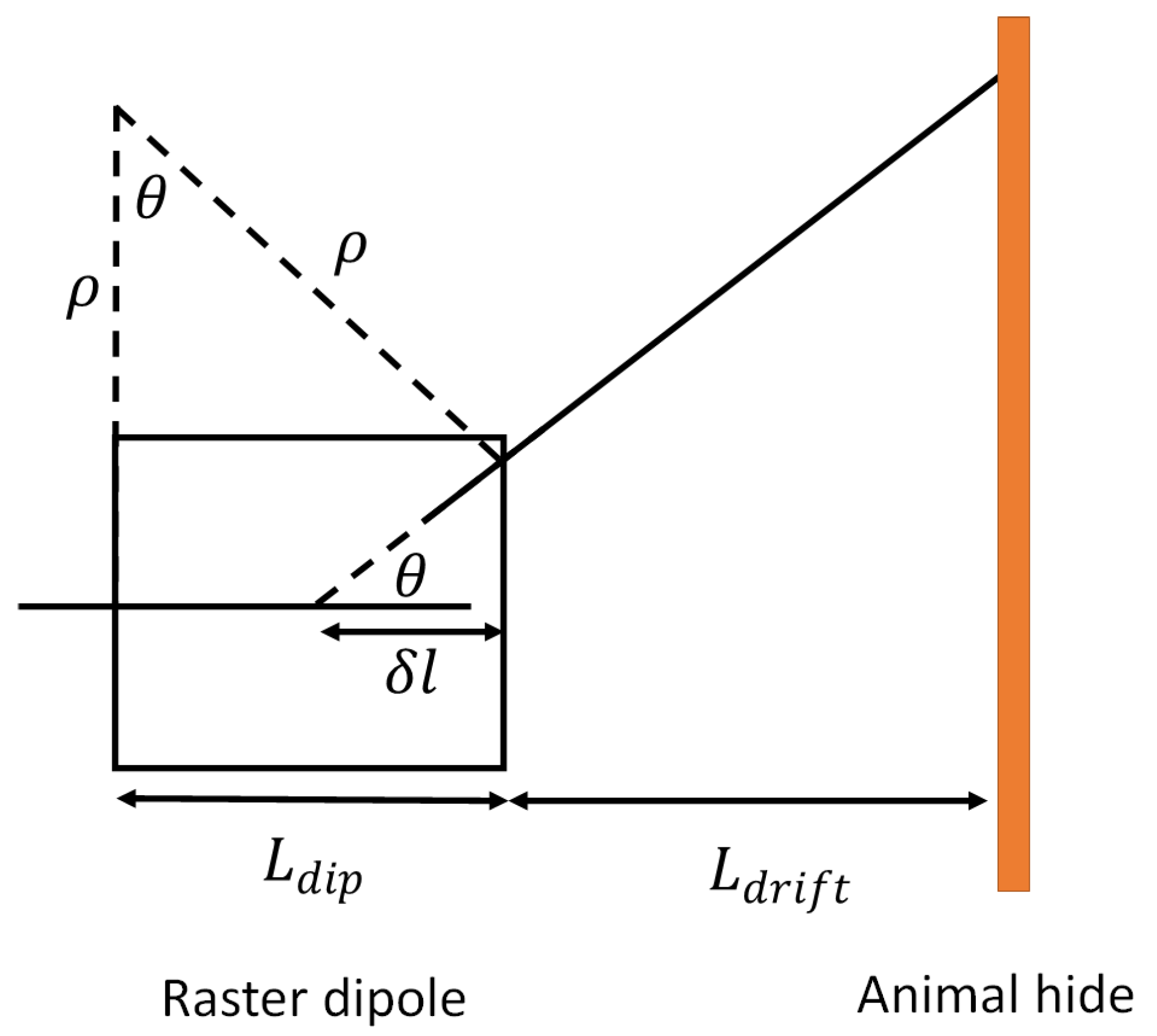Figure 2 shows a schematic diagram of the geometry of the beam trajectory through the raster scanning magnet to the hide. We define $\theta$ as the bending angle, $l_{\mathrm{dip}}$ as the dipole length and $L_{\mathrm{drift}}$ as the distance between the scanning magnet and the centre of the hide.

Figure 2 considers the position, z, to be the apparent point of rotation of the beam. That is to say that we know that before and after the dipole magnet, the electron beam trajectory is a straight line, so rather than considering the true curved path of the trajectory through the dipole magnet, we can consider that at some location, the beam is rotated by an angle $\theta$. We know that the radius of curvature is given as:

$$\rho =\frac{l_{\mathrm{dip}}}{sin\theta }.$$

(1)

We also know that the offset of the electron beam at the exit of the raster magnet (where we take $x>0$ to be to the right of the beam at the entrance of the raster magnet) is given as:

$$x_{\mathrm{off}}=\rho \left(1-cos\theta \right)=l_{\mathrm{dip}}\frac{1-cos\theta }{sin\theta }.$$

(2)

In terms of $\theta$, the gradient of the line after the raster magnet is given as $\frac{dy}{dx}=tan\theta$, and from this, we obtain:

$$\delta l=\frac{x_{\mathrm{off}}}{tan\theta }=l_{\mathrm{dip}}\frac{cos\theta \left(1-cos\theta \right)}{{sin}^2\theta }=l_{\mathrm{dip}}\frac{cos\theta }{1+cos\theta }.$$

(3)

From this, if we define the position of the beam at the start of the raster magnet as $\left(x,y\right)=\left(0,0\right)$, then the point of rotation is given as $\left(x,y\right)=\left(\frac{l_{\mathrm{dip}}}{1+cos\theta },0\right)$. The point of rotation is not at a fixed position, but rather, it varies with the angle, with the position changing more as $\theta$ increases.

In order to ensure that we achieve uniform tanning across the hide, we need to ensure that the angle of incidence between the beam and the normal to the surface of the hide is constant across the full scanning range of the beam. It should also be noted that when designing the magnetic rastering scheme, we shall also require that the beam scans over the surface of the hide at a constant rate as well.

We define the angle of incidence of the beam, $\varphi$, to be the angle between the beam trajectory and the normal to the surface of the hide. For two lines with gradients $m_1=tan\theta$ and $m_2=\frac{dy}{dx}$, where the angle of intersection between the lines is $\left(\frac{\pi }{2}-\varphi \right)$, then we have:

$$m_1{m}_2+1=\sqrt{m_1^2+1}\sqrt{m_2^2+1}cos\left(\frac{\pi }{2}-\varphi \right),$$

(4)

from which we obtain the gradient of the hide as a function of $\theta$ and $\varphi$ as:

$$\frac{dy}{dx}=-\frac{1}{tan\left(\theta \pm \varphi \right)}.$$

(5)

The choice of sign in Equation (5) is based on which direction we define angles to be positive. For this paper, we chose the positive sign convention, but this is a completely free choice. We also know the equation of the line defining the trajectory of the beam between the raster magnet and the hide must be:

$$y=xtan\theta -\frac{l_{\mathrm{dip}}sin\theta }{cos\theta \left(1+cos\theta \right)}.$$

(6)

Let us now assume that points $\left(x,y\right)$ and $\left(x+\delta x,y+\delta y\right)$ are points on the surface of the hide that are sufficiently close together such that we can assume a straight line between them, then from Equations (5) and (6), we have:

$$\begin{array}{c}\delta y=-{\displaystyle \frac{\delta x}{tan\left(\theta +\varphi \right)}}\hfill \\ =\left(x+\delta x\right)tan\left(\theta +\delta \theta \right)-{\displaystyle \frac{l_{\mathrm{dip}}sin\left(\theta +\delta \theta \right)}{cos\left(\theta +\delta \theta \right)\left(1+cos\left(\theta +\delta \theta \right)\right)}}-xtan\theta +{\displaystyle \frac{l_{\mathrm{dip}}sin\theta }{cos\theta \left(1+cos\theta \right)}}.\hfill \end{array}$$

(7)

From Equations (5) and (7), it can be shown that:

$$\begin{array}{c}{\displaystyle \frac{dx}{d\theta }}=-\left(x-{\displaystyle \frac{l_{\mathrm{dip}}\left(1+cos\theta -{cos}^2\theta \right)}{1+cos\theta }}\right)\left(tan\theta +tan\varphi \right),\hfill \\ \\ {\displaystyle \frac{dy}{d\theta }}=\left(y-{\displaystyle \frac{l_{\mathrm{dip}}\left(1-cos\theta \right)}{sin\theta \left(1+cos\theta \right)}}\right)\left(cot\theta -tan\varphi \right).\hfill \end{array}$$

(8)

The differential equations given in Equation (8) need to be solved numerically; however, we can make some approximations to allow us to gain some insight into the approximate form of the solution. If we assume that $L_{\mathrm{drift}}\gg l_{\mathrm{dip}}$, then we can neglect the variation in the point of rotation as the deflection angle of the raster magnet is varied. In this assumption, we obtain the simplified differential equations:

$$\begin{array}{c}{\displaystyle \frac{dx}{d\theta }}=-x\left(tan\theta +tan\varphi \right),\hfill \\ \\ {\displaystyle \frac{dy}{d\theta }}=y\left(cot\theta -tan\varphi \right).\hfill \end{array}$$

(9)

which can easily be solved and provide the general solution:

$$\begin{array}{c}x=L_{\mathrm{drift}}{e}^{-\theta tan\varphi }cos\theta ,\hfill \\ y=L_{\mathrm{drift}}{e}^{-\theta tan\varphi }sin\theta .\hfill \end{array}$$

(10)

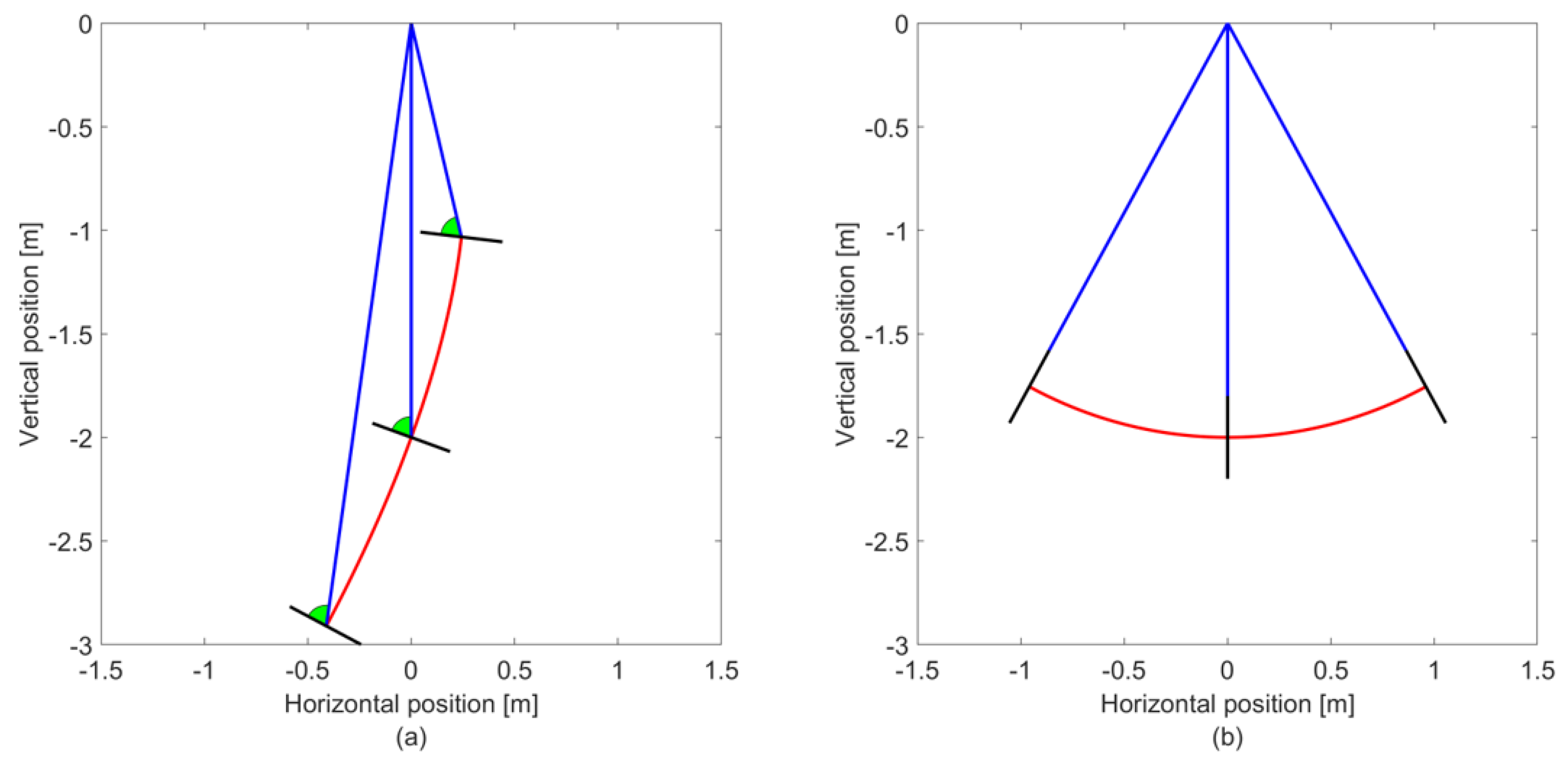
This solution describes the general equation for an exponential spiral, which is a set of curves, including the Golden Spiral, which have the property that for a line passing through the origin and intersecting the spiral, the angle of intersection is a constant. We see that when we apply simplifications to Equation (8), it produces the correct result as expected. Figure 3 shows a diagram of the hide orientation for an angle of incidence of ${70}^{\circ }$ (a) and $0^{\circ }$ (b), based on Equation (10) and assuming that the point of rotation is independent of the deflection angle, which is a reasonable assumption in this case. In both figures, we can see that the angle of incidence remains constant regardless of the deflection angle of the beam. The blue lines represent the direction of the electron beam, the black lines the normal to the hide surface and the red line the hide, and the green areas demonstrate that the angle of incidence remains constant for non-zero angles of incidence.

When $\varphi \ne 0$, the angular range of the beam will not be symmetric. We would either have to shift the midpoint of the hide transversely or apply a DC offset current to the scanning magnet to shift the range of the angles. In practice, the latter option is likely to be the preferred solution.

So far, we considered the case where the hide is curved in the deflecting plane of the beam in order to ensure that the angle of incidence remains constant. We could also imagine inclining the plane of the hide as it passes through the electron beam; however, we would still need to ensure that the angle of incidence in the deflecting plane is zero to ensure we have the angle of incidence we expect; thus, we would need to solve Equation (8) for $\varphi =0$.

2.3. Design of the Rastering Scheme

The rastering scheme needs to be able to ensure that the beam is swept over the surface of the hide in a uniform manner. For this, there are several key considerations we need to take into account. Firstly, the beam should scan over the surface of the hide at a constant speed, which means that we need to determine how the sweeping speed of the beam depends on the deflection angle. Secondly, we need to consider what raster pattern will ensure a uniform dose distribution.

To determine the speed of the beam as it sweeps across the surface of the hide, we need to determine $\frac{ds}{dt}$, where s is the arc length along the curve describing the hide. The arc length for a curve is given as:

$$s={\int }_{x_0}^{x_1}\sqrt{1+{\left(\frac{dy}{dx}\right)}^2}dx.$$

(11)

From Equation (5), we know $\frac{dy}{dx}$ in terms of the angle of incidence and the magnetic deflection angle; thus:

$$s={\int }_{x_0}^{x_1}\frac{dx}{sin\left(\theta +\varphi \right)}.$$

(12)

Furthermore, we also have an expression relating $dx$ to $d\theta$ from Equation (8):

$$s=\frac{l_{\mathrm{dip}}}{cos\varphi }\int \left(\frac{1}{cos\theta }-\frac{cos\theta }{1+cos\theta }\right)d\theta -\frac{1}{cos\varphi }\int \frac{x}{cos\theta }d\theta .$$

(13)

Due to the fact that Equation (8) describes an inseparable set of differential equations, it needs to be solved numerically. However, if we use the approximated results from Equation (10), we can solve this as a simplified form:

$$s=\left\{\begin{array}{cc}{L}_{\mathrm{drift}}\left(\theta -{\theta }_0\right),\hfill & \mathrm{if}\varphi =0,\hfill \\ \frac{L_{\mathrm{drift}}}{sin\varphi }\left(e^{-\theta tan\varphi }-e^{-{\theta }_{0}tan\varphi }\right),\hfill & \mathrm{otherwise}.\hfill \end{array}\right.$$

(14)

In Equation (14), ${\theta }_0$ is taken to be the deflection angle required to direct the beam to one end of the hide and $\theta$ is the angle of some arbitrary point on the hide surface. We can use Equation (13) or Equation (14) to determine the speed of the beam as a function of the deflection angle:

$$\frac{d\theta }{dt}=\frac{v_{\mathrm{scan}}cos\theta cos\varphi \left(1+cos\theta \right)}{l_{\mathrm{dip}}\left(1+cos\theta -{cos}^2\theta \right)-x\left(1+cos\theta \right)},$$

(15)

$$\frac{d\theta }{dt}=-\frac{v_{\mathrm{scan}}cos\varphi }{L_{\mathrm{drift}}}{e}^{\theta tan\varphi }.$$

(16)

Equations (15) and (16) show the equations for the scanning rate of the raster magnet for the exact solution and where $l_{\mathrm{dip}}\ll L_{\mathrm{drift}}$, respectively. $v_{\mathrm{scan}}$ is the scanning speed of the beam on the surface of the hide, which is taken to be a constant.

From now on, we will assume that $l_{\mathrm{dip}}\ll L_{\mathrm{drift}}$ as we are able to analyse this case. In a real system, we would expect $L_{\mathrm{drift}}\sim$1–2 m, whereas $l_{\mathrm{dip}}\sim$0.1 m; therefore, this assumption is valid in this situation. We see that in order to obtain a constant scanning speed, $\frac{d\theta }{dt}$ must vary exponentially with angle, although when $\varphi =0$, the curve becomes a circular arc and $\frac{d\theta }{dt}$ constant. Given that we want the midpoint of the hide to coincide with the beam when $\theta =0$ for all values of $\varphi$, we can define the corresponding range of deflection angles as:

$$ln\left(\frac{2L_{\mathrm{drift}}}{2L_{\mathrm{drift}}+W_{\mathrm{hide}}sin\varphi }\right)cot\varphi \le \theta \le ln\left(\frac{2L_{\mathrm{drift}}}{2L_{\mathrm{drift}}-W_{\mathrm{hide}}sin\varphi }\right)cot\varphi ,$$

(17)

where $W_{\mathrm{hide}}$ is the width of the hide; however, in practice, it is likely that the beam would be swept slightly further than the width of the hide. If $\varphi =0$, the general form of the integral breaks down as $\int e^{ax}dx\ne \frac{e^{ax}}{a}$ if $a=0$. Therefore, in this case, the range of angles becomes $-\frac{W_{\mathrm{hide}}}{2L_{\mathrm{drift}}}\le \theta \le \frac{W_{\mathrm{hide}}}{2L_{\mathrm{drift}}}$. From Equation (17), we can also place some constraints on the geometry of the system. Firstly, $\varphi <\frac{\pi }{2}$, and we also obtain the condition that $sin\varphi <\frac{2L_{\mathrm{drift}}}{W_{\mathrm{hide}}}$; if not, the upper bound on deflection angle becomes complex, which is unphysical.

Equation (16) can be solved for $\theta \left(t\right)$:

$$\theta \left(t\right)=\left\{\begin{array}{cc}-\frac{v_{\mathrm{scan}}t}{L_{\mathrm{drift}}},\hfill & \mathrm{if}\varphi =0,\hfill \\ -ln\left(1+\frac{v_{\mathrm{scan}}sin\varphi }{L_{\mathrm{drift}}}t\right)cot\varphi ,\hfill & \mathrm{otherwise}.\hfill \end{array}\right.$$

(18)

The negative sign in Equation (18) is due to the fact that in our definition, a positive angular deflection corresponds to a negative transverse position. This equation defines the required deflection as a function of time in order to sweep across the surface of the hide at a constant rate. In addition to this, we need to take into account the fact that the hide is also moving longitudinally as the beam is being swept across it. As such, we need to give a deflection in the longitudinal direction as well to account for this motion. Furthermore, we need to ensure that the raster pattern forms a closed cycle.

There is an infinite number of choices for the magnetic rastering scheme, but we considered the scheme that minimises the rate of change of magnetic field for the longitudinal raster magnet. For the remainder of this paper, we refer to the x-direction as the direction across the width of the hide and the z-direction as the direction of motion.

We also need to consider the constraints on the width of the rather pitch, $l_{\mathrm{pitch}}$, which will clearly depend on the beam size, ${\sigma }_{\mathrm{beam}}$. If we assume that the beam profile is approximately Gaussian, then as we can see from Figure 4b, we require that $l_{\mathrm{pitch}}\le {\sigma }_{\mathrm{beam}}$.

For the longitudinal raster magnet, it can be relatively easily shown that the dependence on z with respect to deflection angle is given as:

$$z=\left(L_{\mathrm{drift}}{e}^{-{\theta }_{x}tan\varphi }+L_{\mathrm{extra}}\right)tan{\theta }_z.$$

(19)

Note that we have now changed our previous definition of $\theta$ to ${\theta }_x$, and the deflection angle in z is ${\theta }_z$. $L_{\mathrm{extra}}$ is the additional distance that the longitudinal raster magnet is away from the hide relative to the horizontal raster magnet; it should be noted that $L_{\mathrm{extra}}$ can be negative if the longitudinal raster magnet is downstream of the horizontal raster magnet. In this paper, we neglected $L_{\mathrm{extra}}$, as it was assumed to be small. Given that, once again, we wanted the beam to move in z at a constant speed, which is equal to the speed that the hide moves along the conveyor, which is $v_{\mathrm{hide}}$. We can show that the longitudinal deflection angle as a function of time is given as:

$${\theta }_z={tan}^{-1}\left[\frac{v_{\mathrm{hide}}t}{\left(L_{\mathrm{drift}}+L_{\mathrm{extra}}\right)+v_{\mathrm{scan}}tsin\varphi }\right]\approx {tan}^{-1}\left(\frac{v_{\mathrm{hide}}t}{L_{\mathrm{drift}}+v_{\mathrm{scan}}tsin\varphi }\right).$$

(20)

We now defined the required time dependence of the horizontal and longitudinal raster magnets; however, in order to complete a cycle, we need to consider the beam at the edges of the hide, such that the beam spot shifts by one pitch length relative to the hide before scanning across again. To consider the scans from left to right and right to left, $v_{scan}$ simply switches sign. To provide time for the longitudinal raster to shift down one raster, we need to include an overshoot region beyond the end of the hide width. This overshoot region also prevents us from delivering an excessive dose to the edge of the hide. The width of this overshoot is somewhat arbitrary; however, it is sensible to ensure that it is at least 5–6 RMS beam sizes away from the edge of the hide to avoid excessive dose deposition on the edge of the hide. In order for this scheme to work and to provide a closed raster scheme that provides a uniform dose distribution to the surface of the hide, we require:

$$\frac{L_{\mathrm{hide}}}{{\tau }_{\mathrm{hide}}}\le v_{\mathrm{hide}}\le \frac{{\sigma }_{\mathrm{beam}}{v}_{\mathrm{scan}}}{W_{\mathrm{hide}}+2W_{\mathrm{over}}},$$

(21)

where ${\tau }_{\mathrm{hide}}$ is the average time to irradiate one hide, $L_{\mathrm{hide}}$ is the length of the hide and $W_{\mathrm{over}}$ is the width of the overshoot region. It should be noted that the faster we make $v_{\mathrm{hide}}$, the higher the required raster frequency, which creates challenges on how to vary the magnetic field fast enough. However, we need to ensure that $v_{\mathrm{hide}}$ is fast enough to produce the required leather throughput to compete with conventional techniques. While the conventional process is a batch process, it typically tans approximately one hide every 90–360 s. In order to minimise the raster frequency, while ensuring that the hide is irradiated within ${\tau }_{\mathrm{hide}}$, we require that Equation (21) be an equality, which gives us:

$$v_{\mathrm{scan}}=\frac{W_{\mathrm{hide}}\left(W_{\mathrm{hide}}+2W_{\mathrm{over}}\right)}{{\sigma }_{\mathrm{beam}}{\tau }_{\mathrm{hide}}}.$$

(22)

If we define the beam momentum in MeV/c, then the required magnetic field for a raster magnet is given as:

$$B=3.3356\times {10}^{-3}\frac{psin\theta }{l_{\mathrm{dip}}}.$$

(23)

Based on all the information we now have, we can fully define the magnetic raster scheme as long as we know the hide width, beam size, overshoot width, tanning time and beam momentum. For this particular application,

Table 1. Table of the assumed system design parameters for the proposed raster scheme.

Parameter	Value
$W_{\mathrm{hide}}$	2 m
${\sigma }_{\mathrm{beam}}$	1 cm
$W_{\mathrm{over}}$	5 cm
${\tau }_{\mathrm{hide}}$	90 s
p	3.46 MeV/c
$v_{\mathrm{scan}}$	4.67 m/s
$v_{\mathrm{hide}}$	0.022 m/s
$l_{\mathrm{dip}}$, $x/z$	20 cm/5 cm
$L_{\mathrm{drift}}$	2 m
$l_{\mathrm{pitch}}$	1 cm
Raster frequency	1.11 Hz

shows the assumed system parameters.

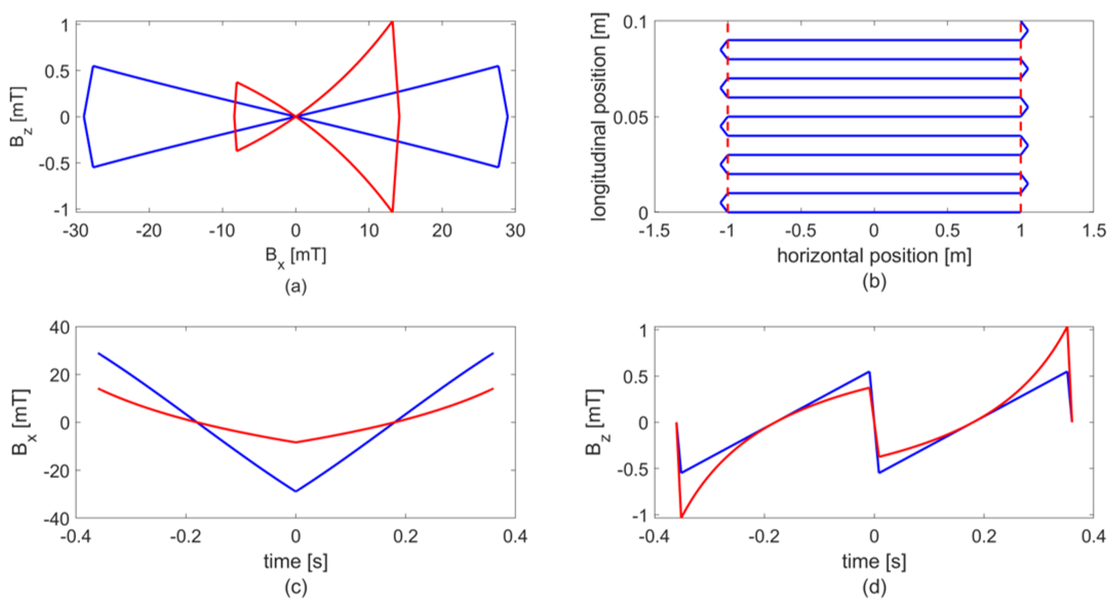
Based on the stated design parameters, Figure 4 shows the magnetic fields for the horizontal (x-direction) and longitudinal (z-direction) raster magnets in the rest frame and the resulting raster pattern as seen on the surface of the hide. In Figure 4b, the red lines represent the edge of the hide width, to show the overshoot region. Figure 4c,d shows $B_x$ and $B_z$ as a function of time. Note that for this particular choice of raster pattern, the longitudinal raster magnet oscillates at double the frequency of the horizontal raster. In doing so, the raster pattern in the rest frame forms a figure eight pattern, and this setup allowed us to minimise the range of movement in the longitudinal direction. We could, however, design a raster pattern that would appear as a triangle in the rest frame, but this would double the dynamic range for the longitudinal raster magnet.

2.4. Beam Loss in the Air

As the electron beam travels through the air, it will scatter with the air and lose energy, so this air gap must be minimized. Hence, a vacuum chamber was installed, as shown in Figure 1. Nevertheless, the beam travels through a 5–10 cm air gap before colliding with the hide. The beam energy loss due to the collision with air can be estimated by using the electron stopping power in the air. The stopping power of a material is the loss of energy per unit length. In our work, we considered a beam with 3–9 MeV energy, and their stopping powers in the air are given in

Table 2. Electron stopping power in dry air at sea level.

Beam Energy (MeV)	Stopping Power (MeV·cm${}^2$/g)	Energy Loss (MeV/cm)
3	1.783	2.18
4	1.850	2.27
5	1.911	2.34
6	1.967	2.41
7	2.020	2.47
8	2.068	2.53
9	2.115	2.59

[11]. The density of the dry air is 1.225 kg/m${}^3$ ($1.225\times$10${}^{-3}$ g/cm${}^3$), so the energy losses per centimetre are as shown in the third column. The electron beam will lose about 10–26 keV of energy depending on the beam energy (3–9 MeV) and air gap thickness (5–10 cm), which is insignificant as the beam energy is 2–3 orders of magnitude larger.

3. Simulation Studies

3.1. Irradiation and Energy Deposition

In this section, we present the simulation results where we studied the beam energy and beam delivery requirements in order to achieve a uniform depth dose distribution in the hide by using G4beamline [12], which is based on Geant4 [13]. Geant4 is a freely distributed toolkit under an open software licence and based on C++ using the Monte Carlo method for the simulating of particle interactions with matter. G4beamline simulates both accelerator beamlines and particle interactions with matter. The wet hides had an assumed density of approximately three times that of water and a thickness of around 8 mm. Therefore, in radiation deposition simulations, the hide was approximated/replaced by using water with a 2.5 cm depth.

3.1.1. Physics Model

The physics list used in our simulations was FTFP_BERT_LIV [14,15]. FTFP_BERT is the current Geant4 default and is good for most high-energy physics (HEP) processes. FTFP_BERT_LIV use a set of electromagnetic (EM) processes with the accurate simulation of gamma and charged particle transport by using the Livermore set of models. The default energy threshold limit of 990 eV was used. The physics processes included: photo-electric effect, Compton scattering, Rayleigh scattering, gamma conversion, ionization, and bremsstrahlung.

We can estimate the average distance travelled of photons in matter by using the equation:

$$\frac{I}{I_0}=e^{-\frac{\mu }{\rho }x},$$

(24)

where $I_0$ is the incident intensity, I is the intensity at mass thickness x and $\frac{\mu }{\rho }$ is the mass attenuation coefficient [16] of the target. The mass thickness is given by:

$$x=\rho t,$$

(25)

with $\rho$ being the density and t being the thickness of the material through which the X-ray travels. $\frac{\mu }{\rho }=4.078\times {10}^3$ cm${}^2/$g for the 1 keV X-rays in the water. The attenuation of 1 keV X-rays in the liquid water can be shown as in Figure 5. The intensity of the 1 keV X-rays is reduced to less than 2% in the 10 $\mathsf{\mu }$m of water, which indicates the error introduced by implementing a 1 keV cut-off energy in the simulation would be on the order of microns. Such an error was negligible as the water thickness in consideration in our study was four orders of magnitude larger. As the electrons interact more strongly than photons as they carry a charge, the error introduced by the electrons would be even smaller than that of the photons.

We also tested the Penelope set of models by using physics list FTFP_BERT_PEN [15]. They generated a similar depth-dose curve as shown in Figure 6, which closely resembles the results given in [17].

3.1.2. Double-Sided Irradiation

The energy deposited by the electron beam at a certain depth, known as the depth-dose curve or dose deposition curve, is energy dependent, as shown in Figure 7, where we considered the case where the hide was irradiated from one side (a) or both sides (b). The choice of single- or double-sided irradiation depends on several key factors, and throughout this section, we explore both possibilities.

We start by looking at double-sided irradiation as this requires a lower energy beam and has a higher energy efficiency than single-sided irradiation, as almost no radiation completely penetrates the entire thickness of the hide. However, assuming the hide density and thickness stated earlier, a beam energy below 2.5 MeV fails to penetrate to the central region of the hide, and for beam energies below 3.5 MeV, the peak dose deposition occurs before the central region.

In order to achieve a uniform dose distribution through the hide, beams with different dose deposition curves are required. This can be achieved in several ways, but the two methods we considered were where the beam energy is modulated (or the energy spectrum tailored) and where the angle of incidence is varied. As we shall see further on, varying the beam energy is qualitatively equivalent to varying the angle of incidence. We define the dose deviation, $D_d$, as the percentage variable in dose distribution along the depth of water:

$$D_d=\left(\frac{D}{D_{\mathrm{ave}}}-1\right)\times 100\%,$$

(26)

where D is the dose along the depth and $D_{\mathrm{ave}}$ the average of D. By using the dose deposition curves in Figure 7, we applied a least-squares algorithm to obtain the required energy spectrum of the beam, as shown in Figure 8a, which provided the uniform dose distribution shown in Figure 8b.

Unfortunately, the energy spectrum determined from the least-squares method was practically impossible to achieve. Due the the required dipole magnets to direct the beam, we expected that the maximum tolerable energy spread of the beam would be approximately 1%. An excessive energy spread would result in an energy modulation of the beam across the surface of the hide, which would impact the dose uniformity.

Figure 9 shows another solution, whereby rather than attempting to produce a complicated energy spectrum for a single-pass irradiation, we considered the possibility where the hide was irradiated over multiple passes, and on each pass, the beam energy and corresponding magnet strengths were varied to produce a relatively flat dose deposition curve (b) from a series of beams with different energies and intensities (a). This approach greatly simplified the setup, at the expense of requiring multiple passes of the electron beam. When operating the system in multi-pass mode, we would need to consider factors such as the raster magnet scanning rate, although this was not perceived to be a major issue as a raster frequency of ∼100 Hz was achievable and multi-pass irradiation would require a raster frequency of approximately 10 Hz. It should also be noted that this approach produced a better dose uniformity near the surface when compared to Figure 8.

3.1.3. Dependence on the Angle of Incidence

In the previous subsection, we noted that achieving a uniform dose distribution through the thickness of the hide would be practically impossible as a majority of the low-energy particles would be excessively scattered in the dipole magnets, and the generation of such a spectrum would not be possible with a single accelerator. Furthermore, it should be noted that for multi-pass operation, it would be extremely challenging to repeatedly produce beams below ∼1 MeV with a linear accelerator. Instead, this system would likely require a low-energy accelerator (>1 MeV) and a high-energy linear accelerator; which would likely drive up the cost of such a system. Another alternative is to consider a multi-pass system, where the angle of incidence of the beam onto the surface of the hide is varied on each pass; while maintaining a constant beam energy or requiring a much smaller range of energies. When electrons collide with the hide at an angle, more dose is deposited nearer the surface than for head-on irradiation; as shown in Figure 10. In this case, we assumed that the hide was irradiated from both sides to create a symmetric dose distribution pattern. This can be achieved by irradiating each side of the hide on separate passes. As a result, the effect of a non-zero angle of incidence was qualitatively similar to irradiating the hide with a lower energy beam, as can be seen in Figure 11. Here, we intentionally set the beam size to be infinitely small, so the angular spread was pronounced and clearly visible. However, the actual beam spot size on the hide would be larger and cover the whole surface of the hide, as addressed in the previous section.

As previously stated, we can combine dose deposition curves at different energies and different angles to generate a more uniform dose profile, as shown in the Figure 12, where we assumed that the hide was irradiated from both sides over a total of four passes. Figure 12a shows one example case where the dose deposition curves were added together for beams with different energies and angles of incidence (blue and black curves), and the combined dose distribution curve is shown in red. Figure 12b shows a comparison of the optimal dose deposition curve for different sets of parameters, where the beam energy and angle of incidence were varied. In the legend, $I_{x,y}$ represents the normalised intensity for a beam of energy, x MeV and an angle of incidence of $y^{\circ }$. In this plot, it should be noted that we limited the maximum angle of incidence to ${50}^{\circ }$. From Plot (b), it should be noted that the dose deposition curves were all similar, but the simplest configuration was the green curve because the beam energy remained constant and only the angle of incidence was varied.

The beam energy can be modulated in several ways. The simplest solution is to vary the linac accelerating gradient and dipole field strengths to achieve the required beam energies. Alternatively, another more complicated approach is to apply the beam energies in a single pass by extracting portions of the beam at different energies with the use of septum magnets [10]. The blue, black and green curves show the relative energy deposition from a series of mono-energy beams at indicated angles and beam energies. The red lines are the energy deposited by the mixture of these beams at the indicated mix ratios.

Large angles of incidence can be used to improve the dose uniformity near the surface, as shown in Figure 13. The large angle of 70${}^{\circ }$ deposited most of its energy near the surface; similar to the dose deposition from a low-energy beam. We can define the depth dose uniformity $U_{\mathrm{dd}}$ as:

$$U_{\mathrm{dd}}=\frac{D_{\max }-D_{\min }}{D_{\mathrm{ave}}},$$

(27)

where $D_{\max }$, $D_{\min }$ and $D_{\mathrm{ave}}$ are the maximum, minimum and average dose deposition, respectively. $U_{\mathrm{dd}}$ for Figure 13 is 8.6%. Another similar parameter we can use, which takes into account the actual beam distribution, is the normalised RMS dose deposition, ${\sigma }_{D_r}$, which is the ratio of the standard deviation of the depth dose, ${\sigma }_D$, and the average depth dose, ${\sigma }_{D_{\mathrm{ave}}}$, which can be written as:

$${\sigma }_{D_r}=\frac{{\sigma }_D}{D_{\mathrm{ave}}},$$

(28)

where for Figure 13, ${\sigma }_{D_r}$ = 1.7%.

3.1.4. Single-Sided Irradiation

In addition to irradiating the hides from both sides, we can consider a slightly simpler setup where the hides are irradiated from just one side. In doing so, we would need to use higher energy beams, and a significant portion of the beam energy would penetrate though the hide, reducing the energy efficiency of the entire process. The depth-dose curves are shown for the 6–10 MeV beams for an angle of incidence of $0^{\circ }$ (Figure 14). We see that the beam energy needs to be at least 8 MeV to achieve good dose deposition on the far side of the hide.

However, the key disadvantage with single-sided irradiation is that a significant portion of beam energy passed completely through the hide, resulting in a reduced energy efficiency when compared to double-sided irradiation. In order to improve the potential viability of this technology as a green tech alternative to conventional tanning, we aimed to maximise the irradiation efficiency, as this resulted in an increased wall plug efficiency and therefore lower overall energy consumption. The irradiation efficiency $\eta$ can be defined as:

$$\eta =\frac{P_{\mathrm{dep}}}{P_0},$$

(29)

where $P_{\mathrm{dep}}$ and $P_0$ are the deposited and incident beam power, respectively. As the beam energy increases, some of the electrons will penetrate though the 25 mm water, and the energy is not used for the tanning process. From Figure 14, the irradiation efficiencies for the 8 MeV and 9 MeV beams were 71% and 61%, respectively. This was much less compared to the double-sided irradiation’s 96.6% efficiency as summarized along with dose uniformity and average depth dose in

Table 3. Single- and two-sided slant irradiation results.

Irradiated Scheme	Double-Sided	Single-Sided	Single-Sided
Beam Energy (MeV)	3.5	8	9
$\eta$	96.6%	73.1%	64.6%
$U_{\mathrm{dd}}$	8.5%	7.7%	5.8%
${\sigma }_{D_r}$	1.6%	1.5%	1.1%

.

Figure 15 shows the dose deposition curves for an 8 MeV beam (a) and a 9 MeV beam (b), and the dose deviation is shown for the 8 MeV (c) and 9 MeV (d) beams, respectively. Qualitatively, these plots are similar, but the higher penetration from the 9 MeV beam improved the dose deposition on the far side of the hide.

Figure 16 shows the combined dose deviation curves from Figure 13 and Figure 15 to show a comparison between single- and double-sided irradiation. As we can see, both techniques had similarly flat dose depositions, but single-sided irradiation was slightly flatter and also required fewer passes to achieve a similar level of flatness.

Single-sided irradiation would require much higher beam energies than for double-sided irradiation. Furthermore, the reduced irradiation efficiency for single-sided irradiation means that a significant amount of dose was deposited in the conveyor system and supports, resulting in increased radiation and reducing the lifetime of the components. However, as we can see from the plots and table, single-sided irradiation improved the dose flatness, which in turn would improve tanning uniformity. The overall impact on the capital and running costs of the two systems, as well as the system complexity and reliability will be considered in future studies.

4. Conclusions

In this paper, we presented a design study for an electron accelerator in order to irradiate hides for a novel leather tanning process. As discussed in the Introduction, ensuring that we can achieve a uniform dose distribution throughout the volume of the hide is essential for effective tanning.

In Section 2, we presented a design study for a magnetic rastering scheme in order to scan the beam over the surface of the hide as it passed through the beam on a conveyor system, such that the surface dose distribution was uniform. We derived the differential equations that governed the rastering scheme and solved these with appropriate simplifications in order to determine the the rastering scheme. We also showed that we can successfully vary the angle of incidence of the beam, while still maintaining a uniform surface dose distribution.

In Section 3, we undertook dose deposition simulations using G4beamline in order to determine the energy spectrum of the beam required to achieve a uniform depth-dose curve. Initially, we considered a single pass, with zero angle of incidence (so the beam was perpendicular to the surface of the hide). In this case, we concluded that the energy spectrum would not be possible to achieve and that the lower energy particles would be lost by the deflecting magnets after the linac. We next considered a multi-pass system, where the beam was quasi-monoenergetic and a different beam energy was used on each pass, and we determined that this can produce acceptable dose uniformity. We then considered varying the angle of incidence instead of the beam energy and determined that this was qualitatively equivalent to varying the energy. We considered single- and double-sided irradiation and compared them in terms of irradiation efficiency, dose uniformity, tanning speed and shielding requirements. We found that double-sided irradiation had higher irradiation efficiency with just slightly less dose uniformity. Moreover, the double-sided irradiation required only 3.5 MeV, while double-sided irradiation needed 8–9 MeV. Therefore, the requirement for the shielding was much less for the double-sided irradiation, and hence, the cost is lower. However, it required flipping the hide, and hence more passes, as with lower energy, the dose rate was also low, so the tanning speed was lower. The single-sided irradiation had a much higher beam energy and hence higher dose rate and did not require flipping the hide, so it required fewer passes; therefore, it processed the hides much faster, but required much shielding. Both single- or double-sided irradiation have their pros and cons, but overall, double-sided irradiation is the better option to start with as it has much higher efficiency and requires much less shielding.

References

1. Brüning, O.S.; Collier, P.; Lebrun, P.; Myers, S.; Ostojic, R.; Poole, J.; Proudlock, P. LHC Design Report, CERN Yellow Reports: Monographs; CERN: Geneva, Switzerland, 2004; Available online: https://cds.cern.ch/record/782076 (accessed on 9 April 2021). [CrossRef]
2. Linssen, L.; Miyamoto, A.; Stanitzki, M.; Weerts, H. Physics and Detectors at CLIC: CLIC Conceptual Design Report. arXiv 2012, arXiv:1202.5940. [Google Scholar] [CrossRef]
3. Adolphsen, C. The International Linear Collider Technical Design Report—Volume 3. II: Accelerator Baseline Design, 2013, ILC-REPORT-2013-040. Available online: https://arxiv.org/abs/1306.6328 (accessed on 9 April 2021).
4. UNIDO’s Leather Panel, Case Study: Leather Industry Parks. 2017. Available online: https://leatherpanel.org/content/case-study-leather-industry-parks-planning-implementation-benefits-challenges-and-experience (accessed on 9 April 2021).
5. Mwinyihija, M. Ecotoxicological Diagnosis of the Tanning Industry. 2010. Available online: https://www.semanticscholar.org/paper/Ecotoxicological-Diagnosis-in-the-Tanning-Industry-Mwinyihija/3395884c77441d2641dc51b83fcd58fa40ee45ce (accessed on 9 April 2021). [CrossRef]
6. Blackman, A. Adoption of Clean Leather-Tanning Technologies in Mexico, 10881, Resources for the Future. 2005. Available online: https://ideas.repec.org/p/ags/rffdps/10881.html (accessed on 9 April 2021). [CrossRef]
7. RCRA in Focus—Leather Manufacturing, US Environmental Protection Agency. 2005. Available online: https://www.epa.gov/sites/production/files/2015-01/documents/k00002.pdf (accessed on 9 April 2021).
8. EU Legislation Regarding the Leather Industry. Available online: https://ec.europa.eu/growth/sectors/fashion/leather/legislation_en (accessed on 9 April 2021).
9. Lindgren, L.J.; Sandell, A.; Eriksson, M. Fast kicker magnet system. Nucl. Instrum. Methods Phys. Res. 1983, 214, 175–178. [Google Scholar] [CrossRef]
10. Barnes, M.J.; Borburgh, J.; Goddard, B.; Hourican, M. Injection and extraction magnets: Septa. In Proceedings of the CAS-CERN Accelerator School: Magnets, Bruges, Belgium, 16–25 June 2009; Brandt, D., Ed.; CERN-2010-004; CERN: Geneva, Switzerland, 2010. [Google Scholar] [CrossRef]
11. Berger, M.J.; Coursey, J.S.; Zucker, M.A.; Chang, J. Stopping-Power and Range Tables for Electrons, Protons, and Helium Ions; NIST Standard Reference Database 124; National Institute of Standard and Technology: Gaithersburg, MD, USA, July 2017. [Google Scholar] [CrossRef]
12. G4beamline Release 3.06 is available (January 2019). Available online: http://www.muonsinternal.com/muons3/G4beamline (accessed on 9 April 2021).
13. Agostinelli, S. Geant4—A Simulation Toolkit. Nucl. Instrum. Methods Phys. Res. 2003, 506, 250–303. [Google Scholar] [CrossRef] [Green Version]
14. Geant4 Collaboration. Geant4 Physics Reference Manual; Release 10.7; Rev5.0; CERN: Geneva, Switzerland, 4 December 2020. [Google Scholar]
15. Allison, J.; Amako, K.; Apostolakis, J.; Arce, P.; Asai, M.; Aso, T.; Bagli, E.; Bagulya, A.; Banerjee, S.; Barrand, G.; et al. Recent developments in Geant4. Nucl. Instruments Methods Phys. Res. Sect. A Accel. Spectrometers Detect. Assoc. Equip. 2016, 835, 186–225. [Google Scholar] [CrossRef]
16. X-Ray Mass Attenuation Coefficients; NIST Standard Reference Database 126; National Institute of Standard and Technology: Gaithersburg, MD, USA, July 2004. [CrossRef]
17. International Organization for Standardization. ISO/ASTM 51649:2002 Standard Practice for Dosimetry in an Electron Beam Facility for Radiation Processing at Energies Between 300 keV and 25 MeV; ISO: Geneva, Switzerland, 2002. [Google Scholar]
Figure 1. Irradiation system layout. It should be noted that the hide and conveyor system are in air, and the beam passes through a vacuum window to transition from the vacuum to the air gap.
Physics 03 00017 g001
Figure 2. Schematic diagram showing the geometry of the beam trajectory through the raster scanning magnet to the hide. θ is the deflecting angle of the magnet, ρ is the radius of curvature, δ l is the apparent turning point of the beam from the end of the magnet when modelling the magnet as an instantaneous impulse, L dip is the length of the dipole magnet and L drift is the length of the drift section after the dipole magnet.
Physics 03 00017 g002
Figure 3. Hide orientation for an angle of incidence of (a) 70 and (b) 0 . The blue lines represent the trajectories of the electron beam at different deflection angles in the x-y plane, the red curves represent the surface of the hide, the black lines are the normals to the hide and the green regions in (a) is to show that the angle between the beam and the normal to the hide is constant regardless of beam deflection angle.
Physics 03 00017 g003
Figure 4. Raster pattern for an angle of incidence of 0 (blue) and 70 (red) in (a) the rest frame, the projected raster pattern on the surface of (b) the hide and (c) B x and (d) B z vs. time. In (b), the raster pattern projected on the surface of the hide is the same for all angles of incidence. The dashed red lines represent the edge of the hide to highlight the overshoot regions.
Physics 03 00017 g004
Figure 5. Attenuation of the 1 keV X-ray in liquid water.
Physics 03 00017 g005
Figure 6. Depth-dose curves generated by different energies of electrons in water in the simulation by using the (a) Livermore and (b) Penelope set of models.
Physics 03 00017 g006
Figure 7. Energy deposition vs. water depth for different beam energies when irradiated from (a) one side and (b) both sides for an angle of incidence of 0 .
Physics 03 00017 g007
Figure 8. (a) The kinetic energy (KE) spectrum and (b) the dose deviation, obtained by a least-squares method to provide a uniform depth-dose curve.
Physics 03 00017 g008
Figure 9. (a) The kineetic energy (KE) spectrum for multi-pass, multi-energy irradiation of (b) the hide and the resulting dose deviation. The spectrum is obtained by using the least-squares algorithm and limiting the combination to five mono-energetic beams.
Physics 03 00017 g009
Figure 10. Irradiation with 3.5 MeV at (a) 0 and (b) 45 angle beams. The red/green lines are the trajectories of electrons/photons. The grey colour is 2.5 cm thick (from left to right) water.
Physics 03 00017 g010
Figure 11. Depth-dose curves for a 3.5 MeV beam with a varying angle of incidence.
Physics 03 00017 g011
Figure 12. (a) Combined depth-dose curves for a 3.5 MeV beam with an angle of incidence of 50 and a 3.6 MeV beam with an angle of incidence of 0 , and (b) a comparison of the dose deposition curves for different combinations of beam energy and angles of incidence. I is the beam intensity as given in Equation (24).
Physics 03 00017 g012
Figure 13. (a) Dose deposition curves for different angles of incidence, and (b) the corresponding dose deviation of a 3.5 MeV beam. I is the beam intensity as given in Equation (24).
Physics 03 00017 g013
Figure 14. Single-sided irradiation with high-energy beams. η is the irradiation efficiency as defined in Equation (29).
Physics 03 00017 g014
Figure 15. Single-sided irradiation by combining beams with different angles of incidence for (a) 8 MeV and (b) 9 MeV beams. Dose deviation for (c) 8 MeV and (d) 9 MeV beams. I is the beam intensity as given in Equation (24).
Physics 03 00017 g015
Figure 16. Comparison of dose deviation of single- and double-sided irradiation. I is the intensity as given in Equation (24).
Physics 03 00017 g016