A Perspective on the Solar Modulation of Cosmic Anti-Matter


1
Institute for Experimental and Applied Physics, Christian-Albrechts University in Kiel, 24118 Kiel, Germany
2
Centre for Space Research, North-West University, Potchefstroom 2520, South Africa
3
School of Physical and Chemical Sciences, North-West University, Mmabatho 2735, South Africa
*
Author to whom correspondence should be addressed.
Physics 2021, 3(4), 1190-1225; https://0-doi-org.brum.beds.ac.uk/10.3390/physics3040076
Submission received: 1 October 2021
/
Revised: 19 November 2021
/
Accepted: 19 November 2021
/
Published: 7 December 2021
(This article belongs to the Special Issue A Themed Issue in Honor of Professor Reinhard Schlickeiser on the Occasion of His 70th Birthday)
Abstract
:Global modulation studies with comprehensive numerical models contribute meaningfully to the refinement of very local interstellar spectra (VLISs) for cosmic rays. Modulation of positrons and anti-protons are investigated to establish how the ratio of their intensity, and with respect to electrons and protons, are changing with solar activity. This includes the polarity reversal of the solar magnetic field which creates a 22-year modulation cycle. Modeling illustrates how they are modulated over time and the particle drift they experience which is significant at lower kinetic energy. The VLIS for anti-protons has a peculiar spectral shape in contrast to protons so that the total modulation of anti-protons is awkwardly different to that for protons. We find that the proton-to-anti-proton ratio between 1–2 GeV may change by a factor of 1.5 over a solar cycle and that the intensity for anti-protons may decrease by a factor of ~2 at 100 MeV during this cycle. A composition is presented of VLIS for protons, deuteron, helium isotopes, electrons, and particularly for positrons and anti-protons. Gaining knowledge of their respective 11 and 22 year modulation is useful to interpret observations of low-energy anti-nuclei at the Earth as tests of dark matter annihilation.
1. Introduction
Galactic anti-matter, specifically positrons and anti-protons, has been observed on Earth simultaneously, continuously and with high precision over prolonged periods of time by PAMELA [1,2,3] and AMS-02 [4,5]. Although these missions, deployed in geospace, were designed to study specific astrophysical characteristics related to galactic cosmic rays (GCRs), they both have contributed extensively to the study of solar modulation in the inner heliosphere. For solar modulation and numerical modelling studies, observations of GCRs lower than ~30 GV are essential, with modulation effects growing in significance the lower the rigidity is. In this context, PAMELA had recorded GCRs down to ~80 MV from 2006 to 2016, ending just after the recent maximum solar activity. AMS-02 has been recording GCRs down to ~0.5–1.0 GV since 2011, including the period of solar maximum activity, the reversal of the heliospheric magnetic field (HMF) and the recent solar minimum period with published spectra averaged over Bartels rotations until 2017. However, full spectra of anti-matter particles detected at regular intervals (e.g., every solar rotation) by these missions have not been published. This lower limit in energy of AMS-02 is not ideal for studying the exceptional features of solar modulation occurring at lower energy but the consistent preciseness of these observations over time has opened up other avenues that can be studied in conjunction with sophisticated numerical models. These recurrently measured spectra of such a variety of GCRs over an extensive period of time have made it possible to take also the investigation of the modulation of GCRs with comprehensive numerical models to a higher level of preciseness at a rigidity range not previously achievable. This encourages studying modulation effects occurring at Earth that are quite small and which on its part provides interesting challenges to numerical modeling attempting to explain these easily overlooked features and the underlying physics on which they are based.
Observations of GCRs made by the two Voyager spacecraft in the outer heliosphere have been of utmost importance for modeling efforts on a global scale. Voyager 1 and 2 crossed the heliopause (HP) in August 2012 at 121.6 AU and in November 2018 at 119 AU from the Sun, respectively, but far apart, about 167 AU, and at different heliographic latitudes [6,7]. It is now reasonably well known how wide the inner heliosheath is, what the average distance is between the termination shock (TS) and the HP and where the HP is located as the preferred modulation boundary (at least in the nose-direction of the heliosphere). Also, that none or very little modulation of GCRs (e.g., [8,9,10]) seems to occur beyond the HP (this region is considered to be the outer heliosheath, depending on the shape of the heliosphere and given that a heliospheric bow shock may exist; see [11,12]. Since no significant GCR spatial gradients in intensity were observed over this vast outer heliospheric region, the assumption that the local interstellar spectra (LISs) for GCRs are arriving isotropically at the heliosphere still seems reasonable (except at very high rigidity where it is less than 0.1% (e.g., [13,14]). The point is that three-dimensional (3D) simulations can now be done much less speculatively than before, both in terms of the spatial dimensions of the heliosphere and what spectra to utilize at the modulation boundary as very LISs (VLISs), an aspect that will be discussed in depth in the next section. It is fair to say that the global and total modulation of GCRs between the HP and the Earth can be described and simulated more convincingly than before. In this context a number of open publications by the late W.R. Webber and his colleagues can be found on the eprint archive arXiv. Also important to the aspired enhancement of global numerical modelling are observations that were made by the Ulysses mission in the inner heliosphere between 1990 and 2009 from which an interpretation could be formed of how GCR modulation may happen at high heliolatitudes (e.g., [15,16]; and the reviews in [17,18]).
In the context of establishing VLISs, both Voyager spacecraft have made measurements in the kinetic energy (KE) range of 3 MeV/nuc to 346 MeV/nuc for protons, total helium and other light GCR nuclei as well as for electrons (actually negatrons) from 2.7 to 74 MeV [19]. The energy range for these particles was specified somewhat differently in [20,21] also reported observations for the secondary GCR isotopes H-2 (2H1 deuteron), and He-3 (3He2), apart from protons and He-4 (4He2), as primary particles. However, anti-matter such as positrons and anti-protons are not measured by them, so that it remains an issue what to use at these low rigidities for their VLISs in global modeling. Fortunately, solar modulation can be considered negligible at an appropriate high enough rigidity where precise measurements now exist so that at least their VLISs are easily determined at these high rigidity values. The only point of contention here is at what rigidity the solar modulation of GCRs truly commences [22].
A way to test for dark matter annihilation may be found in observations of low-energy anti-nuclei in GCRs, such as anti-protons, anti-deuteron and anti-helium, making the proper numerical study of the modulation of these anti-particles in the heliosphere imminent. Rudimentary modulation models, such as the Force-Field model [23] and analytical variations there-of (e.g., [24]), are inadequate for this purpose and can easily yield misleading results when it comes to precise modeling as pointed out in [25,26,27,28].
The layout of this paper is as follows: First the essence of the basic transport theory used for numerical models and our modeling approach to solar modulation studies are briefly described, including global modulation parameters, as well as the diffusion coefficients in terms of their rigidity dependence. Particle drifts are discussed and what the drift related predictions for solar modulation are and how it manifests from the difference between the modulation of electrons and positrons, protons and anti-protons and what differences there are between positrons and anti-protons. In Section 3, the manner is discussed in which the relevant VLISs are established by using both observations and numerical modulation models. In Section 4 and Section 5 simulations of the modulation of positrons and anti-protons are shown in particular and the differences between them are discussed. A brief discussion is given on the modulation of other types of anti-matter, with a summary and a compilation of computed VLISs in the conclusion.
2. Numerical Model and Modeling Approach to Solar Modulation Studies
2.1. Theory and Assumptions
The modeling here is based on solving numerically the transport equation (TPE) derived in [29]:
where is the omnidirectional GCR distribution function, p is particle momentum, r is the heliocentric position vector and t is time. The differential intensity of GCRs is given by I = p2f or equivalently I = R2f, where R is rigidity in GV. The terms on the right-hand side represent diffusion, convection, gradient and curvature drifts, and adiabatic energy changes. The solar wind velocity is . Adiabatic energy losses occur when which applies to most of the heliosphere. The diffusion tensor K consists of three distinct diffusion coefficients (DCs), first, which is parallel to the average HMF, which is radially perpendicular to this field and which is perpendicular to this field in the heliospheric polar direction. The averaged guiding center drift velocity for a near isotropic distribution is given by
with . Here, is the drift coefficient (in the literature it is also indicated with ) where B is the magnitude of the background HMF at a given position in the heliosphere, the value of which changes spatially and with solar activity.
The global HMF is assumed to have a basic Parkerian geometry in the equatorial plane, but modified in the polar regions similar to the approach of [30]; for a full description of this particular aspect, see [31]. The global latitudinal dependence of the V is assumed to change from 430 km s−1 in the equatorial plane to 750 km s−1 in the polar regions only during solar minimum activity in accordance with Ulysses observations (see [32], and reference there-in; and reviews [17,18,33]). The HP position is assumed at 122 AU, with any asymmetry in the shape of the heliosphere considered to be negligible for GCR modulation studies (e.g., [34,35]). The position of TS is changed according to solar activity levels [36] from 88 AU (e.g., in 2006) to 80 AU (e.g., in 2009). The shock compression ratio of 2.5 is assumed for the TS consistent with observations [37,38] in order to account for the drop in V beyond the TS as assumed in the model. For details on this modeling approach, see [39] and references there-in. However, the re-acceleration of GCRs at the TS is not considered for this study; for details on such a modeling approach; see [40,41].
This 3D numerical model and all relevant assumptions were comprehensively described in [42,43,44,45,46]. The main features of this model and several applications can also be found in these publications as well as those recently published [47,48,49,50,51]. For general reviews on solar modulation, see [27,33,52,53,54] and for reviews on deriving transport equations for GCRs, see [26,55,56] for those applicable to heliospheric transport.
2.2. Modeling Approach
The method and procedures followed here consist of the following: The VLIS for electrons and protons were established as the first step and then used in the 3D modulation model to reproduce the observed electron and proton spectra at the Earth from PAMELA for 2006 to 2009, thus focussing at first on solar minimum conditions. This was extended to include both PAMELA and AMS-02 spectra for after solar minimum to full maximum conditions, including the reversal of the HMF polarity during solar maximum and afterwards up to the present solar minimum. In this manner the model, with its assumptions about the global heliosphere as well as all the modulation parameters, DCs and the drift coefficient were tested and vindicated. The set of proton modulation parameters was applied to other GCR nuclei, e.g., helium isotopes as well as anti-protons over time (solar activity) and the electron parameter set was applied to positron modulation. This assures that the modeling parameters are not changed in an ad hoc and inconsistent manner for the purpose of simply fitting observational data sets at the Earth, including those for GCR anti-matter.
The only differences in the modulation of protons and anti-protons are their global drift directions in the heliosphere, and of course, their VLISs; similarly the only differences in the modulation of electrons and positrons are their VLISs and their global drift directions. The latter is of course responsible for the charge-sign dependent modulation effect over a 22-year cycle related to the reversal of the HMF polarity as will be discussed further in what follows.
Reproducing the precise observational spectra on Earth, especially at higher R, is being studied to determine refinements to the rigidity dependence of the DCs over time. This approach allows that the mentioned three DCs and the drift coefficient can be quantified in terms of their rigidity so that the ‘free parameter space’ in these models has become significantly reduced. How the 11-year and specifically the 22-year modulation cycles come about are explained, including charge-sign effects, the physics of which is not described by the Force-Field modulation approach (e.g., [27,57,58,59]).
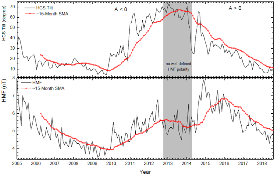
The 3D numerical model for this modulation study is for a steady-state, so that in Equation (1), so that modulation effects shorter than 27-days and all transient events such as Forbush decreases or co-rotating interaction regions cannot be adequately described with this model. Determination of the averaged values for modulation parameters that vary with solar activity is an important part of the modeling approach, specifically the tilt angle α of the heliospheric current sheet (HCS) and the magnitude B of the HMF, both considered as good proxies for solar activity when it comes to charged particles; see also [60,61]. These variations in α and B are used in the numerical model to set up realistic modulation conditions for each epoch.
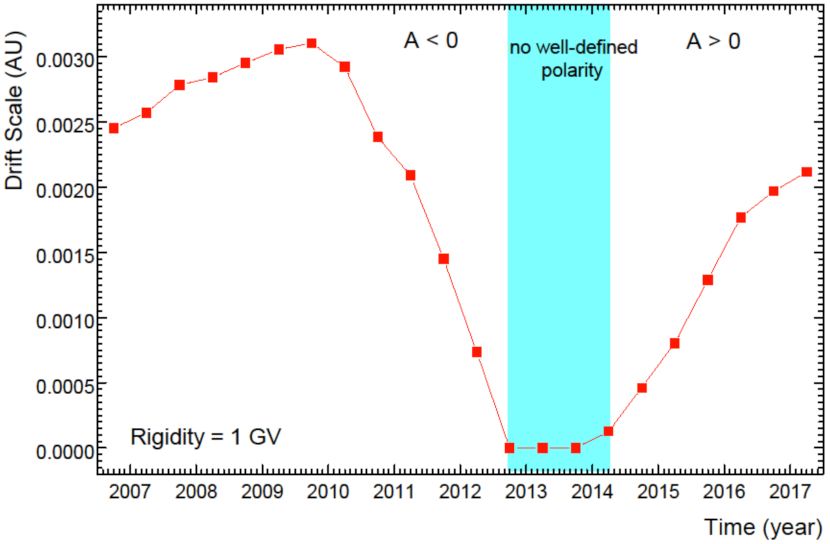
The top panel of Figure 1 shows α at Earth from 2005 to 2018 [62] together with the calculated 15-month smoothed moving averages (SMAs) as used in the model. The observed B values at the Earth are shown in the bottom panel for the same period [63] together with the corresponding SMA. Also shown in this figure is the period when no well-defined HMF polarity was reported, as indicated by the shaded band, and during which the HMF polarity reversal occurred [64]. There seems no consensus on the exact time span of this band as discussed in [65]. However, important is that before this period the polarity of the HMF was A < 0 and afterwards A > 0; see the detailed discussion in Section 2.5.1. The lowest values of both α and B occurred in 2009 as part of that prolonged solar minimum, of which the specific modulation effects were discussed in detail in [42]. It is expected that similar low values may occur during the present solar minimum period. The highest values for α occurred around the beginning of 2013, with extraordinary high but temporary values in 2011 and late in 2014, but for B the highest values occurred in late 2014, remaining relatively high until the end of 2015.
2.3. Rigidity Dependence of the Diffusion Coefficients
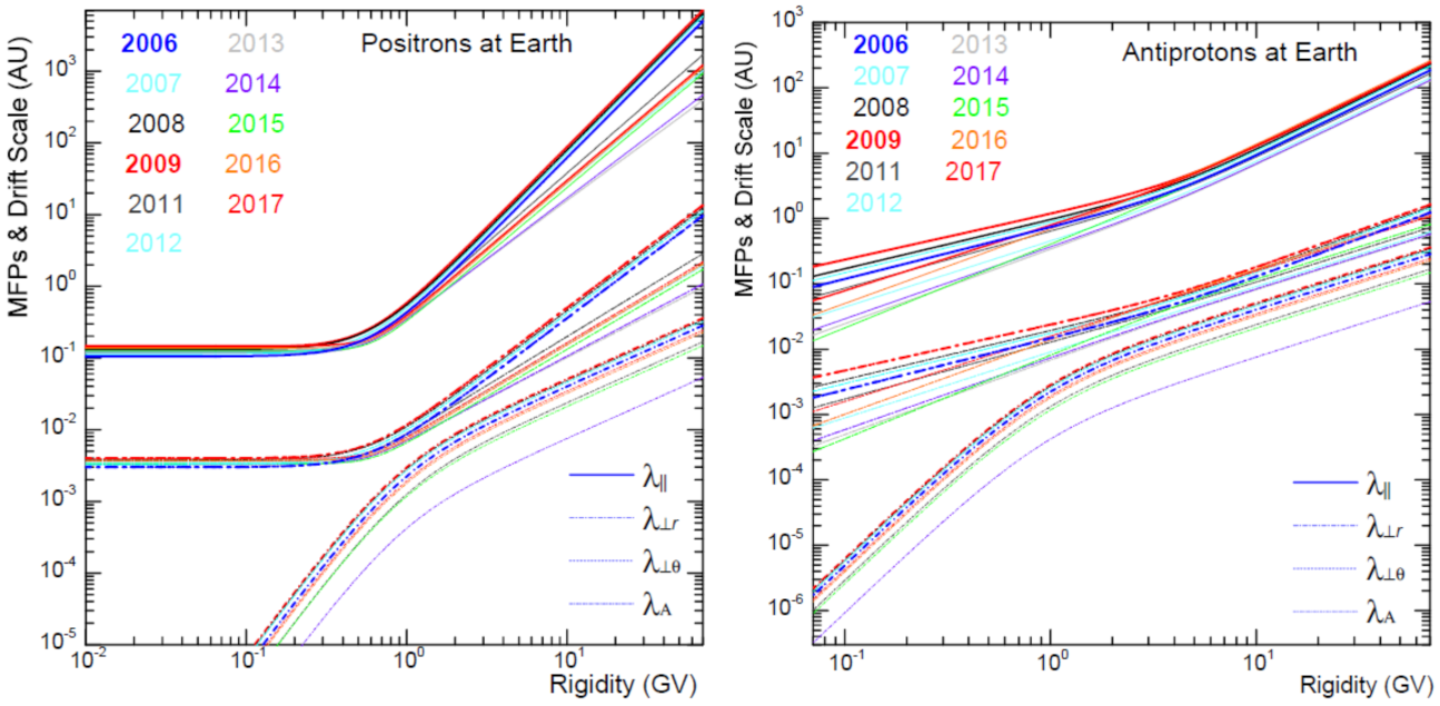
The DCs for GCR modulation in the heliosphere are related to the particles’ mean free paths (MFPs), λ, through with v = βc the particle’s speed, c the speed of light so that β is the corresponding ratio. The relationship between, e.g., and is given then by , similarly for and . The rigidity dependence of the three relevant MFPs and the drift scale are shown in Figure 2 for positrons in the left panel and for anti-protons in the right panel for yearly averages from 2006 to 2017 as established in [45,60,66,67] in order to reproduce the corresponding observed electron and positron spectra, and the proton and anti-proton spectra at Earth.
Figure 2 illustrates important aspects of how positrons and anti-protons (and electrons and protons) in terms of the R dependence of their MFPs are modulated, apart from the depicted time-dependence which is discussed later. Both these particle types have a different R dependence for the three MFPs at low compared to high R; for positrons this change in spectral slope occurs typically around ~0.4 GV and for anti-protons around ~4 GV, with steeper slopes consistently above these turn-point (tipping point) in R. The R-dependence of and are the same and modestly different from at high R but not at low R; overall and are only about 2% of the value of but their values differ away from the equatorial plane of the simulated heliosphere (see [45]). The MFPs for positrons (and electrons) have a characteristic slope, almost independent of R below ~0.4 GV, which means that the total value of the modulation of these particles between the HP and the Earth is the same below 0.4 GV because their modulation is diffusion-dominated in this rigidity range, not adiabatically-dominated as for protons and anti-protons. This aspect was elaborately illustrated with GCR spectra [45,60,66,67] and relates to what was discussed theoretically in [68,69,70] and from a turbulence theory point of view in [55,71]. The drift scale also shows a difference at high R (where ) compared to low R, with the change in spectral slope occurring typically between 1–2 GV for both positrons and anti-protons. This significantly steeper decrease in for R < ~1 GV has been reported and studied comprehensively with numerical models (e.g., [72], and references there-in) and theoretically (e.g., [73,74], and references there-in).
In the modeling used here it is assumed that the DCs (and MFPs) in terms of their spatial dependence scale proportional to with = 1 nT. This is the simplest and most pragmatic approximation to turbulence theory that can be assumed for DCs in numerical models and has turned out to be quite reasonable; for discussions and applications of more complicated assumptions regarding the relationship between these DCs and heliospheric turbulence; see [72,75,76,77,78]. Mathematical expressions for the R-dependence of the three MFPs, and the drift scale, as shown in Figure 2, are not repeated here (they are quite lengthy and would take up a substantial amount of space). They were given extensively in [48,60,72], and many were also utilized in [47,79,80,81].
2.4. Time Dependence of the Diffusion Coefficients
Another intriguing aspect of what is depicted in Figure 2 is the time variation found for the R dependence of the MFPs. For anti-protons their time variation is largest below 4 GV with a remarkable spread in values between 2006 and 2017, at the lowest R this spread is in the order of a factor of 10 but much less above 4 GV, about a factor of 3. This is a manifestation of the larger modulation that GCRs nuclei experience the lower the rigidity. For positrons (and electrons) this is different; the spread in time is significant for R > 0.4 GV, in the order of a factor of 10 but less significant below this value. The latter is based on comparing the model with published PAMELA observations for the solar minimum period before 2010; for electrons the observational cut off was established at ~80 MeV but originally higher for positrons at ~200 MeV because of statistics [2,82]; with AMS-02 observations from R > 0.5 GV but usually published for R ≥ 1 GV ([5] and references there-in). This aspect, as well as the apparent steady behaviour in terms of rigidity, is therefore difficult to investigate more precisely, also complicated by Jovian electrons that dominate the spectrum at the Earth below ~50 MeV [83,84]. Although observations (detection) of electrons and positrons at lower R in geospace are intricate [85,86], such data will be quite useful for future analysis. For this time dependence is about the same at all rigidities, although somewhat less for R < ~1 GV than above; see also [81].
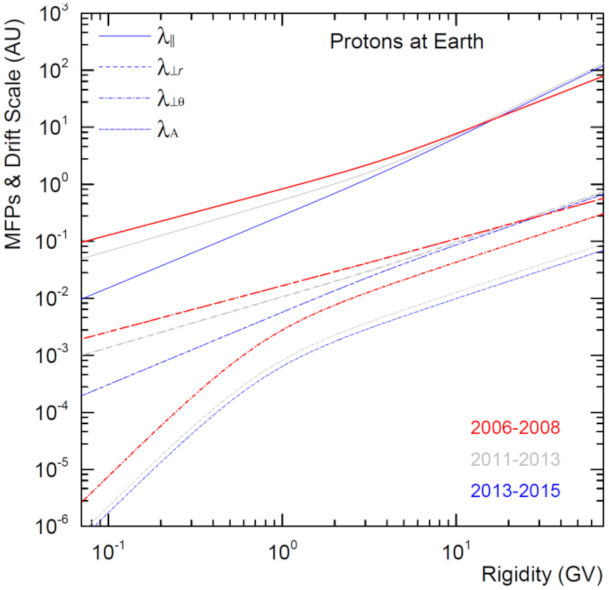
Emphasizing the significance of the mentioned time dependence, Figure 3 shows , and as determined for protons (assumed to be valid also for anti-protons) but now averaged over three distinct periods, for solar minimum conditions from 2006 to 2008, for increasing solar activity from 2011 to 2013 and then for maximum activity conditions from 2013 to 2015, in order to reproduce both PAMELA and AMS02 proton and antiproton spectra. Qualitatively, similar behaviour is shown as in Figure 2 but now it clearly illustrates how the time dependence differ below and above ~10 GV; below this value the MFPs decrease progressively and significantly from 2006–08 to 2013–15 but the opposite, and at a much smaller scale, occurs above this value. This seems counterintuitive, but similar behaviour (trends) using precise spectra from AMS-02, was reported also in [80,81,87] and implies that GCRs with R > 10 GV have somewhat smaller MFPs at solar minimum than at solar maximum; as such quite an interesting aspect of solar modulation at higher rigidity. In this context, it is well known that time trends in modulation is occurring differently at low and high rigidity during A > 0 and A < 0 cycles; see the discussion in [88,89], and references there-in, and recent modeling studies (e.g., [81]).
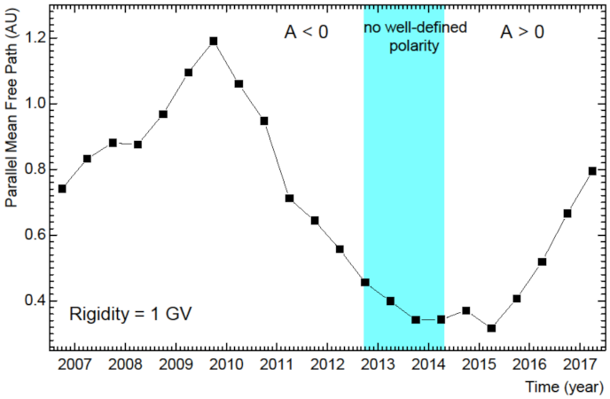
An example of the time dependence of at the Earth is shown in Figure 4 for protons and anti-protons at 1 GV from July 2006 to May 2017. The period with no well-defined HMF polarity is indicated again by the shaded band, during which the HMF polarity changed from A < 0 to A > 0. During the A > 0 solar minimum had reached a maximum value in late 2009 and then decreased systematically to reach a minimum value in early 2015, apparently several months after the reversal of the HMF polarity was completed. The value in 2017 is already close to that in 2006 which was the beginning of the previous prolonged solar minimum. This investigation will be continued when new AMS-02 spectra get published for the present solar minimum (before and after 2020). A similar time-dependence was found for positrons and electrons in [62] with qualitative similar results.
2.5. Particle Drifts in the Heliosphere
As alluded to above, the solar modulation effects on GCRs of global gradient and curvature drifts, including the effect of the wavy HCS, are known and reported extensively since its introduction [90] and first modelled in 3D [91]. The main predictions are mentioned in the next section. Global particle drifts is one of the four main modulation processes as described in Equation (1). As numerical models have become more sophisticated, including the stochastic differential equation (SDE) approach to modulation modeling [9,31,92,93] and as new long-term and precise observations have become available from time to time, the insight on how large drift effects are and how this may change with rigidity, with space and with solar activity, as well as from one 11-year cycle to the next one, has significantly improved since the 1980’s.
It has been realized that what is known theoretically as weak-scattering drift is an oversimplification. This is obtained by assuming that in the heliosphere , where is the gyro-frequency of a charged particle in the HMF as a given location and with τ a time scale defined by its scattering so that the drift coefficient simplifies to:
This expression was used in earlier numerical models and obviously has an uncomplicated rigidity dependence, with its spatial dependence determined by what is assumed for B. During the Ulysses mission it became evident that this gives a far too large drift effect concerning the observed GCR latitudinal intensity gradients [17,33,39,54] at low rigidity, typically at R < 1 GV. This mission also indicated that Parker’s descriptions of the global HMF structure is an oversimplification [94]. Nowadays, it is common practice in numerical modeling to modify KD at lower rigidities as shown in Figure 2 and Figure 3, and to modify the global geometry of the HMF to some degree; see [35,48,72] for the appropriate expressions and [31,94] for a study on HMF and HCS modifications. An extensive theoretical study on the reduction of particle drift, using various assumptions for heliospheric turbulence, was described in [74] (and references there-in) with previous related studies in, e.g., [73].
Apart from these explicit reductions of particle drift, the more subtle reduction of drift related modulation effects is done through changing diffusion which follows from the inspection of Equation (1) according to which the drift velocity is multiplied by (in effect the spatial gradients of the GCR intensity in the heliosphere at a given position and KE). This means that when these gradients are changed through changing any of the three DCs, drift effects consequently change. This is considered an implicit reduction of drift effects, not directly affecting the drift coefficient In this context, what is assumed, for example, for is quite important because it affects directly the intensity gradients in the polar regions of the heliosphere and therefore the corresponding drift related modulation effects see also [72,84].
Another aspect of interest is how drift effects change with solar activity. At first, these effects were changed in simulation studies only through changing the waviness (tilt angles) of the HCS and later followed by changing B as it changes with solar activity. These aspects were simulated comprehensively in [95,96,97] who also introduced the concept of global merged interaction regions (GMIRs) into drift modeling; for more recent such simulations, see also, e.g., [98,99]. Simulations of these GMIRs showed that they could easily dominate the level of GCR modulation depending on how extensive in space they are and how many of them form beyond 5–10 AU during phases of higher solar activity. Particle drifts appeared to be dominant during solar minimum epochs (see review [100]) but how much particle drifts remains during periods of high solar activity could not be answered conclusively. However, afterwards it became clear that (or ) is required to be scaled with time in order to reproduce GCR observations over extended periods of time, specifically from the Ulysses mission; see reviews [17,18,33]. Examples of numerical simulation utilizing such an approach were given in [34,101,102,103] who also studied other modulation effects such as the role of the TS and inner heliosheath. Later, [104,105] applied a time-dependent scaling factor in their numerical model to reproduce GCRs at the Earth and especially along the trajectories of the two Voyager spacecraft. The first numerical calculations on specifically how KD scales (effectively being reduced) over periods of increased solar activity up to solar maximum conditions was given in [106] when comparing their simulations to Ulysses observations. They found that relatively little particle drift (<10%) remained during the solar maximum periods of 1990–91 and 2000–02. Recently, [45,62] determined how much particle drift is needed at 1 GV to explain the time dependence from 2006 to 2015 related to the observed precise electron and positron spectra from PAMELA and AMS-02 during each solar activity phase, especially during the polarity reversal phase when no well-defined HMF polarity was present. The equivalent result based on our simulations of proton and anti-proton modulation is shown in Figure 5. Evidently, very little drift is found and required for the period of maximum solar activity.
2.5.1. Drift Related Modulation Effects
A main feature of drift related modulation is that the particle drift velocity field repeats its configuration every 22 years because it changes direction when the solar magnetic field flips over during every period of maximum solar activity. The northern and southern polar field then reverses sign so that if the direction in the northern hemisphere had been outwards it became inwards after the reversal. This process is known as the ‘polarity’ change of the solar magnetic field. The time it takes for the reversal to be completed differs from one solar maximum to the next one and how the process happens in time is always different for the northern polar field than for the southern field; see, e.g., [64]. From the view point of charged-particle drifts and solar modulation, the important aspect is that this period is characterized as a time with no well-defined HMF polarity and that it usually lasts more than a year. To briefly recap: The drift cycles are called A < 0 (e.g., 2001–2012) when positively charged GCRs (protons, positrons, GCR nuclei.) drift inward to the inner heliosphere mainly through the equatorial regions of the heliosphere, and in the process encounter the wavy HCS, and outward via the polar regions of the heliosphere. Negatively charged particles (electrons, anti-protons, anti-matter nuclei) then drift inwards and downwards to the Earth mostly from the polar regions and then outward mainly through the equatorial regions. During an A < 0 phase, it is expected that the changing wavy HCS plays an important even dominant role in the modulation of positively charged particles, whereas for an A > 0 polarity phase the drift directions become reversed so that negatively charged particles encounter the HCS during their entry.
The consequence of what is described above is that it produces a 22-year modulation cycle, not just in the GCR intensity-time profiles but also spatially in terms of the distribution of the radial and latitudinal intensity profiles in the heliosphere (and consequently the spatial gradients), and with the charge-sign dependent effect probably the most spectacular. Illustrative examples of the observation of this phenomenon with the Ulysses mission [15,107] and subsequent modeling was given in [108]. A full list of these drift related phenomena were given in the review [59].
A very subtle drift effect, not always mentioned, is the prediction that proton spectra for A < 0 solar minimum cycles compared to A > 0 minimum cycles should exhibit a spectral cross-over with means that below this cross-over rigidity the differential intensity is higher in the A > 0 than in the A < 0 cycles but not above this rigidity [109,110,111], as long as solar activity is at the same level. This phenomenon is discussed in detail in [88,89], especially how it is predicted with precise numerical modeling and how difficult it is to find and confirm observationally but surely possible now that precise long-term spectral observations have become available.
During the prolonged solar minimum before 2010, PAMELA had observed and confirmed the charge-sign dependent effect between electrons and protons conclusively [112] and later reported how this effect for electrons and positrons had changed with the reversal of the HMF polarity [2,113], although smaller than predicted by the leading drift models of that time [59]. Such an effect was also found for the very first time in the recover times of observed proton and electron Forbush decreases [114] and comprehensively modelled by [115]. The charge-sign dependent effect during the recent HMF polarity reversal was also observed and reported by AMS-02 [5], confirming the PAMELA observations, and is discussed further in Section 4 and Section 5 comparison with our drift modeling.
3. The Question of VLISs at the Heliopause
The VLISs for GCRs are required as input spectra for the numerical modelling of their total and global modulation in the heliosphere [46,116,117,118,119,120,121]. For each type of charged cosmic particles such a specific input spectrum is considered to be unmodulated by solar activity beyond the HP. Global modulation modelling relates these VLISs to the corresponding observations at the Earth, through the physics contained in the assumed transport model applicable to the heliosphere. In order to reproduce (simulate) observed spectra over a wide rigidity range at the Earth for any type of GCRs, their associated VLISs must first be determined and evaluated against galactic propagation models such as GALPROP (e.g., [121,122,123]) and then tested and vindicated with comprehensive 3D modulation models as described here.
After Voyager 1 had observed GCRs at and beyond the HP, the question came up whether these spectra at ~122 AU, technically just heliopause spectra, could be used as VLISs and if the latter are truly the same as pristine LIS (say, 1000 AU away from the Sun) and if they were on their part truly the same as the averaged Galactic spectra (parsecs away). These questions have led to predictions done with SDE type modulation models that GCRs may be modulated even beyond the HP implying that the heliopause spectra were not the same as LISs and that the HP should not be considered the true modulation boundary. The original prediction [124] had come to such a conclusion but refined models later on predicted far less modulation (e.g., [125]) with [9] eventually illustrating with a comprehensive SDE study under what conditions at and just beyond the HP such modulation may happen or not, and why most recent Voyager 1 observations are consistent with no intensity gradient as mentioned above. These studies and also modeling of the TeV cosmic ray anisotropy [14] have been able to supply interstellar propagation parameter values. It is worth mentioning that disturbances related to solar activity have indeed been observed beyond the HP implying that the outer heliosheath is somewhat influenced by solar activity but apparently not to the extent that GCRs are impacted to show a subsequent modulation type response; see, e.g., the discussion in [10].
At first, establishing VLISs explicitly for solar modulation studies had been done by simply finding a statistical fit to the mentioned observations at low and at very high KE, but with values in between nothing more than estimates of the value and shape of the respective VLISs. This approach was followed for electrons [43,126] and for protons [42,44,127] and used in a comprehensive 3D modulation model; see also [27,116]. Similar approaches were followed in [47,119] with a different approach in [128]. As expected these attempts (statistically fitting observations) produce VLISs within about 10% of each other.
Precisely measured spectra at the Earth up to kinetic energy (KE) well above where modulation is assumed to become negligible [22] contribute significantly to the improved understanding of VLIS, providing meaningful constraints to galactic propagation models, and for the study of astrophysical concepts and explanations. However, the spectral value and shape of the VLIS above ~500 MeV up to whatever KE where solar modulation is considered negligible have remained uncertain to a large degree (see also the complementary discussion in [57]). Addressing this shortcoming, galactic propagation models are the main option, although there surely are other ways (e.g., [129,130]). Several such galactic propagation models of varying complexity have been developed over time; see, e.g., [123,131,132], including the SDE approach of [133]. However, the GALPROP code, being made available on-line, is an obvious choice to use and have been applied extensively to reproduce Voyager, PAMELA and AMS-02 observations also being used as constraints to these models. For typical examples of this approach where modulation models are used in conjunction with Galactic propagation models, see [19,46,117,118,119] also being discussed further below. Less sophisticated galactic propagation models, such as the so-called Leaky Box Model, had also been used; see, e.g., [21,134] where this model is applied extensively, and which nevertheless have provided useful insight into what VLISs may be. Of course, computing LISs with GALPROP for secondary GCRs are intrinsically more complicated than for GCR protons and nuclei. It is known from applying GALPROP that the spectral shape of the positron and anti-proton LISs are very different so it makes for quite interesting modulation differences between these anti-matter GCRs as shown below as the main focus of the present study.
This self-consistent approach has been followed in order to refine the computed LISs from GALPROP to transform them into VLISs. This means that the physics in GALPROP is attuned to comply with observational constraints from Voyager 1 and 2, PAMELA and AMS-02, and importantly, also providing in the process the shape of the VLISs in the middle range of KE, typically between 200 MeV/n to 30 GeV/n. We consider this approach as an improvement to using statistical fits to the mentioned observations. The VLISs obtained in this manner are then used as input (unmodulated) spectra in our 3D modulation model described above.
The next level of observational constraints comes forward when applying the 3D modulation model. Apart from having to reproduce spectra at the Earth over a wide range of KE, the model also has to reproduce spatial intensity gradients, both latitudinal as observed by Ulysses in the inner heliosphere, and radial as observed by the Voyagers from the Earth to the TS, and then from the TS to the HP, which is totally different from modulation up to the TS. The inner heliosheath causes what may be considered an additional modulation ‘barrier’ which has a completely different level of effects on GCRs of low KE than high KE. An example of this comprehensive approach to proton modulation is given in [39] and lately in [120]. The same model is then applied to GCR electrons as given in [111] and also positrons [135]. Once the model has reached this level of sophistication, it can be applied with confidence to predict the VLIS at the HP for positrons and anti-protons, in fact for all GCRs for which no observations exist beyond the HP as done in [121] with their HelMod approach. Utilizing the precise observations at the Earth, the VLISs for all GCRs may be fine-tuned based on the output of the modulation model at high rigidity. This procedure has been followed for protons [48], for total helium and separately for the two helium isotopes [48,49,50,51], as well as for electrons and positrons [45,60,67] and for protons and anti-protons [66].
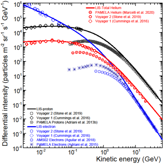
In Figure 6 three examples of the VLISs obtained in this manner are shown, here depicted for protons, electrons and total helium (He-4 plus He-3) at the HP (122 AU) as specified in our modulation model. At high enough KE where solar modulation is assumed insignificant, these VLISs are required to match the observations at Earth. Evidently, as the KE decreases, the deviation of these observations at Earth from the corresponding VLIS increases as solar modulation becomes progressively larger.
4. Positron Modulation
Before the precise, simultaneous and long-term measurements of anti-matter at Earth, charge-sign dependent solar modulation was mostly studied using electrons (negatrons as the sum of electrons and positrons), protons and helium of the same rigidity (e.g., [15]). The first robust observational evidence of charge-sign dependent solar modulation was reported in [138] and modelled in [139] using a drift model which, today, is known as a first generation drift model. These type of drift models predicted that during A > 0 polarity cycles the intensity ratio of negative to positively charged particles as a function of time should exhibit a ∧ shape profile while during A < 0 cycles it should exhibit a ∨ shape around minimum modulation periods, but when only the waviness of the HCS was changed with time [140]; for updates and new insights, see Figure 2 and Figure 3 in [141]. It was found that when other modulation parameters were also changed with time in later generation drift models these distinctive shapes fade and are been smoothed out (e.g., [106]).
Comprehensive modeling was done for electron and positron modulation in the global heliosphere [101,102] relying on the computations of galactic spectra [142,143,144] as alternative to the GALPROP calculations [121]. These modulation models were more advanced and also included the effects of the solar wind TS and the role of the inner heliosheath which was considered state-of-the-art at that time but not much attention was given to comparisons between these modulation predictions and observations at the Earth. This has changed since the first positron spectra from PAMELA [2,113,145] became available. Follow-up simulations done for positrons in [135] were based on new VLISs with the focussed on detailed aspects of the solar modulation of positrons during the extraordinary quiet solar modulation period from 2006–2009. For the first time, a meaningful modulation factor in the heliosphere was computed for positrons, from 50 GeV down to 1 MeV, as well as the electron to positron ratios as a function of time and rigidity for the mentioned period. In the next section, the focus is on contemporary modeling of these GCR positrons.
4.1. The VLIS and Modulated Spectra
A comprehensive numerical study of the modulation of galactic electrons and positrons was reported in [60]. First, they established the VLISs for electrons using the process described above [46] by adjusting the appropriate physics in the web version of the GALPROP code [146] (and references there-in) to reproduce both the observed Voyager 1 and 2 electron intensity levels from beyond the HP and the high KE observations from PAMELA where solar modulation is considered negligible. Since positron data is not available beyond the HP, the spectral shape of the positron VLIS at low KE is based on what GALPROP produced but empirically modified as explained in [45,67] to improve the reproduction of observed spectra at Earth. As mentioned, the only known differences in the heliospheric modulation of electrons and positrons are the particle drifts that they experience and their respective VLISs.
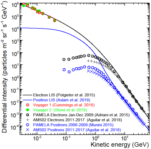
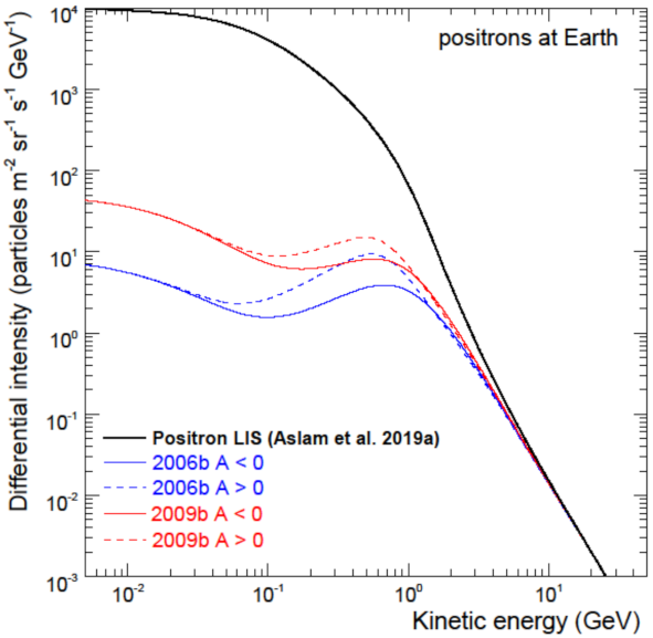
The computed VLIS for electrons and positrons are shown in Figure 7 together with observations for galactic electrons from PAMELA from January to December 2009 [82], from AMS-02 from May 2011 to May 2017 [5] and from Voyager 1 [6,19] and Voyager 2 [7], with positron observations from PAMELA [113] and AMS-02 [5]. As for Figure 6, solar modulation is assumed insignificant at high enough KE where these VLISs are required to match the Earth observations. Again, the deviation of these observations at the Earth from the corresponding VLISs increases as solar modulation becomes progressively larger with decreasing KE.
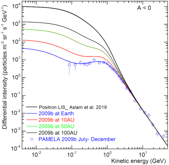
In Figure 8, the modulation of positrons during extraordinary quite modulation conditions is shown as computed spectra at Earth compared to PAMELA data [113] for the period July to December 2009 (A > 0 cycle), and corresponding computed spectra throughout the heliosphere at 10 AU, 50 AU and 100 AU in the equatorial plane with respect to the VLIS at 122 AU. Examples of how large this modulation may be for an A > 0 cycle were given in [67], which can be tested once AMS-02 positron spectra are published for the present solar minimum period. Neutron monitors at ground level have already reached maximum counts in mid-2020 (see, e.g., [147]).
4.2. Drift Effects
Figure 9 illustrates the predicted drift effects relevant to positrons displayed as computed spectra at Earth for modulation conditions applicable to the second halves of 2006 and 2009 (indicated as 2006b and 2009b) for the A < 0 cycle compared to the A > 0 cycle assuming the same modulation conditions. These spectra are shown with respect to the assumed VLIS at 122 AU. Evidently, focussing on the qualitative features, drift effects gradually subside with decreasing KE to vanish completely at low enough KE. For increasing and higher KE these effects gradually subside to become relatively small above a few GeV. This happens differently at higher KE than at the lower KE. Important is that the intensity for A > 0 cycles is predicted consistently higher than for A < 0 cycles, under the same modulation conditions, but not at all rigidities; note that the subtle phenomenon of the cross-over of these A > 0 and A < 0 spectra between 1–2 GeV is also present for these GCRs so that it is not obvious where these drift effects completely disappear with increasing KE. Modelling details related to this figure were reported in [45].
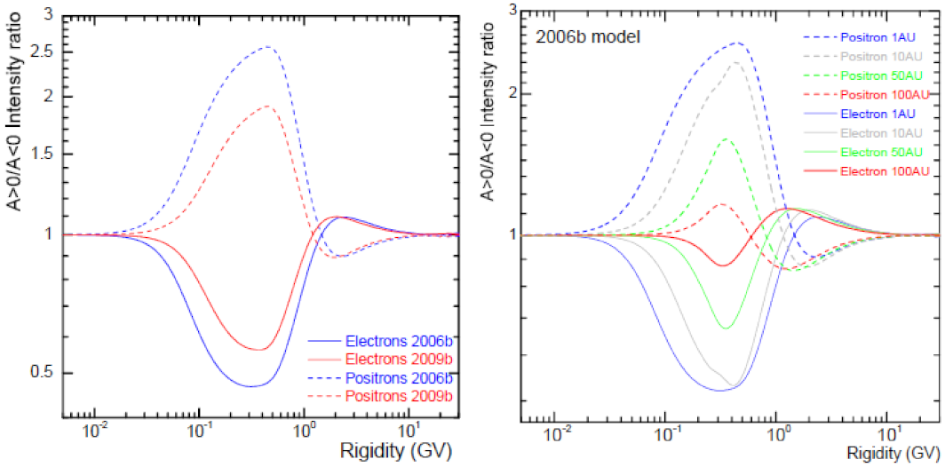
The quantitative features are displayed in Figure 10 by plotting the ratio of intensities for A < 0 to A < 0, first for the periods 2006b and 2009b for both electrons and positrons. In the left panel the ratios are shown at Earth related to Figure 9. The largest drift effects are occurring between 200 MV and 600 MV, progressively phasing out with decreasing rigidity to fade away below ~100 MV. Drift effects also subside with increasing rigidity (KE), but more strongly than at low rigidity, producing in the process the spectral cross-over phenomenon. As mentioned above, the inspection of the difference between A > 0 and A < 0 spectra above 1–2 GV in Figure 9 shows this cross-over, clearly evident in the ratios, so that A < 0 becomes higher than A > 0, in contrast to what happens at lower rigidity (KE). It appears that drift effects dissipate above ~10 GV but how small it gets before completely subsiding still needs to be investigated thoroughly (related to which rigidity solar modulation really commences at). In the right panel of Figure 10 the predicted ratios are shown at 10 AU, 50 AU and 100 AU in the equatorial plane, in addition to those at 1 AU. Evidently, drift effects decrease with increasing radial distance, from a maximum ratio of ~2.5 at 1 AU to ~1.2 at 100 AU; see also [35,148] who simulated drift effects for GCRs throughout the heliosphere. These results are consistent to what [84] reported for drift effects on electrons; see also predictions made for the two drift cycles for electrons and protons in [111].
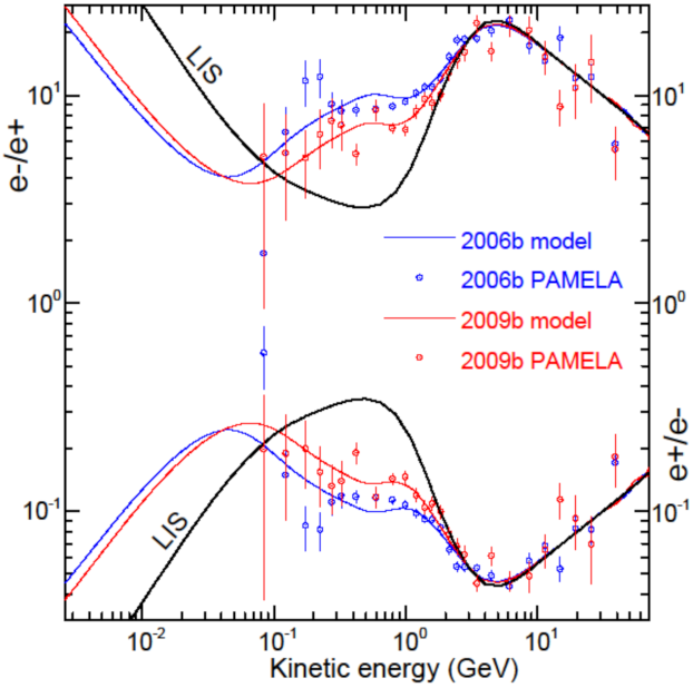
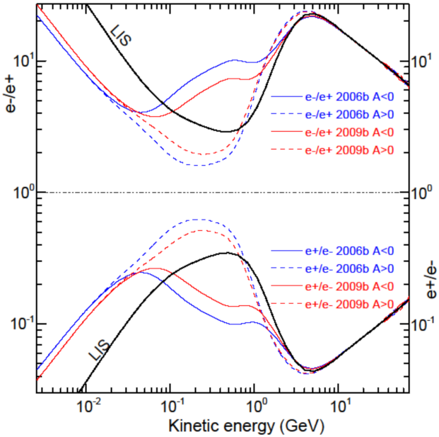
The charge-sign dependence displayed in Figure 10 is further highlighted in the next two figures by plotting the ratio of electron to positron intensities (e−/e+) as a function of KE, as well as for (e+/e−) in the bottom parts for illustrative purposes because it has been reported as such many times. These computed ratios are shown in Figure 11 at Earth with respect to the ratio of the two respective VLIS. The simulations are done for 2006b and 2009b modulation conditions so that a comparison can be made to the PAMELA observations [2,113] of electrons and positrons for these well-defined solar minimum periods. In Figure 12, these ratios are repeated for the A < 0 cycle as shown in Figure 11 but now also including the predicted ratios for an A > 0 drift cycle (the present solar epoch) assuming modulation conditions to be the same as in 2006b and 2009b. This serves to highlight the difference in these ratios between the two drift cycles.
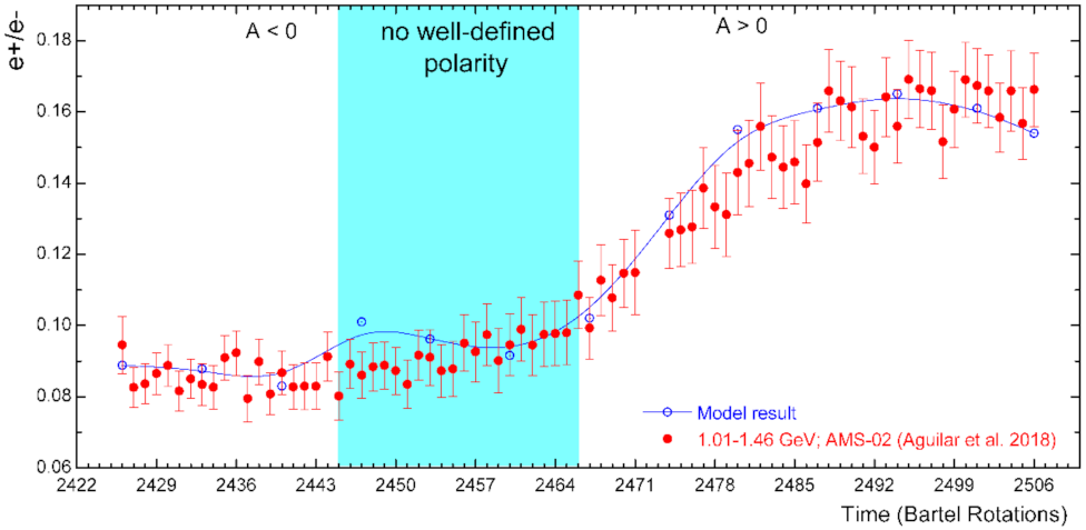
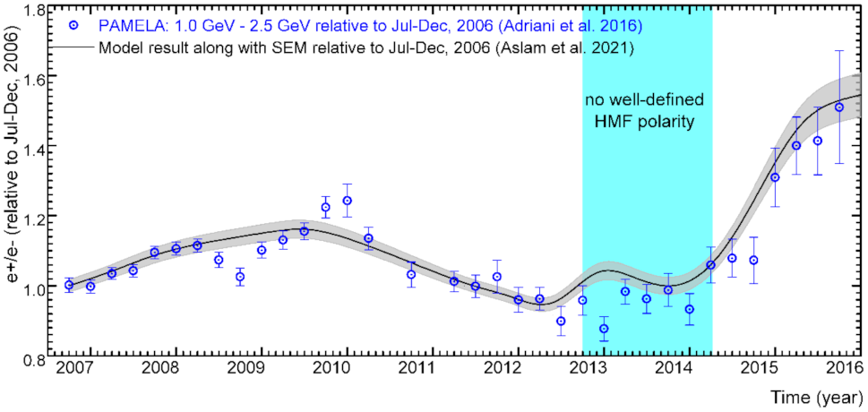
An illustration of how charge-sign dependent modulation changes with time (solar activity), the observed and simulated ratios (e+/e−) are shown in Figure 13 for 1.01–1.46 GeV and for Bartels rotation numbers 2426 to 2506 (mid-2011 to mid-2017). The simulated ratios are based on reproducing the AMS-02 electron and positron spectra for these periods. Evidently, the simulations agree well with the observations displaying how the ratio changes from a low value before the reversal period to a significantly higher value afterwards. Figure 14 shows simulated ratios based on reproducing the observed PAMELA ratio [2] for 1.01–2.5 GeV over a longer period from 2006 to 2016. Modelling details related to this figure were reported in [60].
5. Anti-Proton Modulation
The first prediction of drift effects pertinent to anti-proton modulation was made in [149]. This early, first generation drift model, with the HP assumed at only 50 AU, predicted a change of a factor of ~8 in the anti-proton to proton ratio at 300 MeV between an A > 0 minimum and an A < 0 solar minima but about half of that for periods of increased solar activity. The LIS for protons and anti-protons were typical of what had been used then. The only time-dependent change in this modulation model was the tilt angle so what was predicted for solar maximum conditions was significantly over estimated. Comprehensive modeling was later done for anti-proton modulation in [101,102,150] relying on computations of galactic spectra with the GALPROP code [122]. Apart from drifts, their model also included the effects of the TS and the role of the outer heliosheath. These models predicted lesser drift effects than first generation models but they also consistently applied an overall reduction factor to the drift coefficient. The modulated anti-proton spectra at Earth reported in [102] differed by a factor of 1.5 below 100 MeV between the two drift cycles and also illustrated how the anti-proton to proton ratio changed from solar minimum to maximum.
Later, a 3D modulation model was used in [93] based on solving SDEs to study the modulation of protons and anti-protons and found a maximum drift effect of a factor of ~10 below ~100 MeV which gradually subsides with increasing KE to become negligible above 10 GeV. These predicted effects are large so that no attention was then given to smaller modulation effects above a few GeV as is done nowadays with the availability of precise GCR spectra. Recently, aspects of the modeling of anti-protons were reported in [28,119,151]; the latter raising additional questions about what the VLIS for anti-protons may be. In what follows the modelling study given here is described based on the approach outlined in this paper on how to obtain what can be considered a realistic anti-proton VLIS for solar modulation studies.
To recap concisely, the approach mentioned above is focus on gauging the numerical model and validating the modulation parameters on reproducing the observed protons and helium spectra at the HP at low KE and at Earth at much higher KE; see also [48,49,50,51]. The model is then applied to anti-protons with the assumption that there is no fundamental reason for anti-protons to be differently modulated than protons apart from the drift field directions that changes every 11 years. It is thus implied that anti-protons have the exact same MFPs as well as the drift scale than protons but oppositely directed drift velocity fields.
5.1. The Anti-Proton VLIS and Modulated Spectra
The numerical modeling described here is focussed on the PAMELA anti-proton spectra averaged from 2006 to 2009 to obtain improved statistics [145,152,153] which as such has less uncertainty than observations reported before this mission. The availability of very precise proton spectra for the same period and from the same detector makes the gauging process of the modeling much easier. The physics in the GALPROP code is adjusted to determine two possible anti-proton LISs which is then used in the modulation code at 122 AU to compute the corresponding modulated spectra at Earth based on the equivalent study of proton modulation. The procedure, followed here, including the adjustment of relevant physics in GALPROP, is described in [46,57]. It is worth mentioning that doing this for positrons and anti-protons is more complicated because they are secondary GCRs thus influenced by how they are created in galactic space through nuclear cross-sections. The two LISs computed with GALPROP are the plain diffusion (PD) and the reacceleration (REAC) approach, the latter being our preferred model for computing the LIS for protons. These two LISs are shown in Figure 15, the PD-model considered as the upper limit (black dotted line) and the REAC-model as the lower limit (black dashed line). The corresponding modulated spectra at Earth are computed based on the modulation parameters that worked optimally for protons for the solar minimum period 2009. These modulated spectra are compared to the mentioned PAMELA data. Inspection of these results shows that the REAC-model produces a LIS, specified in our modulation model as the HP (122 AU), that goes through the observational data at the Earth and thus fails to be considered as a realistic VLIS in our opinion. The PD-model gives a modulated spectrum significantly above the observations, which we anticipated because the same result was found for protons. This dilemma causes us to calculate an averaged VLIS (black solid line), using the two mentioned GALPROP spectra, and of which the corresponding modulated spectrum (red solid line) reproduces the observations reasonably well. We also repeated the modulation part using modulation conditions as found for protons for 2006 but found less agreement with these anti-proton observations; this modulated spectrum is found a factor 0.8 lower at its peak value. We therefore decided to settle on this averaged LIS (called LIS 3, Adjust, in this figure) as the optimal VLIS for further anti-proton modulation studies below 1 GeV. Adding earlier observations for anti-protons from balloon flights to this picture did not provide additional modulation insight and are not shown; see reviews of these earlier observations in, e.g., [145,154,155].
The modulation of anti-protons between the HP and the Earth, as illustrated in Figure 15, requires some additional remarks because it is rather peculiar in the sense that:
- (1)
- The shape of the VLIS is quite different from GCR nuclei, having between 500 MeV and 1 GeV a spectral slope close to the slope evident in the modulated spectra below 500 MeV at Earth. This slope at Earth is caused by adiabatic energy losses inside the heliosphere and is a characteristic of modulated spectra for protons, anti-protons and all GCR nuclei (see also [48]). The shape of the VLIS of these particles below 200 MeV is therefore not reflected at Earth because of these energy losses inside the heliosphere; for illustrations of this modulation effect, see, e.g., [25,156].
- (2)
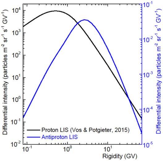
- The total amount of modulation for anti-protons is far less than for protons of the same rigidity because of the very different shape of their VLISs, which for interest sake is compared to the VLIS for protons in Figure 16. As alluded to above, note where the peak in the anti-proton VLIS occurs compared to that for protons and how completely different the spectral slopes are at both low and high rigidities. The VLIS for protons is computed with GALPROP and normalized to PAMELA data at 100 GeV but the anti-proton spectrum is adjusted as described above.
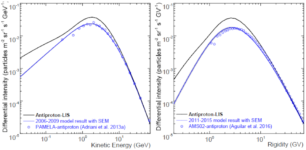
The computed, modulated anti-proton spectra at the Earth are shown in Figure 17 with respect to the assumed VLIS at 122 AU for anti-protons in both panels. Here, they are compared to AMS-02 observations averaged over the period 19 May 2011 to 26 May 2015 [4] in the left panel and to PAMELA observations on the right-side as in Figure 15, repeated here in a less cluttered panel. Although the modulated spectrum for 2006–2009 is in good agreement with the PAMELA data, the corresponding modulated spectrum for 2011–2015 is not agreeing at all rigidities with the AMS-02 observations. It is still quite reasonable in our view, given that the period after 2009 had experienced increased solar activity so that averaging over such a relatively long period makes the reproduction of observations more challenging. When applying our model for maximum solar activity conditions such as in early 2014, the peak value of the modulated anti-proton differential intensity in units as shown in Figure 17, drops to ~1.3 × 10⁻² at 2 GeV whereas at a 100 MeV it drops to ~1.2 × 10⁻³ and at 10 MeV to ~1.2 × 10⁻⁴.
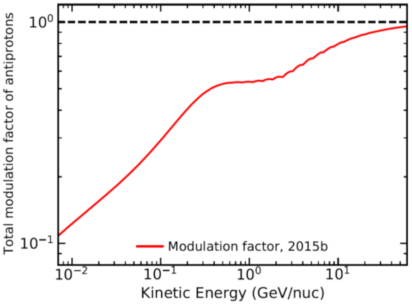
The total modulation factor for anti-protons is shown in Figure 18; this is the factor that the VLIS is reduced between the HP and Earth because of solar modulation as a function of KE and computed for the period 2015b (averaged over the last six months of 2015) when B at the Earth was observed to be at a maximum. This factor thus represents the total modulation over a distance of 121 AU during solar maximum modulation conditions. In this case solar modulation was assumed in the model to commence at 100 GeV. Compared to the simulated modulation factor for protons and electrons [27] and for positrons [45], this factor for anti-protons is much less at low KE and depicts a peculiar form (flatness) from ~300 MeV to around 2 GeV which is absent for protons.
For the time being, we prefer to refrain from adjusting the VLIS for anti-protons simply to produce a better fit to the averaged AMS-02 data as shown in Figure 17; see [157]. The averaging of observational data over long periods is a complicating aspect when precise modeling is an objective. However, this issue remains important so we hope that observations which are analysed on a shorter observational time–scale will become available for the present solar minimum period.
5.2. Charge-Sign Dependence
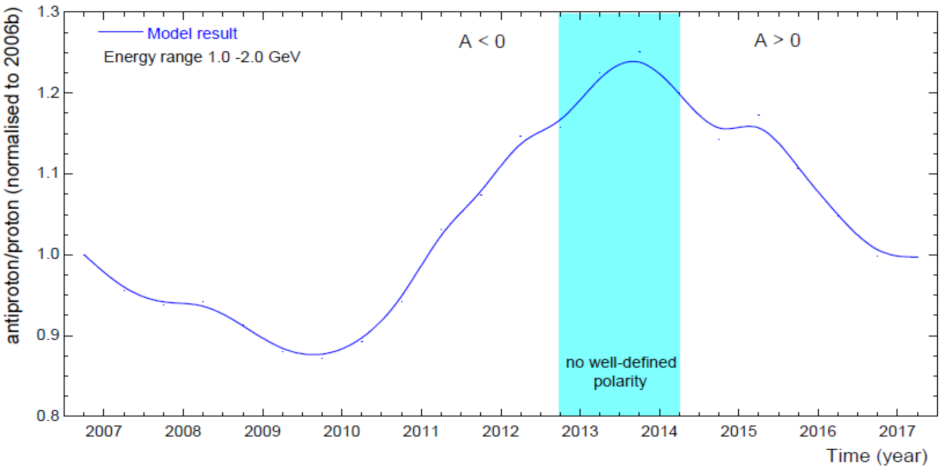
After reproducing the AMS-02 proton and averaged anti-proton spectra, the subsequent anti-proton to proton ratio was calculated (simulated) as a function of time, from 2011–2017, for KE of 1.0–1.5 GeV. This is shown in Figure 19, with the ratio normalized to the value in 2006. It follows that this ratio increases gradually from 2011 to 2017, to reach a maximum in Nov-Dec 2013, and then decreases back to a minimum in Jan 2017. In order to reproduce the AMS-02 ratio, and in addition to varying the DCs (shown in Figure 4), we had to keep the drift scale (or drift coefficient) at a minimum level for the solar maximum period, and then had to increase it gradually to a maximum value as solar activity decreases to a minimum. What is shown here relates to what was shown in Figure 5 for the drift scale, at its maximum value during the 2006–2009 minimum epoch to decrease gradually up to its smallest value for the 2012–2014 reversal period, and then increasing gradually back to a maximum value in Dec 2016.
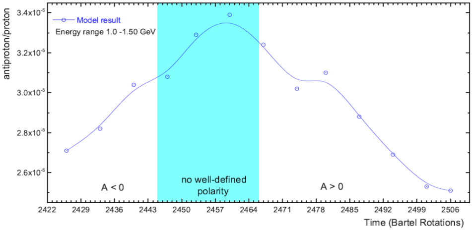
The numerical simulations for the anti-proton to proton variation with time reported in [158] produced large jumps during solar maximum period associated with the change in the HMF polarity because in their modeling approach drift was not changed with solar activity, similar to what was done with first generations drift models before the Ulysses mission [15,16,17,33]; see, e.g., [149]. The simulated anti-proton to proton ratio, not normalized and for a shorter time scale, is repeated in Figure 20 for the KE range 1.0–1.5 GeV as a function of time given by Bartels rotation numbers from 2426 to 2506 (May 2011 to May 2017) as reported by AMS-02.
Let us emphasize that in order to obtain these ratios over time it is necessary to adjust the DCs and very specifically the drift coefficient systematically over time, with the latter becoming very small during the HMF polarity reversal period; see also Figure 4 and Figure 5 above. This modeling study highlights the modulation differences between anti-protons and protons especially for the reversal period. In the next section, the focus will be on the difference between positron and anti-proton modulation.
6. Differences between Positron and Anti-Proton Modulation
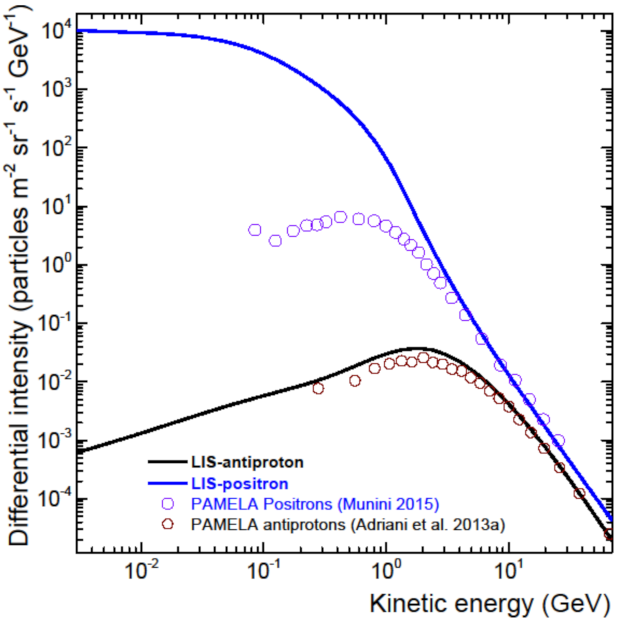
A display of the main differences between positron and anti-proton modulation needs to start off with showing the enormous difference between the positron and anti-proton VLISs as used for this study. This is shown in Figure 21 in comparison with observations from PAMELA [113,152,153], illustrative of the observed positron and anti-proton spectra at the Earth based on the total modulation from 1 AU up to the HP at 122 AU during solar minimum conditions. Evidently, these two VLISs differ significantly the lower the KE, with the positron intensity exceeding the anti-proton intensity by a factor of up to 107 below 10−2 GeV. In contrast, the electron intensity exceeds the proton intensity by a factor of maximum 10 at this KE [111,135].
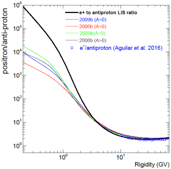
6.1. Positron to Anti-Proton Ratio as a Function of Rigidity
Figure 22 displays the ratio of the VLISs of positrons and anti-protons (solid black line) together with the corresponding simulated positron to anti-proton modulated ratio at the Earth for modulation conditions as in 2006b (red lines) and 2009b (blue lines), for both drift cycles A < 0 and A > 0. The latter serves as predictions for the present solar minimum epoch. The observational ratio above 1 GV is from [4], matching the simulations reasonably well. The difference between the A < 0 and A > 0 cycles is indicative of the extent of drift effects for these GCRs, evidently becoming quite large below 1 GV. These differences relate to what was shown in Figure 2, according to which the positron modulation is dominated by diffusion at lower rigidity (with relatively large and steady MFPs) in contrast to anti-proton modulation which is dominated by adiabatic energy losses at low rigidities as the MFPs get systematically smaller with decreasing rigidity. The causes of these modulation effects are similar to the differences between electron and proton modulation [111] except for the charge-sign dependence which is not at play between positrons and anti-protons.
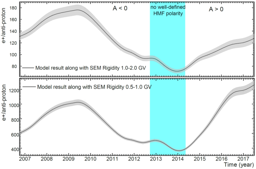
6.2. Positron to Anti-Proton Ratio as a Function Time
The time dependence of the simulated positron to anti-proton ratio is shown in Figure 23 at two rigidity intervals: 1.0–2.0 GV (top panel) and 0.5–1.0 GV (bottom panel). The standard error of mean (SEM; standard deviation/√n) is shown here for the modeling results (solid line with shaded grey band). Evidently, the largest values are obtained in 2009 with the smallest values during solar maximum activity, at the beginning of the reversal period. The variation with time is mainly because of the relatively larger modulation the positrons experience in contrast to the awkward behaviour of the anti-protons as described in relation to Figure 17. The large difference in the ratio values between these two adjacent rigidity intervals is conspicuous and illustrative of how the vast the difference become between the modulated spectra for these two types of anti-particles, also evident in Figure 21 and Figure 22.
7. On the Modulation of Other Types of Anti-Matter
A way to test dark matter annihilation may be found in observations at the Earth of low-energy anti-nuclei in GCRs, such as anti-protons (see [154] describing BESS as one of the early ground-breaking anti-matter experiments), also anti-deuteron and anti-helium (e.g., [159]), which makes proper, realistic and precise modulation modeling eminent. This requires the study of all four major modulation processes including particle drifts that creates a 22-year modulation cycle, which is not described by the Force-Field approach to solar modulation. Applying a drift model to anti-deuteron (e.g., [160,161]) is in reach once the modulation of deuteron can be done properly with the modeling approach used here and when relevant precise spectral observations are published (e.g., [162,163]). Estimates exist for the LIS for deuteron and anti-deuteron (e.g., [164], and references there-in) and some effort has already been made for deuteron modulation modeling as shown in [57] based on deuteron observations at the HP from Voyager 1 [21] and from PAMELA [136,165] but only over a limited energy range. A next step in precise modeling should include the study of the solar modulation of anti-helium (e.g., [166,167]). However, this needs additional and dedicated investigation beyond the scope of the present study.
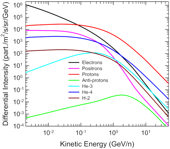
8. A Composition of VLISs
Here, a composition of computed VLISs is provided following the procedure described above for the purpose of pursuing precise global modelling of solar modulation for GCRs, similar to [57]. This is shown in Figure 24 which displays the VLISs for protons, deuteron H-2 (2H1) He-3 (3He2), He-4 (4He2), electrons, and particularly for positrons and anti-protons. It is interesting to note that the VLIS for electrons with KE < ~80 MeV has the largest flux of all GCRs so the question arises what the electron LIS may be down to 1 MeV and at even lower KE? Studying electron modulation to this very low energy at the Earth is difficult because adiabatic energy losses becomes large for electrons only with KE below their rest energy, apart from the dominating presence of Jovian electrons in the inner heliosphere below ~50 MeV [83,84,168,169]. The large flux of positrons below ~300 MeV, even larger than the flux for He-4 is worth noting whereas the H-2 flux is significantly larger than for He-3 below ~200 MeV/n. Not surprising is the low position of the anti-proton VLIS in this hierarchy of astrophysical charged particles.
The VLIS for deuteron as displayed in Figure 24 is not considered as the final word. However, we are confident that the VLISs for protons, anti-protons, electrons, positrons and total He (sum of both isotopes) are already close to what may be considered as optimal for solar modulation studies. Small adjustments to these VLISs at high rigidities, above a few GeV/n, may be required as the study of very small modulation effects at these high rigidities get better, again owing to these precise measurements being made at Earth and the accompanying precise modeling of the total modulation of GCRs in the heliosphere. Qualitatively, minor adjustments will not affect the obtained results on the computed charge-sign dependent ratios as a function of rigidity as shown in Figure 10 to Figure 16 for electrons and positrons and for protons and anti-protons in Figure 19 and Figure 20.
Since we focus on the refinements of VLISs to be used in heliospheric modulation models, no discussion on how astrophysical aspects can change LISs and how that relates to the VLIS specified at the HP is done here. Examples of such details can be found, e.g., in [159,160,164,170,171,172]. If such studies would produce VLISs which were significantly different in terms of their spectral shapes (rigidity dependence) from what is presented here, they should be evaluated with comprehensive modulation models to determine their impact on the results obtained.
9. Summary and Conclusions
Determining the global and total modulation of GCRs in the heliosphere more meticulously than before has become possible because aspects such as the position of the TS and especially the HP are reasonably settled. Consensus on the actual shape of the heliosphere has not yet been reached (e.g., [12]) but so far there exists no conclusive evidence that the shape of the heliosphere [34,148] plays a real dominant role in the total modulation of GCRs observed at Earth.
Sophisticated solar modulation modelling of protons, electrons and total Helium has made it possible to refine the VLISs for all GCR nuclei, with the emphasis in this study on positrons and anti-protons. This approach, together with precise observations at Earth, contribute in restraining the uncertainties in the VLIS even for GCRs not observed by the Voyager spacecraft beyond the HP. Evidently, global modulation studies with comprehensive numerical models contribute meaningfully to the testing and refinement of the VLISs for GCRs.
The modeling presented here includes the effects of the solar magnetic field changing it’s ‘polarity’ to create a 22-year modulation cycle and illustrates differences in how positrons and anti-protons are modulated over time and specifically how much particle drifts they experience which is significant at kinetic energies lower than a few GeV. Because the VLIS for anti-protons has a very peculiar spectral shape in contrast to the one for protons, the total modulation of anti-protons is awkwardly different compared to that for protons and other GCR nuclei.
The total modulation factor for anti-protons as a function of KE at Earth is computed with respect to the VLIS specified at the HP (122 AU); see Figure 18. The detailed anti-proton to proton ratio as a function of solar activity is computed for an 11-year period and serves as a prediction of what happens over periods of extreme solar activity and a change in the HMF polarity (Figure 19 and Figure 20). This prediction deviates from other predictions on how this ratio changes during maximum solar activity; see, e.g., [149,158,173]. We found that this ratio decreases generally with decreasing solar activity and increases with increasing solar activity to reach a peak value during maximum solar activity, making a gradual change towards a peak value during this period. This ratio at 1–2 GeV may change as much as a factor of 1.5 over a solar cycle and the differential intensity for anti-protons may decrease by a factor of 2 at 100 MeV from solar minimum to solar maximum. Acquiring these charge-sign dependent ratios over time at the Earth it is necessary to adjust the heliospheric DCs and very specifically the drift coefficient systematically with solar activity, with the latter becoming quite small during the HMF polarity reversal period; see Figure 2, Figure 3, Figure 4 and Figure 5.
The ratio of the VLISs of positrons to anti-protons are determined together with the corresponding simulated positron to anti-proton ratio at the Earth, based on modulation conditions that existed in 2006 and 2009, done for both drift cycles, A < 0 and A > 0. The latter serves as predictions for the present solar minimum epoch.
A composition of computed VLISs is given in Figure 24 for the purpose of pursuing precise global modelling of solar modulation for these GCRs. It follows that the VLIS for electrons with KE < ~80 MeV has the largest flux of all GCRs with the anti-proton flux by far the lowest.
Author Contributions
Conceptualization, M.S.P.; methodology, all authors; software, O.P.M.A., D.B., D.N.; validation, all authors; analysis, all authors; writing—original draft preparation, M.S.P.; writing—review and editing, all authors; visualization, all authors; supervision, M.S.P.; project administration, D.N., M.S.P.; funding acquisition, D.N. All authors have read and agreed to the published version of the manuscript.
Funding
M.D.N. thanks the South African (SA) National Research Foundation (NRF) for his partial financial support under Joint Science and Technology Research Collaboration between SA and Russia (Grant No: 118915) and BAAP (Grant No: 120642). He acknowledges that the opinions, findings, conclusions or recommendations expressed in publication generated by SA NRF supported research is that of the authors alone, and that the SA NRF accepts no liability whatsoever in this regard. D.B. and O.P.M.A. acknowledge the financial support they had received from the NWU’s post-doctoral programme.
Conflicts of Interest
The authors declare no conflict of interest.
References
- Adriani, O.; Barbarino, G.C.; Bazilevskaya, G.A.; Bellotti, R.; Boezio, M.; Bogomolov, E.A.; Bonechi, L.; Bongi, M.; Bonvicini, V.; Borisov, S.; et al. PAMELA results on the cosmic-ray antiproton flux from 60 MeV to 180 GeV in kinetic energy. Phys. Rev. Lett. 2010, 105, 121101. [Google Scholar] [CrossRef] [PubMed]
- Adriani, O.; Barbarino, G.C.; Bazilevskaya, G.A.; Bellotti, R.; Boezio, M.; Bogomolov, A.E.; Bongi, M.; Bonvicini, V.; Bottai, S.; Bruno, A.; et al. Time dependence of the electron and positron components of the cosmic radiation measured by the PAMELA experiment between July 2006 and December 2015. Phys. Rev. Lett. 2016, 116, 241105. [Google Scholar] [CrossRef] [PubMed] [Green Version]
- Adriani, O.; Barbarino, G.C.; Bazilevskaya, G.A.; Bellotti, R.; Boezio, M.; Bogomolov, A.E.; Bongi, M.; Bonvicini, V.; Bottai, S.; Bruno, A.; et al. Ten years of PAMELA in space. La Riv. Del Nuovo Cim. 2017, 40, 473–522. [Google Scholar] [CrossRef]
- Aguilar, M.; Ali Cavasonza, L.; Alpat, B.; Ambrosi, G.; Arruda, L.; Attig, N.; Aupetit, S.; Azzarello, P.; Bachlechner, A.; Barao, F.; et al. Antiproton flux, antiproton-to-proton flux ratio, and properties of elementary particle fluxes in primary cosmic rays measured with the Alpha Magnetic Spectrometer on the International Space Station. Phys. Rev. Lett. 2016, 117, 091103. [Google Scholar] [CrossRef] [PubMed]
- Aguilar, M.; Ali Cavasonza, L.; Ambrosi, G.; Arruda, L.; Attig, N.; Aupetit, S.; Azzarello, P.; Bachlechner, A.; Barao, F.; Barrau, A.; et al. Observation of complex time structures in the Cosmic-ray electron and positron fluxes with the Alpha Magnetic Spectrometer on the International Space Station. Phys. Rev. Lett. 2018, 121, 051102. [Google Scholar] [CrossRef] [Green Version]
- Stone, E.C.; Cummings, A.C.; McDonald, F.B.; Heikkila, B.C.; Lal, N.; Webber, W.R. Voyager 1 observes low-energy galactic cosmic rays in a region depleted of heliospheric ions. Science 2013, 341, 150–153. [Google Scholar] [CrossRef] [PubMed]
- Stone, E.C.; Cummings, A.C.; Heikkila, B.C.; Lal, N. Cosmic ray measurements from Voyager 2 as it crossed into interstellar space. Nature Astron. 2019, 3, 1013–1018. [Google Scholar] [CrossRef]
- Kóta, J.; Jokipii, J.R. Are cosmic rays modulated beyond the heliopause? Astrophys. J. 2014, 782, 1–6. [Google Scholar] [CrossRef] [Green Version]
- Luo, X.; Potgieter, M.S.; Zhang, M.; Pogorelov, N.; Feng, X.; Strauss, R.D. A numerical simulation of cosmic ray modulation near the heliopause: II. Some physical insights. Astrophys. J. 2016, 826, 182. [Google Scholar] [CrossRef] [Green Version]
- Zhang, M.; Pogorelov, N.V. Modulation of galactic cosmic rays by plasma disturbances propagating through the Local Interstellar Medium in the outer heliosheath. Astrophys. J. 2020, 895, 1. [Google Scholar] [CrossRef]
- Scherer, K.; Fichtner, H. The return of the bow shock. Astrophys. J. 2014, 782, 25. [Google Scholar] [CrossRef] [Green Version]
- Pogorelov, N.; Fichtner, H.; Czechowski, A.; Lazarian, A.; Lembege, B.; le Roux, J.A.; Potgieter, M.S.; Scherer, K.; Stone, E.C.; Strauss, R.D.; et al. Heliosheath processes and the structure of the heliopause modeling energetic particles, cosmic rays, and magnetic fields. Space Sci. Rev. 2017, 212, 193–248. [Google Scholar] [CrossRef] [Green Version]
- Schlickeiser, R.; Oppotsch, J.; Zhang, M.; Pogorelov, N.V. On the anisotropy of galactic cosmic rays. Astrophys. J. 2019, 879, 29. [Google Scholar] [CrossRef]
- Zhang, M.; Pogorelov, N.V.; Zhang, Y.; Hu, H.B.; Schlickeiser, R. The original anisotropy of TeV Cosmic Rays in the Local Interstellar Medium. Astrophys. J. 2020, 889, 97. [Google Scholar] [CrossRef]
- Heber, B.; Wibberenz, G.; Potgieter, M.S.; Burger, R.A.; Ferreira, S.; Müller-Mellon, R.; Kunow, H.; Ferrando, P.; Raviart, A.; Paizis, C.; et al. Ulysses cosmic ray and solar particle investigation/Kiel Electron Telescope observations: Charge sign dependence and spatial gradients during the 1990–2000 A > 0 solar magnetic cycle. J. Geophys. Res. 2002, 107, 1274. [Google Scholar] [CrossRef]
- Heber, B.; Kopp, A.; Gieseler, J.; Müller-Mellin, R.; Fichtner, H.; Scherer, K.; Potgieter, M.S.; Ferreira, S.E.S. Modulation of galactic cosmic ray protons and electrons during an unusual solar minimum. Astrophys. J. 2009, 699, 1956–1963. [Google Scholar] [CrossRef]
- Heber, B.; Potgieter, M.S. Cosmic rays at high heliolatitudes. Space Sci. Rev. 2006, 127, 117–194. [Google Scholar] [CrossRef]
- Heber, B.; Potgieter, M.S. Galactic and anomalous cosmic rays through the solar cycle: New insights from Ulysses. In The Heliosphere through the Solar Activity Cycle; Balogh, A., Lanzerotti, L.J., Suess, S.J., Eds.; Springer: Berlin/Heidelberg, Germany, 2008; pp. 195–249. [Google Scholar] [CrossRef]
- Cummings, A.C.; Stone, E.C.; Heikkila, B.C.; Lal, N.; Webber, W.R. Galactic cosmic rays in the local interstellar medium: Voyager 1 observations and model results. Astrophys. J. 2016, 831, 18. [Google Scholar] [CrossRef] [PubMed] [Green Version]
- Webber, W.R.; Villa, T.L. A comparison of the galactic cosmic ray electron and proton intensities from 1 MeV/nuc to 1 TeV/nuc using Voyager and higher energy magnetic spectrometer measurements; Are there differences in the source spectra of these particles? arXiv 2018, arXiv:1806.02808. [Google Scholar]
- Webber, W.R.; Lal, N.; Heikkila, B. The spectra of 2H and 3He secondary cosmic ray isotopes from ~20-85 MeV/nuc as measured using the B-end HET Telescope on Voyager beyond the heliopause and a fit to these Interstellar Spectra using a Leaky Box Propagation Model. arXiv 2018, arXiv:1802.08273. [Google Scholar]
- Strauss, R.D.; Potgieter, M.S. Where does the heliospheric modulation of galactic cosmic rays start? Adv. Space Res. 2014, 53, 1015–1023. [Google Scholar] [CrossRef]
- Gleeson, L.J.; Urch, I.A. A study of the force-field equation for the propagation of galactic cosmic rays. Astrophys. Space Sci. 1973, 25, 387–404. [Google Scholar] [CrossRef]
- Cholis, I.; Hooper, D.; Linden, T. A predictive analytic model for the solar modulation of cosmic rays. Phys. Rev. D. 2016, 93, 043016. [Google Scholar] [CrossRef] [Green Version]
- Caballero-Lopez, R.A.; Moraal, H. Limitations of the force field equation to describe cosmic ray modulation. J. Geophys. Res. 2004, 109, A01101. [Google Scholar] [CrossRef]
- Moraal, H. Cosmic-ray modulation equations. Space Sci. Rev. 2013, 176, 299–319. [Google Scholar] [CrossRef]
- Potgieter, M.S. The global modulation of cosmic rays during a quiet heliosphere: A modeling perspective. Adv. Space Res. 2017, 60, 848–864. [Google Scholar] [CrossRef]
- Engelbrecht, N.E.; di Felice, V. Uncertainties implicit to the use of the force-field solutions to the Parker transport equation in analyses of observed cosmic ray antiproton intensities. Phys. Rev. D 2020, 102, 103007. [Google Scholar] [CrossRef]
- Parker, E.N. The passage of energetic charged particles through interplanetary space. Planet. Space Sci. 1965, 13, 9–49. [Google Scholar] [CrossRef]
- Smith, C.W.; Bieber, J.W. Solar cycle variation of the interplanetary magnetic field spiral. Astrophys. J. 1991, 370, 435. [Google Scholar] [CrossRef]
- Raath, J.L.; Potgieter, M.S.; Strauss, R.D.; Kopp, A. The effects of magnetic field modifications on the solar modulation of cosmic rays with a SDE-based model. Adv. Space Res. 2016, 57, 1965–1977. [Google Scholar] [CrossRef] [Green Version]
- McComas, D.J.; Elliot, H.A.; Gosling, J.T.; Reisenfield, D.B.; Skoung, R.M.; Goldstein, B.E.; Neugebauer, M.; Balogh, A. Ulysses’ second fast latitude scan: Complexity near solar maximum and the reformation of polar coronal holes. Geophys. Res. Lett. 2002, 29, 1. [Google Scholar] [CrossRef]
- Heber, B. Cosmic rays through the solar Hale Cycle. Insights from Ulysses. Space Sci. Rev. 2013, 176, 265–278. [Google Scholar] [CrossRef]
- Langner, U.W.; Potgieter, M.S. The modulation of galactic protons in an asymmetrical heliosphere. Astrophys. J. 2005, 630, 1114–1124. [Google Scholar] [CrossRef]
- Ngobeni, M.D.; Potgieter, M.S. Modulation of galactic cosmic rays in a north-south asymmetrical heliosphere. Adv. Space Res. 2011, 48, 300–307. [Google Scholar] [CrossRef]
- Richardson, J.D.; Wang, C. Plasma in the heliosheath: 3.5 years of observations. Astrophys. J. 2011, 734, L21. [Google Scholar] [CrossRef]
- Stone, E.C.; Cummings, A.C.; McDonald, F.B.; Heikkila, B.C.; Lal, N.; Webber, W.R. Voyager 1 explores the termination shock region and the heliosheath beyond. Science 2005, 309, 2017. [Google Scholar] [CrossRef] [PubMed]
- Richardson, J.D.; Kasper, J.C.; Wang, C.; Belcher, W.; Lazarus, A.J. Cool heliosheath plasma and deceleration of the upstream solar wind at the termination shock. Nature 2008, 454, 63. [Google Scholar] [CrossRef] [PubMed]
- Vos, E.E.; Potgieter, M.S. Global gradients for cosmic ray protons during the solar minimum of cycle 23/24. Solar Phys. 2016, 291, 2181–2195. [Google Scholar] [CrossRef] [Green Version]
- Langner, U.W.; Potgieter, M.S.; Fichtner, H.; Borrmann, T. Effects of solar wind speed changes in the heliosheath on the modulation of cosmic ray protons. Astrophys. J. 2006, 640, 1119–1134. [Google Scholar] [CrossRef]
- Ngobeni, M.D.; Potgieter, M.S. The heliospheric modulation of cosmic rays: Effects of a latitude dependent solar wind termination shock. Adv. Space Res. 2010, 46, 391–401. [Google Scholar] [CrossRef]
- Potgieter, M.S.; Vos, E.E.; Boezio, M.; De Simone, N.; Di Felice, V.; Formato, V. Modulation of galactic protons in the heliosphere during the unusual solar minimum from 2006 to 2009: A modelling approach. Solar Phys. 2014, 289, 391–406. [Google Scholar] [CrossRef] [Green Version]
- Potgieter, M.S.; Vos, E.E.; Munini, R.; Boezio, M.; Di Felice, V. Modulation of galactic electrons in the heliosphere during the unusual solar minimum of 2006 to 2009: A modelling approach. Astrophys. J. 2015, 810, 141. [Google Scholar] [CrossRef]
- Adriani, O.; Barbarino, G.C.; Bazilevskaya, G.A.; Bellotti, R.; Boezio, M.; Bogomolov, E.A.; Bongi, M.; Bonvicini, V.; Borisov, S.; Bottai, S.; et al. Time dependence of the proton flux measured by PAMELA during the 2006 July-2009 December solar minimum. Astrophys. J. 2013, 765, 91. [Google Scholar] [CrossRef] [Green Version]
- Aslam, O.P.M.; Bisschoff, D.; Potgieter, M.S.; Boezio, M.; Munini, R. Modeling of heliospheric modulation of cosmic-ray positrons in a very quiet heliosphere. Astrophys. J. 2019, 873, 70. [Google Scholar] [CrossRef] [Green Version]
- Bisschoff, D.; Potgieter, M.S.; Aslam, O.P.M. New very local interstellar spectra for electrons, positrons, protons, and light cosmic ray nuclei. Astrophys. J. 2019, 878, 59. [Google Scholar] [CrossRef] [Green Version]
- Corti, C.; Potgieter, M.S.; Bindi, V.; Consolandi, C.; Light, C.; Palermo, M.; Popkow, A. Numerical modeling of galactic cosmic ray proton and helium observed by AMS-02 during the solar maximum of Solar Cycle 24. Astrophys. J. 2019, 871, 253. [Google Scholar] [CrossRef]
- Ngobeni, M.D.; Aslam, O.P.M.; Bisschoff, D.; Potgieter, M.S.; Ndiitwani, D.C.; Boezio, M.; Marcelli, N.; Munini, R.; Mikhailov, V.V.; Koldobskiy, S.A. The 3D numerical modeling of the solar modulation of galactic protons and helium nuclei related to observations by PAMELA between 2006 and 2009. Astrophys. Space Sci. 2020, 365, 182. [Google Scholar] [CrossRef]
- Ngobeni, M.D.; Aslam, O.P.M.; Bisschoff, D.; Ndiitwani, D.C.; Potgieter, M.S.; Boezio, M.; Marcelli, N.; Munini, R.; Mikhailov, V.V.; Koldobskiy, S.A. Combined heliospheric modulation of galactic protons and Helium nuclei from solar minimum to maximum activity related to observations by PAMELA and AMS-02. PoS 2021, ICRC2021, 1337. [Google Scholar] [CrossRef]
- Ngobeni, M.D.; Potgieter, M.S.; Aslam, O.P.M.; Bisschoff, D.; Ramokgaba, I.I.; Ndiitwani, D.C. Numerical modeling of the solar modulation of helium isotopes in theiInner heliosphere. PoS 2021, ICRC2021, 1338. [Google Scholar] [CrossRef]
- Ngobeni, M.D.; Potgieter, M.S.; Aslam, O.P.M.; Bisschoff, D.; Ramokgaba, I.I.; Ndiitwani, D.C. Simulations of the solar modulation of helium isotopes constrained by observations. Adv. Space Res. 2021. accepted. [Google Scholar]
- Kóta, J. Theory and modeling of galactic cosmic rays: Trends and prospects. Space Sci. Rev. 2013, 176, 391–403. [Google Scholar] [CrossRef]
- Potgieter, M.S. The modulation of galactic cosmic rays in the heliosphere: Theory and models. Space Sci. Rev. 1998, 83, 147–158. [Google Scholar] [CrossRef]
- Potgieter, M.S. Solar modulation of cosmic rays. Living Rev. Solar Phys. 2013, 10, 3–66. [Google Scholar] [CrossRef] [Green Version]
- Schlickeiser, R. Cosmic Ray Astrophysics; Springer: Berlin/Heidelberg, Germany, 2002. [Google Scholar] [CrossRef]
- Quenby, J.J. The theory of cosmic ray modulation. Space Sci. Rev. 1984, 37, 201–267. [Google Scholar] [CrossRef]
- Bisschoff, D.; Aslam, O.P.M.; Ngobeni, M.D.; Mikhailov, V.V.; Boezio, M.; Munini, R.; Potgieter, M.S. On the very local interstellar spectra for helium, positrons, anti-protons, deuteron and anti–deuteron. Proceedings of the 3rd International Symposium on Cosmic Rays & Astrophysics (ISCRA-2021), Moscow, Russia, 8–10 June 2021. Phys. Atom. Nucl. 2021, 84, 52–58. [Google Scholar] [CrossRef]
- Zhu, C.-R.; Yuan, Q.; Wie, D.-M. Local interstellar spectra and solar modulation of cosmic ray electrons and positrons. Astropart. Phys. 2020, 124, 102495. [Google Scholar] [CrossRef]
- Potgieter, M.S. The charge-sign dependent effect in the solar modulation of cosmic rays. Adv. Space Res. 2014, 53, 1415–1425. [Google Scholar] [CrossRef]
- Aslam, O.P.M.; Bisschoff, D.; Ngobeni, M.D.; Potgieter, M.S.; Munin, I.R.; Boezio, M.; Mikhailov, V.V. Time and charge-sign dependence of the heliospheric modulation of cosmic rays. Astrophys. J. 2021, 909, 215. [Google Scholar] [CrossRef]
- Kopp, A.; Raath, J.-L.; Fichtner, H.; Potgieter, M.S.; Ferreira, S.E.S.; Heber, B. Cosmic-ray transport in heliospheric magnetic structures. III. Implications of solar magnetograms for the drifts of cosmic rays. Astrophys. J. 2021, 922, 124. [Google Scholar] [CrossRef]
- The Wilcox Solar Observatory. Available online: http://wso.stanford.edu (accessed on 1 July 2021).
- Paths to Magnetic Field, Plasma, Energetic Particle Data Relevant to Heliospheric Studies and Resident at Goddard’s Space Physics Data Facility. Available online: http://omniweb.gsfc.nasa.gov (accessed on 1 July 2021).
- Sun, X.; Hoeksema, J.T.; Liu, Y.; Zhao, J. On polar magnetic field reversal and surface flux transport during solar cycle 24. Astrophys. J. 2015, 798, 114. [Google Scholar] [CrossRef]
- Janardhan, P.; Fujiki, K.; Ingale, M.; Bisoi, S.K.; Rout, D. Solar cycle 24: An unusual polar field reversal. Astron. Astrophys. 2018, 618, A148. [Google Scholar] [CrossRef]
- Aslam, O.P.M.; Bisschoff, D.; Potgieter, M.S. The solar modulation of protons and anti-protons. PoS 2019, ICRC2019, 1054. [Google Scholar] [CrossRef]
- Aslam, O.P.M.; Bisschoff, D.; Potgieter, M.S. The heliospheric modulation of electrons and positrons. PoS 2019, ICRC2019, 1053. [Google Scholar] [CrossRef]
- Bieber, J.W.; Matthaeus, W.H.; Smith, C.W.; Wanner, W.; Kallenrode, M.-B.; Wibberenz, G. Proton and electron mean free paths: The Palmer consensus revisited. Astrophys. J. 1994, 420, 294–306. [Google Scholar] [CrossRef]
- Potgieter, M.S. The heliospheric modulation of galactic electrons: Consequences of new calculations for the mean free path of electrons between 1 MeV and ∼ 10 GeV. J. Geophys. Res. 1996, 101, 24411–24422. [Google Scholar] [CrossRef]
- Teufel, A.; Schlickeiser, R. Analytical calculation of the parallel mean free path of heliospheric cosmic rays II. Dynamical magnetic slab turbulence and random sweeping slab turbulence with finite wave power at small wavenumbers. Astron. Astrophys. 2003, 397, 15. [Google Scholar] [CrossRef] [Green Version]
- Shalchi, A. Nonlinear Cosmic Ray Diffusion Theories; Springer: Berlin/Heidelberg, Germany, 2009. [Google Scholar] [CrossRef] [Green Version]
- Ngobeni, M.D.; Potgieter, M.S. Modelling the effects of scattering parameters on particle-drift in the solar modulation of galactic cosmic rays. Adv. Space Res. 2015, 56, 1525–1537. [Google Scholar] [CrossRef]
- Tautz, R.C.; Shalchi, A. Drift coefficient of charged particles in turbulent magnetic fields. Astrophys. J. 2012, 744, 125. [Google Scholar] [CrossRef]
- Engelbrecht, N.E.; Strauss, R.D.; le Roux, J.A.; Burger, R.A. Toward a greater understanding of the reduction of drift coefficients in the presence of turbulence. Astrophys. J. 2017, 841, 107. [Google Scholar] [CrossRef] [Green Version]
- Manuel, R.; Ferreira, S.E.S.; Potgieter, M.S.; Strauss, R.D.; Engelbrecht, N.E. Time-dependent cosmic ray modulation. Adv. Space Res. 2011, 47, 1529–1537. [Google Scholar] [CrossRef]
- Qin, G.; Shen, Z.-N. Modulation of galactic cosmic rays in the inner heliosphere, comparing with PAMELA measurements. Astrophys. J. 2017, 846, 56. [Google Scholar] [CrossRef] [Green Version]
- Shen, Z.-N.; Qin, G. Modulation of galactic cosmic rays in the inner heliosphere over solar cycles. Astrophys. J. 2018, 854, 137. [Google Scholar] [CrossRef]
- Moloto, K.D.; Engelbrecht, N.E. A fully time-dependent ab initio cosmic-ray modulation model applied to historical cosmic-ray modulation. Astrophys. J. 2020, 894, 121. [Google Scholar] [CrossRef]
- Zhao, L.-L.; Qin, G.; Zhang, M.; Heber, B. Modulation of galactic cosmic rays during the unusual solar minimum between cycles 23 and 24. J. Geophys. Res. Space Physics 2014, 119, 1493–1506. [Google Scholar] [CrossRef] [Green Version]
- Fiandrini, E.; Tomassetti, N.; Bertucci, B.; Donnini, F.; Graziani, M.; Khiali, B.; Reina Conde, A. Numerical modeling of cosmic rays in the heliosphere: Analysis of proton data from AMS-02 and PAMELA. Phys. Rev. D. 2021, 104, 023012. [Google Scholar] [CrossRef]
- Song, X.; Luo, X.; Potgieter, M.S.; Liu, X.-M.; Geng, Z. A numerical study of the solar modulation of galactic protons and Helium from 2006 to 2017. Astrophys. J. Supp. Ser. 2021, 257, 48. [Google Scholar] [CrossRef]
- Adriani, O.; Barbarino, G.C.; Bazilevskaya, G.A.; Bellotti, R.; Boezio, M.; Bogomolov, E.A.; Bongi, M.; Bonvicini, V.; Bottai, S.; Bruni, A.; et al. Time dependence of the e- flux measured by PAMELA during the July 2006-December 2009 solar minimum. Astrophys. J. 2015, 810, 142. [Google Scholar] [CrossRef]
- Vogt, A.; Heber, B.; Kopp, A.; Potgieter, M.S.; Strauss, R.D. Jovian electrons in the inner heliosphere: Proposing a new source spectrum based on 30 years of measurements. Astron. Astrophys. 2018, 613, A28. [Google Scholar] [CrossRef]
- Nndanganeni, R.R.; Potgieter, M.S. The energy range of drift effects in the solar modulation of cosmic ray electrons. Adv. Space Res. 2016, 58, 453–463. [Google Scholar] [CrossRef]
- Mechbal, S.; Mangeard, P.-S.; Clem, J.; Evenson, P.A.; Johnson, R.P.; Lucas, B.; Roth, J. Measurement of low-energy cosmic-ray electron and positron spectra at 1 AU with the AESOP-Lite spectrometer. Astrophys. J. 2020, 903, 21. [Google Scholar] [CrossRef]
- Mikhailov, V.V.; Aleksandrin, S.Y.; Koldobskiy, S.A.; Boezio, M.; Munini, R.; Aslam, O.P.M.; Bisschoff, D.; Ngobeni, M.D.; Potgieter, M.S. Study of the modulation of galactic positrons and electrons in 2006–2016 with the PAMELA experiment. PoS 2021, ICRC2021, 1307. [Google Scholar] [CrossRef]
- Ndiitwani, D.C.; Ngobeni, M.D.; Aslam, O.P.M.; Bisschoff, D.; Potgieter, M.S.; Boezio, M.; Munini, R.; Mikhailov, V.V. A Simulation Study of galactic proton modulation from solar minimum to maximum conditions. PoS 2021, ICRC2021, 1327. [Google Scholar] [CrossRef]
- Krainev, M.; Kalinina, M.; Aslam, O.P.M.; Ngobeni, M.D.; Potgieter, M.S. On the dependence of maximum GCR intensity on heliospheric factors for the last five sunspot minima. Adv. Space Res. 2021, 68, 2953–2962. [Google Scholar] [CrossRef]
- Krainev, M.; Gvozdevsky, B.B.; Kalinina, M.; Aslam, O.P.M.; Ngobeni, M.D.; Potgieter, M.S. On the solar poloidal magnetic field as one of the main factors for maximum GCR intensity for the last five sunspot minima. PoS 2021, ICRC2021, 1322. [Google Scholar] [CrossRef]
- Jokipii, J.R.; Levy, E.H.; Hubbard, W.B. Effects of particle drift on cosmic-ray transport. I. General properties, application to solar modulation. Astrophys. J. 1977, 213, 861–868. [Google Scholar] [CrossRef]
- Kóta, J.; Jokipii, J.R. Effects of drift on the transport of cosmic rays. VI. A three-dimensional model including diffusion. Astrophys. J. 1983, 265, 573–581. [Google Scholar] [CrossRef]
- Zhang, M. A Markov stochastic process theory of cosmic-ray modulation. Astrophys. J. 1999, 513, 409–420. [Google Scholar] [CrossRef]
- Strauss, R.D.; Potgieter, M.S.; Boezio, M.; De Simone, N.; Di Felice, V.; Kopp, A.; Büsching, I. The heliospheric transport of protons and anti-protons: A stochastic modelling approach of PAMELA observations. In Astroparticle, Particle, Space Physics and Detectors for Physics Applications. Proceedings of the 13th ICATPP Conference. Como, Italy, 3–7 October 2021; Giani, S., Leroy, C., Price, L., Rancoita, P.-G., Ruchti, R., Eds.; World Scientific: Singapore, 2012; pp. 288–296. [Google Scholar]
- Fisk, L.A. Motion of the footprints of heliospheric magnetic field lines at the Sun: Implications for recurrent energetic particle events at high heliographic latitudes. J. Geophys. Res. 1996, 101, 15547–15554. [Google Scholar] [CrossRef]
- Le Roux, J.A.; Potgieter, M.S. A time-dependent drift model for the long-term modulation of cosmic rays with special reference to asymmetries with respect to the solar minimum of 1987. Astrophys. J. 1990, 361, 275–282. [Google Scholar] [CrossRef]
- Le Roux, J.A.; Potgieter, M.S. The simulated features of heliospheric cosmic ray modulation with a time-dependent drift model. II. On the energy dependence of the onset of new modulation in 1987. Astrophys. J. 1992, 390, 661–667. [Google Scholar] [CrossRef]
- le Roux, J.A.; Potgieter, M.S. The simulation of complete 11 and 22 year modulation cycles for cosmic rays in the heliosphere using a drift model with global interaction regions. Astrophys. J. 1995, 442, 847–851. [Google Scholar] [CrossRef]
- Luo, X.; Zhang, M.; Rassoul, K.H.; Pogorelov, N. Cosmic-ray modulation by the global merged interaction region in the heliosheath. Astrophys. J. 2011, 730, 13. [Google Scholar] [CrossRef]
- Luo, X.; Potgieter, M.S.; Zhang, M.; Feng, X. A numerically study of cosmic proton modulation using AMS02 observations. Astrophys. J. 2019, 878, 6. [Google Scholar] [CrossRef] [Green Version]
- Potgieter, M.S. Time-dependent cosmic-ray modulation: Role of drifts and interaction regions. Adv. Space Res. 1993, 13, 6–239. [Google Scholar] [CrossRef]
- Langner, U.W.; Potgieter, M.S. Solar wind termination shock and heliosheath effects on charge-sign dependent modulation for protons and anti-protons. J. Geophys. Res. 2004, 109, A01103. [Google Scholar] [CrossRef]
- Langner, U.W.; Potgieter, M.S. Effects of the solar wind termination shock on charge-sign dependent cosmic ray modulation. Adv. Space Res. 2004, 34, 144–149. [Google Scholar] [CrossRef]
- Langner, U.W.; Potgieter, M.S. The heliospheric modulation of cosmic ray protons during increased solar activity: Effects of the position of the solar wind termination shock and of the heliopause. Ann. Geophys. 2005, 23, 1–6. [Google Scholar] [CrossRef]
- Manuel, R.; Ferreira, S.E.S.; Potgieter, M.S. Time-dependent modulation of cosmic rays in the heliosphere. Solar Phys. 2014, 289, 2207–2231. [Google Scholar] [CrossRef] [Green Version]
- Manuel, R.; Ferreira, S.E.S.; Potgieter, M.S. The effect of a dynamic inner heliosheath thickness on cosmic ray modulation. Astrophys. J. 2015, 799, 223. [Google Scholar] [CrossRef]
- Ndiitwani, D.C.; Ferreira, S.E.S.; Potgieter, M.S.; Heber, B. Modelling cosmic ray intensities along the Ulysses trajectory. Ann. Geophys. 2005, 23, 1–10. [Google Scholar] [CrossRef]
- Heber, B.; Ferrando, P.; Raviart, A.; Paizis, C.; Posner, A.; Wibberenz, G.; Müller-Mellin, R.; Kunow, H.; Potgieter, M.S.; Ferreiera, S.; et al. 3–20 MeV electrons in the inner three-dimensional heliosphere at solar maximum: Ulysses COSPIN/KET observations. Astrophys. J. 2002, 579, 888–894. [Google Scholar] [CrossRef]
- Ferreira, S.E.S.; Potgieter, M.S.; Heber, B.; Fichtner, H. Charge-sign dependent modulation over a 22-year cycle. Ann. Geophys. 2003, 21, 1359–1366. [Google Scholar] [CrossRef] [Green Version]
- Reinecke, J.P.L.; Potgieter, M.S. An explanation for the difference in cosmic ray modulation at low and neutron monitor energies during consecutive solar minimum periods. J. Geophys. Res. 1994, 99, 14761–14768. [Google Scholar] [CrossRef]
- Strauss, R.D.; Potgieter, M.S. Is the highest cosmic rays yet to come? Sol. Phys. 2014, 289, 3197–3205. [Google Scholar] [CrossRef]
- Potgieter, M.S.; Vos, E.E. Difference in the heliospheric modulation of cosmic-ray protons and electrons during solar minimum of 2006 to 2009. Astron. Astrophys. 2017, 601, A23. [Google Scholar] [CrossRef] [Green Version]
- Di Felice, V.; Munini, R.; Vos, E.E.; Potgieter, M.S. New evidence for charge-sign dependent modulation during the solar minimum of 2006 to 2009. Astrophys. J. 2017, 834, 89. [Google Scholar] [CrossRef] [Green Version]
- Munini, R. Solar Modulation of Cosmic Ray Electrons and Positrons Measured by the PAMELA Experiment During the 23rd Solar Minimum. Ph.D. Thesis, University delgi Studi di Trieste, Trieste, Italy, 2015. [Google Scholar]
- Munini, R.; Boezio, M.; Bruno, A.; Christian, E.C.; de Nolfo, G.A.; Di Felice, V.; Martucci, M.; Merge, M.; Richardson, I.G.; Ryan, J.M.; et al. Evidence of energy and charge sign dependence of the recovery time for the 2006 December Forbush event measured by the PAMELA Experiment. Astrophys. J. 2018, 853, 76. [Google Scholar] [CrossRef] [Green Version]
- Luo, X.; Potgieter, M.S.; Zhang, M.; Feng, X. A study of electron Forbush decreases with a 3D SDE numerical model. Astrophys. J. 2018, 860, 160. [Google Scholar] [CrossRef]
- Potgieter, M.S. Very local interstellar spectra for galactic electrons, protons and helium. Brazilian J. Phys. 2014, 44, 581–588. [Google Scholar] [CrossRef] [Green Version]
- Bisschoff, D.; Potgieter, M.S. Implications of Voyager 1 observations outside the heliosphere for the local interstellar electron spectrum. Astrophys. J. 2014, 794, 166. [Google Scholar] [CrossRef] [Green Version]
- Bisschoff, D.; Potgieter, M.S. New local interstellar spectra for protons, helium and carbon derived from PAMELA and Voyager 1 observations. Astrophys Space Sci. 2016, 361, 48. [Google Scholar] [CrossRef] [Green Version]
- Boschini, M.J.; Della Torre, S.; Gervasi, M.; Grandi, D.; Jøhannesson, G.; Kachelriess, M.; La Vacca, G.; Masi, N.; Moskalenko, I.V.; Orlando, E.; et al. Solution of heliospheric propagation: Unveiling the local interstellar spectra of cosmic-ray species. Astrophys. J. 2017, 840, 115. [Google Scholar] [CrossRef] [PubMed]
- Boschini, M.J.; Della Torre, S.; Gervasi, M.; Rancoita, P.G. The HELMOD model in the works for inner and outer heliosphere: From AMS to Voyager probes observations. Adv. Space Res. 2019, 64, 12–2476. [Google Scholar] [CrossRef] [Green Version]
- Boschini, M.J.; Della Torre, S.; Gervasi, M.; Grandi, D.; Jøhannesson, G.; La Vacca, G.; Masi, N.; Moskalenko, I.V.; Pensotti, S.; Porter, T.A.; et al. Deciphering the local interstellar spectra of secondary nuclei with the Galprop/Helmod framework and a hint for primary lithium in cosmic rays. Astrophys. J. 2020, 889, 167. [Google Scholar] [CrossRef] [PubMed]
- Moskalenko, I.V.; Strong, A.W.; Ormes, J.F.; Potgieter, M.S. Secondary antiprotons and propagation of cosmic rays in the Galaxy. Astrophys, J. 2002, 565, 280–296. [Google Scholar] [CrossRef] [Green Version]
- Strong, A.W.; Moskalenko, I.V.; Ptuskin, V.S. Cosmic-ray propagation and interactions in the galaxy. Ann. Rev. Nucl. Part. Sci. 2007, 57, 285–327. [Google Scholar] [CrossRef] [Green Version]
- Scherer, K.; Fichtner, H.; Strauss, R.D.; Ferreira, S.E.S.; Potgieter, M.S.; Fahr, H.-J. On cosmic ray modulation beyond the heliopause: Where is the modulation boundary? Astrophys. J. 2011, 735, 128. [Google Scholar] [CrossRef]
- Strauss, R.D.; Potgieter, M.S.; Ferreira, S.E.S.; Fichtner, H.; Scherer, K. Cosmic ray modulation beyond the heliopause: A hybrid modelling approach. Astrophys. J. Lett. 2013, 765, L18. [Google Scholar] [CrossRef] [Green Version]
- Potgieter, M.S.; Nndanganeni, R.R. A local interstellar spectrum for galactic electrons. Astropart. Phys. 2013, 48, 25–29. [Google Scholar] [CrossRef] [Green Version]
- Vos, E.E.; Potgieter, M.S. New modeling results of Galactic proton modulation during the minimum of solar cycle 23/24. Astrophys. J. 2015, 815, 119. [Google Scholar] [CrossRef] [Green Version]
- Herbst, K.; Muscheler, R.; Heber, B. The new local interstellar spectra and their influence on the production rates of the cosmogenic radionuclides 10Be and 14C. J. Geophys. Res. Space Physics 2017, 122, 23–34. [Google Scholar] [CrossRef]
- Schlickeiser, R.; Webber, W.R.; Kempf, A. Explanation of the local galactic cosmic ray energy spectra measured by Voyager 1. I. Protons. Astrophys. J. 2014, 787, 35. [Google Scholar] [CrossRef] [Green Version]
- Drury, L.O.; Strong, A.W. Power requirements for cosmic ray propagation models involving diffusive reacceleration; estimates and implications for the damping of interstellar turbulence. Astron. Astrophys. 2017, 597, A117. [Google Scholar] [CrossRef] [Green Version]
- Büsching, I.; Potgieter, M.S. The variability of the proton cosmic ray flux on the Sun’s way around the galactic center. Adv. Space Res. 2008, 42, 504. [Google Scholar] [CrossRef]
- Kissmann, R.; Werner, M.; Reimer, O.; Strong, A.W. Propagation in 3D spiral-arm cosmic-ray source distribution models and secondary particle production using PICARD. Astropart. Phys. 2015, 70, 39–53. [Google Scholar] [CrossRef] [Green Version]
- Kopp, A.; Büsching, I.; Potgieter, M.S.; Strauss, R.D. A stochastic approach to Galactic proton propagation: Influence of the spiral arm structure. New Astron. 2014, 30, 32–37. [Google Scholar] [CrossRef]
- Webber, W.R.; Higbie, P.R. Calculations of the propagated LIS electron spectrum which describe the cosmic ray electron spectrum below ~100 MeV measured beyond 122 AU at Voyager 1 and its relationship to the Pamela electron spectrum above 200 MeV. arXiv 2013. [Google Scholar]
- Potgieter, M.S.; Vos, E.E.; Bisschoff, D.; Raath, J.L.; Boezio, M.; Munini, R.; Di Felice, V. Solar modulation of cosmic ray positrons in a very quiet heliosphere. In Proceedings of the International Cosimc Ray Conference (ICRC), Busan, Korea, 12–20 July 2017; Volume 44. [Google Scholar]
- Adriani, O.; Barbarino, G.C.; Bazilevskaya, G.A.; Bellotti, R.; Boezio, M.; Bogomolov, E.A.; Bongi, M.; Bonvicini, V.; Borisov, S.; Bottai, S.; et al. Measurement of the isotopic composition of hydrogen and helium nuclei in cosmic rays with the PAMELA experiment. Astrophys. J. 2013, 770, 2. [Google Scholar] [CrossRef] [Green Version]
- Marcelli, N.; Boezio, M.; Lenni, A.; Menn, W.; Aslam, O.P.M.; Bisschoff, D.; Ngobeni, M.D.; Potgieter, M.S.; Adriani, O.; Barbarino, G.C.; et al. Time dependence of the flux of Helium nuclei in cosmic rays measured by the PAMELA Experiment between 2006 July and 2009 December. Astrophys. J. 2020, 893, 145. [Google Scholar] [CrossRef]
- Webber, W.R.; Kish, J.C.; Schrier, D.A. Asymmetries in the modulation of protons and helium nuclei over two solar cycles. In Proceedings of the 18th International Cosmic Ray Conference, Bangalore, India, 22 August–3 September 1983; Volume 3, pp. 35–38. [Google Scholar]
- Potgieter, M.S.; Moraal, H. A drift model for the modulation of galactic cosmic rays. Astrophys. J. 1985, 294, 425–440. [Google Scholar] [CrossRef]
- Potgieter, M.S.; Burger, R.A. The modulation of cosmic ray electrons, helium nuclei and positrons as predicted by a drift model with a simulated wavy neutral sheet. Astron. Astrophys. 1990, 233, 598–604. Available online: https://articles.adsabs.harvard.edu/pdf/1990A%26A...233..598P (accessed on 1 September 2021).
- Raath, J.-L.; Potgieter, M.S. Charge-sign dependent modulation of cosmic ray electrons and positrons up to extreme solar maximum conditions. PoS 2017, ICRC2017, 039. [Google Scholar] [CrossRef]
- Langner, U.W.; de Jager, O.C.; Potgieter, M.S. On the local interstellar spectrum for cosmic ray electrons. Adv. Space Res. 2001, 27, 517–522. [Google Scholar] [CrossRef]
- Langner, U.W.; Potgieter, M.S. Heliospheric modulation of cosmic rays computed with new local interstellar spectra. In Proceedings of the 27th International Cosmic Ray Conference, Hamburg, Germany, 7–15 August 2001; Volume 8, pp. 3686–3689. [Google Scholar]
- Potgieter, M.S.; Langner, U.W. Heliospheric modulation of cosmic ray positrons and electrons: Effects of the heliosheath and solar wind termination shock. Astrophys. J. 2004, 602, 993–1001. [Google Scholar] [CrossRef] [Green Version]
- Adriani, O.; Barbarino, G.C.; Bazilevskaya, G.A.; Bellotti, R.; Boezio, M.; Bogomolov, E.A.; Bongi, M.; Bonvicini, V.; Bottai, S.; Bruni, A.; et al. The PAMELA mission: Heralding a new era in precision cosmic ray physics. Phys. Rep. 2014, 544, 232–370. [Google Scholar] [CrossRef]
- Vladimirov, A.E.; Digel, S.W.; Jøhannesson, G.; Michelson, P.F.; Moskalenko, I.V.; Nolan, P.L.; Orlando, E.; Porter, T.A.; Strong, A.W. GALPROP WebRun: An internet-based service for calculating galactic cosmic ray propagation and associated photon emissions. Comp. Phys. Comm. 2011, 182, 1156–1161. [Google Scholar] [CrossRef] [Green Version]
- Cosmic Ray Database. Available online: https://cosmicrays.oulu.fi (accessed on 1 September 2021).
- Ngobeni, M.D.; Potgieter, M.S. Modelling of galactic Carbon in an asymmetrical heliosphere: Effects of asymmetrical modulation conditions. Adv. Space Res. 2012, 49, 1660–1669. [Google Scholar] [CrossRef] [Green Version]
- Webber, W.R.; Potgieter, M.S. A new calculation of the cosmic ray anti-proton spectrum in the galaxy and heliospheric modulation effects on this spectrum using a drift plus wavy current sheet model. Astrophys. J. 1989, 344, 779–785. [Google Scholar] [CrossRef]
- Langner, U.W.; Potgieter, M.S. Differences in proton and antiproton modulation in the heliosphere. In Proceedings of the 27th International Cosmic Ray Conference, Hamburg, Germany, 7–15 August 2001; Volume 8, pp. 3657–3660. [Google Scholar]
- Engelbrecht, N.E.; Moloto, K.D. An ab initio approach to antiproton modulation in the inner heliosphere. Astrophys. J. 2021, 980, 167. [Google Scholar] [CrossRef]
- Adriani, O.; Bazilevskaya, G.A.; Barbarino, G.C.; Bellotti, R.; Boezio, M.; Bogomolov, E.A.; Bonvicini, V.; Bongi, M.; Bonechi, L.; Borisov, S.; et al. Measurement of the flux of primary cosmic ray antiprotons with energies of 60 MeV to 350 GeV in the PAMELA experiment. JETP Lett. 2013, 96, 621–627. [Google Scholar] [CrossRef]
- Boezio, M.; Munini, R.; Adriani, O.; Barbarino, G.C.; Bazilevskaya, G.A.; Bellotti, R.; Bogomolov, E.A.; Bongi, M.; Bonvicini, V.; Bottai, S.; et al. The PAMELA experiment: A cosmic ray experiment deep inside the heliosphere. PoS 2017, ICRC2017, 039. [Google Scholar] [CrossRef]
- Mitchell, J.W.; Abe, K.; Anraku, K.; BESS Program. Precise measurements of the cosmic ray antiproton spectrum with BESS including the effects of solar modulation. Adv. Space Res. 2005, 35, 135–141. [Google Scholar] [CrossRef] [Green Version]
- Menn, W.; Adriani, O.; Barbarno, G.C.; Bazilevskaya, G.A.; Bellotti, R.; Boezio, M.; Bogomolov, E.A.; Bonechi, L.; Bongi, M.; Bonvicini, V.; et al. The PAMELA space experiment. Adv. Space Res. 2013, 51, 209–218. [Google Scholar] [CrossRef] [Green Version]
- Moraal, H.; Potgieter, M.S. Solutions of the spherically-symmetric cosmic-ray transport equation in interplanetary space. Astrophys. Space Sci. 1982, 84, 519. [Google Scholar] [CrossRef]
- Munini, R.; Boezio, M.; Bisschoff, D.; Marcelli, N.; Ngobeni, M.D.; Aslam, O.P.M.; Potgieter, M.S. Solar modulation of galactic-cosmic ray antiprotons. PoS 2021, ICRC2021, 1328. [Google Scholar] [CrossRef]
- Tomassetti, N.; Orcinha, M.; Barão, F.; Bertucci, B. Evidence for a time lag in solar modulation of galactic cosmic rays. Astrophys. J. 2017, 849, l32. [Google Scholar] [CrossRef] [Green Version]
- Korsmeier, M.; Donato, F.; Fornengo, N. Prospects to verify a possible dark matter hint in cosmic antiprotons with antideuterons and antihelium. Phys Rev. D. 2018, 97, 103011. [Google Scholar] [CrossRef] [Green Version]
- Fuke, H.; Maeno, T.; Abe, K.; Haino, S.; Makida, Y.; Matsuda, S.; Matsumoto, H.; Mitchell, J.W.; Moiseev, A.A.; Nishimura, J.; et al. Search for cosmic-ray antideuterons. Phys. Rev. Lett. 2005, 95, 081101. [Google Scholar] [CrossRef]
- Sakai, K.; Abe, K.; Fuke, H.; Haino, S.; Hams, T.; Hasegawa, M.; Kim, K.C.; Lee, M.H.; Makida, Y.; Mitchell, J.W.; et al. New result of antideuteron search in BESS-Polar II. PoS 2021, ICRC2021, 0123. [Google Scholar] [CrossRef]
- Dimiccoli, F.; Battiston, R.; Kanishchev, K.; Nozzoli, F.; Zuccon, P. Measurement of cosmic deuteron flux with the AMS-02 detector. J. Phys. Conf. Ser. 2020, 1548, 012034. [Google Scholar] [CrossRef]
- Lenni, A.; Boezio, M.; Munini, R.; Menn, W.; Marcelli, N.; Potgieter, M.S.; Bisschoff, D.; Ngobeni, M.D.; Aslam, O.P.M. Study of the solar modulation for the cosmic ray isotopes with the PAMELA experiment. PoS 2021, ICRC2021, 1310. [Google Scholar] [CrossRef]
- Gomez Coral, D.M.; Menchaca-Rocha, A. SM antideuteron background to indirect dark matter signals in galactic cosmic rays. J. Phys. Conf. Ser. 2020, 1602, 012005. [Google Scholar] [CrossRef]
- Adriani, O.; Barbarino, G.C.; Bazilevskaya, G.A.; Bellotti, R.; Boezio, M.; Bogomolov, E.A.; Bongi, M.; Bonvicini, V.; Bottai, S.; Bruno, A.; et al. Measurements of cosmic ray hydrogen and helium isotopes with the PAMELA experiment. Astrophys. J. 2016, 818, 68. [Google Scholar] [CrossRef] [Green Version]
- Abe, K.; Fuke, H.; Haino, S.; Hams, T.; Hasegawa, M.; Horikoshi, A.; Itazaki, A.; Kim, K.C.; Kumazawa, T.; Kusumoto, K.A.; et al. (BESS program). Search for antihelium with the BESS-polar spectrometer. Phys. Rev. Lett. 2012, 108, 131301. [Google Scholar] [CrossRef] [Green Version]
- von Doetinchem, P.; Perez, K.; Aramaki, T.; Baker, S.; Barwick, S.; Bird, R.; Boezio, M.; Boggs, S.E.; Cui, M.; Datta, A.; et al. Cosmic-ray antinuclei as messengers of new physics: Status and outlook for the new decade. J. Cosm. Astrop. Phys. 2020, 8, 35. [Google Scholar] [CrossRef]
- Heber, B.; Dröge, W.; Ferrando, P.; Haasbroek, L.J.; Kunow, H.; Müller-Mellin, R.; Paizis, C.; Potgieter, M.S.; Raviart, A.; Wibberenz, G. Spatial variation of > 40 MeV/n nuclei fluxes observed during the Ulysses rapid latitude scan. Astron. Astrophys. 1996, 316, 538–546. Available online: https://articles.adsabs.harvard.edu/pdf/1996A%26A...316..538H (accessed on 1 September 2021).
- Ferreira, S.E.S.; Potgieter, M.S.; Heber, B.; Fichtner, H.; Wibberenz, G. Latitudinal transport effects on the modulation of a few-MeV cosmic ray electrons from solar minimum to solar maximum. J. Geophys. Res. 2004, 109, A02115. [Google Scholar] [CrossRef] [Green Version]
- Strong, A.W.; Orlando, E.; Jaffe, T.R. The interstellar cosmic-ray electron spectrum from synchrotron radiation and direct measurements. Astron. Astrophys. 2011, 534, A54. [Google Scholar] [CrossRef] [Green Version]
- Orlando, E. Imprints of cosmic rays in multifrequency observations of the interstellar emission. Mon. Not. R. Astron. Soc. 2018, 475, 2724. [Google Scholar] [CrossRef] [Green Version]
- Phan, V.H.M.; Schulze, F.; Mertsch, P.; Recchia, S.; Gabici, S. Stochastic fluctuations of low-energy cosmic rays and the interpretation of Voyager data. Phys. Rev. Lett. 2021, 127, 141101. [Google Scholar] [CrossRef]
- Bieber, J.W.; Burger, R.A.; Engel, R.; Gaisser, T.K.; Roesler, S.; Stanev, T. Antiprotons at solar maximum. Phys. Rev. Lett. 1999, 83, 674. [Google Scholar] [CrossRef] [Green Version]
Figure 1.
The 27-day averaged values for the heliospheric current sheet (HCS) tilt angle (top panel; black line) and magnitude of the heliospheric magnetic field (HMF) (bottom panel; black line) at the Earth from January 2005 to December 2018 along with the calculated 15-month smoothed moving averages (SMA; red dots) as applied in the model. The period with no well-defined HMF polarity is indicated by the shaded band during which the HMF polarity reversal took place changing from A < 0 to A > 0. These entities serve as good proxies for solar activity when it comes to charged cosmic particles.

Figure 2.
The particles’ mean free paths (MFPs) , and drift scale as a function of rigidity at Earth, for positrons (left panel) and anti-protons (right panel), averaged yearly from 2006 to 2017; solid lines indicate the parallel MFPs, dashed-dotted lines indicate the perpendicular MFPs (middle set of curves) and the drift scale (lower set of curves), with different colours for each year as indicated; values of and are the same at Earth.

Figure 3.
The MFPs, , , , and the drift scale , from top to bottom, are shown for protons (assumed to be the same for anti-protons) as a function of rigidity but now averaged over three distinctive periods for solar minimum conditions from 2006–2008 (red lines), for increasing solar activity from 2011–2013 (grey lines) and for maximum activity conditions from 2013–2015 (blue lines); at Earth .

Figure 4.
Parallel MFP , at the Earth based on the simulations (this work) of 1 GV protons and anti-protons from July 2006 to May 2017. The period with no-well-defined HMF polarity is indicated by the shaded band during which the HMF polarity reversal occurred, changing from A < 0 to A > 0, the latter being the present modulation state.

Figure 5.
The drift scale, , at the Earth as a function of solar activity from July 2006 to May 2017, based on simulations of 1 GV proton and antiproton modulation; see also [60,66,67]; shaded band as in Figure 4.

Figure 6.
The very local interstellar spectra (VLISs) at the heliopause (HP) (122 AU) for galactic protons (black line), electrons (blue line) and total helium (red lines) with observations at the HP from Voyager 1 [19] and Voyager 2 [7], and corresponding spectra at the Earth from AMS-02 [5] and PAMELA [80,136,137].

Figure 7.
The computed VLIS for electrons (black line) from [43] and positrons (blue line) from [45] in comparison with observations from Voyager 1 [6,19] and Voyager 2 [7] at the HP, and observational averages from PAMELA [113] and AMS-02 [5] at the Earth as indicted in different colours. Figure is amended from [60].

Figure 8.
Computed positron spectra at Earth (blue line) compared to PAMELA data for the period July to December 2009 (A < 0 cycle), and corresponding spectra predicted for 10 AU, 50 AU and 100 AU with respect to the VLIS at 122 AU (upper black line) from [45,67].

Figure 9.
Predicted drift effects for positrons are displayed based on the differences in computed spectra between A > 0 (dashed lines) and A < 0 drift cycles (coloured solid lines). Modulation conditions applicable to the second halves of 2006 and 2009, indicated at 2006b and 2009b, are simulated for both cycles. The predicted spectra are shown at Earth with respect to the assumed VLIS] at 122 AU (black solid line). Figure is adapted from [45].

Figure 10.
(Left panel) Predicted drift effects at Earth for positrons and electrons in terms of the intensity ratios between A > 0 and A < 0 drift cycles. This relates to what is shown in Figure 9 for positrons, again displayed for modulation conditions applicable to 2006b and 2009b. (Right panel) Drift effects for positrons and electrons at 1 AU, and predicted for 10 AU, 50 AU and 100 AU in the heliospheric equatorial plane. In this latter case modulation conditions for 2006b only are simulated.

Figure 11.
Ratio of electron to positron intensities (e−/e+) is shown as a function of kinetic energy (KE at Earth with respect to the ratio of the two respective VLIS (black lines) at 122 AU. In the lower part of the panel, the equivalent (e+/e−) is shown for illustrative purposes. Simulations are done for modulation conditions as in 2006b (blue lines) and 2009b (red lines) in comparison with PAMELA observations [2,82,113] during this solar minimum A < 0 drift cycle.

Figure 12.
Same as Figure 11 (solid lines), but showing additionally ratios predicted for an A > 0 drift cycle, the present minimum epoch (dashed lines), assuming identical modulation conditions as in 2006b and 009b, respectively; following the colour coding as indicated in the legends.
Figure 12.
Same as Figure 11 (solid lines), but showing additionally ratios predicted for an A > 0 drift cycle, the present minimum epoch (dashed lines), assuming identical modulation conditions as in 2006b and 009b, respectively; following the colour coding as indicated in the legends.

Figure 13.
The simulated (e+/e−) ratio (blue circled point and smoothed line) as a function of time (solar activity) based on reproducing the AMS-02 electron and positron spectra [5] for this period from mid-2011 to mid-2017 shown here for 1.01–1.46 GeV in comparison with the observed ratio. Shaded band again indicates the period of no well-defined HMF polarity, with the A < 0 cycle before and the A > 0 cycle after this reversal period.

Figure 14.
The simulated (e+/e−) ratio (black line with grey band) as a function of time (solar activity) based on reproducing the PAMELA observed ratio [2] here shown at 1.01–2.5 GeV (circled blue points with error bars) for this period. Vertical shaded band is as before. Modeling results are shown along with the standard error of mean (SEM; deviation/√n). Figure amended from [60].

Figure 15.
Computed LISs for anti-protons as a function of kinetic energy using two GALPROP models as described in the text, here indicated at 122 AU as LIS 1 Lower (dashed line) and LIS 2 Upper (dotted line). Corresponding modulated spectra at the Earth (red lines), based on modulation conditions for 2009, are found either too high or too low so that an averaged LIS is calculated as LIS 3 Adjust (black solid line) with the corresponding modulated spectrum (solid red line) reproducing optimally PAMELA observations averaged for 2006 to 2009 [152] (filled circles with error bars).

Figure 16.
Computed VLISs for galactic protons [46,127] (left-side scale; black line) and for anti-protons (right-side scale; blue line) as a function of rigidity shown here for comparative reasons; apart from the peak values, note the vastly different spectral slopes at both low and high rigidity.

Figure 17.
Modulated anti-proton spectra as computed with this work modulation model compared here with long-time averaged observations from PAMELA (July 2006–December 2009) [152] in the right-side panel and AMS-02 (May 2011–May 2015) [4] in the left-side panel as. The VLIS in each panel is shown as solid black lines and the computed, modulated spectra, averaged over corresponding periods, are shown by solid blue lines. SEM indicates standard error of mean (standard deviation/√n).

Figure 18.
The total modulation factor for anti-protons as a function of KE at Earth with respect to the normalized VLIS specified at 122 AU; here computed for the period 2015b.
Figure 18.
The total modulation factor for anti-protons as a function of KE at Earth with respect to the normalized VLIS specified at 122 AU; here computed for the period 2015b.

Figure 19.
Computed anti-proton to proton ratio as a function of time for 1.0-2.0 GeV at the Earth, here normalized to the value in 2006b. Points indicate model results, interpolated and smoothed as indicated by the solid line. The HMF reversal period with no well-defined polarity is indicated as before. How solar activity has progressed over this period, is shown in Figure 1.

Figure 20.
Similar to Figure 19, now enlarged and not normalized, showing the computed anti-proton to proton ratio for Bartels rotation numbers 2426–2506 (May 2011–May 2017), here for KE of 1.0–1.5 GeV. Circled points indicate model results, interpolated and smoothed as indicated by the solid line.
Figure 20.
Similar to Figure 19, now enlarged and not normalized, showing the computed anti-proton to proton ratio for Bartels rotation numbers 2426–2506 (May 2011–May 2017), here for KE of 1.0–1.5 GeV. Circled points indicate model results, interpolated and smoothed as indicated by the solid line.

Figure 21.
Computed VLISs for galactic positrons (solid blue line) and anti-protons (solid black line) along with observations from PAMELA [113,152] here averaged over 2006–2009, as examples of modulated positron and anti-proton spectra at the Earth based on the total modulation from 1 AU to the HP at 122 AU during solar minimum conditions.

Figure 22.
Ratio of the VLISs of positrons (e+) and anti-protons (solid black line) as a function of rigidity together with the corresponding simulated positron to anti-proton ratio at the Earth for modulation conditions in 2006b (red lines) and 2009b (blue lines) and for both drift cycles A < 0 and A > 0. The latter, indicated as green and grey lines, serve as predictions for the present solar minimum epoch. Observational ratio (blue circles) above 10 GV is from [4].

Figure 23.
Examples of the simulated positron (e+) to anti-proton ratio as a function of time, from 2007 to 2017, at 1.0–2.0 GV (top panel) and 0.5–1.0 GV (bottom panel). Shaded grey bands indicated the standard error of mean (SEM; standard deviation/√n). Vertical shaded band is the same as used before. How solar activity has progressed over this period, is shown in Figure 1.

Figure 24.
Compilation of computed VLISs shown here for protons, He-3, He-4, deuteron (H-2), electrons, positrons and anti-protons, following the colour coding as indicated in the legend.
Figure 24.
Compilation of computed VLISs shown here for protons, He-3, He-4, deuteron (H-2), electrons, positrons and anti-protons, following the colour coding as indicated in the legend.

Publisher’s Note: MDPI stays neutral with regard to jurisdictional claims in published maps and institutional affiliations. |
© 2021 by the authors. Licensee MDPI, Basel, Switzerland. This article is an open access article distributed under the terms and conditions of the Creative Commons Attribution (CC BY) license (https://creativecommons.org/licenses/by/4.0/).
Share and Cite
MDPI and ACS Style
Potgieter, M.S.; Aslam, O.P.M.; Bisschoff, D.; Ngobeni, D. A Perspective on the Solar Modulation of Cosmic Anti-Matter. Physics 2021, 3, 1190-1225. https://0-doi-org.brum.beds.ac.uk/10.3390/physics3040076
AMA Style
Potgieter MS, Aslam OPM, Bisschoff D, Ngobeni D. A Perspective on the Solar Modulation of Cosmic Anti-Matter. Physics. 2021; 3(4):1190-1225. https://0-doi-org.brum.beds.ac.uk/10.3390/physics3040076
Chicago/Turabian StylePotgieter, Marius S., O. P. M. Aslam, Driaan Bisschoff, and Donald Ngobeni. 2021. "A Perspective on the Solar Modulation of Cosmic Anti-Matter" Physics 3, no. 4: 1190-1225. https://0-doi-org.brum.beds.ac.uk/10.3390/physics3040076