Free Convection of a Bingham Fluid in a Differentially-Heated Porous Cavity: The Effect of a Square Grid Microstructure


Department of Mechanical Engineering, University of Bath, Bath BA2 7AY, UK
Physics 2022, 4(1), 202-216; https://0-doi-org.brum.beds.ac.uk/10.3390/physics4010015
Submission received: 25 December 2021
/
Revised: 18 January 2022
/
Accepted: 21 January 2022
/
Published: 10 February 2022
(This article belongs to the Special Issue Physics in Engineering: A Themed Issue in Honour of Professor Peter Vadasz on the Occasion of His 70th Birthday)
Abstract
:We examine how a square-grid microstructure affects the manner in which a Bingham fluid is convected in a sidewall-heated rectangular porous cavity. When the porous microstructure is isotropic, flow arises only when the Darcy–Rayleigh number is higher than a critical value, and this corresponds to when buoyancy forces are sufficient to overcome the yield threshold of the Bingham fluid. In such cases, the flow domain consists of a flowing region and stagnant regions within which there is no flow. Here, we consider a special case where the constituent pores form a square grid pattern. First, we use a network model to write down the appropriate macroscopic momentum equations as a Darcy–Bingham law for this microstructure. Then detailed computations are used to determine strongly nonlinear states. It is found that the flow splits naturally into four different regions: (i) full flow, (ii) no-flow, (iii) flow solely in the horizontal direction and (iv) flow solely in the vertical direction. The variations in the rate of heat transfer and the strength of the flow with the three governing parameters, the Darcy–Rayleigh number, Ra, the Rees–Bingham number, Rb, and the aspect ratio, A, are obtained.
1. Introduction
There is considerable interest in determining how Bingham fluids flow through a porous medium. The modelling of such flows is complicated greatly by the presence of a yield stress wherein the fluid remains stagnant whenever it is acted upon by an applied stress that is smaller than that yield stress. Many studies exist which use experimental, numerical and averaging techniques to develop a replacement for Darcy’s law, which is valid for a Newtonian fluid. Examples include the works by Pascal [1], Bourgeat and Mikelić [2], Chevalier et al. [3], Chevalier and Talon [4], Nash and Rees [5], Bauer et al. [6], and Liu et al. [7], However, even for unidirectional flows in tube bundles, Nash and Rees [5] showed that there is no general Darcy–Bingham law. Rather, both the dependence of the rate of flow on the applied pressure gradient and the value of the pseudo-threshold compared with the yield threshold both vary in a way which is a function of the microstructure. Moreover, Rees [8] also showed that a Bingham fluid that occupies a square network that is composed of identical channels has an anisotropic response to an applied pressure gradient. Specifically, both the direction and the strength of the flow, which are induced by a pressure gradient of a given magnitude, vary with the direction of that pressure gradient. The rate of flow is maximised when the pressure gradient is aligned with the channels and it is minimised when at to the channels. This is a yield-stress-induced anisotropy, whereas such a network is isotropic when the saturating fluid is Newtonian. Further work by Rees [9] considers a variety of both regular and random networks, and it strongly suggests that isotropy cannot be attained for a two-dimensional porous medium occupied by a Bingham fluid.
The present paper is the latest in a sequence that investigates how classical convective flows in a porous medium are affected by saturating it with a Bingham fluid. Typically, such flows will be governed by a Darcy–Rayleigh number, , and the Rees–Bingham number, . The former is well-known for convective flows in porous media but the latter is very substantially different from other Bingham numbers because it is defined in terms of a threshold pressure gradient (rather than a threshold stress) and the thermal diffusivity. Thus, it could also be described as a porous convective Bingham number.
In [10], I considered the flow in a sidewall-heated square cavity and he showed that, for a given value of , there is a critical value of above which convection arises. Thus buoyancy forces need to be strong enough to overcome the microscopic yield stresses. For a Newtonian fluid, convection occurs whenever is nonzero. A similar observation may be made for cavities that are heated internally; see [11].
The Darcy–Bénard problem corresponds to a horizontal layer that is heated from below. For a Newtonian fluid, there exists a critical Darcy–Rayleigh number above which convection arises. When the porous medium is occupied by a Bingham fluid, its stability properties are also modified qualitatively. There is no longer a linear stability threshold because disturbances now need to be of finite magnitude in order to overcome the yield threshold. However, nonlinear convection remains possible; see [12] for further details.
In a fourth paper [13], I considered the equivalent of the Wooding problem, which, similar to the Darcy-Bénard problem, considers heating from below. This configuration has the porous medium occupying an effectively semi-infinite domain, which is bounded below. This bounding surface is heated from below, but a steady-state thermal field of finite thickness is maintained by a constant suction velocity into the surface. The classical Newtonian form of the Wooding problem exhibits subcriticality, and strongly nonlinear convection is extinguished suddenly when a slowly decreasing Darcy–Rayleigh number passes through a critical value. This happens when the curve displaying the variation of the convection amplitude with the Darcy–Rayleigh number passes around a turning point. When saturated by a Bingham fluid, such curves exhibit more than one turning point, and therefore, there are ranges of values of where two different flows with the same wavenumber are possible stable solutions, and multiple instances of hysteresis are possible. Once more, we see that the presence of a yield stress alters the qualitative nature of the resulting flow from that which arises for a Newtonian fluid.
All of the above nonlinear computations have assumed that the Darcy–Bingham law is isotropic, whereas the tentative conclusion of [9] is that this might be very difficult to achieve in practical cases. Therefore, the present paper will adopt a microstructure that is based on a uniform set of horizontal and vertical channels. This means that it is now possible for horizontal stagnation to occur whilst the fluid is free to flow vertically and vice versa. It is, of course, also possible for full stagnation to occur. The present paper considers a sidewall-heated rectangular cavity, and it is, therefore, a modification to the paper [10].
2. Governing Equations
We begin with a brief recapitulation of the modelling of the convective flow of a Bingham fluid in a porous medium by considering one which is composed solely of identical horizontal and vertical microchannels. Each channel is of width, h, and the centrelines of neighbouring channels are a distance, H, apart where . When a constant horizontal pressure gradient is applied to this network, the resulting flow is purely horizontal apart from small-scale two-dimensional circulations at the junctions between the channels; these occupy a very small region, and therefore, they may be neglected at the leading order. When such channels are saturated by a Newtonian fluid then it is well-known that the superficial velocity that is induced is
(see [5] for example) where
are the permeability and the porosity, respectively, x is the horizontal coordinate, is the dynamical viscosity, and p is the pressure. On the other hand, when this porous medium is saturated by a Bingham fluid, Equation (1) is replaced by,
where is the ratio of the pressure gradient and its threshold value (which is denoted here by ),
For each channel forming the present microstructure, the threshold pressure gradient is given by,
where is the yield stress of the Bingham fluid. We may quote three possible forms for :
first: Hagen-Poiseuille, second: plane-Poiseuille, third: Pascal [1].
These formulae are valid only when . When then because the applied pressure gradient is smaller in magnitude than the threshold value for flow. We note that Nash and Rees [5] also derived the equivalent formulae for different distributions of pore width within the one-dimensional context.
The first expression for in Equation (6) is the well-known Buckingham–Reiner formula, which corresponds to bundles of tubes with circular cross-sections [14,15]. The second expression is the plane channel equivalent, while the third is Pascal’s model where the induced flow (which is proportional to is linear once the yield threshold is exceeded. In the present paper, Pascal’s model is used.
Now, we are in a position to write down the appropriate Darcy–Bingham equations for convective flow in a porous medium with a square-grid microstructure. Given the form of the microstructure, one may simply apply Equation (3) in each of the coordinate directions but with the inclusion of buoyancy as a body force in the vertical direction. We have,
where
In the expression for , the buoyancy term has been included because, like the pressure gradient, it represents a body force.
The set of governing equations is completed by the equation of continuity,
and the heat transport equation,
where all of the terms are defined in the Nomenclature.
The nondimensional form of these equations may be obtained using the following transformations,
Thus we obtain,
In Equations (14) and (15), we have:
The governing parameters are the Darcy–Rayleigh and the Rees–Bingham numbers, which are given by,
The former is the appropriate form of the Rayleigh number for convective flows in porous media. The latter may be referred to as a form of Bingham number, which is also suitable for convective flows in porous media, and it is effectively the ratio of the threshold gradient () and a typical pressure gradient, (). Thus, a large value of will require relatively large buoyancy forces to initiate fluid motion.
At this point it is usual to transform these equations by the introduction of a streamfunction, but this is impossible due to the fact is zero when . Therefore, we shall follow the spirit of the analysis of Papanastasiou [16] by introducing a regularisation. Consequently, Equations (14) and (15) are replaced by,
with c being the regularisation parameter.
It is straightforward to show that an asymptotically large value of c is equivalent to Pascal’s law, while sufficiently small velocities yield a situation where the effective viscosity is . Therefore, large values of c mean that the fluid is Newtonian but of a very high viscosity when the flow is slow, but more discussion of the role played by c is given in Appendix A.
It is now possible to introduce the streamfunction, , using,
which means that the equation of continuity is satisfied. The pressure may be eliminated from between Equations (19) and (20) and we obtain:
while the heat transport Equation (16) becomes,
Finally, the boundary conditions are that,
where A is the aspect ratio.
3. Numerical Method
At the outset it was assumed that the resulting flows would always be steady and unique for a given parameter set and consisting of a single circulating cell. This is the case when a porous vertical channel is saturated by a Newtonian fluid (see papers by Gill [17], Straughan [18], Lewis et al. [19]) where no instabilities that could cause multi-cellular motion will arise. Further reasons against the existence of instability are (i) the presence of the upper and lower boundaries of the present cavity, which restrict the flow, and (ii) the saturation by a Bingham fluid, which reduces the strength of the resulting flow and yields regions of stagnation.
The steady-state form of the governing partial differential equations given in Equations (22) and (23) were first discretized using straightforward second-order accurate central difference approximations. The resulting difference equations were then solved using Successive over-Relaxation to iterate towards the steady state. Convergence was deemed to have been achieved when the maximum absolute difference between the temperature field from two successive iterates was less than for 500 successive iterates. Generally, this yielded more than five significant figures of accuracy of the discretised system.
In the present paper, we have considered the four aspect ratios, and , andlthough we limited our attention to and . A detailed account of how the regularisation parameter, c, is chosen is given in Appendix A.
In all cases, the grid spacings are identical in the x and z-directions. For , we used a grid while, for , and 2, we used , and grids. Such grids are finer than are used in most papers, but this was deemed to be essential here because of the presence of stagnant regions and the need to determine these regions quite accurately. Although we shall not quote any data here, we note that the case forms the least accurate solution as varies. This is because the presence of a yield stress serves to decrease the effectiveness of buoyancy to generate flow. In turn, this weakens and widens any boundary layer that has formed on the outer surfaces, and therefore, these will be resolved more easily than when . Given that the case was studied in fine detail in [20], where it was shown that an grid provides between three and four significant figures of accuracy, we conclude that the present grid is in excess of what is required for good accuracy.
The tanh-regularisation that has been used becomes increasingly accurate as c increases, but when c is too large for a chosen grid then first the computations begin to lose accuracy because the tanh function varies too quickly from one grid point to the next, and then the iteration scheme itself begins to stall. Thus, for a chosen grid, there is a maximum value of c, that may be employed.
4. Results
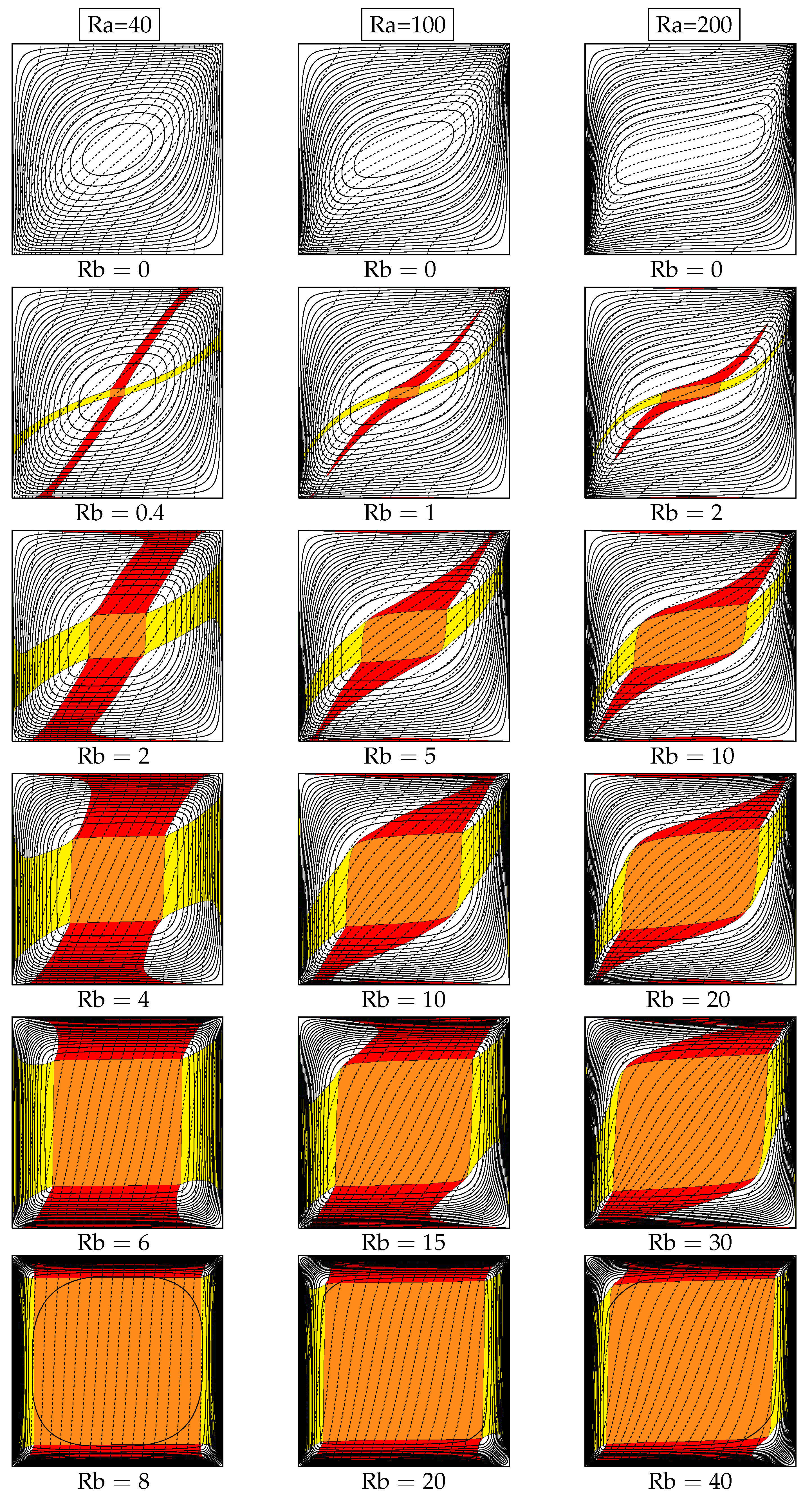
Figure 1 shows the streamlines and isotherms for a representative selection of values of and . Three different values of are considered, , 100 and 200, and each row of frames that corresponds is characterised by having identical values of . The continuous lines are the streamlines, while the dotted lines correspond to the isotherms. In all cases there is a clockwise circulation due to the fact that the left-hand boundary is heated. The shaded regions indicate the three different types of stagnation that exist. The red regions correspond to vertical stagnation, and therefore, the flow is purely horizontal along the horizontal channels. On the other hand, the yellow regions display where there is horizontal stagnation, and hence, the flow is purely vertical. We refer to these red and yellow regions as being semi-stagnant in order to distinguish them from the orange regions, which are fully stagnant.
The uppermost row of frames shows the streamfunction and temperature fields when the fluid is Newtonian (). The circulation is quite strong even when and it increases in strength as increases. This increasing strength is accompanied by an increasing deformation of the isotherms away from being vertical (when , for which ) towards the horizontal. We also note the very intense boundary layer formation on the sidewalls when , as evidenced by the tightly packed streamlines.
The second row of frames corresponds to when and this might be said to be a weakly plastic flow since the influence of a yield threshold is small. In one sense the pattern of the stagnant and semi-stagnant regions is not a surprise because they are placed about the loci where the streamlines for have vertical or horizontal tangents. Such semi-stagnant regions do not have counterparts when the Darcy–Bingham equations are isotropic (see [10]). However, the fully stagnant regions occupy a small region in the centre of the cavity, and the only difference between the present flows and the analogous flows in [10] is in the detailed shape of the stagnant region.
As the value of increases on the successive rows in Figure 1, the regions of semi-stagnation and full stagnation continue to increase in size. The yield threshold is becoming stronger relative to buoyancy, and thus the circulation weakens and the rate of heat transfer across the cavity decreases. The latter may be deduced from the fact that the isotherms are tending back towards being vertical. This is particularly noticeable in the last row of frames for which . In this case, the flow is essentially confined to a racetrack along edges of the cavity. Most of the circulation itself takes place either in the vertical or the horizontal direction, i.e., in regions of semi-stagnation, while the fluid changes direction in relatively small regions near the corners. For this type of microstructure, we may state unequivocally that the whole cavity becomes fully stagnant once . A different viewpoint is that, for a given value of (i.e., for a given fluid), buoyancy forces become strong enough to overcome the yield threshold once has risen to . These statements are based on the network model described in detail in [8], where the factor, 4, arises because it is the length of the perimeter of the cavity.
Figure 2 shows the effect of having different aspect ratios on the flow and temperature profiles for the case and . All four aspect ratios display a moderately large stagnation region in the centres of the respective cavities, but it is interesting to note that the red semi-stagnant regions decrease in thickness as the aspect ratio increases. Thus, the case is closer to being in a state of full stagnation than all of the other cases, and it is worth predicting at what aspect ratio one would obtain full stagnation. While the network analysis [8] does not cover anything other than a unit aspect ratio cavity, it is clear from that analysis that incipient stagnation arises when
where the right hand side is, once more, the perimeter of the cavity. The perimeter plays such a prominent role in the network model of Rees [8] because the buoyancy forces induced along the sidewalls must be sufficiently large to enable fluid to travel all the way around the channels that are on the boundary but not strong enough to cause it to travel along the next innermost set of channels just inside the boundary. Therefore, for the choice of and represented in Figure 2, namely, and , the cavity will be stagnant when .
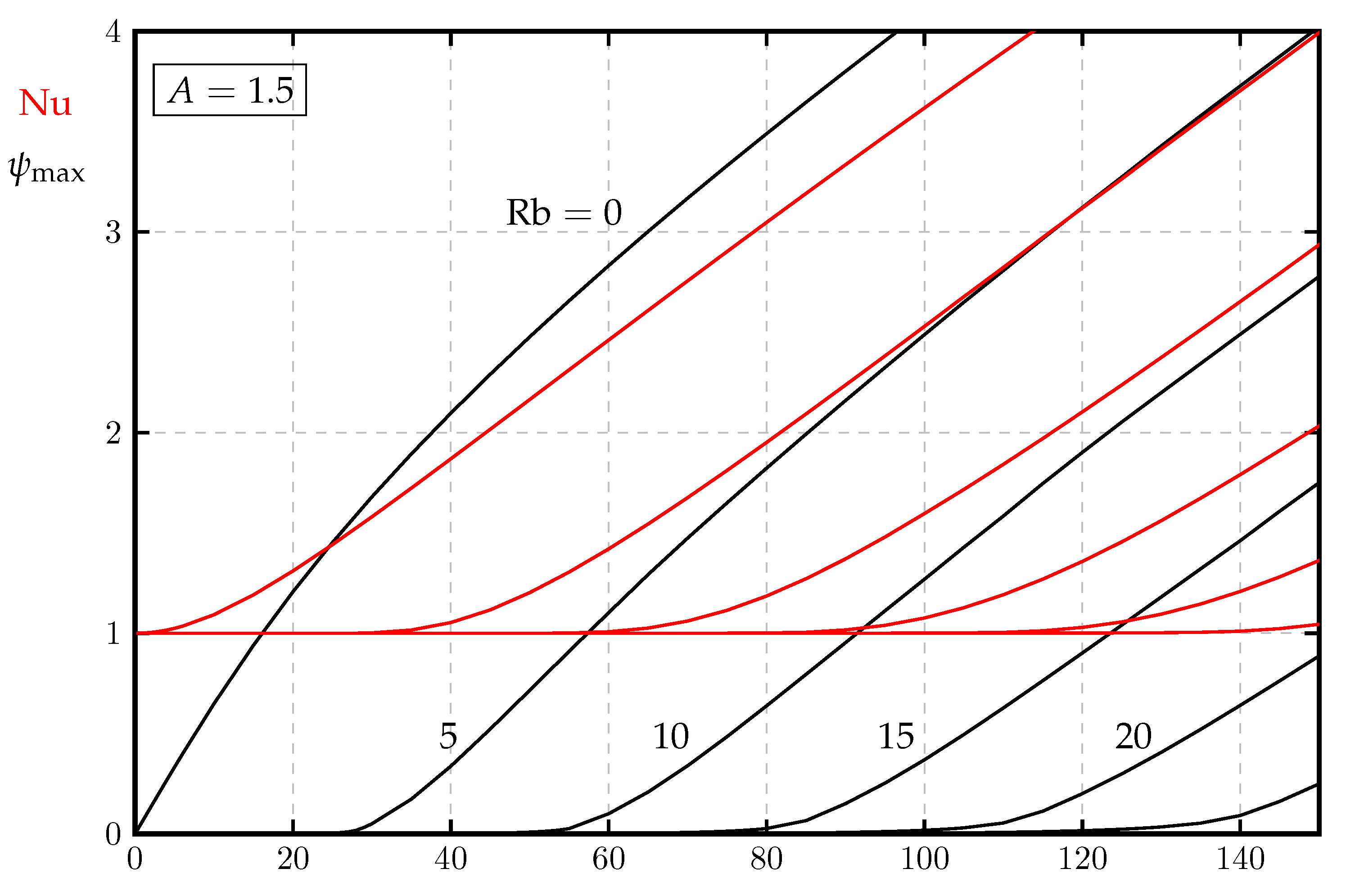
Figure 3, Figure 4, Figure 5 and Figure 6 show how that maximum value of the streamfunction and the Nusselt number vary with for a range of values of and for four different aspect ratios. Given the symmetry of the cavity and the governing equations, the maximum value of is the value at the centre of the cavity. The Nusselt number is defined as
where the derivative was approximated using a second-order accurate formula and the integration used the trapezium rule. The reason for the scaling (A) was to ensure that for the conductive state for all aspect ratios.
It is important to note that the curves shown in Figure 3, Figure 4, Figure 5 and Figure 6 have been processed to eliminate as much as is possible the effects of the weak flow that exists for relatively small values of due to the use of the regularisation; see Appendix B for details of how this was achieved.
5. Conclusions
We have computed the effects of having a porous microstructure consisting of horizontal and vertical channels on the patterns of convection in a sidewall-heated porous cavity where a Bingham fluid saturates the pores. The macroscopic governing equations were derived briefly, and the numerical method was described in some detail. In particular, the main difficulties associated with a parameter set that is close to the onset of convection were considered in detail in Appendix A. While the resulting computations yield clear streamline and isotherm contours, the accurate evaluation of the maximum value of the streamfunction, , and the Nusselt number, , required a Richardson extrapolation-like process between two solutions using different values of the regularisation constant in order to emulate Pascal’s law solution much more closely.
In general, it was found that convection, when it arises, splits the cavity into nine regions: one with full stagnation, two each with either vertical stagnation (i.e., purely horizontal motion) or horizontal stagnation (i.e., purely vertical motion), and four where the fluid is fully non-stagnant. Our numerical simulations have verified the network model of Rees [8], which states that convection occurs only when for a unit-aspect-ratio cavity. The simulations have also confirmed the more general result, , for a cavity with aspect ratio, A, for which is the perimeter.
Funding
This research received no external funding.
Data Availability Statement
Not acceptable.
Conflicts of Interest
The author declares no conflict of interest.
Nomenclature
| Latin letters | |
| A | aspect ratio of the cavity |
| C | specific heat |
| c | regularisation parameter |
| f | function of the scaled body force |
| the negative of the pressure gradient | |
| g | gravity |
| H | distance between the neighbouring channels centerlines |
| h | channel width |
| K | permeability |
| L | height of the cavity |
| Nu | Nusselt number |
| p | pressure |
| Darcy–Rayleigh number | |
| Rees–Bingham number | |
| T | temperature |
| u | horizontal Darcy velocity |
| w | vertical Darcy velocity |
| x | horizontal coordinate |
| z | vertical coordinate |
| Greek letters | |
| thermal diffusivity | |
| coefficient of cubical expansion | |
| temperature difference | |
| dimensionless temperature | |
| dynamic viscosity | |
| density | |
| the ratio of the pressure gradient to its threshold value | |
| porosity | |
| streamfunction | |
| Other symbols | |
| c | cold boundary |
| h | hot boundary |
| ref | reference value |
| x, z | partial derivatives with respect to x and z, respectively |
Appendix A. The Approach to Stagnation: A Numerical Assessment for Suitable Values of c
In this Appendix, we demonstrate the difficulty in obtaining accurate solutions in terms of the streamlines when the flow is weak, i.e., when is only just above its critical value for the chosen value of or, equivalently, when is just below that value when the flow ceases for a given value of . We have chosen to use the case, and , for a square cavity with a grid, and for a selection of values of the regularisation parameter, c. This is a finer grid than those which are often used used elsewhere, and it was chosen in order to be able to increase the value of c to much larger values.
Figure A1 shows four such cases with , , and in turn. When , the streamlines are very clearly in error because they resemble a low- flow of a Newtonian fluid. Our chosen method for determining the regions of semi-stagnation and stagnation is also in error because a large number of streamlines appear in what should be a stagnant region in most of the cavity. Another problem lies with the fact that any two adjacent semi-stagnant regions do not admit flow between them, which is unphysical. Ideally, we should be reproducing the qualitative results that were found in the network model of Rees [8], namely that flow is confined solely to a narrow track around the edge of the cavity.
Figure A1.
Streamlines (continuous) and isotherms (dashed) for the case , and using the following values of c: 100, 200, 800 and 1600.
Figure A1.
Streamlines (continuous) and isotherms (dashed) for the case , and using the following values of c: 100, 200, 800 and 1600.

When the regularisation constant is increased to the shapes of the semi-stagnant regions now assume a physically realistic form. Fluid moves around the edge of the cavity and predominantly within semi-stagnant regions but also within small nonstagnant regions at the four corners. However, there remains quite a large number of streamlines occupying what has been deemed the stagnant region. A four-fold increase in c to greatly reduces the number of streamlines in the stagnant zone, while a further doubling to removes all but one streamline from the stagnant zone. For this parameter set (, ) this last case is beginning to exhibit’ convergence difficulties. A further clearing out of the stagnant zone will require a larger value of c but a finer grid will be essential in order to be able to iterate towards that solution.
Finally, we note that incipient flow is, perhaps, one of the more important aspects of a Bingham fluid problem, and extraordinary lengths are needed in order to model this well. On the other hand, when the fluid is flowing freely (e.g., the rest of the paper) such extreme care does not need to be taken. Thus, the use of in Figure 1 and Figure 2 was sufficient for the fully stagnant zones to be clear of streamlines apart from the final row in Figure 1, which corresponds to weak flow.
Appendix B. Processing of the Numerical Data
The tanh-regularisation has enabled us to compute flows that correspond to the Pascal model of a Bingham fluid in a porous medium. When the Darcy–Rayleigh number is well above its critical value, the fluid flows strongly in much of the cavity, and the regions of semi-stagnation and full stagnation are relatively small. The numerical solutions are also quite accurate. A faithful simulation of the Pascal model would correspond to and as decreases from above towards the critical value. However, the tanh-regularisation softens this approach and, when is below its critical value, the large values of c that we have mean that and satisfy the following asymptotic relations,
for a fixed value of . Therefore, we are able to ‘clean up’ the variations of and with by using solutions with two different values of c.
If we declare to be the value of for a chosen value of c, then we are able to almost eliminate the presence of the regularisation-induced linear regime at subcritical values of by using the following formula (which is very reminscent of Richardson’s Extrapolation method):
Likewise, we processed the Nusselt number according to,
An example of the use of these formulae are shown in Figure A2, which depicts the case and where the variations of Q and with are shown (i) for , (ii) for and (iii) in the extrapolated forms calculated using Equations (A2) and (A3). For reference, the critical value of the Darcy–Rayleigh number is 50 for this aspect ratio and value of ; see Equation (25).
Figure A2.
For the aspect ratio, , the variation with of the maximum value of the streamfunction (black) and the Nusselt number, Nu (red) as . Continuous lines correspond to and dashed lines to . The green lines correspond to the respective extrapolates.
Figure A2.
For the aspect ratio, , the variation with of the maximum value of the streamfunction (black) and the Nusselt number, Nu (red) as . Continuous lines correspond to and dashed lines to . The green lines correspond to the respective extrapolates.

The presumed linear dependence of Q on is shown to be correct since the extrapolated form given by Equation (A2) is indistinguishable from the horizontal axis for subcritical values of . It is interesting to contrast the linear variation of and at subcritical values of , which is consistent with a Newtonian flow, and the quadratic variation of Q just above , which is characteristic of the Bingham fluid flow. On the other hand, there is very little difference between the three curves for .
References
- Pascal, H. Influence du gradient de seuil sur des essais de remontée de pression et d’écoulement dans les puits. Oil Gas Sci. Technol. 1979, 343, 87–404. [Google Scholar] [CrossRef]
- Bourgeat, A.; Mikelić, A. A note on homogenization of Bingham flow through a porous medium. J. Math. Pures Appl. 1993, 72, 405–414. [Google Scholar]
- Chevalier, T.; Chevalier, C.; Clain, X.; Dupla, J.C.; Canou, J.; Rodts, S.; Coussot, P. Darcy’s law for yield stress fluid flowing through a porous medium. J. Non-Newton. Fluid Mech. 2013, 195, 57–66. [Google Scholar] [CrossRef]
- Chevalier, T.; Talon, L. Generalization of Darcy’s law for Bingham fluids to porous media: From flow-field statistics to the flow-rate regimes. Phys. Rev. E 2015, 91, 023011. [Google Scholar] [CrossRef] [Green Version]
- Nash, S.; Rees, D.A.S. The effect of microstructure on models for the flow of a Bingham fluid in porous media. Transp. Porous Media 2017, 116, 1073–1092. [Google Scholar] [CrossRef] [Green Version]
- Bauer, D.; Talon, L.; Peysson, Y.; Ly, H.B.; Batôt, G.; Chevalier, T.; Fleury, M. Experimental and numerical determination of Darcy’s lawfor yield stress fluids in porous media. Phys. Rev. Fluids 2019, 4, 063301. [Google Scholar] [CrossRef]
- Liu, C.; De Luca, A.; Rosso, A.; Talon, L. Darcy’s Law for Yield Stress Fluids. Phys. Rev. Lett. 2019, 122, 245502. [Google Scholar] [CrossRef] [PubMed] [Green Version]
- Rees, D.A.S. Convection of a Bingham fluid in a porous medium. In Handbook of Porous Media; Vafai, K., Ed.; CRC Press/Taylor & Francis Group: Boca Raton, FL, USA, 2015; Chapter 17. [Google Scholar] [CrossRef]
- Rees, D.A.S. Two-dimensional flow of a Bingham fluid in a network model of a porous medium: The quest for isotropy. Paper in preparation.
- Rees, D.A.S. The convection of a Bingham fluid in a differentially-heated porous cavity. Int. J. Numer. Methods Heat Fluid Flow 2016, 26, 879–896. [Google Scholar] [CrossRef] [Green Version]
- Rees, D.A.S. Convective flow of Bingham fluids in internally-heated porous cavities. Comput. Therm. Sci. 2021, 13, 1–13. [Google Scholar] [CrossRef]
- Rees, D.A.S. Darcy-Bénard-Bingham convection. Phys. Fluids 2020, 32, 084107. [Google Scholar] [CrossRef]
- Rees, D.A.S. Nonlinear Wooding-Bingham convection. In Proceedings of the 11th International Conference on Computational Heat Mass and Momentum Transfer (ICCHMT18), Kraków, Poland, 21–24 May 2018. [Google Scholar]
- Buckingham, E. On Plastic Flow through Capillary Tubes. Proceed. Am. Soc. Test. Mater. 1921, 21, 1154–1156. [Google Scholar]
- Reiner, M. Ueber die Strömung einer elastischen Flüssigkeit durch eine Kapillare. Beitrag zur Theorie Viskositätsmessungen. Colloid Polym. Sci. 1926, 39, 80–87. [Google Scholar]
- Papanastasiou, T.C. Flow of materials with yield. J. Rheol. 1987, 31, 385–404. [Google Scholar] [CrossRef]
- Gill, A.E. A proof that convection in a porous vertical slab is stable. J. Fluid Mech. 1969, 35, 545–547. [Google Scholar] [CrossRef]
- Straughan, B. A nonlinear analysis of convection in a porous vertical slab. Geophys. Astrophys. Fluid Dyn. 1988, 42, 269–275. [Google Scholar] [CrossRef]
- Lewis, S.; Bassom, A.P.; Rees, D.A.S. The stability of vertical thermal boundary layer flow in a porous medium. Eur. J. Mech. B Fluids 1995, 14, 395–408. [Google Scholar]
- Rees, D.A.S. Comments on: “Heat transfer in a square porous cavity in presence of square solid block”. Int. J. Numer. Methods Heat Fluid Flow 2020, 30, 701–723. [Google Scholar] [CrossRef]
Figure 1.
Streamlines (continuous) and isotherms (dashed) using a square-network-based anisotropic model and with the given parameters. Red indicates vertical stagnation, yellow for horizontal stagnation and orange for total stagnation. Ra is the Darcy–Rayleigh number and Rb is the the Rees–Bingham number.

Figure 2.
Streamlines (continuous) and isotherms (dashed) using a square-network-based anisotropic model and showing the effect of having different cavity aspect ratios when and .
Figure 2.
Streamlines (continuous) and isotherms (dashed) using a square-network-based anisotropic model and showing the effect of having different cavity aspect ratios when and .

Figure 3.
For an aspect ratio, , the variation with of the maximum value of the streamfunction, (black) and the Nusselt number, Nu (red) as increases in steps of 5 from to . increases towards the right for and downwards for .
Figure 3.
For an aspect ratio, , the variation with of the maximum value of the streamfunction, (black) and the Nusselt number, Nu (red) as increases in steps of 5 from to . increases towards the right for and downwards for .

Figure 4.
For an aspect ratio, , the variation with of (black) and the Nusselt number, Nu (red) as increases in steps of 5 from to . increases towards the right for and downwards for .
Figure 4.
For an aspect ratio, , the variation with of (black) and the Nusselt number, Nu (red) as increases in steps of 5 from to . increases towards the right for and downwards for .

Figure 5.
For an aspect ratio, , the variation with of (black) and the Nusselt number, Nu (red) as increases in steps of 5 from to . increases towards the right for and downwards for .
Figure 5.
For an aspect ratio, , the variation with of (black) and the Nusselt number, Nu (red) as increases in steps of 5 from to . increases towards the right for and downwards for .

Figure 6.
For an aspect ratio, , the variation with of (black) and the Nusselt number, Nu (red) as increases in steps of 5 from to . increases towards the right for and downwards for .
Figure 6.
For an aspect ratio, , the variation with of (black) and the Nusselt number, Nu (red) as increases in steps of 5 from to . increases towards the right for and downwards for .

Publisher’s Note: MDPI stays neutral with regard to jurisdictional claims in published maps and institutional affiliations. |
© 2022 by the author. Licensee MDPI, Basel, Switzerland. This article is an open access article distributed under the terms and conditions of the Creative Commons Attribution (CC BY) license (https://creativecommons.org/licenses/by/4.0/).
Share and Cite
MDPI and ACS Style
Rees, D.A.S. Free Convection of a Bingham Fluid in a Differentially-Heated Porous Cavity: The Effect of a Square Grid Microstructure. Physics 2022, 4, 202-216. https://0-doi-org.brum.beds.ac.uk/10.3390/physics4010015
AMA Style
Rees DAS. Free Convection of a Bingham Fluid in a Differentially-Heated Porous Cavity: The Effect of a Square Grid Microstructure. Physics. 2022; 4(1):202-216. https://0-doi-org.brum.beds.ac.uk/10.3390/physics4010015
Chicago/Turabian StyleRees, D. Andrew S. 2022. "Free Convection of a Bingham Fluid in a Differentially-Heated Porous Cavity: The Effect of a Square Grid Microstructure" Physics 4, no. 1: 202-216. https://0-doi-org.brum.beds.ac.uk/10.3390/physics4010015