Conduction–Radiation Coupling between Two Distant Solids Interacting in a Near-Field Regime


1
Laboratoire Charles Fabry, UMR 8501, Institut d’Optique, Centre National de la Recherche Scientifique (CNRS), Université Paris-Saclay, 2 Avenue Augustin Fresnel, 91127 Palaiseau, France
2
ColibrITD, 91, rue du Faubourg Saint-Honoré, 75008 Paris, France
*
Author to whom correspondence should be addressed.
Physics 2023, 5(3), 784-796; https://0-doi-org.brum.beds.ac.uk/10.3390/physics5030049
Submission received: 17 May 2023
/
Revised: 19 June 2023
/
Accepted: 27 June 2023
/
Published: 13 July 2023
(This article belongs to the Special Issue Matter-Radiation Interactions—In Memory of Professor Francesco Saverio Persico)
Abstract
:In the classical approach to dealing with near-field radiative heat exchange between two closely spaced bodies, no coupling between the different heat carriers inside the materials and thermal photons is usually considered. Here, we provide an overview of the current state of research on this coupling between solids of different sizes while paying specific attention to the impact of the conduction regime inside the solids on the conduction–radiation coupling. We describe how the shape of the solids affects this coupling, and show that it can be located at the origin of a drastic change in the temperature profiles inside each body and the heat flux exchanged between them. These results could have important implications in the fields of nanoscale thermal management, near-field solid-state cooling, and nanoscale energy conversion.
1. Introduction
Radiative heat transfer is the phenomenon through which two bodies at different temperatures can exchange energy even when separated by vacuum. A milestone in the study of this effect, dating back to the 19th century, is Stefan–Boltzmann’s law, setting an upper bound for the flux two bodies at temperatures and can exchange; this upper limit, equal to , being the Stefan–Boltzmann constant, can be realized only in the ideal scenario of two black bodies (i.e., bodies absorbing all incoming radiation) exchanging heat. A second breakthrough in the study of radiative heat transfer was set much later, in the 1970s, with the development of fluctuational electrodynamics through the pioneering works of Rytov, Polder, and van Hove [1,2]. This theoretical framework describes each body as a collection of fluctuating dipoles with statistical properties that depend, by means of the fluctuation–dissipation theorem, on the temperature and optical properties of the body they belong to. This theory shed light on the very first experimental results [3] demonstrating the possibility of exceeding the blackbody limit in near-field regime, i.e., when the separation distance, d, between the solids is small compared to the thermal wavelength, (with ℏ the reduced Planck’s constant, c the speed of light, and the Boltzmann constant), which is on the order of 10m at ambient temperature. More specifically, this is prone to happening when the two bodies support resonant modes of the electromagnetic field, such as phonon-polaritons (for polar materials), plasmons (for metals) [4], or even a continuum of evanescent modes, such as hyperbolic modes [5]. The main reason underlying flux amplification in the presence of resonant modes is the fact that for these modes the field is confined to the interface between each material and the vacuum, and decays exponentially along the direction perpendicular to the interface. As a consequence, while the confined photons cannot contribute to the energy transfer when the two bodies are far from each other, they are able to tunnel between them when the distance is small enough, representing an additional channel for energy flux [6,7]. Thus far, this physical analysis neglects the role of the two temperatures. In fact, however, the latter play a major role in dictating the frequencies, , of the field modes participating in energy flux via the Bose–Einstein factor, . This explains why near-field flux amplification is typically much stronger for polar materials than for metals, the reason being that for the former (latter), the asymptotic value of the resonant-mode dispersion relation typically lies in the infrared (ultraviolet) region of the spectrum, and can (cannot) be excited at ambient temperature.
The unveiling of near-field flux amplification paved the way for numerous subsequent experiments in a variety of geometries (see the reviews in Refs. [8,9,10] for more details), including, plane–plane, sphere–plane, and tip–plane, as well as for several different materials. Parallel to these experimental investigations, several ideas for applications have been put forward, ranging from energy conversion devices [11,12,13,14] to heat-assisted data recording [15,16], infrared spectroscopy [17,18], and thermotronics [19,20], that is, the concept of thermal equivalents of electrical circuit elements.
Although the vast majority of experiments have confirmed the theoretical predictions, a few have observed deviations, both in the extreme near-field scenario [21] (nanometer and sub-nanometer range of distances) and at tens of nanometers [22,23]. More specifically, an amplification of the flux was observed in Ref. [21], whereas a saturation effect was highlighted in Refs. [22,23]. The explanation for such inconsistencies between theory and experiment, which are unsolved as yet, has stimulated theoretical investigations in several directions. First, it has been suggested that non-local effects must be taken into account in order to describe the energy exchange between metals at short separation distances [24,25]. Moreover, in the extreme near field, the participation of other heat carriers (phonons and electrons) could affect significantly the exchanged flux [26,27,28,29,30,31,32,33,34]; however, these can only play a role below a few nanometers. Finally, in this sense, a few studies have explored the transition between conduction and radiation [35,36].
A further effect which could be at the origin of a deviation with respect to the predictions of fluctuational electrodynamics is the coupling between conduction acting inside each body and near-field radiative heat transfer between them. In order to understand the possible impact of this effect, we can visualize a typical theoretical system as shown in Figure 1. Two bodies are kept at temperatures and by two thermostats locally connected to them. In almost all theoretical works on near-field radiative heat transfer, it is assumed that conduction inside each body is efficient enough (compared to the energy exchange mediated by radiation) that the temperature can be assumed to be uniform in each body and equal to that imposed by the thermostat. This allows the radiative heat transfer between two bodies at two given temperatures, and , to be properly defined. Nevertheless, the strong dependence of near-field radiative heat transfer on the materials involved, and more importantly on the separation distance, suggests that these two effects could compete in certain ranges of parameters. This would imply the existence of a temperature profile within each body (as depicted in Figure 1), and in turn a modification of the flux exchanged through radiation.
Over the past several years we have performed a comprehensive study of the impact of this coupling [37,38,39,40,41,42,43], which is the topic of the present review paper. More specifically, we first studied this effect in the convenient geometry of two parallel slabs and in the diffusive regime, as discussed in Section 2. Following this first analysis, we investigated the role played by the size of the two bodies. As a matter of fact, as shown pictorially in Figure 1, this can have an impact on the conduction transport regime inside each body. These results are discussed in Section 3. Finally, in order to account for the variety of geometries employed in experiments, we studied the same coupling effect in different geometries, as discussed in Section 4. Our conclusions on the basis of these studies are provided in Section 5.
2. Slab–Slab Configuration in the Diffusive Conduction Regime
The simplest geometry to study the effect of conduction–radiation coupling is that involving two parallel slabs with finite thickness separated by a vacuum gap of thickness d, as represented in the inset of Figure 2. To describe the action of two thermostats connected to the two bodies, we assume that the temperature in the first (second) body is fixed at () except over a region of thickness ().
In order to further simplify the problem, we assume that the thickness of the two slabs is sufficient to safely treat the conduction problem in the Fourier diffusive regime. In this case, the coupled equation to be solved reads:
In Equation (1), is the bulk Fourier conductivity at point z, whereas represents the radiative power per unit volume emitted at a point and absorbed at a point z. At this stage, the expression of the radiative term is needed. This energy exchange can be calculated by means of a framework introduced to calculate both Casimir forces and radiative heat transfer, and is based on the knowledge of the scattering operators of the bodies involved [44,45,46,47]. In order to account for the temperature profiles, we assume that each body is divided into slabs of infinitesimal thickness, for which the scattering coefficients are known analytically, and apply the scattering approach to deduce the radiative heat transfer. Limiting ourselves to the contribution stemming from evanescent waves in transverse magnetic polarization (which dominates in the near field between polar materials [4]), we can write the flux as the frequency and wavevector integral, (see [38] for more details), where the spectral flux can be expressed as
where is the parallel -component of the wavevector and and are the perpendicular components in the vacuum and inside the slabs, respectively. We introduce the Fresnel reflection coefficient of a slab, provided by . Finally, in Equation (2), the notation represents the imaginary part of a.
The coupled heat Equation (1) can be combined with the flux expression (2), allowing it to be solved numerically. Nevertheless, two further approximations can be performed that allow us to obtain an analytical expression for both the temperature gap between the two slabs (across the vacuum gap; see Figure 2) and the exchanged flux. We can first assume that the radiative energy exchange takes place over a tiny thickness close to the vacuum interface of each body, allowing us to treat it as a surface term, i.e., as a boundary condition. Moreover, inspired by the results of fluctuational electrodynamics, we can assume that the total flux exchanged radiatively can be expressed as , where denotes the radiative thermal conductance of the system. In this simplified expression, the flux depends only on the two temperatures at the interfaces, and shows the known divergence. These approximations, their validity having been numerically verified, lead to the following analytical solutions:
The impact of conduction–radiation coupling is shown quantitatively in Figure 2 and Figure 3. Figure 2 concerns two silica slabs with m and K. The temperature profile is shown inside the left slab for three different distances, showing that the temperature can decrease by more than 100 K in the left slab for the smallest distance considered. Moreover, the inset of Figure 2, showing the numerically-calculated distribution of flux absorbed inside the slab, indicates that it has a high peak around the vacuum interface, confirming the previous assumption.
Figure 3 shows the temperature difference across the gap (normalized with respect to ; see inset) and the exchanged flux (main part) for different slab thicknesses (see caption of Figure 3). It can be well observed that in addition to the temperature profile being induced by the coupling (an effect that grows with the slab thickness), the flux is strongly modified with respect to the scenario of absence of coupling (the orange dashed line in Figure 3). The flux tends to be saturated for d going to zero, and both the saturation value and the characteristic distance at which the distance-dependent flux deviates from the no-coupling scenario depend strongly on the thickness.
In order to make this example more quantitative, it is interesting to define a characteristic coupling distance such that, at this distance, the temperature gradient across the vacuum gap equals half of . At this distance, we have: and . The distance, , depends on both the thickness and on the material-dependent parameter, quantifying the competition between radiative exchange (through ) and conductive transport (through the conductivity ). Figure 4 shows as a function of this ratio for m. On top of this curve, we highlight a few examples of different materials, showing that this characteristic distance can vary from just a few to tens or hundreds of nanometers, making the experimental observation of conduction–radiation coupling in principle feasible for certain materials and thicknesses. We conclude this section by mentioning that a previous study was performed in this same sense [48], though it applied only to a specific configuration and did not explore the strong dependence on the choice of materials and thicknesses.
3. The Impact of Slab Thickness: From the Diffusive to the Ballistic Regime
The results presented in Section 2 are based on the assumption that the thickness of the two bodies exchanging heat is large compared to the mean free path of the phonons inside them, i.e., in the micron range for typical polar materials. Nevertheless, because of the peculiar transport regimes, which can arise for conduction depending on the thickness, we have extended our study to the more general configuration of arbitrary thickness. While atomistic approaches can be exploited to describe heat transport at the nanoscale in arbitrary transport regimes (see [49] and references therein), we have employed a mesoscopic approach here. Boltzmann’s transport equation is the mathematical tool allowing us to fully grasp the transition between the transport regimes, and more specifically between the two extreme ones, namely, ballistic and diffusion regimes. While in certain regimes (e.g., Fourier conductive transport) this coupling could be described in simpler terms, using for example effective descriptions of the heat transport channels, a fully coupled approach such as the one described below is necessary to unveil the full behavior of radiation–conduction coupling for arbitrary thicknesses and distances.
At a given frequency (not explicitly shown) and in the relaxation time approximation, this equation reads:
The unknown of this equation is the distribution function, , associated with the heat carriers within the solid for each polarization p, at time t, solid angle , and position . Moreover, is the group velocity of carriers at polarization p and frequency , is the equilibrium distribution (Fermi–Dirac for electrons and Bose-Einstein for phonons), and is the heat-carrier relaxation time.
In order to solve Equation (4), it has to be coupled to the equation governing the time evolution of the internal energy density, u, which reads:
Here, denotes the radiative power locally dissipated per unit volume within a given body that comes from the other body, which can be calculated using a fluctuational electrodynamics approach (see [37] for more details). denotes the conductive power per unit volume at position , equal to the divergence of the conductive flux, , which is connected to the distribution function, , through the relation,
with representing the density of the states.
We solve the two coupled equations in the geometry of two parallel SiC slabs (analogous to the one shown in Figure 1): the left one, denoted by index 1, is connected to a thermostat at temperature K, whereas slab 2 on the right is connected to a thermostat at K. Concerning the boundary conditions, two different cases must be taken into account: for the edges in contact with the vacuum, phonons hitting the surface are scattered specularly (specular reflection), whereas phonons colliding with the thermostat are scattered in all directions (diffuse reflection) [50]. By exploiting Boltzmann’s equation, we are able to let the slab thickness vary in a wide range of values, from the ballistic to the diffusive regime.
The results at two separation distances ( and nm) are shown in Figure 5. The main part of the two plots shows the temperature profile inside slab 1 normalized to the temperature difference, , across it. This allows a signature of the conductive transport regime to be highlighted in the shape of the temperature profile. More specifically, while for the largest thickness considered here, becomes almost linear (as it should be in the strictly diffusive regime according to Fourier’s law), with decreasing thickness a transition is observed towards a significantly different behavior. In this ballistic-like scenario, the temperature profile tends towards a uniform distribution, excluding the region close to the thermostat () where is almost discontinuous (Casimir regime) and close to the vacuum gap, where shows a steep increase; this is physically linked to the fact that most of the radiative flux is absorbed close to the boundary.
While this discussion highlights the impact of the transport regime on the shape of the temperature profile, the information regarding the quantitative impact of distance and thickness is contained in the insets of Figure 5. It is clear that an observable temperature profile (up to tens of degrees) can indeed arise, mainly for large thicknesses (tens of microns) and small distances (below 5 nm).
Figure 6 addresses the impact of the temperature profiles on the exchange radiative flux. The exact result (solid black line) is compared to two approximate configurations, namely, the Polder and van Hove result (i.e., conventional fluctuational electrodynamics ignoring the existence of a temperature profile, red dashed line) and the modified Polder and van Hove configuration (the blue long-dashed line). The latter corresponds to a conventional fluctuational electrodynamics configuration, with the assumption that the temperature inside each body is uniform and equal to the temperature at the boundary between it and the vacuum.
As these curves show, at the closest distance nm the error when using standard fluctuational electrodynamics (ignoring conduction–radiation coupling) can be enormous, revealing once more the relevance of the coupling effect for large thicknesses and small distances. On the contrary, the modified approach reproduces the exact result relatively well. On the one hand, this confirms that radiative heat transfer is mainly a surface effect that depends almost entirely on the temperature at the boundaries between each body and the vacuum. Nevertheless, though it is of fundamental interest, this has no direct practical use as the knowledge of these boundary temperatures stems from and requires the solution to the full problem in the presence of coupling. Apart from being relevant for comparing theory and experiment, these coupling effects could be relevant in certain applications involving e.g., the thermalization of two bodies, as discussed in detail in Ref. [42].
4. The Impact of Geometry: The Tip–Plane Configuration
After investigating the role played by the thicknesses of the two bodies, it is interesting to address the impact of the geometrical configuration, both to unveil possible fundamental issues and because experiments are only rarely performed in the plane–plane configuration, as it raises the significant experimental challenge of ensuring parallelism.
In a preliminary study [41], we investigated conduction–radiation coupling between two nanorods. In this configuration, we highlighted, the appearance of a temperature profile, in turn modifying the exchanged radiative flux, along with a deviation from a linear temperature profile, even in the diffusive regime, due to the appearance of bulk polaritonic resonances that are absent in the case of two parallel planes.
Here, we focus in detail more on a recent study [43] where we analyzed the effect of conduction–radiation coupling in the tip–plane scenario, which is more frequently employed in experiments (see, e.g., Ref. [51]). While this configuration is often described theoretically by means of a sphere–plane configuration, we used a different approach and considered the geometrical configuration sketched in Figure 7, where two cylinders of radius and , where f is radii fraction, are placed in front of each other and separated by a vacuum gap with thickness d. The former (latter) has thickness (), and is connected to a thermostat at temperature (). Modulation of the factor f allows switching from the plane–plane configuration () to a tip–plane scenario, in which f tends to zero.
Inspired by the results discussed in Section 3, we can consider large values for the two thicknesses (m) such that we are in the diffusive regime. We then solve the heat equation in cylindrical coordinates. To this end, we exploit the Derjaguin approximation [52] (known as proximity-force approximation), typically employed to describe energy and momentum fluxes in complex geometries such as a sphere and a plane. This approximation is based on a decomposition of two facing bodies in pairs of small planar elements facing each other, to which the known result for two parallel planes is applied. In our scenario, this is equivalent to assuming that the two cylinders do not exchange any flux across their lateral surfaces and that they exchange heat radiatively only across the surface of the smaller cylinder. In other words, for the left cylinder, we have: for , while for both cylinders, we have for . The solution can be obtained analytically under the further approximation that the exchanged flux can be written as
i.e., it is uniform, depending only on the two temperatures at the center of the two cylinder surfaces and on the separation distance as . Here, denotes the radiative thermal conductance of the system. This allows the analytical expression for the temperature profiles in the cylinders to be obtained as follows:
where is the nth-order Bessel function of the first kind and () is the set of zeros of , and for the exchanged radiative flux as follows:
with () being the height of the larger (smaller) cylinder. In these expressions, we define
As expected, Equation (9) allows us to recover the results for two parallel slabs [38] for . As discussed in more detail in Ref. [43], moving beyond the approximation described in Equation (7) allows us to obtain numerical results that are in a good enough agreement with the analytical expressions for the physical parameters taken into account below.
The results for a configuration with m, m, and are shown in Figure 8a, where these results are compared to the configuration with no coupling and to the slab–slab scenario (corresponding to ).
More specifically, Figure 8a shows the results for silica (SiO), silicon carbide (SiC), and gold bodies. In the latter scenario, it can be observed that for both slabs and cylinders the curves in the absence and presence of coupling are indistinguishable. The reason for this is that the radiative exchange in the case of gold is weak compared to the case of polar materials, mainly because the asymptotic value of the surface-resonant-mode (surface plasmons) dispersion relation supported by gold lies in the ultraviolet region of the spectrum. This value of the frequency corresponds to a large number of wave vectors contributing to energy exchange close to a specific frequency, which can lead to the well-known almost monochromatic heat-flux amplification in the near field. Since this frequency is quite weakly excited thermally around ambient temperature, no significant temperature profile and no impact on the radiative flux are expected in the case of gold.
On the contrary, based on the discussion in Section 2, for two polar materials the radiative heat flux in the nanometer range of distances is supposed to compete with conduction. The results in Figure 8a show that the results for two cylinders qualitatively follow those for two slabs; the characteristic distance at which the curve in the presence of coupling deviates from the one in the absence of coupling is almost the same, while the value of the saturated () flux is only slightly higher than the result for two slabs. This allows us to state that in a tip–plane configuration the impact of conduction–radiation coupling should be observable, at least for polar materials, in the nanometer range of distances.
To conclude, in Figure 8b we analyze the combined effect of the radius, , and radii fraction, f. It can be observed that the ratio between the flux in the presence [] and absence [] of coupling is on the order of in a wide range of both parameters. Finally, the black dashed line in Figure 8b indicates that the flux correction is significant for all points defining a hypothetical tip radius of 100 nm, corresponding to an experimentally reasonable value.
5. Conclusions and Perspectives
In this paper, we have reviewed our recent studies on the coupling between conduction and radiation for two solids out of thermal equilibrium interacting in a near-field regime. We have shown that, depending on the separation distance and the materials nature under scrutiny, the coupling can be at the origin of a non-negligible temperature profile inside each body (ignored in previous investigations), which can in turn induce a saturation of the radiative heat flux exchanged in the two bodies with respect to the predictions of conventional fluctuational electrodynamics.
Thanks to the the current possibility of experimentally exploring distances in the nanometer range and below [21,53], along with the ongoing miniaturization of a variety of technological devices, the results presented here show that conduction–radiation coupling needs to be taken into account both for the sake of comparing theory and experiment and in view of the design of innovative devices operating at the nanoscale. In that sense, several open problems have to be faced. First, the development of a numerical code able to tackle the coupled heat problem in an arbitrary geometry would pave the way to more reliable, flexible, and predictive theoretical results. While such a numerical framework has been developed for radiative heat transfer (see, e.g., [54]), no such tool yet exists for the conduction–radiation problem. Another important yet neglected point is the possible existence of multiple simultaneous regimes for conductive heat transport. As a matter of fact, a shape such as a tip, allowing for a continuum of length scales, could imply a transition from ballistic to diffusive conductive heat transport, which could in turn induce interesting temperature profiles. Finally, conduction–radiation coupling could be studied in a many-body scenario [10], in which the intrinsic non-additive nature of radiative heat transfer could pave to way to promising methods of controlling heat transfer at the nanoscale.
Author Contributions
Conceptualization, P.B.-A. and R.M.; methodology, P.B.-A. and R.M.; software, M.R., C.G.A.B., P.B.-A. and R.M.; investigation, M.R., C.G.A.B., P.B.-A. and R.M.; formal analysis, M.R., C.G.A.B., P.B.-A. and R.M.; writing—original draft preparation, P.B.-A. and R.M.; writing—review and editing, M.R., C.G.A.B., P.B.-A. and R.M. All authors have read and agreed to the published version of the manuscript.
Funding
We acknowledge financial support from Labex Nanosaclay, ANR-10-LABX-0035 (Flagship project MaCaCQu), France.
Data Availability Statement
The data that support the findings of this study are available from the corresponding author upon reasonable request.
Conflicts of Interest
The authors declare no conflict of interest.
References
- Rytov, S.M.; Kravtsov, Y.A.; Tatarskii, V.I. Principles of Statistical Radiophysics: 3. Elements of Random Fields; Springer: Berlin/Heidelberg, Germany, 1989. [Google Scholar]
- Polder, D.; van Hove, M. Theory of radiative heat transfer between closely spaced bodies. Phys. Rev. B 1971, 4, 3303–3314. [Google Scholar] [CrossRef]
- Hargreaves, C.M. Anomalous radiative transfer between closely-spaced bodies. Phys. Lett. A 1969, 30, 491–492. [Google Scholar] [CrossRef]
- Joulain, K.; Mulet, J.-P.; Marquier, F.; Carminati, R.; Greffet, J.-J. Surface electromagnetic waves thermally excited: Radiative heat transfer, coherence properties and Casimir forces revisited in the near field. Surf. Sci. Rep. 2005, 57, 59–112. [Google Scholar] [CrossRef] [Green Version]
- Biehs, S.-A.; Tschikin, M.; Ben-Abdallah, P. Hyperbolic Metamaterials as an Analog of a Blackbody in the Near Field. Phys. Rev. Lett. 2012, 109, 104301. [Google Scholar] [CrossRef] [Green Version]
- Pendry, J.B. Radiative exchange of heat between nanostructures. J. Phys. Condens. Matt. 1999, 11, 6621–6633. [Google Scholar] [CrossRef]
- Volokitin, A.I.; Persson, B.N.J. Near-field radiative heat transfer and noncontact friction. Rev. Mod. Phys. 2007, 79, 1291–1329. [Google Scholar] [CrossRef]
- Song, B.; Fiorino, A.; Meyhofer, E.; Reddy, P. Near-field radiative thermal transport: From theory to experiment. AIP Adv. 2015, 5, 053503. [Google Scholar] [CrossRef] [Green Version]
- Cuevas, J.C.; García-Vidal, F.J. Radiative heat transfer. ACS Photonics 2018, 5, 3896–3915. [Google Scholar] [CrossRef]
- Biehs, S.-A.; Messina, R.; Venkataram, P.S.; Rodriguez, A.W.; Cuevas, J.C.; Ben-Abdallah, P. Near-field radiative heat transfer in many-body systems. Rev. Mod. Phys. 2021, 93, 025009. [Google Scholar] [CrossRef]
- DiMatteo, R.S.; Greiff, P.; Finberg, S.L.; Young-Waithe, K.A.; Choy, H.K.H.; Masaki, M.M.; Fonstad, C.G. Enhanced photogeneration of carriers in a semiconductor via coupling across a non isothermal nanoscale vacuum gap. Appl. Phys. Lett. 2001, 79, 1894–1896. [Google Scholar] [CrossRef]
- Narayanaswamy, A.; Chen, G. Surface modes for near field thermophotovoltaics. Appl. Phys. Lett. 2003, 82, 3544–3546. [Google Scholar] [CrossRef]
- Basu, S.; Chen, Y.-B.; Zhang, Z.M. Microscale radiation in thermophotovoltaic devices—A review. Int. J. Energy Res. 2007, 31, 689–716. [Google Scholar] [CrossRef]
- Fiorino, A.; Zhu, L.; Thompson, D.; Mittapally, R.; Reddy, P.; Meyhofer, E. Nanogap near-field thermophotovoltaics. Nat. Nanotech. 2018, 13, 806–811. [Google Scholar] [CrossRef]
- Challener, W.A.; Peng, C.; Itagi, A.V.; Karns, D.; Peng, W.; Peng, Y.; Yang, X.; Zhu, X.; Gokemeijer, N.J.; Hsia, Y.-T.; et al. Heat-assisted magnetic recording by a near-field transducer with efficient optical energy transfer. Nat. Photon. 2009, 3, 220–224. [Google Scholar] [CrossRef]
- Stipe, B.C.; Strand, T.C.; Poon, C.C.; Balamane, H.; Boone, T.D.; Katine, J.A.; Li, J.-L.; Rawat, V.; Nemoto, H.; Hirotsune, A.; et al. Magnetic recording at 1.5 Pb m−2 using an integrated plasmonic antenna. Nat. Photon. 2020, 4, 484–488. [Google Scholar] [CrossRef]
- De Wilde, Y.; Formanek, F.; Carminati, R.; Gralak, B.; Lemoine, P.-A.L.; Joulain, K.; Mulet, J.-P.; Chen, Y.; Greffet, J.-J. Thermal radiation scanning tunnelling microscopy. Nature 2006, 444, 740–743. [Google Scholar] [CrossRef] [PubMed]
- Jones, A.C.; Raschke, M.B. Thermal infrared near-field spectroscopy. Nano Lett. 2012, 12, 1475–1481. [Google Scholar] [CrossRef]
- Ben-Abdallah, P.; Biehs, S.-A. Near-Field Thermal Transistor. Phys. Rev. Lett. 2013, 112, 044301. [Google Scholar] [CrossRef] [PubMed] [Green Version]
- Ben-Abdallah, P.; Biehs, S.-A. Contactless heat flux control with photonic devices. AIP Adv. 2015, 5, 053502. [Google Scholar] [CrossRef]
- Kloppstech, K.; Könne, N.; Biehs, S.-A.; Rodriguez, A.W.; Worbes, L.; Hellmann, D.; Kittel, A. Giant heat transfer in the crossover regime between conduction and radiation. Nat. Commun. 2017, 8, 14475. [Google Scholar] [CrossRef] [Green Version]
- Kittel, A.; Müller-Hirsch, W.; Parisi, J.; Biehs, S.-A.; Reddig, D.; Holthaus, M. Near-field heat transfer in a scanning thermal microscope. Phys. Rev. Lett. 2005, 95, 224301. [Google Scholar] [CrossRef] [PubMed] [Green Version]
- Shen, S.; Narayanaswamy, A.; Chen, G. Surface phononpolaritons mediated energy transfer between nanoscale gaps. Nano Lett. 2009, 9, 2909–2913. [Google Scholar] [CrossRef] [PubMed]
- Ford, G.W.; Weber, W.H. Electromagnetic interactions of molecules with metal surfaces. Phys. Rep. 1984, 113, 195–287. [Google Scholar] [CrossRef] [Green Version]
- Chapuis, P.-O.; Volz, S.; Henkel, C.; Joulain, K.; Greffet, J.-J. Effects of spatial dispersion in near-field radiative heat transfer between two parallel metallic surfaces. Phys. Rev. B 2008, 77, 035431. [Google Scholar] [CrossRef] [Green Version]
- Zhang, Z.Q.; Lü, J.T.; Wang, J.S. Energy transfer between two vacuum-gapped metal plates: Coulomb fluctuations and electron tunneling. Phys. Rev. B 2018, 97, 195450. [Google Scholar] [CrossRef] [Green Version]
- Alkurdi, A.; Adessi, C.; Tabatabaei, F.; Li, S.; Termentzidis, K.; Merabia, S. Thermal transport across nanometre gaps: Phonon transmission vs. air conduction. Int. J. Heat Mass Transf. 2020, 158, 119963. [Google Scholar] [CrossRef]
- Volokitin, A.I. Effect of an electric field in the heat transfer between metals in the extreme near field. JETP Lett. 2019, 109, 749–754. [Google Scholar] [CrossRef]
- Volokitin, A.I. Contribution of the acoustic waves to near-field heat transfer. J. Phys. Condens. Matt. 2020, 32, 215001. [Google Scholar] [CrossRef] [PubMed] [Green Version]
- Volokitin, A.I. Electric double layer effect in an extreme near-field heat transfer between metal surfaces. Phys. Rev. B 2021, 103, L041403. [Google Scholar] [CrossRef]
- Tokunaga, T.; Jarzembski, A.; Shiga, T.; Park, K.; Francoeur, M. Extreme near-field heat transfer between gold surfaces. Phys. Rev. B 2021, 104, 125404. [Google Scholar] [CrossRef]
- Tokunaga, T.; Arai, M.; Kobayashi, K.; Hayami, W.; Suehara, S.; Shiga, T.; Park, K.; Francoeur, M. First-principles calculations of phonon transport across a vacuum gap. Phys. Rev. B 2022, 105, 045410. [Google Scholar] [CrossRef]
- Guo, Y.; Adessi, C.; Cobian, M.; Merabia, S. Atomistic simulation of phonon heat transport across metallic vacuum nanogaps. Phys. Rev. B 2022, 106, 085403. [Google Scholar] [CrossRef]
- Gómez Viloria, M.; Guo, Y.; Merabia, S.; Ben-Abdallah, P.; Messina, R. Role of the Nottingham effect in heat transfer in the extreme near-field regime. Phys. Rev. B 2023, 107, 125414. [Google Scholar] [CrossRef]
- Chiloyan, V.; Garg, J.; Esfarjani, K.; Chen, G. Transition from near-field thermal radiation to phonon heat conduction at subnanometre gaps. Nat. Commun. 2015, 6, 6775. [Google Scholar] [CrossRef] [Green Version]
- Joulain, K. Near-field heat transfer: A radiative interpretation of thermal conduction. J. Quant. Spectrosc. Radiat. Transf. 2008, 109, 294. [Google Scholar] [CrossRef]
- Reina, M.; Messina, R.; Ben-Abdallah, P. Conduction-radiation coupling between two closely-separated solids. Phys. Rev. Lett. 2021, 125, 224302. [Google Scholar] [CrossRef] [PubMed]
- Messina, R.; Jin, W.; Rodriguez, A.W. Strongly coupled near-field radiative and conductive heat transfer between planar bodies. Phys. Rev. B 2016, 94, 121410. [Google Scholar] [CrossRef] [Green Version]
- Messina, R.; Jin, W.; Rodriguez, A.W. Exact formulas for radiative heat transfer between planar bodies under arbitrary temperature profiles: Modified asymptotics and sign-flip transitions. Phys. Rev. B 2016, 94, 205438. [Google Scholar] [CrossRef] [Green Version]
- Jin, W.; Messina, R.; Rodriguez, A.W. Near-field radiative heat transfer under temperature gradients and conductive transfer. Z. Naturforsch. A 2017, 72, 141–149. [Google Scholar] [CrossRef]
- Jin, W.; Messina, R.; Rodriguez, A.W. General formulation of coupled radiative and conductive heat transfer between compact bodies. Phys. Rev. B 2017, 95, 161409. [Google Scholar] [CrossRef] [Green Version]
- Reina, M.; Messina, R.; Ben-Abdallah, P. Strong slowing down of the thermalization of solids interacting in the extreme near field. Phys. Rev. B 2021, 104, L100305. [Google Scholar] [CrossRef]
- Gharib-Ali-Barura, C.; Ben-Abdallah, P.; Messina, R. Coupling between conduction and near-field radiative heat transfer in tip–plane geometry. Appl. Phys. Lett. 2022, 121, 141101. [Google Scholar] [CrossRef]
- Messina, R.; Antezza, M. Casimir-Lifshitz force out of thermal equilibrium and heat transfer between arbitrary bodies. Europhys. Lett. 2011, 95, 61002. [Google Scholar] [CrossRef] [Green Version]
- Messina, R.; Antezza, M. Scattering-matrix approach to Casimir-Lifshitz force and heat transfer out of thermal equilibrium between arbitrary bodies. Phys. Rev. A 2011, 84, 042102. [Google Scholar] [CrossRef] [Green Version]
- Messina, R.; Antezza, M. Three-body radiative heat transfer and Casimir-Lifshitz force out of thermal equilibrium for arbitrary bodies. Phys. Rev. A 2014, 89, 052104. [Google Scholar] [CrossRef] [Green Version]
- Latella, I.; Ben-Abdallah, P.; Biehs, S.-A.; Antezza, M.; Messina, R. Radiative heat transfer and nonequilibrium Casimir-Lifshitz force in many-body systems with planar geometry. Phys. Rev. B 2017, 95, 205404. [Google Scholar] [CrossRef] [Green Version]
- Wong, B.T.; Francoeur, M.; Bong, V.N.-S.; Mengüç, P. Coupling of near-field thermal radiative heating and phonon Monte Carlo simulation: Assessment of temperature gradient in n-doped silicon thin film. J. Quant. Spectrosc. Radiat. Transf. 2014, 143, 46–55. [Google Scholar] [CrossRef]
- Qiu, L.; Zhu, N.; Feng, Y.; Michaelides, E.E.; Żyła, G.; Jing, D.; Zhang, X.; Norris, P.M.; Markides, C.N.; Mahian, O. A review of recent advances in thermophysical properties at the nanoscale: From solid state to colloids. Phys. Rep. 2020, 843, 1–81. [Google Scholar] [CrossRef]
- Reina, M. Conduction-Radiation Couplingat the Nanoscale. Ph.D. Thesis, Université Paris-Saclay, Palaiseau, France, 2021. Available online: https://theses.hal.science/tel-03404212/ (accessed on 24 June 2023).
- Liu, Z.; Feng, Y.; Qiu, L. Near-field radiation analysis and thermal contact radius determination in the thermal conductivity measurement based on SThM open-loop system. Appl. Phys. Lett. 2022, 120, 113506. [Google Scholar] [CrossRef]
- Derjaguin, B.V.; Abrikosova, I.I.; Lifshitz, E.M. Direct measurement of molecular attraction between solids separated by a narrow gap. Quart. Rev. 1968, 10, 295–329. [Google Scholar] [CrossRef]
- Cui, L.; Womho, J.; Fernández-Hurtado, V.; Feist, J.; García-Vidal, F.J.; Cuevas, J.C.; Meyhofer, E.; Reddy, P. Study of radiative heat transfer in Ångström- and nanometre-sized gaps. Nat. Commun. 2017, 8, 14479. [Google Scholar] [CrossRef] [Green Version]
- Polimeridis, A.G.; Homer Reid, M.T.; Jin, W.; Johnson, S.G.; White, J.K.; Rodriguez, A.W. Fluctuating volume-current formulation of electromagnetic fluctuations in inhomogeneous media: Incandescence and luminescence in arbitrary geometries. Phys. Rev. B 2015, 92, 134202. [Google Scholar] [CrossRef] [Green Version]
Figure 1.
Configuration involving two bodies of arbitrary shape and finite size, which are kept at different temperatures and by two thermostats. The two bodies exchange heat radiatively while conduction takes place inside each of them. The size, , of each body compared to the phonon mean free path, , dictates the conductive transport regime. The heat transport is ballistic (no collision events during phonon trajectories) for (left) and diffusive (many collision events) for (right). In general, the coupling of conductive and radiative heat transfer includes two temperature profiles inside the two bodies, where denotes the position. Reproduced from Ref. [37].

Figure 2.
Geometry of two parallel slabs separated by a vacuum gap with thickness d. In the left (right) slab, the temperature can vary with respect to () over a thickness (). The temperature profile along the left slab is shown for two silica slabs with m and K. The lines correspond to nm (black), 20 nm (red), and 50 nm (blue). The right inset shows the position-dependent radiative flux, for nm. Reproduced from Ref. [38].

Figure 3.
Flux, , and temperature difference, , across the vacuum gap (inset) as a function of d between two silica slabs with K and K. The solid lines correspond to different thicknesses: 100 nm (black), m (red), m (brown), m (blue), and m (green), while the orange dashed line corresponds to the absence of temperature gradients. Reproduced from Ref. [38].

Figure 4.
Characteristic distance of conduction–radiation coupling (see text) for m and different materials. AZO[1.2] and AZO[0.05] denote aluminum zinc oxides of conductivities W/m·K and W/m·K, respectively (see [38] for details). The inset shows as a function of K for AZO (red), silica (blue), and SiC (black). Reproduced from Ref. [38].

Figure 5.
(a) Steady-state temperature (inset) and normalized temperature profile inside the left slab (Figure 1) for different thicknesses and separation distance nm. (b) Same as (a) for nm. Reproduced from Ref. [37].

Figure 6.
Radiative heat flux exchanged between two SiC slabs with respect to their thickness for a separation distance of (a) nm and (b) nm. The exact result (black line), the Polder and van Hove (PvH) result (red dashed line, uniform temperatures K and K), and the modified PvH flux result (blue long-dashed line, uniform temperatures equal to the temperatures at the boundaries with the vacuum gap) are shown. Insets: absolute value of the error with respect to the PvH and modified PvH approaches. Reproduced from Ref. [37].

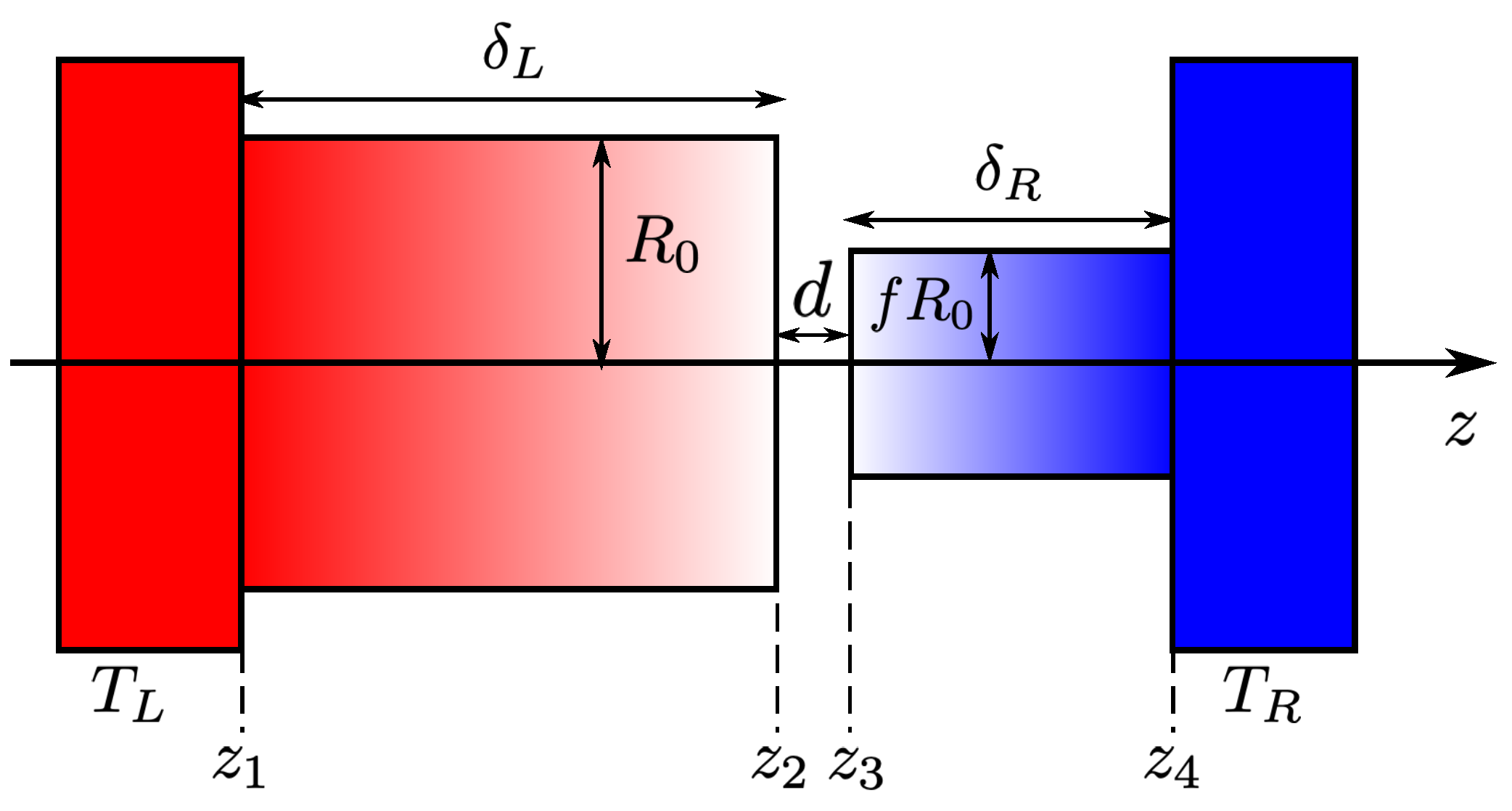
Figure 7.
Two-cylinder scheme employed to simulate the tip–plane configuration. Reproduced from Ref. [43] with the permission of AIP Publishing.
Figure 7.
Two-cylinder scheme employed to simulate the tip–plane configuration. Reproduced from Ref. [43] with the permission of AIP Publishing.

Figure 8.
(a) Radiative heat flux as a function of the distance, d, in a tip–plane configuration (solid lines), slab–slab scenario (dot-dashed lines), and in the absence of coupling (dashed lines). (b) The ratio between fluxes in the presence () and absence () of coupling as a function of the radius, , and the radii fraction, f. The plot corresponds to two SiO cylinders having m at nm. Reproduced from Ref. [43], with the permission of AIP Publishing.

Disclaimer/Publisher’s Note: The statements, opinions and data contained in all publications are solely those of the individual author(s) and contributor(s) and not of MDPI and/or the editor(s). MDPI and/or the editor(s) disclaim responsibility for any injury to people or property resulting from any ideas, methods, instructions or products referred to in the content. |
© 2023 by the authors. Licensee MDPI, Basel, Switzerland. This article is an open access article distributed under the terms and conditions of the Creative Commons Attribution (CC BY) license (https://creativecommons.org/licenses/by/4.0/).
Share and Cite
MDPI and ACS Style
Reina, M.; Gharib Ali Barura, C.; Ben-Abdallah, P.; Messina, R. Conduction–Radiation Coupling between Two Distant Solids Interacting in a Near-Field Regime. Physics 2023, 5, 784-796. https://0-doi-org.brum.beds.ac.uk/10.3390/physics5030049
AMA Style
Reina M, Gharib Ali Barura C, Ben-Abdallah P, Messina R. Conduction–Radiation Coupling between Two Distant Solids Interacting in a Near-Field Regime. Physics. 2023; 5(3):784-796. https://0-doi-org.brum.beds.ac.uk/10.3390/physics5030049
Chicago/Turabian StyleReina, Marta, Chams Gharib Ali Barura, Philippe Ben-Abdallah, and Riccardo Messina. 2023. "Conduction–Radiation Coupling between Two Distant Solids Interacting in a Near-Field Regime" Physics 5, no. 3: 784-796. https://0-doi-org.brum.beds.ac.uk/10.3390/physics5030049