Correction and Validation of Time-Critical Behavioral Measurements over the Internet in the Stage Twin Cohort with More Than 7000 Participants

Abstract

Behavioral data are increasingly collected over the Internet. This is particularly useful when participants’ own computers can be used as they are, without any modification that relies on their technical skills. However, the temporal accuracy in these settings is generally poor, unknown, and varies substantially across different hard- and software components. This makes it dubious to administer time-critical behavioral tests such as implicit association, reaction time, or various forms of temporal judgment/perception and production. Here, we describe the online collection and subsequent data quality control and adjustment of reaction time and time interval production data from 7127 twins sourced from the Swedish Twin Registry. The purposes are to (1) validate the data that are already and will continue to be reported in forthcoming publications (due to their utility, such as the large sample size and the twin design) and to (2) provide examples of how one might engage in post-hoc analyses of such data, and (3) explore how one might control for systematic influences from specific components in the functional chain. These possible influences include the type and version of the operating system, browser, and multimedia plug-in type

1. Introduction

The Internet provides the opportunity to collect information from human participants across infinite distances, wherever there is an on-line computer. Compared to an investigator traveling to where the participants are or participants traveling to a laboratory, web-based data collection tools can reach more people at a lower cost. A large-scale transfer of behavioral data collection to the Internet has consequently taken place over the last decades, and it has become established practice to collect questionnaire and survey data through web interfaces. This is accompanied by an increasing availability of online platforms and software tools that reduce the demands on researchers to design web-interfaces, and to manage the technical intricacies of client-host communication, database management, and multi-platform variability [1,2,3,4,5,6,7,8,9,10,11,12,13,14,15]. “Platform” here refers to the combination of technical alternatives in any given console, including the computer type and performance, its input and output devices, the operating system (OS), and, in the case of web-based measurements, the browser and its plug-in applications, as well as the quality of the Internet connection.

Many types of measurements remain dependent on traveling, for obvious reasons, such as brain imaging and physical performance tests. Between their high level of physical interaction and temporal precision, and the corresponding low levels in a typical questionnaire, there is a range of measurements that could in principle be made with the input and output devices and the versatility of a personal computer connected over the Internet. Examples include memory, cognitive, and perceptual tests, ratings of audio or video material, and implicit association or so-called priming experiments, where participants are exposed to images of such short duration that it is not consciously perceived. Such types of measurements are less often administered over the Internet. One obvious reason is that they are much more specific than is a questionnaire, so there is less chance that a generalized software will suit the particular requirements. Another reason is that the ways in which visual and auditory stimulation varies across platforms may be critical for test performance, whereas this is of no consequence for corresponding in text in a questionnaire. A third reason is that many tests rely on temporal accuracy in stimulus presentation or response measurement, which is known to be poor and to vary across general-purpose computer systems [9,10,11,13,16]. Both temporal delay and variability that vary across platforms decrease reliability and may even obliterate systematic participant effects. Web-based data collection provides much less control than laboratory measurements. It is clear that keyboards, sound cards, mice, and other involved hardware components also vary in the time delays and variances they add to the behavioral measurements [7]. Web-based time-critical tests have nevertheless been used with great success. They have enabled very large-scale cross-national studies, of which the BBC Internet study of sex differences is perhaps the largest to date [17], featuring tests of mental rotation, object location memory, line angle judgement, and category fluency, all of which include some aspect of timing. However, the response times and time limits that these types of tests require are on the order of seconds, while reaction time tests, for example, require a resolution in the range of up to a few tens of milliseconds [18,19]. Here, we share the experience of a very large data collection of time-critical reaction time and time interval production data obtained from 7127 adult twins, sourced from the Swedish Twin Registry. The purpose is twofold.

First, these data have already been reported in about a dozen publications, and will continuously be used in future studies. It is therefore important to validate them through providing a more comprehensive and detailed description of the data processing than is possible in reports focused on their relation to some other variable(s). These data will furthermore, in all likelihood, be used repeatedly for many years to come, because of the large number of participants, that they belong to a twin population, the very wide range of variables, and the fact that they can be linked to any other individual data available in Swedish registers. The Swedish Twin Registry collects data in several waves across their twin participants’ life time, some of which may be linked from other registers and some obtained directly from the twins. This means that novel research questions can be applied to the same individuals, given that the relevant data are already in the database, can be added through new data collections, or can be linked from other registers. For example, current income, number of children, or marital status could be compiled from census data. In the present study, we addressed the so-called STAGE-cohort of Swedish twins born 1959–1985. About one-third agreed to participate in this data collection wave, which was entirely administered online. Data from this wave have been utilized in some two dozen studies [20,21,22,23,24,25,26,27,28,29,30,31,32,33,34,35,36,37,38,39,40,41,42,43].

Second, our efforts to collect also time-critical data online faced us with several problems, some of which were quite unexpected. Although the technical preconditions constantly change, similar problems will occur in future on-line collections of time-critical data. These include differences in time delay or variability between respondents’ computers, which may be related to their hardware and software configurations. They may be attributed to types and versions of the computer, OS, browser, browser multimedia plug-ins, and installed device drivers, as well as interactions between these. The present study provides several examples of such problems, and how they were dealt with. A further complication is confounds between these aspects and demographic categories, such as the level of education. Indeed, it is conceivable that having and using an Apple or PC, laptop or smartphone, iOS or Android, and so forth, varies along the lines of age, sex, occupation, and so on. For example, reaction times increase with age and tend to be longer for women [18,44], and age and sex might therefore be confounded with the effects of platform per se. This phenomenon causes more severe problems than if the variation were merely random, as the demographic categories may, and are even likely to, co-vary with critical variables in the research design. We provide examples of how to deal also with these problems.

The time-critical data analyzed here consist of simple reaction time (SRT) and serial time interval production (ISIP), which have been reported in four studies so far [18,45,46,47]. The analysis is augmented by direct measurements on model platforms, and is segmented by various platform properties obtained from user-strings from each participant’s computer. In addition, we provide results on attrition rates, the frequencies of various platform configurations in the data, and their relation to demographic properties.

2. Method

2.1. Participants

Data were collected from October 2012 to May 2013 from the STAGE cohort of twins born between 1959 and 1985 [48]. This cohort is part of the Swedish Twin Registry (STR), and has been involved in one previous data collection wave that took place in 2005–2006 [48,49]. The full sample that completed the present wave consisted of 11,543 twins—5651 singletons and 5892 that were part of a complete twin pair. The sample comprised 5651 females and 5792 males, with ages between 27 and 54 at the time of responding to the survey (M = 40.7, SD = 7.75). The study was approved by the Regional Ethics Review Board in Stockholm (Dnr 2011/570-31/5, 2011/1425-31, and 2012/1107/32). We approached all twins in the cohort (N = 32,005) by a letter sent to their residence addresses, containing a brief description of the study, and a statement that their participation was voluntary and may be discontinued at any time and that their commencing the web survey would constitute giving informed consent. The letter contained an individual pass code that the participants used to log in to the web survey.

2.2. Instruments: Overview and Instructions

The data collection comprised dozens of instruments (e.g., intelligence tests, personality inventories, clinical evaluation scales) and hundreds of other survey items in total. Many of the latter were customized, concerning, e.g., musical behaviors and experiences, and others were obtained through standardized instruments adapted for the online survey. Here, we have focused on the time-critical tasks, and mention other variables only when they were actually used for the present analyses. Those variables are age, sex, level of education, and intelligence. The two latter are described in Section 2.2.4 below. Age and sex were determined from the STR records.

The time-critical tasks were implemented both as Flash and Shockwave media players, the user interfaces of which were identical. It appeared as a white box in the centre of the browser window, approximately 100 mm tall and 150 mm wide, depending on screen size and resolution. General instructions appeared in black font in the left part of the application window. They were preceded by a Flash application that tested the sound and user input, and managed installation of the media players. In-house experimentation and pilot testing revealed that Shockwave was superior in timing performance, but that it was less commonly installed on users’ computers. Hence, we could not hope to gather even close to all the data with our preferred software, but we still did not want to sacrifice its superior performance by mandating the use of Flash. It was, on the one hand, undesirable to allow this source of variation, but there were substantial advantages in that Shockwave could provide asynchronies (see Section 2.2.3) and more accurate timing, and the consequences were, on the other hand, manageable, as the user strings would tell us which application was used. We therefore settled for a five-tier procedure, which is described in Section 2.5.

The time-critical tasks appeared about 3/4 in the full survey, and were preceded by a test of sound and keyboard functions, as well as of their understanding of the interface. The description and instructions that the participants were given at this point can be found in Appendix A: Instructions for sound and keyboard test. Confirming that all this worked moved them on to the first practice trial. If they instead clicked the button saying that the sound and keyboard did not work properly, they were given the option of running the sound test again (presuming that they made some changes to their set-up).

The stimulus sound files were 250 ms in duration and occupied about 10 kb in wave format, with 22,050 Hz sampling rate. The SRT and ISIP tasks used the same cowbell sound, which had a 2 ms attack before reaching the maximum amplitude, which waned off to about half after 25 ms. The CRT task had sounds of breaking glass and a car horn, both with an attack shorter than 5 ms and a 200 ms sustain. The sound files were pre-buffered when the application started, to avoid delays when reading the sample into the sound card buffer. Timing data were recorded as inter-onset intervals (IOI), computed as the difference between the current master clock time stamp and a previous one, defined by the task at hand. No filtering was applied or needed at the recording stage. In the RT tasks, responses occurring before the stimulus were not registered at all, and missing responses in the ISIP task simply added the preceding duration to the one before the next response.

2.2.1. Simple Reaction Time (SRT) Application

The instructions for this task were: “Your task is to press the space bar as fast as possible after each sound. Use your best/dominant hand. Wait until you hear the sound, and then press the space bar. Click ‘Start’ to begin the test”. When the participant started the first trial there was a silent interval randomly varied from a rectangular distribution from 1.5 to 3.5 seconds before the stimulus was presented through the computer’s speaker or headphones, whichever was connected. The stimulus consisted of a cow-bell sound, whose loudness depended on the equipment and the participant’s settings in the previous set-up stage. A green box with the text “Waiting for your response!” appeared simultaneously with the sound in the middle of the application window, approximately 20 mm tall and 60 mm wide depending on screen size and resolution. This box disappeared when the bar was pressed, which issued the next random interval, and so forth. The application recorded the time interval from the stimulus presentation to the space bar response and stored it in temporary memory until the application ended, when RTs from all blocks of trials were sent to the server. The application was run twice, as detailed in

Table 1. Summary characteristics of the timing tasks.

			Number of Responses		Number of Data Used for Analysis
Task	Block	IOI (ms)	RT/ISMS	ISIP	RT	ISMS/ ASYNC	ISIP
SRT training	1	1500–3500	10		10
SRT	2	1500–3500	25		25
CRT training	3	1500–3500	12		0
CRT	4	1500–3500	25		25
ISMS/ISIP training	5	581	12	20
ISMS/ISIP	6	524	30	35		28 *	33
ISMS/ISIP	7	819	30	35		28 *	33
ISMS/ISIP	8	655	30	35		28 *	33
ISMS/ISIP	9	1024	30	35		28 *	33
ISMS/ISIP	10	655	12	30			28
ISMS/ISIP	11	524	12	30			28
Sum			228	220	60	112	188

Note. * = only for the Shockwave media player.

, the durations of which were about 30 s for the first and 75 s for the second task. The instructions were repeated between blocks.

2.2.2. Choice Reaction Time (CRT) Application

This two-alternative choice reaction time (CRT) was identical to the SRT application, except that it produced one of two sounds, and the task was to press a key on the right side of the keyboard if it was a car horn or a key of the left side if it was the sound of breaking glass. Before the CRT task there was a training block with 12 trials, which also established in the participant the correct association between each hand with each of the two sounds. The data from the CRT task were not used for correction, because they were produced under identical conditions as the SRT data and are therefore redundant for this purpose.

2.2.3. Isochronous Serial Interval Production (ISIP) Application

This application implemented the commonly called “synchronization-continuation task”, which consists of isochronous sensorimotor synchronization (ISMS) to a series of sounds that introduces the pace with which to continue producing intervals (ISIP) when the sounds cease. This task has a long history and has been used to discover many different aspects of timing behavior [50,51,52,53,54,55,56]. The ISMS data will not be considered here because they were, being attained through the same time-critical processes, assumed to have the same timing characteristics as the ISIP data. The instructions were: “Your task is to synchronize to the sounds by tapping the space bar. Use your best/dominant hand. When the sounds cease, continue tapping as before until you hear the word ‘stop’. Click ‘Start’ to begin the test”. The stimulus consisted of a cow-bell sound, whose properties and presentation were the same as for the RT tasks. The application recorded the IOI between each pair of successive taps, and stored them in temporary memory until the application ended, when IOIs from all blocks were sent to the server. The Shockwave version also recorded the so-called asynchronies, that is, the intervals between the stimuli and the taps during the synchronization phase, whereas the Flash version could not do this due to too long computation times that caused the application to lag. The ISIP application was run seven times, with IOIs as shown in Table 1.

2.2.4. WMT Application and Education Level

Intelligence was measured with the Wiener Matrizen Test (WMT) [57], a 24-item matrix reasoning test, which was implemented in Flash and appeared about mid-point in the full survey. A more detailed description of this implementation is found in Mosing and colleagues [27,28,45]. Education was self-reported, the item appearing about 30 items after the WMT. Participants responded by choosing one of the following options from a bullet list, with the question “Which is your highest level of education?”: (1) Primary school (not completed), (2) Primary school (completed), (3) high school (not completed), (4) high school (completed), (5) tertiary education beneath university (not completed), (6) tertiary education beneath university (completed), and (7) university education (not completed), while 8, 9, and 10 denote completed university degree, licentiate, and doctoral degree, respectively.

2.3. Overview of Time-Critical Task Data

Table 1 lists the time-critical tasks in the order that they were administered, and describes their parameters and the number and type of data that they generated. Either the Shockwave or Flash application was used to generate the data, according to the procedure described in Section 2.5.

The whole suite of 11 time-critical tests consisted of two blocks of SRT trials, two blocks of CRT trials, and seven blocks of ISMS/ISIP trials with different inter-onset intervals (IOI). As indicated in Table 1, each participant generated 508 unique time intervals in total, 360 or 248 of which were analyzed. This means that the 7121 participants nominally generated about 3.6 million intervals in total, of which ~751 thousand from the Flash application and ~1.4 million from the Shockwave application were analyzed.

The first of the SRT, CRT, and ISMS/ISIP blocks were for training, and data from the CRT training block were not recorded. The two last of the ISMS/ISIP blocks were for replication of the 524 and 655 ms ISIP. These blocks had few ISMS responses, which were not analyzed for ISMS/ASYNC. The four longer blocks (6–9) thus yielded three types of data: IOIs of taps on the space bar during synchronization (ISMS), during production (ISIP), and asynchronies during synchronization (ASYNC). However, ASYNC data were available only for the Shockwave application. This means that a complete session yielded three reaction time, seven ISIP, four ISMS, and zero or four ASYNC data blocks; that is, 14 or 18 blocks per participant.

2.4. Direct Measurements on Model Platforms

The web-based Flash timing applications were run on eight computers with different configurations to obtain direct measurements of timing delays and variability. The purposes of this were to (1) obtain ballpark values of what variation we could expect from the data collection proper, (2) identify possible errors or weaknesses in our code, as it interacts with different hard- and software configurations, and (3) obtain specific values for certain hard- or software versions that could be used for error correction in the real data. The Shockwave applications were not developed at the time of this testing. The PC computers were all HP Compaq dx2000 with 2.4 GHz clock frequency and 533 MHz bus frequency, and the Apple computer was an iMac 27” (A1312) with 2.66 GHz clock frequency. Testing employed a customized computer keyboard that simulated a space bar press when an electric signal was received through a cable. This cable was connected to the audio output of the tested computer, thus creating a stimulus-response loop. The hardware latency in this loop was negligible (below 100 us). The SRT application was tested by configuring it to collect 400 responses, and once the operator clicked on “start”, the application would produce random foreperiods ending with a sound, which immediately created a response whose latency from the sound was recorded, which also started the next foreperiod, etc. The choice reaction time application was not tested because it used the same time-critical code and was therefore assumed to have the same timing characteristics as the SRT. The ISIP app was tested by configuring it to 1 synchronization response and 400 continuation responses. The operator started an electronic metronome connected to the customized keyboard and then clicked on “start”, and the application then recorded the intervals between each pair of subsequent sounds. The means and SDs of these data are listed in Table 6.

2.5. Procedure

In total, the survey had 343 verbal or rating scale items, the intelligence test with 24 items, the 11 blocks of time-critical trials listed in Table 1, and also four music ability tests for rhythm, melody, and pitch discrimination, as well as absolute pitch naming. The music-related tests are not described here, as they have been reported in detail elsewhere [21,22,28,32,36,41,58,59]. However, only those respondents who played a musical instrument and had been active in sports, and who had done this throughout their childhood, responded to all of these items. There was a considerable amount of branching, such that if one had not received music lessons or been involved in a sport during any of four age ranges (0–5, 6–11, 12–17, and 18 until the present), items relating to those activities during those age periods were skipped. This is why the number of items varies in the following description.

The survey began with an opportunity to install Shockwave, if it was not detected on the computer. Then followed 17–59 items about music experience and possible music training, depending on branching due to responses to earlier items about music experiences, then 20 items related to motivation, 1 to handedness, and 1–9 to sports activities, depending on branching due to a response on involvement in sports activities. Then followed up to 40 items about flow experiences, depending on branching by music and occupational involvement, and 56 items related to personality, which makes a total of up to 185 items. After this came the WMT, followed by 46 items about occupational status and preferences and further personality traits, 20 items about emotional reactions, and 11 items about health. Then followed the timing and musical ability tests, the instructions to which can be found in Appendix A: Instructions for timing and musical ability test.

After this, a Flash application tested the sound reproduction and the key functions of the computer, and branched further to various routes for installing the Shockwave or Flash software, if required. Shockwave was presented first in the web questionnaire, as it was found to have superior temporal accuracy. If the computer did not have Shockwave installed, participants were again given the option to download and install it. Those who declined, or if the installation failed, were branched to the Flash application instead. If Flash was not installed, the participant was given the option to download and install it. Those who declined, or if the installation failed, were branched to the next item in the questionnaire, and continued responding to the next 139 items, comprising 49 about creative activities, 20 about psychological experiences, and 1–12 about work environment, depending on branching due to a response on occupational involvement. After completing the last verbal and rating scale items, a third attempt was made to complete the time-critical tests, and to install a media player if needed.

2.6. Design and Analysis

The following analyses were based on the timing data from the SRT and ISIP tasks and the so-called user strings obtained from the system through the browser, which provides codes that designate, amongst other things, the operating system (OS), browser, and multimedia plug-in type (media player), and version numbers. These system properties can be considered as several independent variables that might affect the timing accuracy and hence the validity of time-critical measurements at the same time, as there may be other variables not covered by the user string, such as computer hardware properties. The number of levels in each of the variables used in the following analyses varied from two, for the type of media player (Flash or Shockwave), three operating systems (OS), up to nine OS versions, and about 50 media player versions. These variables were considered nominal, i.e., we did not expect any particular relationship between levels, such as OS or other software types or versions, and were estimated through mean differences and test that were appropriate, such as t-test or Analysis of Variance (ANOVA).

The analyses of platform effects on timing accuracy were conducted in two main steps. Because we already know about systematic effects of demographic variables such as age and sex, but we do not know if there are any systematic associations between these variables and possible undocumented system properties, it made more sense to correct for these on as broad a level as possible before both investigating, and correcting for, effects on more narrow levels. The results were therefore analyzed for each OS separately in the first step, controlling for age and sex, since these variables entail direct effects on timing not confounded with OS versions. Age is a continuous ratio scale variable, and was therefore analyzed with linear regression. Based on these corrections for individual demographic variables, the data were, in the second step, corrected for the differences in intelligence (WMT) and education level between users of different OSs, in order to enable assessment of possible interactions between all types of method variables. The rationale for this is that the present design had no control over these variables, that is, the equipment that the participants chose for responding to the survey, and any systematic interaction between the system properties and any properties of the participants that may affect their performance thus constitutes an inherent confound. Note that this latter correction is indirect, in that it involves the correction of timing variables on the basis of (1) the relationships between human timing and WMT and human timing and education level, and (2) extant group differences in WMT and education level between operating systems.

3. Results

For the time-critical tests, we computed so-called derived variables for each block of intervals, thus reducing the 10–35 data to 2 data, one central tendency and one dispersion measure. The ISIP and ISMS data were thus described by the mean (M) and standard deviation (SD) and the reaction time data by the median (Md) and the inter-quartile range (IQR). Using non-parametric moments eliminates the influence of possible occasional long delays that typically appear in multi-tasking computer systems [16]. The ISIP/ISMS means were not considered, because they typically reflect the stimulus IOIs accurately, and therefore do not provide information relevant for timing problems incurred by the computer system. For the present purposes, ISIP/ISMS variability was furthermore aggregated across blocks to obtain more stable estimates. Because this variability increases with the IOI, it was standardized to the dimensionless coefficient of variation (CV) × 100 before computing the mean across the six ISIP blocks (6–11). In other words, CV expresses dispersion as a percentage of the mean. Finally, the mean ASYNC was computed as the mean across the four ISMS (6–9) blocks of the mean across the 28 time intervals in each block. Derived variables that reflect dispersion/variability are denoted by a trailing V, and the final list of variables for the following analyses was therefore SRT, SRTV, ISIPV, ISMSV, and ASYNC, that is, four or five data per participant, depending on whether Flash or Shockwave was used.

3.1. Completeness of Data

There were 6916 complete timing files, 3029 of which were made with the Flash application and so lacked asynchrony data, and 3887 made with the Shockwave application. Another 36 data files had minor errors that could be repaired without data loss, such as too many data in some series, which increased the total number of complete timing tests to 6952. There was at least one complete block of trials from a total of 7127 participants, and the missing data were distributed as follows. A total of 8 participants had 9 complete blocks, 15 had 8 complete blocks, 13 had 7 complete blocks, 18 had 6 complete blocks, 9 had 5 complete blocks, 5 had 4 complete blocks, 19 had 3 complete blocks (i.e., only SRT), 68 had 2 complete blocks, and 21 had only the first RT training block. There were thus data from at least one block for 3941 participants collected with the Shockwave and 3186 with the Flash application. This total of 7127 cases was used in following analyses, while their total of 1089 missing blocks of data were ignored. We have no explanation for why some blocks were missing. It is probably because of randomly occurring errors in the chain of operation from the user computer to the downloading of data files from the server. It is also possible that some participant behavior caused the application to proceed without recording any data, although there was no explicit option to skip a survey item.

Some blocks with many outlier values were also excluded. For ISIP 138 blocks of data were excluded because they had more than 50% outliers, according to an automatic outlier elimination procedure. The purpose of this procedure was to exclude clearly non-representative values due to technical triggering problems or failure to perform the task, such as if the participant missed one or a few beats due to fatigue or confusion. Such gross errors would increase the SD dramatically, and it would therefore not make sense to use SD as a criterion. Instead, the outlier elimination procedure replaced values that differed more than 50% from a seven-point running average with the running average excluding the outlier itself. For example, if the nominal value was 524 ms and the running average was 578 ms, a value of 321 ms would be replaced by 578 because 321 + (524/2) = 577, which is less than 578. A too large value would in this case be larger than 578 + (524/2) = 834. Also, SRT blocks were excluded if their median was less than 100 ms (N = 41) or their IQR was greater than 1560 ms (N = 36).

Table 2. Numbers of data points for each of the five derived timing variables.

			RT and RTV *		ISMSV		ISIPV		ASYNC
Task	Block	IOI (ms)	Comp	Out	Comp	Out	Comp	Out	Comp	Out
SRT training	1		7105	16
SRT	2		7108	2
CRT	4		7035	2
ISMS/ISIP training	5	581					6913	105
ISMS/ISIP	6	524			6990	24	6990	27	3935	3
ISMS/ISIP	7	819			6978	27	6976	27	3932	0
ISMS/ISIP	8	655			6964	24	6960	26	3921	0
ISMS/ISIP	9	1024			6953	21	6956	16	3910	2
ISMS/ISIP	10	655					6941	18
ISMS/ISIP	11	524					6928	18
Sum			21,248	20	27,886	96	48,664	237	15,698	5

Note. Comp = complete blocks after possible correction. Out = outlier blocks that were not used. * Either the central measure (M or Md) or dispersion (SD or IQR) was used for all derived variables except RT, from which both were used.

lists how the total 113,496 data points, after 358 such outlier blocks had been excluded, were distributed across the five derived variables. Thus, excluding a whole response sequence with 10-35 data was very rare, constituting less than 0.5% of all blocks. This small number of instances made it impossible to assess if there was any possible systematic relationship between this phenomenon and any platform or participant properties.

3.2. Demographic Analyses

First, we examined whether there were any systematic differences in demographic properties amongst users with different operating systems or platforms. Because reaction times increase with age and tend to be longer for women [18,44], such differences might confound the effects of platform per se if proportions of sex or age differ amongst users of OSs. Windows users (N = 7314, 41.2 yrs) were three years older than Mac OS (N = 1139, 38.3 yrs) and four years older than Linux (N = 52, 37.2 yrs) users. Women were somewhat more likely to use Mac OS than were men (13.7% vs. 13.0%), while the opposite pattern was found for Windows users (84.8% women vs. 86.4% men). The largest platform difference was that Flash yielded about 100 ms longer reaction times than did Shockwave, but there were no systematic age or sex differences in the proportions of users across media players. Simple regressions with age as predictor, the parameters of which are listed in

Table 3. Regression results for age.

Dependent Variable	Intercept	B	β	p	N
SRT	298.72	−0.3535	−0.026	0.0281	6963
SRTV	41.04	0.186	0.030	0.0108	6963
ISIPV	4.97	−0.0036	−0.020	0.092	6963
ASYNC	3.03	0.0057	0.004	0.156	3880

, showed substantial and statistically significant effects for SRT and SRTV. Comparisons of means across the sexes revealed highly statistically significant effects, according to which the women’s values were greater; 2.0 ms longer for SRT (t = 9.46, p < 0.00001), 1.06 for SRTV (t = 13.82, p < 0.00001), and 0.4 for ISIPV (t = 11.89, p < 0.00001). Women were also 7.6 ms earlier in their synchronization (−29.1 ms) than were men (−21.5 ms, t = 4.54, d = 0.15).

Intelligence and education levels were also considered as possible confounds. According to one-way ANOVAs, there were no significant effects of the Windows versions (F_{6, 6083} = 1.69, p = 0.116) or Mac OS versions (F_{17, 929} = 1.47, p = 0.096) listed in

Table 4. Means and standard deviations for each operating system, operating system version, and type of media player (Flash or Shockwave) across participants, corrected for age and sex. Values involving significant differences between OS versions are marked grey.

			ISIPV		ASYNC		SRT		SRTV
Windows Using Flash a	OS ver	N (2345)	M	SD	M	SD	M	SD	M	SD
	XP	383	4.810	1.399			362.08	106.87	53.13	54.57
	Vista	312	4.592	1.378			358.57	129.49	56.45	88.58
	7	1578	4.654	1.515			345.40	111.07	48.15	42.05
	8	54	4.578	1.145			362.47	122.35	44.60	16.15
Windows Using Shockwave b	OS	N (3727)	M	SD	M	SD	M	SD	M	SD
	XP	696	4.649	1.387	−40.54	49.85	232.31	104.05	50.473	90.04
	Vista	639	4.598	1.466	−13.40	52.29	259.46	41.90	41.339	47.33
	7	2326	4.574	1.265	−20.32	49.98	253.40	69.16	44.637	49.23
	8	53	4.470	1.157	−12.18	54.32	256.11	38.98	44.780	32.92
Mac OS Using Flash c	OS ver	N (697)	M	SD	M	SD	M	SD	M	SD
	10.5	15	4.438	0.949			241.05	47.15	39.46	14.12
	10.5.8	24	4.460	1.161			240.62	36.79	46.07	33.03
	10.6	65	4.598	1.509			245.15	38.93	43.00	21.14
	10.6.8	171	4.346	1.156			260.88	84.14	44.33	33.62
	10.7	41	4.189	1.595			247.17	38.40	41.84	23.84
	10.7.4	26	4.104	1.068			280.21	112.27	42.25	18.17
	10.7.5	138	4.289	1.120			267.67	83.48	42.42	18.28
	10.8	28	4.601	2.026			245.24	35.50	50.55	23.83
	10.8.2	157	4.465	1.267			273.36	86.78	49.20	30.38
Mac OS Using Shockwave d	OS ver	N (234)	M	SD	M	SD	M	SD	M	SD
	10.5	9	4.108	1.283	−2.20	71.84	255.54	68.71	41.00	15.65
	10.5.8	14	6.602	2.527	17.45	36.92	268.35	106.56	125.39	311.71
	10.6	21	4.244	1.226	2.76	35.24	241.77	31.31	46.51	22.47
	10.6.8	60	4.287	1.239	−0.96	47.12	250.82	39.06	40.42	17.88
	10.7	12	3.826	1.110	−3.54	68.50	250.86	34.12	38.84	14.53
	10.7.5	43	4.323	1.029	−1.85	46.17	247.14	34.22	43.51	22.56
	10.8.2	51	4.334	1.156	−15.03	48.74	240.89	40.86	49.49	28.37
Linux Using Flash	OS ver	N	M	SD	M	SD	M	SD	M	SD
		44	5.092	1.947			654.63	151.10	56.92	49.44

^a Three cases were omitted with unknown version, 1 case with Windows 2000, and 13 cases with XP 64-bit (5.2). ^b Five cases were omitted with unknown version and eight cases with XP 64-bit (5.2). ^c Five cases were omitted with 10.4, 8 w. 10.4.11, 3 w. 10.6.3, 3 w. 10.6.7, 4 w. 10.7.2, 4 w. 10.7.3, and 3 w. 10.8.1. ^d Two cases were omitted with 10.4, 2 w. 10.4.11, 1 w. 10.6.3, 1 w. 10.6.6, 3 w. 10.6.7, 1 w. 10.7.1, 2 w. 10.7.3, 7 w. 10.7.4, and 8 w. 10.8.

on the level of on education. Information about Linux distributions was not provided by the user string. No significant relationship was found between intelligence and Windows version (F_{6, 6066} = 1.61, p = 0.140) or Mac OS version (F_{17, 926} = 0.63, p = 0.86). However, there were highly significant differences between the three OSs in both WMT (F_{2, 6992} = 18.6, p < 0.0000001) and level of education (F_{2, 6991} = 52.01, p < 0.0000001; all contrasts p < 0.005 according to Tukey’s LSD test, the only exception being between Windows and Linux for education level. Mean WMT scores were 12.92 for Windows (N = 5997), 14.10 for Mac OS (N = 936), and 15.49 for Linux (N = 45). With a grand mean WMT of 12.89 and a SD of 5.31 in the whole sample that took the test correctly (N = 8404), these differences correspond to 3.33 IQ points between Windows and Mac OS, and 4.71 IQ points between Mac OS and Linux. The mean level of education was 6.31 for Windows (N = 5997), 7.18 for Mac OS (N = 935), and 6.62 for Linux (N = 45).

3.3. Controlling for Demographic Variables Procedures

The first step in the analysis, as mentioned in the method section, involved controlling for age and sex, since these variables are known to affect both ISMS/ISIP timing [46] and SRT [18,44]. These corrections were applied to the timing data set used to evaluate and correct for platform differences, not to the final data set used for behavioral analyses, as for them age and sex differences may be relevant. Based on the slopes (B values) in Table 3, the values were corrected with −0.35 ms per year for SRT and −0.18 ms for SRTV, according to highly statistically significant effects. No corrections were made for ISIPV and ASYNC, because the age effects were both small and non-significant. The women’s values were corrected by –2.0 ms for SRT, −1.06 for SRTV, −0.4 for ISIPV, and 7.6 ms for ASYNC, according to the sex differences listed above (only for those using Shockwave).

In the next step, differences between OSs and OS versions were examined on the age and sex-corrected data. For this analysis, the number of levels of one variable differed across the levels of other variables (OS type, OS version, Flash/Shockwave), which made factorial designs unfeasible. We therefore first assessed effects within each condition given by the available combinations of other variables, in this step OS type and OS version. Significant effects were then subjected to specific tests of interactions.

One-way ANOVAs and Tukey’s LSD post-hoc tests were used for testing effects of OS version, separately for each OS. The overall differences between Flash and Shockwave across Windows versions were 4.67 vs. 4.59 for ISIPV (p = 0.028), 350.0 vs. 250.1 ms for SRT (p < 0.000001), and 48.6 vs. 44.0 ms for SRTV (p = 0.00032). Because this is an enormous difference for SRT in particular, analyses in this step were also performed for each OS and timing application type separately. Starting with Windows and Flash, no significant differences were found between OS versions for ISIPV, neither for Flash nor Shockwave application data. There were only two significant differences for RT, in that Vista had 13.2 ms longer SRTs than Windows 7 (W7) (p = 0.0052) and 3.5 ms shorter SRTs than Windows XP (p = 0.0460). The only significant difference for SRTV was that Vista had 8.3 ms higher variability than W7 (p = 0.0072).

For data obtained with the Shockwave application running in Windows, which featured the additional asynchrony measure (ASYNC), there was a substantially larger number of significant differences between OS versions. This is apparently a consequence of the Shockwave application’s smaller variability, which renders mean differences more likely to be statistically significant. XP had significantly shorter SRTs than all other Windows versions. In order of magnitude, XP had 21.1 ms shorter SRT than W7 (p < 0.000001), 23.8 ms shorter than Windows 8 (W8) (p < 0.0223), and 27.1 shorter than Vista (p < 0.000001). The opposite pattern was found for SRTV, in which case XP exhibited 5.8 ms higher variability than W7 (p < 0.0211) and 9.1 ms higher than Vista (p < 0.0044), but no significant difference involving W8. Descriptive data for each combination of media player, OS, and OS version are listed in Table 4.

The overall differences between Flash and Shockwave across Mac OS versions were very small for ISIPV (4.398 and 4.473, respectively, p = 0.45), and moderate for SRT and SRTV. Shockwave yielded 12.6 ms shorter SRTs (248.5 vs. 261.1 ms; p = 0.016), but larger SRTV (54.1 vs. 45.3 ms; p = 0.022). There were 16 versions of the Mac OS amongst the participants that used Flash, ranging from 10.4 to 10.8.2. Table 4 lists the data for versions with more than nine data, thus ignoring versions with so few data that individual differences were likely to play a greater role than OS version (see Table note for excluded OS versions). Tukey’s LSD post-hoc tests showed that RTs were 35.0 ms shorter for version 10.6 than for 10.7.4 (p = 0.048), and 28.2 shorter for version 10.8.2 (p = 0.012), that SRTV was 6.8 ms larger for version 10.8.2 than for 10.7.5 (p = 0.036), and that there were no significant differences for ISIPV.

Mac OS featured 15 versions amongst the participants that used Shockwave, ranging from 10.4 to 10.8.2. The numbers of Shockwave users were substantially smaller in each Mac OS version group, ranging from 1 to 60, as compared to 3 to 171 for those who used Flash. As no significant differences in SRTV, ISIPV, or ASYNC were found amongst OS versions with reasonably large numbers of cases, the corresponding values are not listed in Table 4.

Linux featured five version numbers, a zero for unknown (40 cases) and 12.04 (2 cases), and one each of 9.10, 10.04, and 12.10. This was the only information provided by the user strings, which to our knowledge does not say anything about the Linux distribution. However, the small numbers of cases would have rendered that information useless anyway. Because of the small numbers as well as similar values amongst Flash users, the data were computed across all 44 cases with complete Flash timing data. What we can conclude from this set of analyses is, first, that there are substantial differences between Flash and Shockwave when they run in Windows, but not when they run in Mac OS, and, second, that there are substantial differences between some Windows versions but not between Mac OS versions. It also appears as if the Linux systems used here have very much larger delays and variability, but caution should be taken because of a small number of cases and uncertainty regarding Linux distributions. Taken together, the following analyses should, as a consequence, examine these combinations separately.

The third step of the analysis regarded possible relationships between WMT and level of education on the one hand and the three types of timing variability. As a reasonable compromise based on the previous analyses, these relations were examined for each OS and type of media player separately, to rule out likely spurious effects due to interaction amongst OSs and Flash vs. Shockwave. Linux was not included because of the small number of data. Because of the relationships between WMT and both age and sex [27,46], the regressions used the age and sex-corrected variables. Specifically, linear effects were estimated with multiple regressions with each timing variable as dependent variable and WMT and level of education as predictors. The amount of variance explained by the regression models varied from 0.3 to 3.5 percent, and their parameters are listed

Table A1. Regression results for all four derived variables with WMT and education level as predictors, separately for each combination of OS and media player.

		WMT				Education Level
Windows/Flash
Dependent variable	Intercept	B	β	p	B	β	p	N
SRT	359.14	−1.248	−0.057	0.095	1.081	−0.019	0.37	2265
SRTV	60.24	−0.991	−0.111	<0.00001	0.080	0.004	0.87	2265
ISIPV	5.35	−0.037	−0.130	<0.00001	−0.038	−0.054	0.013	2265
ASYNC
Windows/Shockwave
Dependent variable	Intercept	B	β	p	B	β	p	N
SRT	273.98	−1.274	−0.087	<0.00001	1.024	−0.030	0.076	3624
SRTV	59.10	−1.004	−0.104	<0.00001	−0.290	−0.012	0.48	3624
ISIPV	5.21	−0.036	−0.137	<0.00001	−0.025	−0.039	0.023	3624
ASYNC	−36.01	0.922	0.091	<0.00001	0.198	0.008	0.65	3645
Mac OS/Flash
Dependent variable	Intercept	B	β	P	B	β	p	N
SRT	264.63	−1.169	−0.011	0.78	−0.129	−0.003	0.94	688
SRTV	54.27	−0.795	−0.144	0.0002	0.261	0.016	0.67	688
ISIPV	4.90	−0.047	−0.192	<0.00001	0.018	0.026	0.50	688
ASYNC
Mac OS/Shockwave
	Intercept	B	β	p	B	β	p	N
SRT	271.11	0.995	0.011	0.87	−3.25	−0.112	0.099	231
SRTV	28.75	0.596	0.045	0.60	1.695	0.034	0.62	231
ISIPV	4.83	0.036	0.023	0.06	−0.049	−0.054	0.42	231
ASYNC	−9.04	0.599	0.057	0.39	−0.276	−0.009	0.89	235

(Appendix A). As it turned out that the slopes with WMT as a predictor of ISIPV were quite similar for each OS and media player combination, their mean slope of −0.0389 was used as a correction factor. Likewise, the mean slope for SRT was −1.171 and for SRTV it was −0.846. Finally, the slopes for ASYNC, that were only available for Shockwave data, were 0.92 for Windows and 0.60 for Mac OS. As these numbers were quite different, they were applied as-is.

The slopes with education level as a predictor were considerably smaller and mostly non-significant, indicating that WMT had already accounted for most of the systematic variance, as WMT and education level were themselves substantially correlated (r = 0.289, N = 8084). The slopes for ISIPV in Windows systems were significant, however, so their mean slope of −0.052 was used. Combining these figures with the grand means for WMT (13.09) and level of education (6.43) amongst all participants who completed the timing tests (N = 6996) yielded the correction factors listed in

Table A2. Correction factors for group differences in WMT and level of education for each derived timing variable and OS type, based on the regressions listed in Table A1 and the grand means of the WMT (13.09) and level of education (6.43) amongst all participants who completed the timing tests (N = 6996).

		WMT				Education level
	ISIPV	ASYNC	SRT	SRTV	ISIPV	ASYNC	SRT	SRTV
Windows	0.00661	−0.1564	0.1990	0.1581	0.00428	−0.1012	0.1288	0.1023
Mac OS	−0.03929	0.6060	−1.1827	−0.9393	−0.0291	0.45	−0.8783	−0.6975
Linux	−0.09336	-	−2.8104	−2.232	−0.0121	-	−0.3630	−0.2883

. These are simply the values that were added (or subtracted, in case of negative sign) from all the timing data for each combination of OS type and media player type. Their function is thus to correct for purely participant-specific effects that could be attributable to age, sex, intelligence, and level of education, but not to correct for platform effects. As such, these corrections should increase possible true platform effects by reducing other variability.

3.4. Estimating Platform Effects on Behavioral Data Corrected for Demographic Variables

Thus, having corrected for participant-related variables in the data, we proceeded to analyze differences between browser versions and Flash and Shockwave versions, again for each OS separately. Inasmuch as significant differences were obtained, the strategy was to infer if they can be related to an interaction with OS version, and if so we attempted to correct also for OS version. In cases where no such interactions could be found, the values were accepted as-is. After this, the results were aggregated for each of the derived variables across all versions with non-significant differences, and tabulated together with values for those versions that possibly demonstrated significant differences amongst themselves. Finally, interactions across all these values were sought.

First, as regards numbers, 1111 of Windows users had Explorer, 610 had Firefox, 559 had Chrome, 13 had Opera, and 9 had Safari installed as their browser. Amongst Mac OS users, 471 had Safari, 152 had Firefox, and 72 had Chrome. The OS versions for PC computers running Shockwave were XP (696), Vista (639), W7 (2326), and W8 (53). The OS versions for PC computers running Flash were XP (383), Vista (312), W7 (1578), and W8 (54). Apple computers had Mac OS versions 10.5 to 10.8.2, 234 with Shockwave and 697 with Flash. No significant mean SRT differences were found between Mac OS versions running either Flash or Shockwave, partly owing to small N, in the range 9–171. Again, there were only 44 participants using Linux.

The analyses uncovered several substantial effects of platform components. Windows versions with Flash yielded 50–85 ms longer mean SRTs than both Windows with Shockwave and Mac OS with either Flash or Shockwave. Chrome produced 180–195 ms longer mean SRTs in both Windows and Mac OS than did all other browsers, which affected 631 cases out of the total 7081 that completed the RT tests. In addition, smaller but statistically significant differences were found between Windows versions. Compared to XP, the Shockwave application produced longer mean SRTs in W7 (21 ms), W8 (24 ms), and Vista (27 ms). Compared to W7, the Flash application produced longer mean SRTs in Vista (13 ms) and XP (17 ms). No other mean differences for either Windows or Mac OS were significant.

Table 5. Mean ISIP variability, SRT, and SRT variability for each combination of OS and Browser (data corrected for age, sex, WMT score, and level of education).

	Windows				Mac OS
	N	ISIPV	SRT	SRTV	N	ISIPV	SRT	SRTV
Explorer	1111	4.667	302.43	49.34	0
Firefox	610	4.644	301.92	49.98	152	4.430	243.50	42.64
Chrome	559	4.757	500.54	50.55	72	4.221	425.83	44.53
Safari	9	4.511	305.04	48.35	471	4.315	238.71	43.98
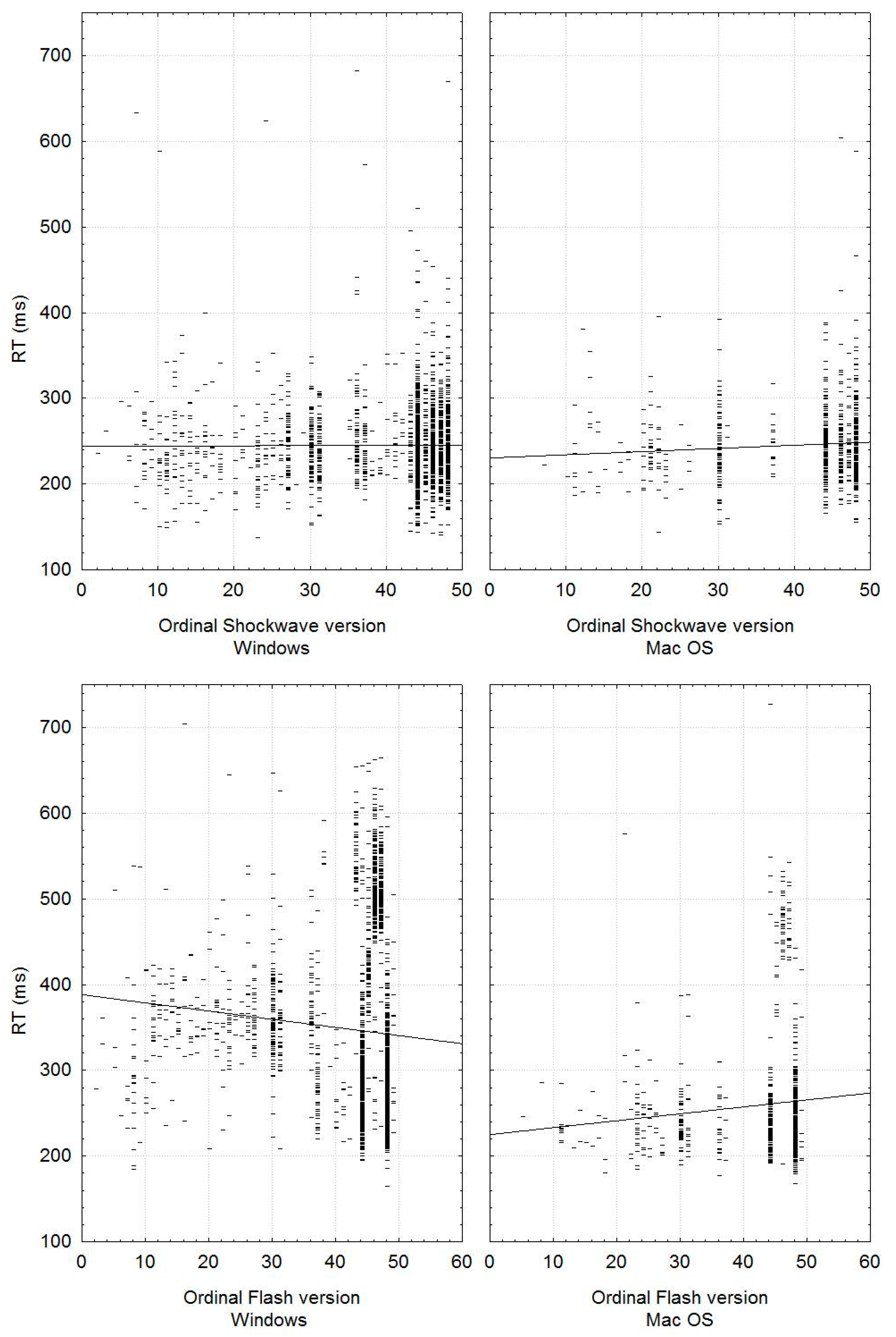
Opera	13	4.490	267.02	50.32	0

lists the means of the derived timing variables as a function of OS (only Windows and Mac OS) and browser, across all other variables. Linux was excluded because it both had few data (44) and very large SRTs (~700 ms). Standard deviations (SD) were excluded to conserve space, but except for SRT they were similar across browsers: for Windows on the order of 1.5% for ISIPV, 69 ms for RT, and 40 ms for SRTV, and for Mac OS 1.5% for ISIPV, 40 ms for SRT, and 25 ms for SRTV. The much larger SDs for Windows indicate larger platform differences, and extensive cross-tabulations showed that its source is Flash versions as well as Flash versus Shockwave, as mentioned before. Across Flash and Shockwave versions, however, Chrome stood out as yielding approximately 200 ms longer SRTs than the other browsers (p < 0.01, according to LSD). LSD tests of the 45 Flash versions were conducted for each OS and browser separately (see

Table A3. Coding of Flash versions into the ordinal numbers used in the present analyses, together with the number of occurrence of each version, and for which browser and OS (1-3) they occurred.

Ordinal Flash Version	N	Version	Explorer	Firefox	Chrome	Safari	Opera
3	2	9.0.280	1
4	2	9.0.470	1			2
5	4	9.0.1545	1			2
6	2	10.0.1236	1	1
7	12	10.0.2287	1	1
8	32	10.0.3218	1	1,2
9	5	10.0.4234	1	1
10	13	10.0.452	1	1
11	43	10.1.10xxx	1	1,2		2
12	17	10.1.536x	1	1		2
13	11	10.1.8276	1	2
14	20	10.1.853	1	2,3		2
15	13	10.2.15226	1	1		2
16	20	10.2.1523x	1	1,2	1	2
17	18	10.2.1531	1	1,2		2
18	20	10.2.1591	1	1,3		2
19	7	10.2.16xxx	1	3
20	13	10.3.18114	1	1
21	24	10.3.1812x	1	1,2		2
22	24	10.3.18134	1	1,2,3	1	2
23	66	10.3.1831x	1	1,2		1,2
24	20	10.3.1832x	1	1,2	2	2
25	23	10.3.18xxx	1	1,2		2
26	32	10.3.1837	1	1,2		2
27	52	11.0.1152	1	1,2,3		2
29	2	11.0.198	1	3
30	197	11.1.10255	1	1,2	2	1,2	3
31	88	11.1.10263	1	1,2		2
32	1	11.1.11110				2
33	1	11.1.11512				2
35	2	11.2.202147	1
36	146	11.2.2022xx	1	1,2,3	1,2,3	2	3
37	78	11.3.3002xx	1	1,2	1	2
38	8	11.3.312xx	1		1,3
39	1	11.3.37294	1
40	13	11.3.37612	1
41	10	11.3.37715	1
42	6	11.3.3785	1
43	61	11.4.31110			1,3
44	872	11.4.4022xx	1	1,2	2	1,2	1
45	146	11.5.31137			1,2
46	378	11.5.312			1,2,3
47	296	11.5.315			1,2,3
48	1667	11.5.5021xx	1	1,2	1	1,2	1
49	34	11.6.6021xx	1	1,2	1,2	2

Note. Numbers in browser columns designate operating system: 1 = Windows, 2 = Mac OS, or 3 = Linux. Version numbers may be aggregates of lower order versions, whose lower order numbers are then replaced with x.

in the Appendix A for the version numbers). For Chrome and both Windows and Mac OS, ISIPV was larger for the version indexed 49 and SRT was larger for those indexed 45–47 (most differences amongst versions indexed 2–49 were also significant, p < 0.05). There were no differences for SRTV when versions used by less than 10 participants were excluded. For comparison, the same tests were conducted for Chrome and the 18 Shockwave versions (see

Table A4. Coding of Shockwave versions into the ordinal numbers used in the present analyses, together with the number of occurrences of each version, and for which browser and OS (1-3) they occurred.

Ordinal Shockwave Version	N	Version	Explorer	Firefox	Chrome	Safari	Opera
2	44	10	1	1,2	1	2	1
3	92	11.5	1	1,2	1	2
4	66	11.6	1	1	1	2	1
5	19	12.0	1		1	2
6	31	11.03	1	1	1	2
7	110	11.51	1	1	1	2
8	43	11.52	1	1	1	2
9	79	11.56	1	1,2	1,2	2	1
10	114	11.57	1	1	1
11	77	11.58	1	1	1
12	291	11.59	1	1,2	1	2	1
13	161	11.61	1	1	1,2	2	1
14	151	11.63	1	1	1	2
15	133	11.64	1	1,2	1,2	1,2
16	148	11.65	1	1,3	1,2	2	1
17	110	11.66	1	1,2	1,2	2
18	91	11.67	1	1	1
19	2241	11.68	1	1,2	1,2	1,2

Note. Numbers in browser columns designate operating system: 1 = Windows, 2 = Mac OS, or 3 = Linux.

in the Appendix A for the version numbers). Whether run in Windows or Mac OS, no differences were found for any variable with more than 10 data, which was also true when all browsers running under Mac OS were considered. For Windows, however, this was true only for SRTV, whereas there were several significant contrasts amongst the Shockwave versions for ISIPV, SRT, and ASYNC. It could clearly be seen that Flash versions 11.5.311–11.315 yielded qualitatively different data with higher mean SRT and variability, indexed 45–47 in Figure 1. However, Table A3 also shows that these version numbers coincided with Chrome, an example of the complexity of these independent variables.

We conclude that the patterns of platform effects are very complex. They contain both strong confounds in the sense that some Flash and Shockwave versions only occurred together with some OSs, OS versions, browsers, and browser versions, and difficult evaluations of difference values in combination with their significance levels and N. What we can safely say is that the presence of relatively large systematic individual differences, although corrected for some demographic variables, make it inappropriate to correct for means based on small N. Significant effects occurred repeatedly even for very small N, which may either be a true platform effect or the result of particularly large individual differences, a random artefact, or a confound between a platform effect and some unmeasured individual variable. There is therefore a risk that the correction of relatively small groups introduces more noise, as it might by chance eliminate a fraction of the true differences between individuals.

3.5. Direct Measurements

We also attempted to directly measure system delays and variances. The first result we can note from

Table 6. Timing delays and variability for eight computer systems.

	SRT app		ISIP app
	M	SD	M	SD
Windows XP, Internet Explorer	18.84	2.71	498.67	24.3
Windows XP, Firefox 12.0	23.65	5.96	500.27	9.10
Windows XP, Chrome	22.53	2.89	500.25	4.56
Windows 7, Chrome	85.94	5.73	499.98	10.85
Windows 7, Firefox 12.0	87.80	7.41	500.63	6.61
Windows 7, Internet Explorer	64.43	4.04	500.06	4.04
Windows 7, Chrome 20.0.1132.47	87.72	5.27
Mac OS X 10.7.4, Safari 6.0	53.77	4.36	503.24	6.23

Note. Each value is based on 400 responses. ISIP variability is given in ms, but in the results section in Coefficient of Variation (CV) x 100, in other words dispersion as a percentage of the mean. For the first row for example, the SD of corresponds to a CV of 4.86 (24.3/499 × 100 = 4.86).

is that all configurations were very accurate in measuring the mean IOIs, whose means across 400 intervals were all within ±1.3 ms. Differences in delays and variability were substantial, however. W7 entailed almost three times as long delays as did XP, with Mac OS halfway in between. Likewise did the Firefox browser entail twice as large variability than did Chrome and Internet Explorer, but this difference was smaller in W7 than in XP.

It is an important result that the timing variability is so large and differs as much across different software (as the hardware was the same for the Windows platforms). The magnitude of both delays, variabilities, and their differences across platforms are many orders of magnitude larger than what might be expected from hardware properties, such as clock frequency. Even the first personal computer, the IBM XT, with a clock frequency of 4.77 MHz, would entail a temporal variability of less than 1 ms, assuming around 50 basic processor operations per measurement cycle. It is apparently not the hardware that constitutes the bottleneck for precise timing, but the way that the software is designed for multi-purpose computers, including the operating systems themselves [16]. This points to the importance of tracking the software versions in users’ computer when conducting time-critical online measurements.

There were however several problems. First, the direct measurements did not include the Shockwave applications, as explained in Section 2.4. Second, the direct measurements provided no user strings, and version numbers was therefore read off from the applications themselves. That this information was obtained in a different format than the behavioral tests created confusion as to its comparability. Third, some platform configurations were not even found in both the benchmark and behavioral data, and could thus not be applied. Fourth, any way we attempted to relate the patterns across the eight model systems listed in Table 6 with the behavioral data provided poor correspondence. For example, the 87.8 ms delay and 6.61 ms variability for a Windows 7 system with Firefox would indicate that these values could be subtracted from the behavioral values, but in fact, this would in numerous cases yield negative values, which is of course unreasonable. In concert, these discrepancies suggest that there are additional factors that affect the timing inaccuracy, be they either random or unmeasured. If they are unmeasured, they may in fact to some extent be detected by the post-hoc analysis of the behavioral data. Considering all these concerns, we decided to ignore the direct measurements in the correction with the argument that we can only be sure that the behavioral data actually contains the specific system error that we want to control for.

3.6. Correcting for Platform Effects Based on Behavioral Data Corrected for Demographic Variables

Based on the present results and conclusions, the best approach for correction seems to be piecewise independent N-weighted correction. This means that correction values are calculated independently for each platform variable and then aggregated for each case. Specifically, the value for each level of the current platform variable will be subtracted from the mean across all levels, which yields a positive value when that value is smaller than the mean and vice versa. This is only done for variables that are in fact independent. Obviously, OS version was only relevant with respect to a particular OS, browser version only to a particular browser, Flash version only to Flash, and Shockwave versions only to Shockwave, which means that there were four levels of correction values. The series of these four values was added to each raw value for each case. To account for N and the risk that values based on small N are incorrect one could set a cut-off such that the correction values for platform variable levels with small N are set to 0. However, as just mentioned, the appropriateness of correcting depends both on N and the platform effect, which is not directly known. Although it is in principle computable, the sheer amount of effects to consider would be enormous. A more straightforward method is to weight the differences by their proportional N according to W(X) = N(X)/N_total.

3.7. Implementation of Corrections for Platform Timing Differences

As reported above, the corrections occurred as vectors of N-weighted discrete values related to each level in several method variables for each variable specifically (e.g., browsers, media player versions). Because of the complexity entailed by different numbers of levels between methods, and interactions between methods, the corrections were implemented as iterative subtractions from the raw values, rather than attempting to produce joint mathematical expressions. Concretely, the corrections were made with a visual basic script in Statistica 7.1, which subtracted values from a table according to a conditional loop for each case in the data matrix. To give an impression of the effects of the corrections,

Table 7. Comparison of means and standard deviations of raw and corrected SRT, CRT, and ISIPV for each year cohort.

	SRT Raw		SRT Corrected		CRT Raw		CRT Corrected		ISIPV Raw		ISIPV Corrected
Age	M	SD	M	SD	M	SD	M	SD	M	SD	M	SD
27 *	295.8	84.9	248.7	35.8	485.0	116.9	442.2	84.9	4.759	1.138	4.688	1.143
28	295.1	99.1	250.4	51.4	503.1	170.9	465.7	150.8	4.821	1.494	4.731	1.501
29	293.6	93.4	247.3	53.8	501.8	144.9	461.7	119.9	4.936	1.468	4.852	1.456
30	303.9	104.1	249.7	62.8	525.5	149.8	480.7	123.8	4.788	1.243	4.700	1.242
31	291.3	104.6	245.0	68.2	517.7	194.0	477.1	177.7	4.974	1.579	4.889	1.589
32	288.3	89.1	242.8	51.2	509.7	127.8	471.2	105.0	4.926	1.429	4.833	1.427
33	282.2	91.2	243.0	58.2	492.5	146.8	461.2	134.6	4.752	1.366	4.661	1.359
34	286.1	91.9	241.3	47.6	516.2	155.6	480.7	145.2	4.863	1.918	4.773	1.919
35	276.8	83.5	238.8	46.1	498.3	110.1	465.6	91.8	4.884	1.179	4.773	1.181
36	274.3	91.4	238.3	52.3	495.1	144.4	463.0	125.9	4.805	1.318	4.696	1.325
37	278.9	90.5	241.0	55.6	499.0	127.4	467.2	110.7	4.814	1.355	4.705	1.361
38	279.8	94.9	239.0	49.1	510.8	143.9	479.6	126.0	4.973	1.433	4.842	1.426
39	275.0	81.5	243.1	49.5	500.6	144.8	472.5	132.7	4.872	1.356	4.764	1.338
40	272.0	90.4	237.6	54.4	506.4	179.2	477.8	164.3	4.868	1.443	4.751	1.453
41	266.9	80.1	235.3	42.7	497.9	121.7	473.1	110.0	4.650	1.238	4.524	1.237
42	287.8	103.2	238.9	66.2	520.3	139.0	484.8	121.6	4.990	1.324	4.879	1.331
43	276.0	82.7	241.1	45.4	511.1	152.0	481.1	140.6	4.831	1.296	4.724	1.312
44	274.9	90.7	241.8	60.2	528.5	233.3	499.2	223.1	4.726	1.091	4.595	1.085
45	266.8	75.3	238.6	49.6	503.0	126.1	477.2	108.3	4.748	1.453	4.627	1.465
46	272.6	82.1	242.8	48.2	510.7	137.8	484.4	124.3	4.620	1.372	4.483	1.355
47	278.3	86.7	246.3	62.6	530.7	156.5	502.5	147.8	4.903	1.497	4.795	1.489
48	273.9	82.0	242.2	56.4	520.1	125.6	491.7	113.3	4.874	1.355	4.756	1.362
49	280.3	84.6	240.0	48.8	526.5	128.5	490.0	103.2	4.712	1.374	4.596	1.382
50	284.7	80.2	249.4	54.0	531.4	162.9	500.1	153.4	4.725	1.421	4.616	1.414
51	291.9	99.5	250.6	62.2	544.4	165.4	506.7	145.2	4.781	1.315	4.656	1.320
52	291.3	99.5	251.3	61.8	547.2	177.0	510.1	156.4	4.840	1.360	4.744	1.376
53	281.4	84.7	251.8	63.2	548.8	239.1	522.5	234.8	4.832	1.333	4.713	1.315
54 *	302.0	110.0	254.5	89.8	557.1	128.5	510.8	115.1	4.984	1.255	4.871	1.259
M across age	282.2	90.6	243.7	55.5	515.8	157.2	482.9	142.2	4.826	1.393	4.718	1.394

N = 7081 for SRT (201–310 * per age group); N = 7033 for CRT (200–306 * per age group); N = 6985 for ISIPV (200–307 * per age group). * excluding 27 and 54 years, for which there were substantially fewer participants, i.e., 64–97.

shows means and SDs for SRT, CRT, and ISIPV before and after correction. These statistics are categorized by participant age in Table 7, in order to assess the consistency across some partitioning of the data, and because there were significant differences across birth years [18].

The differences between raw and corrected values in Table 7 are consistent with the results in general. The largest differences were obtained for SRT, reflected in very much larger variability for the raw values. There was also a tendency that particularly large SDs, as for 30, 31, and 42 years of age, became more similar to other age cohorts after correction. It is likely that these cohorts had by chance a more even proportion of Chrome vs. other browsers (see Figure 1 and Table A3 and Table A4), or some other major difference between method variables. For CRT, the differences between raw and corrected values were smaller but consistently in the direction of lower SDs. This shows that the correction has decreased variability across individuals, which means it has either decreased variability due to platform effects or to individual differences per se. Finally, the SD of ISIPV did not decrease at all, consistent with the fact that these differences between platforms were very small and in no case statistically significant. It is therefore questionable if the ISIPV correction increased the validity of the measurements. To assess this issue, a final analysis considered correlations amongst the three timing measures as well as with a validation variable, for raw and corrected values separately. The most relevant validation variable present in this dataset was the WMT score, which is also included in

Table 8. Correlations amongst raw timing values, corrected timing values, and between both raw and corrected timing values and WMT (intelligence) as a validation variable (N = 4902).

	Raw Values			Corrected Values
	SRT	CRT	ISIPV	SRT	CRT	ISIPV
CRT	0.585			0.400
ISIPV	0.086	0.137		0.119	0.130
WMT	−0.074	−0.106	−0.163	−0.158	−0.119	−0.163

. Only participants who completed both the WMT and the timing tests were included (N = 6973), and only one member of each complete twin pair was also excluded (N = 2071) so as not to create spurious correlations because of their high behavioral similarity.

The results in Table 8 are consistent with the presence of platform effects, inasmuch as correlations between timing measures related to the same (SRT and CRT) aspect (delays) decrease after correction, but those related to different aspects (delays and variability) increase (SRT and ISIPV). This was, however, not true for CRT. It is also consistent with decreased error variability, as correlations with the validation variable (WMT) tended to increase. The correlation between WMT and ISIPV did not change, however, which probably has to do with these corrections being very small.

4. Discussion

The purposes of the present study were to provide a comprehensive and detailed description of how these timing data were processed and corrected for platform effects, as they have and will be used in many studies, and to provide concrete examples of these kinds of platform effects, and how they can be dealt with. Taken together, the results indicate that web-based collection of these variables entails considerable loss in reliability, even after correction. For example, SRT has been used in Mosing, Verweij, Madison, Pedersen, Zietsch, and Ullén [28], Madison, Mosing, Verweij, Pedersen, and Ullén [47], and Madison, Woodley of Menie, and Sänger [18], and ISIP in Mosing, Verweij, Madison, and Ullén [46] and Ullén, Mosing, and Madison [45]. Correlations have been about −0.17 between both SRT and ISIP and intelligence, but around 0.3 between intelligence and related indices that are not time-critical, such as WMT and rhythm discrimination [46]. Likewise, WMT was stronger correlated (~0.35) with musical ability test performance than with SRT (−0.10), although SRT and ISIP measured in laboratory settings are typically correlated with intelligence at 0.3–0.5 [60,61,62]. The major effects of the correction were rather to decrease inflated RTs due to system delay, and decrease the mean inter-individual variability. In accordance with the figures in Table 7, this was found to decrease SD within each age cohort from 90.6 to 47.9 ms, although it made only a marginal difference to the main result in a study on secular change in SRT [18].

The present study could not determine to which extent this lower reliability is due to temporal inaccuracy inherent in the instruments, or to differences in behavior related to the situation. This is because the data were collected online, which considerably decreases the researchers’ control over the participants. Madison et al. [18] discussed several sources of behavior-related reliability threats. ISIP and reaction time tasks are repetitive and tend to be perceived as boring, which may be one reason why they might have been affected by the situation more than other tests performed under the same conditions [21,22,27,29,59]. The threshold for fluking the task may also be much lower when participants (1) work for free, (2) perform the tests in the comfort of their own homes, and (3) feel less obligation to anonymous researchers that they have not met, or even know the names of. It can also be argued that they require more focus and determination to be performed close to the individual’s top level of performance, compared to the WMT and musical ability tests [59].

The direct measurements of timing inaccuracy, without participants involved, should in principle yield the best benchmark data for method correction. As it turned out, we could not use those data to control for the data proper, because they were incongruent with the differences in the behavioral data across comparable platforms. We had admittedly only one Mac OS system, and did not cover all possible combinations of current types and versions of OSs, browsers, and media players. However, already this combinatorial space soon becomes unmanageable, both in terms of setting up and administering all these direct tests and analyzing and interpreting the results. This disappointing lack of coherence may also to some extent be attributed to additional sources of variation that are more difficult or impossible to control for, such as hardware (processors, clock frequencies, hard drive and bus data transfer speed, sound cards, keyboards, etc.) and software (other programs that use system resources, drivers), and Internet-related things like bandwidth and more or less temporary communication failures. Furthermore, we did not know beforehand which of all the known method variables would be most important so that we could include design features that focus on them.

That SRT and CRT means became lower after correction is trivial, but it is notable that they became more similar to auditory SRT and CRT found for comparable participants in studies with the shortest RTs, which indicates that they used equipment with minimal delays. Considering only studies with more than 50 participants from the general, typically functioning population, median or mean SRTs have been reported at 209 ms [63], 240–259 ms [64], and 220–280 ms for young to middle-aged adults [65,66]. There are, however, also studies that have indicated both substantially shorter and longer auditory reaction times. The former studies are typically older, and the explanation could be that before computers were readily available, researchers used equipment with almost no delay at all, either mechanic (e.g., [67], 120–200 ms) or electronic hardware ([66], 175–220 ms), [68]. Another explanation could be that reaction times have increased across generations [18,19,44,69]. Consistent with the first explanation is that studies reporting longer RTs used various forms of computerized testing. It is notable that none of them reported the inherent delay and variability of their measurement setup. In such studies are mean simple auditory RTs reported as, for example, 284 ms [70] and 415 ms [71]. These large differences across studies highlight the influence of different methods. Dodonova and Dodonov [72] listed a range of factors that may differ across reaction time studies, and that entail RT differences on the order of 10–30 ms, but did not acknowledge that errors related to general purpose computer systems can be considerably larger [16], and thus typically overshadow the former. It is therefore disconcerting that the delays and variability in instruments for measuring time-critical behavior are seldom reported [73,74,75].

The participants in this study were a unique sample of twins, and it was a priority to recruit as many as possible. We therefore sacrificed accuracy for inclusiveness, as we considered but rejected several optional scenarios in which we required certain software versions or distributed a package of software that each participant had to install on her computer, in order to standardize the platform to some extent. Even regarding such an important component as the media player, we allowed each participant to use Flash if she did not have or would not download Shockwave, not to risk greater attrition.

A less unique and exclusive population of participants would allow for considerably greater control. If participants are paid and exchangeable, it would be feasible to demand customization of their home computer by, for example, installing certain browsers, media players, etc. This also opens the possibility to go yet one step further and require installing customized software, which makes it possible to by-pass both media players and browsers, and thereby eliminate related variability. In concert, one could require participants to turn off or uninstall software known to create time lags, such as Groove (© Microsoft Corporation) or Outlook (© Microsoft Corporation), which demands considerable resources when polling the email servers. In principle, one could even require a certain OS, of which Windows XP would have been strongly preferred at the time of this data collection [16], see also Table 4 and Table 6.

In conclusion, computerized time-critical testing is subject to considerable delay and variability, the largest part emanating from the software, but much of this can be controlled through a range of different measures. The present study as well as the reviewed literature show that negligible or constant measurement variation cannot be assumed under any circumstances, and that it is therefore essential to assess this variation under all conditions. Only when the variation is known can its influence on the results and their validity and reliability be assessed, and possible remedies be conceived.

The present study provides some guidance for conducting similar studies. It stands to reason that media players are quite different, as they are the engine that runs the time-critical processes. What was somewhat surprising, however, was that their performance was overall so poor that their relative differences played a large and perhaps even the largest role for the platform effects. Future studies should therefore stick to one type, unless one collects so much data that reliable comparisons and corrections can be made, as in the present study. Another somewhat surprising result was the substantial differences between some versions of the same software (browsers and media players). This speaks for demanding or at least strongly encouraging users to update all relevant software to the current versions before conducting time-critical tests online. This issue might perhaps be circumvented altogether by other technical solutions that, for example, facilitate running the tests directly on a server (see, e.g., [5,11]). This is outside the scope of the present paper, but it should be cautioned that this might merely move the delays and timing variability from the local system to the Internet transmission of time-critical stimulus and response events [14].

References

- Barnhoorn, J.S.; Haasnoot, E.; Bocanegra, B.R.; Van Steenbergen, H. QRTEngine: An easy solution for running online reaction time experiments using qualtrics. Behav. Res. Methods 2014, 47, 918–929. [Google Scholar] [CrossRef] [Green Version]
- Garaizar, P.; Vadillo, M.A.; López-De-Ipiña, D. Presentation accuracy of the web revisited: Animation methods in the HTML5 Era. PLoS ONE 2014, 9, e109812. [Google Scholar] [CrossRef] [PubMed]
- Garaizar, P.; Vadillo, M.A. Accuracy and precision of visual stimulus timing in PsychoPy: No timing errors in standard usage. PLoS ONE 2014, 9, e112033. [Google Scholar] [CrossRef] [PubMed]
- Garaizar, P.; Vadillo, M.A.; López-De-Ipiña, D.; Matute, H. Measuring software timing errors in the presentation of visual stimuli in cognitive neuroscience experiments. PLoS ONE 2014, 9, e85108. [Google Scholar] [CrossRef] [PubMed]
- Stoet, G. PsyToolkit: A novel web-based method for running online questionnaires and reaction time experiments. Teach. Psychol. 2017, 44, 24–31. [Google Scholar] [CrossRef]
- Slote, J.; Strand, J.F. Conducting spoken word recognition research online: Validation and a new timing method. Behav. Res. Methods 2015, 48, 553–566. [Google Scholar] [CrossRef] [Green Version]
- Woods, A.; Velasco, C.; Levitan, C.A.; Wan, X.; Spence, C. Conducting perception research over the internet: A tutorial review. PeerJ 2015, 3, e1058. [Google Scholar] [CrossRef] [Green Version]
- Reimers, S.; Stewart, N. Presentation and response timing accuracy in Adobe Flash and HTML5/JavaScript Web experiments. Behav. Res. Methods 2015, 47, 309–327. [Google Scholar] [CrossRef]
- Schreiner, M.; Reiss, S.; Schweizer, K. Method effects on assessing equivalence of online and offline administration of a cognitive measure: The exchange test. Int. J. Internet Sci. 2014, 9, 52–63. [Google Scholar]
- Schubert, T.W.; Murteira, C.; Collins, E.; Lopes, D. ScriptingRT: A software library for collecting response latencies in online studies of cognition. PLoS ONE 2013, 8, e67769. [Google Scholar] [CrossRef] [Green Version]
- De Leeuw, J.; Motz, B. Psychophysics in a web browser? Comparing response times collected with JavaScript and Psychophysics Toolbox in a visual search task. Behav. Res. Methods 2015, 48, 1–12. [Google Scholar] [CrossRef] [PubMed] [Green Version]
- Hilbig, B.E. Reaction time effects in lab-versus web-based research: Experimental evidence. Behav. Res. Methods 2015, 48, 1718–1724. [Google Scholar] [CrossRef] [PubMed]
- Pinet, S.; Zielinski, C.; Mathot, S.; Dufau, S.; Alario, F.-X.; Longcamp, M. Measuring sequences of keystrokes with jsPsych: Reliability of response times and interkeystroke intervals. Behav. Res. Methods 2016, 49, 1163–1176. [Google Scholar] [CrossRef] [PubMed] [Green Version]
- Plant, R.R. A reminder on millisecond timing accuracy and potential replication failure in computer-based psychology experiments: An open letter. Behav. Res. Methods 2015, 48, 408–411. [Google Scholar] [CrossRef] [PubMed] [Green Version]
- Chetverikov, A.; Upravitelev, P. Online versus offline: The web as a medium for response time data collection. Behav. Res. Methods 2015, 48, 1086–1099. [Google Scholar] [CrossRef] [Green Version]
- Wallace, A. The timing accuracy of general purpose computers for experimentation and measurements in psychology and the life sciences. Open Psychol. J. 2012, 5, 44–53. [Google Scholar] [CrossRef]
- Reimers, S. The BBC internet study: General methodology. Arch. Sex. Behav. 2007, 36, 147–161. [Google Scholar] [CrossRef]
- Madison, G.; Woodley of Menie, M.A.; Sänger, J. Secular slowing of auditory simple reaction time in Sweden (1959–1985). Front. Hum. Neurosci. 2016, 10, 407. [Google Scholar] [CrossRef] [Green Version]
- Woodley, M.A.; Nijenhuis, J.T.; Murphy, R. Is there a dysgenic secular trend towards slowing simple reaction time? Responding to a quartet of critical commentaries. Intelligence 2014, 46, 131–147. [Google Scholar] [CrossRef]
- Turner, J.R.; Arkes, H.R. Piagetian stage and preferred level of complexity. Psychol. Rep. 1975, 37, 1035–1040. [Google Scholar] [CrossRef]
- Mosing, M.A.; Madison, G.; Pedersen, N.L.; Kuja-Halkola, R.; Ullén, F. Practice does not make perfect. Psychol. Sci. 2014, 25, 1795–1803. [Google Scholar] [CrossRef] [PubMed] [Green Version]
- Mosing, M.A.; Pedersen, N.L.; Madison, G.; Ullén, F. Genetic pleiotropy explains associations between musical auditory discrimination and intelligence. PLoS ONE 2014, 9, e113874. [Google Scholar] [CrossRef] [PubMed]
- Theorell, T.; Lennartsson, A.-K.; Mosing, M.A.; Ullén, F. Musical activity and emotional competence—A twin study. Front. Psychol. 2014, 5, 774. [Google Scholar] [CrossRef] [PubMed] [Green Version]
- Menie, M.A.W.O.; Figueredo, A.J.; De Baca, T.C.; Fernandes, H.B.F.; Madison, G.; Wolf, P.S.A.; Black, C.J. Strategic differentiation and integration of genomic-level heritabilities facilitate individual differences in preparedness and plasticity of human life history. Front. Psychol. 2015, 6, 422. [Google Scholar]
- Menie, M.A.W.O.; Madison, G. The association between G and K in a sample of 4246 Swedish twins: A behavior genetic analysis. Pers. Individ. Differ. 2015, 74, 270–274. [Google Scholar] [CrossRef]
- Theorell, T.; Lennartsson, A.-K.; Madison, G.; Mosing, M.A.; Ullen, F. Predictors of continued playing or singing—From childhood and adolescence to adult years. Acta Paediatr. 2015, 104, 274–284. [Google Scholar] [CrossRef] [PubMed]
- Mosing, M.A.; Madison, G.; Pedersen, N.L.; Ullén, F. Investigating cognitive transfer within the framework of music practice: Genetic pleiotropy rather than causality. Dev. Sci. 2015, 19, 504–512. [Google Scholar] [CrossRef]
- Mosing, M.A.; Verweij, K.J.H.; Madison, G.; Pedersen, N.L.; Zietsch, B.P.; Ullén, F. Did sexual selection shape human music? Testing predictions from the sexual selection hypothesis of music evolution using a large genetically informative sample of over 10,000 twins. Evol. Hum. Behav. 2015, 36, 359–366. [Google Scholar] [CrossRef]
- Ullén, F.; Harmat, L.; Theorell, T.; Madison, G. Flow and individual differences—A phenotypic analysis of data from more than 10,000 twin individuals. In Flow Experience: Empirical Research and Applications; Harmat, L., Orsted Andersen, F., Ullén, J., Wright, J., Sadlo, G., Eds.; Springer: Heidelberg, Germany, 2015; pp. 1–26. [Google Scholar]
- Verweij, K.J.H.; Mosing, M.A.; Ullén, F.; Madison, G. Individual differences in personality masculinity-Femininity: Examining the effects of Genes, environment, and prenatal hormone transfer. Twin Res. Hum. Genet. 2016, 19, 87–96. [Google Scholar] [CrossRef] [Green Version]
- Menie, M.A.W.O.; De Baca, T.C.; Fernandes, H.B.F.; Madison, G.; Figueredo, A.-J.; Aguirre, M.P. Slow and steady wins the race: K positively predicts fertility in the USA and Sweden. Evol. Psychol. Sci. 2016, 3, 109–117. [Google Scholar] [CrossRef]
- Theorell, T.; Madison, G.; Ullén, F. Associations between musical aptitude, alexithymia, and working in a creative occupation. Psychol. Aesth. Creat. Arts 2019, 13, 49–57. [Google Scholar] [CrossRef]
- Eriksson, H.; Harmat, L.; Theorell, T.; Ullén, F. Similar but different: Interviewing monozygotic twins discordant for musical practice. Music. Sci. 2016, 21, 250–266. [Google Scholar] [CrossRef]
- De Manzano, Ö.; Ullén, F. Same genes, different brains: Neuroanatomical differences between monozygotic twins discordant for musical training. Cereb. Cortex 2017, 28, 387–394. [Google Scholar] [CrossRef] [PubMed] [Green Version]
- Lennartsson, A.-K.; Horwitz, E.B.; Theorell, T.; Ullén, F. Creative artistic achievement is related to lower levels of alexithymia. Creat. Res. J. 2017, 29, 29–36. [Google Scholar] [CrossRef] [Green Version]
- Mosing, M.A.; Peretz, I.; Ullén, F. Genetic influences on music expertise. In The Science of Expertise. Behavioral, Neural, and Genetic Approaches to Complex Skill; Hambrick, D.Z., Campitelli, G., Macnamara, B.N., Eds.; Routledge: London, UK, 2017. [Google Scholar]
- De Manzano, Ö.; Ullén, F. Genetic and environmental influences on the phenotypic associations between intelligence, personality, and creative achievement in the arts and sciences. Intelligence 2018, 69, 123–133. [Google Scholar] [CrossRef]
- Theorell, T.; Harmat, L.; Eriksson, H.; Ullén, F. Talking about childhood music: A twin study. In The Arts and The Brain. Psychology and Physiology Beyond Pleasure, 237th ed.; Christensen, J., Gomila, A., Eds.; Elsevier: Amsterdam, The Netherlands, 2018; pp. 279–289. [Google Scholar]
- Mosing, M.A.; Ullén, F. Genetic influences on musical Specialization: A twin study on choice of instrument and music genre. Ann. N. Y. Acad. Sci. 2018, 1423, 427–434. [Google Scholar] [CrossRef]
- Mosing, M.A.; Hambrick, D.Z.; Ullén, F. Predicting musical aptitude and achievement: Practice, teaching, and intelligence. J. Expertise 2019, 2, 184–197. [Google Scholar]
- Wesseldijk, L.W.; Mosing, M.A.; Ullén, F. Gene-environment interaction in expertise: The importance of childhood environment for musical achievement. Dev. Psychol. 2019, 55, 1473–1479. [Google Scholar] [CrossRef]
- Wesseldijk, L.W.; Ullén, F.; Mosing, M.A. The effects of playing music on mental health outcomes. Sci. Rep. 2019, 9, 12606. [Google Scholar] [CrossRef] [PubMed] [Green Version]
- Theorell, T.; Ullén, F. Music practice and emotion handling. In Music and Public Health; Bonde, L.O., Theorell, T., Eds.; Springer: Cham, Switzerland, 2019; pp. 55–67. [Google Scholar]
- Woodley, M.A.; Madison, G.; Charlton, B.G. Possible dysgenic trends in simple visual reaction time performance in the Scottish Twenty-07 cohort: A reanalysis of Deary & Der (2005). Mankind Q. 2014, 55, 110–124. [Google Scholar]
- Ullén, F.; Mosing, M.A.; Madison, G. Associations between motor timing, music practice, and intelligence studied in a large sample of twins. Ann. New York Acad. Sci. 2015, 1337, 125–129. [Google Scholar] [CrossRef] [PubMed]
- Mosing, M.A.; Verweij, K.J.; Madison, G.; Ullén, F. The genetic architecture of correlations between perceptual timing, motor timing, and intelligence. Intelligence 2016, 57, 33–40. [Google Scholar] [CrossRef]
- Madison, G.; Mosing, M.A.; Verweij, K.J.H.; Pedersen, N.L.; Ullén, F. Common genetic influences on intelligence and auditory simple reaction time in a large Swedish sample. Intelligence 2016, 59, 157–162. [Google Scholar] [CrossRef]
- Lichtenstein, P.; Sullivan, P.F.; Cnattingius, S.; Gatz, M.; Johansson, S.; Carlström, E.; Björk, C.; Svartengren, M.; Wolk, A.; Klareskog, L.; et al. The Swedish twin registry in the third millenium: An update. Twin Res. Hum. Gen. 2006, 9, 875–882. [Google Scholar] [CrossRef]
- Lichtenstein, P.; De Faire, U.; Floderus, B.; Svartengren, M.; Svedberg, P.; Pedersen, N.L. The Swedish twin registry: A unique resource for clinical, epidemiological and genetic studies. J. Intern. Med. 2002, 252, 184–205. [Google Scholar] [CrossRef] [PubMed]
- Stevens, L.T. ON the time-sense. Mind 1886, 11, 393–404. [Google Scholar] [CrossRef]
- Madison, G. Variability in isochronous tapping: Higher-order dependencies as a function of inter tap interval. J. Exp. Psychol. Hum. Percept. Perform. 2001, 27, 411–422. [Google Scholar] [CrossRef]
- Madison, G. Fractal modeling of human isochronous serial interval production. Boil. Cybern. 2004, 90, 105–112. [Google Scholar] [CrossRef]
- Madison, G. Duration specificity in the long-range correlation of human serial interval production. Phys. D Nonlinear Phenom. 2006, 216, 301–306. [Google Scholar] [CrossRef]
- Madison, G.; Delignières, D. Auditory feedback affects the long-range correlation of isochronous serial interval production: Support for a closed-loop or memory model of timing. Exp. Brain Res. 2009, 193, 519–527. [Google Scholar] [CrossRef]
- Madison, G.; Karampela, O.; Ullén, F.; Holm, L. Effects of practice on variability in an isochronous serial interval production task: Asymptotical levels of tapping variability after training are similar to those of musicians. Acta Psychol. 2013, 143, 119–128. [Google Scholar] [CrossRef] [PubMed]
- Michon, J.A. Timing in Temporal Tracking; Van Gorcum: Assen, The Netherlands, 1967. [Google Scholar]
- Formann, A.K.; Piswanger, K. Wiener Matrizen-Test. Ein Rasch-Skalierter Sprachfreier Intelligenztest; Beltz: Weinheim, Germany, 1979. [Google Scholar]
- Ullén, F.; Hambrick, D.Z.; Mosing, M.A. Rethinking expertise: A multifactorial gene–environment interaction model of expert performance. Psychol. Bull. 2016, 142, 427–446. [Google Scholar] [CrossRef] [PubMed]
- Ullén, F.; Mosing, M.A.; Holm, L.; Eriksson, H.; Madison, G. Psychometric properties and heritability of a new online test for musicality, the Swedish musical discrimination test. Pers. Individ. Differ. 2014, 63, 87–93. [Google Scholar] [CrossRef] [Green Version]
- Madison, G.; Forsman, L.; Blom, Ö.; Karabanov, A.; Ullén, F. Correlations between general intelligence and components of serial timing variability. Intelligence 2009, 37, 68–75. [Google Scholar] [CrossRef]
- Ullén, F.; Forsman, L.; Blom, Ö.; Karabanov, A.N.; Madison, G. Intelligence and variability in a simple timing task share neural substrates in the prefrontal white matter. J. Neurosci. 2008, 28, 4238–4243. [Google Scholar] [CrossRef] [Green Version]
- Ullén, F.; Söderlund, T.; Kääriä, L.; Madison, G. Bottom—Up mechanisms are involved in the relation between accuracy in timing tasks and intelligence—Further evidence using manipulations of state motivation. Intelligence 2012, 40, 100–106. [Google Scholar] [CrossRef]
- Holm, L.; Ullén, F.; Madison, G. Intelligence and temporal accuracy of behavior: Unique and shared associations between intelligence, reaction time and motor timing. Exp. Brain Res. 2011, 214, 175–183. [Google Scholar] [CrossRef] [Green Version]
- Tang, Z.; Wakayama, S. Age-related changes in the auditory reaction time of healthy elderly person while walking. J. Phys. Ther. Sci. 2011, 23, 185–188. [Google Scholar] [CrossRef] [Green Version]
- Fozard, J.L.; Vercruyssen, M.; Reynolds, S.L.; Hancock, P.; Quilter, R.E. Age differences and changes in reaction time: The Baltimore Longitudinal Study of Aging. J. Gerontol. 1994, 49, P179–P189. [Google Scholar] [CrossRef] [Green Version]
- Elliott, R. Simple reaction time: Effects associated with age, preparatory interval, incentive-shift, and mode of presentation. J. Exp. Child Psychol. 1970, 9, 86–107. [Google Scholar] [CrossRef]
- Koga, Y.; Morant, G.M. On the degree of association between reaction times in the case of different senses. Biometrica 1923, 15, 346–372. [Google Scholar] [CrossRef]
- Botwinick, J. Joint effects of stimulus intensity and preparatory interval on simple auditory reaction time. J. Exp. Psychol. 1969, 80, 348–352. [Google Scholar] [CrossRef]
- Woodley, M.A.; te Nijenhuis, J.; Murphy, R. Were the Victorians cleverer than us? The decline in general intelligence estimated from a metaanalysis of the secular slowing of simple reaction time. Intelligence 2013, 41, 843–850. [Google Scholar] [CrossRef]
- Shelton, J.; Kumar, G.P.; Jose, S.; Praveen, K.G. Comparison between auditory and visual simple reaction times. Neurosci. Med. 2010, 1, 30–32. [Google Scholar] [CrossRef] [Green Version]
- Poon, P.W.F.; Yu, W.Y.; Chan, J.W.C. Correlation between auditory reaction time and intelligence. Percept. Mot. Ski. 1986, 63, 375–378. [Google Scholar] [CrossRef] [PubMed]
- Dodonova, Y.A.; Dodonov, Y. Is there any evidence of historical slowing of reaction time? No, unless we compare apples and oranges. Intelligence 2013, 41, 674–687. [Google Scholar] [CrossRef]
- Collyer, C.E.; Boatright-Horowitz, S.S.; Hooper, S. A motor timing experiment implemented using a musical instrument digital interface (MIDI) approach. Behav. Res. Methods Instrum. Comput. 1997, 29, 346–352. [Google Scholar] [CrossRef]
- Mates, J. A system of control programs on PC for tapping experiments. Comput. Methods Progr. Biomed. 1990, 33, 43–48. [Google Scholar] [CrossRef]
- Elliott, M.T.; Welchman, A.E.; Wing, A.M. MatTAP: A MATLAB toolbox for the control and analysis of movement synchronisation experiments. J. Neurosci. Methods 2009, 177, 250–257. [Google Scholar] [CrossRef]
Figure 1.
Scatter plots of reaction time as a function of OS and media player versions separately for Flash and Shockwave.